1. Introduction
“Precision Agriculture (or precision farming) is a management strategy that gathers, processes and analyzes temporal, spatial and individual data and combines it with other information to support management decisions according to estimated variability for improved resource use efficiency, productivity, quality, profitability and sustainability of agricultural production” [
1]. Precision agriculture applications follow four distinct steps: Variability detection; variability interpretation; decision making; and site-specific implementation. The first step is concluded with the delineation of management zones, i.e., relatively uniform spatial units, which differ significantly from their neighboring ones [
2].
Among other technologies, remote sensing is known to assist a lot in zone delineation based on detecting variability of vegetation, or soil properties, or both [
3]. Specifically, in Mediterranean countries, remote sensing has dominated as the main source of information for precision agriculture applications over yield mapping, as optical satellite data can play a very important role, due to the good weather conditions [
4,
5].
Using historic satellite or airborne imagery, Zhang et al. (2010) [
6] developed a web-based mapping application to automatically delineate the optimal number of management zones in the United States of America. Moreover, Wetterlind et al. (2008) [
7] developed an empirical model for cereal farms, to increase the accuracy of estimates derived from sparsely sampled soil data by using soil electrical conductivity (EC) maps and satellite near-infrared (NIR) imagery as calibration data. The model demonstrated improved accuracy for organic matter and clay content estimations using 1 sample per 38.8 hectares, which is quite lower than a conventional sampling grid of 0.5 samples per hectare. Soil variability is a fundamental parameter affecting precision agriculture applications; and according to Cemek et al. 2007 [
8], it can be attributed either to natural variations in soil (intrinsic sources), to farm management effects (extrinsic sources), or even to anthropogenic pollution [
9].
Pinheiro et al. (2017) [
10] predicted soil chemical and physical properties using reflectance spectroscopy successfully on subtropical and temperate soils. Implementing semi-supervised regression (SSR), Liu et al. (2017) [
11] estimated soil organic content with visible-infrared spectroscopy using a set of soil samples for training a support vector machine. Using airborne hyperspectral data and soil chemical datasets, Steinberg et al. (2016) [
12] achieved to predict iron oxide, clay, and soil organic carbon content in Spain and Luxembourg. Ceddia et al. (2017) [
13] managed to predict cesium and subsurface clay content even under forest coverage using the Normalized Difference Vegetation Index (NDVI) derived from RapidEye and ALOS PALSAR backscattering coefficient. Multi-temporal imaging spectroscopy data from the Airborne Prism Experiment (APEX) were utilized by Diek et al. (2016) [
14] successfully, to increase total mapping area of bare soils in heterogeneous agricultural landscapes. For reducing the effect of soil background to vegetation information extracted from remotely sensed images, Ahmadian et al. 2016) [
15] utilized a fixed quantile tau to retrieve the soil-line parameters.
Rice (
Oryza sativa L.) is the major food source for almost half of the population of the world, following wheat and maize in annual production [
16]. In rice cultivation systems, the dynamic mixture of plants, soil, and water results in a very particular spectral response over time [
17], and therefore, multi-temporal approach for precision agriculture purposes is a necessity.
Using multi-temporal satellite data, though, is not new in rice crop mapping and monitoring. Chen et al. (2012) [
16] applied local maxima of NDVI values on intra-annual MODIS satellite time-series to detect rice crop phenology in Vietnam, successfully predicting sowing and harvesting dates, with only slight divergences of 7.5 and 8.2 days, respectively, in terms of root mean squared error (RMSE). Shihua et al. (2014) [
18] also applied local maxima in MODIS time-series, using the enhanced vegetation index (EVI) as an indicator of critical phenology changes, this time with a success of ±10 days compared to ground observation data. However, these works were related mainly to monitoring large rice crop areas rather than precision farming applications.
Lately, several types of high-resolution satellite imagery are becoming available to precision farming purposes. Technological advances, however, are usually limited by various engineering or economic factors [
19]. According to Sozzi et al. (2018) [
20], RapidEye imagery is a type which can be exploited profitably by farms larger than 40 hectares, while at the same time, it has the advantage of a more frequent revisit time and an additional band close to the Red Edge compared to similar image types.
The objective of this study was to examine if the segmentation of multi-temporal RapidEye imagery is an adequate process to detect soil variation in rice crop, with a view to assisting in site-specific fertilization. The study was conducted in a 100-ha rice farm located in the Plain of Thessaloniki, Greece. The basic hypothesis of the methodology was that delineating management zones with the segmentation of images acquired throughout critical stages of rice cultivation, would reveal systematic soil variation, provided that the farmer has followed steadily uniform farming practices until then.
2. Materials and Methods
2.1. Study Site
Rice has been cultivated in Greece since classical times [
21]. Today, the Plain of Thessaloniki, a low-lying coastal area of 22,400 ha, is the main rice-production zone of Greece. The climate is the typical Mediterranean, with temperate summers suitable for rice cultivation, even for genotypes of
indica type. Rice is monocrop in the area by about 75% rotated with maize, cotton, and alfalfa.
The alluvial soils of the plain are mostly silty clay, poorly drained, classified as Typic Xerofluvents [
22], i.e., recent, floodplain soils developed under Mediterranean climatic conditions (moist cold winters and dry warm summers) [
23]. However, salinity levels remain quite low to imply any soil degradation hazard according to recent experiments conducted by [
24] Litskas et al. (2014).
Sowing is carried out in mid-May, while harvesting is carried out in late September to early October, depending on grain moisture levels (which must be from 19% to 21%). The plain produces the highest recorded yield (10 ton/ha on average) among all the rice-producing plains in Greece (8.89 ton/ha on average) [
25].
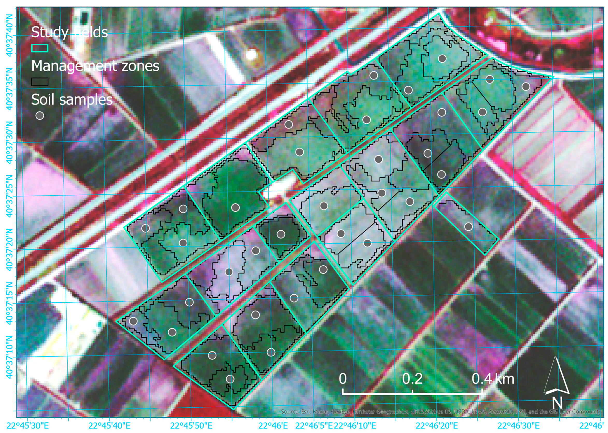
Thirty-five fields of 100 hectares total extent, around the town of Chalastra (40.6265N, 22.7307E, 6 m mean altitude) in the east part of the Plain of Thessaloniki, Greece were used for the study (
Figure 1). The mean extent of the fields was 2.82 ha, with 0.58 minimum and 4.46 maximum. The fields were under rotation with maize or cotton systematically after 2008.
Available historic yield data are recorded since 1998. These data, together with the farmer’s experience, indicate:
Significant yield variation between the rice fields (coefficient of variation 5.6% on average; larger than 10% for years 2009, 2010, and 2015);
An overall steady diminishing trend of rice yield by about 6% with temporary ups and downs over the years (coefficient of variation 12.4% on average; maximum at 19.5%).
These figures were taken as undisputed signs of spatiotemporal instability in rice growth between the fields of the farm and imposed problematic soil fertility potential. Farmer’s knowledge can be a reliable source of information about crop variation in different ways; for example, an indication by the farmer of the high, medium, and low yield zones, or clusters of different soil characteristics [
26,
27].
Below are the most important dates regarding the fertilization of the studied fields for the cultivation season of 2016:
Leveling: second half of April;
Seeding: 5–7 May;
Development fertilization: 11–14 May;
Tillering fertilization: 14–15 June;
Booting fertilization: 11–12 July;
Panicle heading fertilization: 9–10 August;
Harvesting: mid-October.
Other farming practices, such as weeding or pest management, are irrelevant to the subject, and thus, are not reported here.
2.2. Image Data
Three RapidEye images were acquired on 30 May 2015, 04 July 2015, and 26 August 2015, corresponding to critical growth stages of rice cultivation in the studied fields, i.e., before tillering, close to booting and after panicle heading, respectively. RapidEye constitutes of a 5-satellite constellation at 630 km in sun-synchronous orbit, each carrying an identical multispectral push broom imager. RapidEye was the first commercial imagery to supply an individual band in the red edge wavelengths, which is linked to critical crop parameters, such as chlorophyll content, biomass, and water content [
28]. The spectral bands of the RapidEye imagers are specified as follows:
B1: Blue (B): 440–510 nm
B2: Green (G): 520–590 nm
B3: Red (R): 630–685 nm
B4: Red Edge (RE): 690–730 nm
B5: Near Infrared (NIR): 760–850 nm
The RapidEye image dataset in hands was a radiometrically corrected and orthorectified product (3A-level), in the WGS84 projection system, UTM zone 34 north, with a 5-m pixel size. The images were composited into a new 15-band image (5 bands × 3 dates), which then underwent principal component analysis (PCA), thus allowing information concentration into a single band. The latter made a comparison of spectral and soil variations in the spatial domain, possible.
Before proceeding with data exploration and analysis, the pixels falling in an internal 15-m buffer from the fields’ boundaries were masked out, to neutralize the border effect. This effect is due to: (a) Existence of mixed pixels, i.e., pixels covering features not belonging exclusively to the cultivated part of the fields; and/or (b) misapplication of farming practices at the perimeter of the fields, which is quite common in most open-field cultivations.
2.3. Image Analysis
A methodology appropriate for detecting local variance in imagery is image segmentation, which is defined as the process of image division into spatially continuous, disjoint, and homogeneous regions, called image objects [
29]. In this study, the produced objects corresponded to the proposed management zones.
The Fractal Net Evolution Approach (FNEA) algorithm (also known as Multiresolution Segmentation), is one of the most common segmentation algorithms. With FNEA, image objects are created by grouping single pixels through a stepwise region-growing procedure of minimizing internal heterogeneity of each object until a pre-defined threshold (called ‘scale factor’) is reached [
30]. Scale factor influences the desired object size and shape [
31], according to one spectral and two shape criteria (namely, compactness and smoothness) [
32].
Indication of the optimum scale factor for a project is a difficult task, related to the specific objectives and availability of image data. Indicatively, Cánovas-García and Alonso-Sarría (2015) [
33] applied multiresolution segmentation on a high-resolution image of a large and heterogeneous agricultural area to optimize scale factor. Assessment of within- and between-zone variation was based on statistical metrics. Dragut et al. (2010) [
34] invented a software program (ESP) for evaluating the scale factor using local variance (LV) of object heterogeneity of the scene as a critical metric. Laliberte and Rango (2009) [
35] evaluated known texture measures for their correlation to different segmentation scales in mapping rangeland vegetation with 5-cm pixel true-color aerial photography. Manakos et al. (2016) [
36] investigated the optimum scale parameter for delineating ecological habitat types using a large set of textural features extracted from WorldView2 satellite imagery.
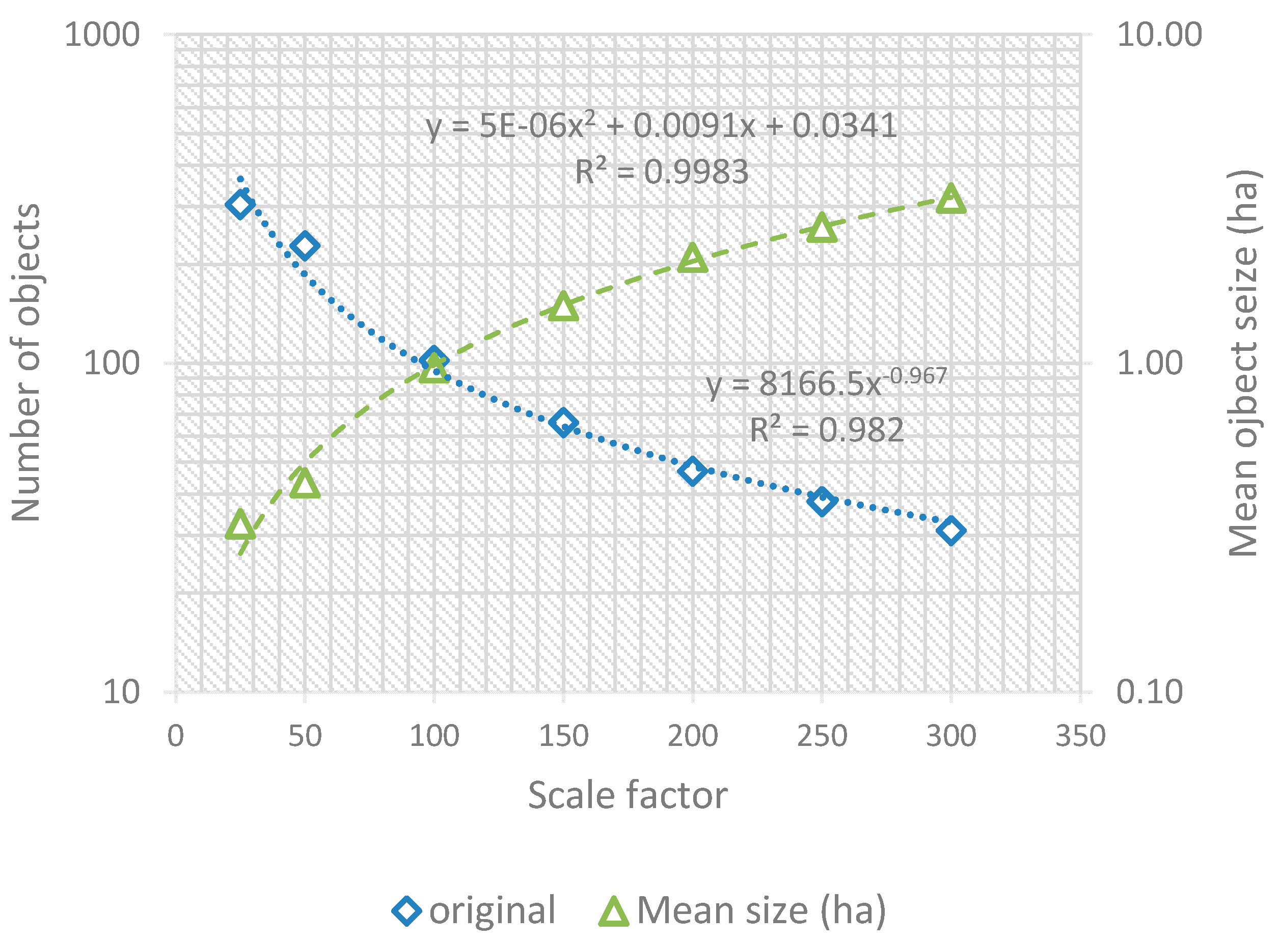
A sequence of segmentation levels was produced with FNEA, for the following experimental scale factors: 25, 50, 100, 150, 200, 250, and 300. The number of objects produced per scale factor (either before or after noise filtering) was found to follow a decreasing power-based line (
Figure 2); this type of equation between scale factor and number of objects has been proved to be typical with image segmentation of RapidEye images, as well as with other image types [
37,
38].
Optimal scale factors were indicated as those where within-zone variation is minimized, while between-zone variation is maximized; thus, where the difference between the two variations is maximized. The coefficient of variation was used as a measure of spectral variation derived from the first principal component (PC1) of the image. This approach is stemming from the ideas of Woodcock and Strahler (1987) [
39] about the local variance of image datasets in pixel-based analysis, adapted here to geographic object-based image analysis (GEOBIA).
2.4. Soil Mapping
A survey for site-specific soil sampling was conducted in late April 2016 before seedbed preparation. Using a GPS device, the soil was sampled at the centroids of the delineated management zones (a kind of cluster sampling). Cylindrical soil columns 30 cm deep were extracted and were sent for the full analysis to the certified soil laboratory of the Soil and Water Resource Institute, Hellenic Agricultural Organization DEMETER.
Autocorrelation tests of all physical and chemical soil properties at the sampled locations indicated that the soils of the farm were highly clustered in all cases (Moran’s I test; z-score values were ranging from 2.67 to 42.7). This fact implies that denser soil sampling would not provide significantly more critical information on the spatial distribution of soil properties in the specific farm.
Ordinary Kriging (OK) was applied as an interpolation method to produce continuous surfaces of soil properties from the point samples. Kriging has proved to produce realistic spatial patterns, while achieving high accuracies in soil mapping at various scales [
40]. Moreover, the evidence of strong spatial autocorrelation in the point dataset was in favor of using Kriging, instead of any other interpolator [
41]. According to Pozdnyakova and Zhang (1999) [
42], Kriging constitutes an appropriate method to study the spatial distribution of soil properties.
Furthermore, Ordinary Kriging was preferred over Universal Kriging, as the former is considered superior when anisotropy or strong trends are missing from the data, as it was depicted in the semivariograms of all the examined variables. A spherical model was followed with 12 neighboring points. Seventeen soil maps were produced from the samples, one per soil property.
Finally, each of the Kriging soil surfaces was upscaled into a zone-mean spatial layer, showing a single value (the mean) per zone. They were also upscaled to an entire farm-mean layer, showing a single value (the mean) for the entire farm. The rate of change for every cell between the entire farm-mean and the zone-mean layers (a downscaling process), as well as the rate of change of the original Kriging surfaces and the zone-mean layers (an upscaling process) were calculated, using the following formula (and for each soil property):
where
is the rate of change of cell
i values (in %),
is the value of cell
i in the original Kriging soil surface,
is the value of cell
i in the rescaled layer.
The outputs of Equation (1) indicate how more or less precise will be the zone-specific applications (resulting in either from the downscaling or the upscaling process) compared to the uniform or to the ideal, fully site-specific applications, respectively. In the former case (downscaling), within-zone soil variation is expected to be reduced (compared to the variation in the entire farm), whereas, in the latter case, within-zone soil variation is expected to be increased (compared to a cell-by-cell variation).
2.5. Analysis Summary
Summarizing the analysis steps, first, the management zones were delineated with image segmentation of the multi-temporal RapidEye imagery. Then, an equal number of soil samples were extracted from the centroid of each zone, and soil surfaces were produced with interpolation (continuous surfaces). Both image and soil variations were computed within and between the management zones, using the coefficient of variation (CV%), a metric allowing comparisons between different types of data (here spectral and soil data).
Finally, the soil surfaces were averaged per zone (zonal surfaces) and for the entire farm (uniform surfaces). The rate of change of every cell value of the zonal surfaces if replacing the uniform surfaces was recorded as a reduction of soil variation because of zoning (a downscaling process); whereas, the rate of change of every cell value of the zonal surfaces if replacing the continuous surfaces was recorded as an increase of soil variation because of zoning (an upscaling process). The overall approach can be considered as a multi-scale variation assessment framework (
Figure 3).
ArcGIS Pro © was used for organizing the geodatabase, for elementary image analysis (image compositing, Principal Component Analysis, etc.), interpolation, and geostatistics; eCognition Developer © was used for image segmentation; excel spreadsheets were used for descriptive statistical analyses.
3. Results and Discussion
3.1. Spectral Signature
The CV% of the 15-band RapidEye image composite in the whole farm was 46.4% on average (for all bands and all dates), with variation values ranging from 29.2% to 56.3% between image bands. Band-3 (red wavelength) on 4 July showed the biggest variation value (79.2%). The image of 26-August had the lowest CV% in all bands compared to the other dates (
Table 1).
The spectral signatures of rice crop within the studied farm (in terms of averaged spectral values per band) were only slightly different between the recorded dates; they differed mainly for B5 (near-infrared) for the signature of 30-May (
Figure 4).
3.2. Management Zones
The use of the coefficient of variation indicated scale factor 25 as optimum, while scale factors 50 and 150 were very close to optimum. However, scale 25 was excluded as containing a large proportion of noisy objects (i.e., objects-slivers at the edge of the fields); thus, only scale factors 50 and 150 remained as candidates for the optimum scale. As Karau and Keane (2007) [
43] argue, small scale factors are associated with “subtle changes resulting from management actions”, whereas only “large enough scale factors reflect the variation of ecological processes”. Small scale factors in this study were determined as those producing objects smaller than 1000 m
2, a threshold defined empirically with the farmer’s consultation [
44].
Scale factors 200 and beyond were far from optimum, as within-zone variation is increasing steadily, while between-zone variation is dropping at the same time. Existence of multiple optimum scales is not surprising as it is known that more than one critical parameter influences agricultural environment [
45]. Karydas et al. (2009) [
46] are in favor of the necessity to assess heterogeneity at multiple spatial scales in agricultural environments. At scale factor 300, the mean object size (after noise-filtering) was found to be larger than the mean field size, therefore the application of within-field management would not be possible; therefore, scale factor 300 was the maximum one tried.
In such complex environments, [
27] Oliver et al. (2013) argue that local variance alone is not enough to indicate optimum scale in multiresolution segmentation and that a second metric was required. As they suggest, the optimum scale should be defined in the view of a combination of two metrics, specifically where local variation is quite low and –at the same time- the 1st derivative of local variance vs. scale is maximized (
Figure 5). Similar conclusions were drawn by [
35,
47,
48] Laliberte and Rango (2009), Clausi (2002), and Barber and LeDrew (1991), who observed that contrast and dissimilarity were those texture features with the highest correlation (increasing and decreasing, respectively) with all segmentation scales.
According to the above, the scale factor where within-zone variation is minimized (1.19%) and at the same time the first derivative of within-zone variation reaches the maximum value (42.9%), corresponds to scale factor 150 (
Figure 5). At this scale factor, the number of produced zones was 66. This number corresponds to one soil sample per 1.5 ha (or 0.66 samples per ha); according to [
7] Wetterlind et al. (2008), a conventional grid density for cereals correspond to 1 sample per 2 ha (or 0.5 samples per ha). The between-zone variation in the PC1 image was calculated (also, as CV%) to 35.3% (from 46.4% of the global variation), whereas, the within-zone spectral variation was 2.2% on average, ranging between 1.2% and 5.5%, with almost half of the zones having values lower than 2%. These figures are indicative of the effect of zoning on the spectral data. In four cases (out of 66), the zones originally derived from the segmentation of the RapidEye composite were split manually further taking advantage of an image acquired with an Unmanned Aerial System (UAS) in the 2016 period for different purposes (crop monitoring) (
Figure 6).
3.3. Soil Surfaces
The results of the laboratorial analyses indicate that the soils were generally within normal physicochemical standards for rice cultivation. The farm soils belong to the Silty Loam, Loam, Clay Loam, and Silty Clay Loam types, which guarantee undisturbed rice cultivation, as they can retain moisture and heat (
Figure 7). Also, findings of electrical conductivity in the farm soils show to be quite far away from risky thresholds (3.5 mS/cm), in accordance with findings of [
24] Litskas et al. (2014) for the entire Thessaloniki Plain.
The organic matter in the farm was found, on average, slightly higher than the critical threshold of 2%. This can be attributed to the fact that during the last five years, the farmer has been practicing crop residue incorporation in the soil with tillage [
44]. Among physical properties, only soil acidity exceeded slightly the suggested upper threshold (7.5), a fact that has to be taken into account in the farmer’s fertilization strategy.
The variation of the properties measured in soil samples ranged within a wide interval (from 1.8% for soil acidity up to 160% for phosphorus), while their overall variation was 33.7% (
Table 2). Wilding (1985) [
49] has classified heterogeneity degree of soil properties within a farm management system in three generic categories:
When exhibiting CV < 15%, soil can be considered as “least variable”.
When exhibiting 15% < CV < 35%, soil can be considered as “moderately variable”.
When exhibiting CV > 35%, soil can be considered as “most variable”.
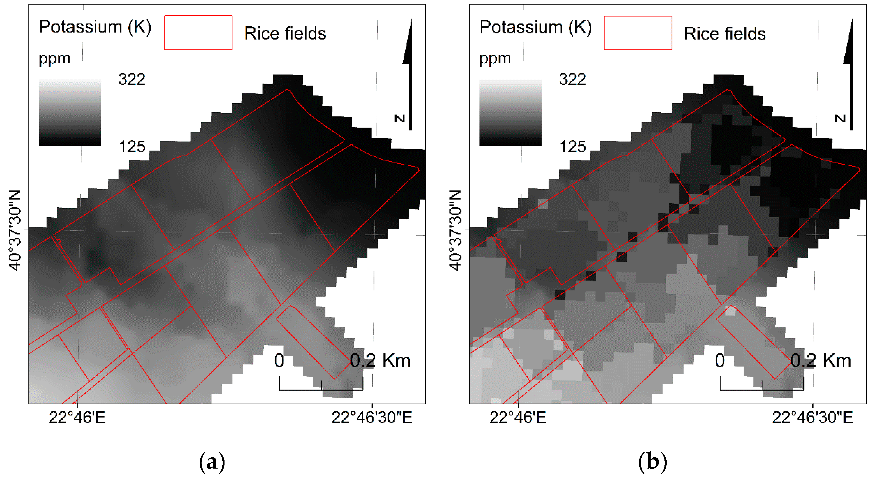
According to the above classification, it can be noted that six properties were found to be highly variant within the farm (sand content, electrical conductivity, nitrogen content, phosphorus content, available zinc content, and available boron content); another nine properties were moderately variant (silt content, clay content, organic matter content, total CaCO3 content, potassium content, alternative magnesium content, available iron content, available manganese content, and available copper content); and only two of the measured properties were at low variant levels (soil acidity and bulk density); calcium was not possible to be evaluated for variance as the records were provided in lumped form by the laboratory (as “>2000 ppm”). As the overall variation of soil properties based on the collected samples was 33.7%, the farm soil can be considered as moderate to high variable, according to Wilding (1985) [
49].
Application of Ordinary Kriging (OK) for each of the soil properties sampled (except Ca), resulted in 17 surfaces. Because the sample size was not big enough for independent validations of the Kriging surfaces, the mean standardized error (MSE) was used as an indicator of unbiased spatial predictions by means of data cross-validations. The resulting MSE values were very low, a fact showing that the surfaces derived from the applied Kriging models, were unbiased for all examined soil properties (
Table 3).
Furthermore, comparison of the means of the sample set and the interpolated surfaces (per soil property), revealed ignorable differences; in all cases, differences were lower than 3%, with only P, Mg, and N reaching differences around 11%, 6%, and 4%, respectively (
Figure 8).
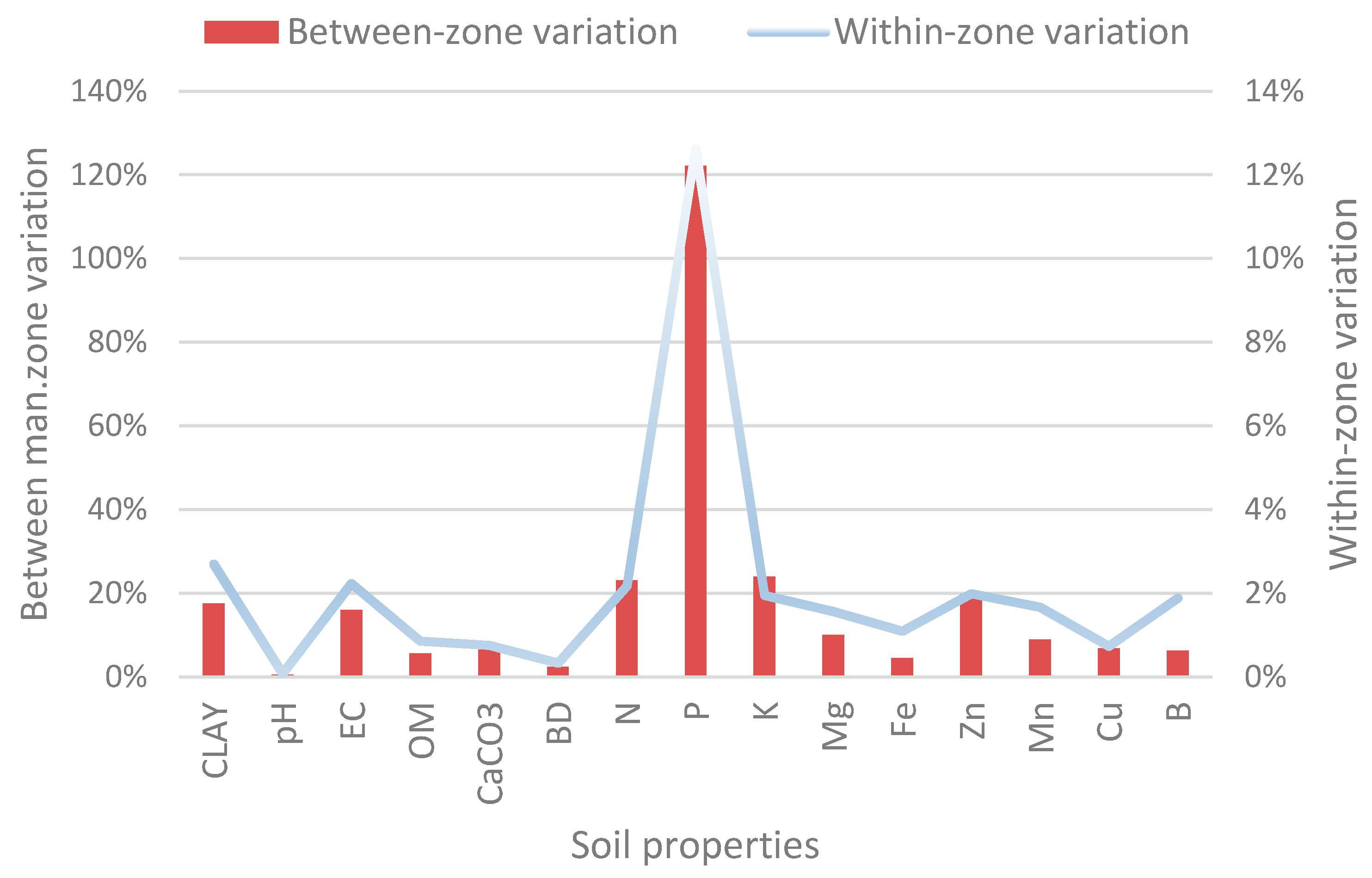
3.4. Assessment of between and within-Zone Variation
The between-zone variation of the soil surfaces was found to be 18.2% on average, a value characterizing the specific soils as “moderately variable” (i.e., >15%) [
49]; the maximum value was recorded for phosphorus (119.4%). It was significantly lower, however, than the variation recorded between the soil samples (33.7%). The within-zone soil variation ranged from 0.4% to 9.3% with an average of 4.5%, while for most nutrients it was very low; N, P, K, and Zn had 2.2, 11.2, 1.9, and 2.7, respectively, far smaller values from their corresponding between-zone variation values (25.7, 121.3, 21, 21.2, respectively) (
Figure 9).
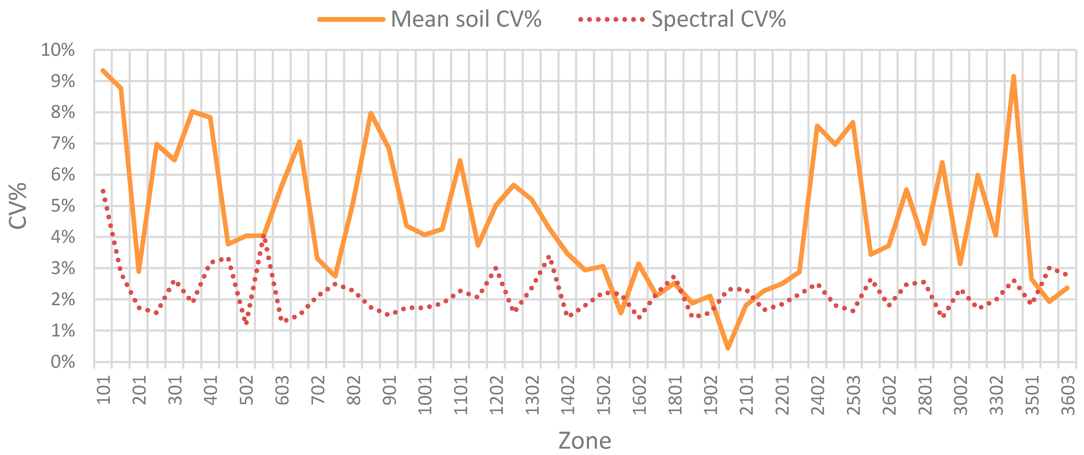
Spectral within-zone variation ranged from 1.2% to 5.5% with an average at 2.2%. The mean of the ratio of the two variations (soil/spectra) was 2.21 and the median 1.92. There was no evidence that a single soil property could explain alone the within-zone spectral variation captured by the imagery (
Figure 10).
3.5. Rescaling Effect Assessment
Upscaling the Kriging soil surfaces into zone-mean layers and to entire farm-mean layers resulted in a set of fifty-one new soil surfaces (3 scales × 17 soil properties) (
Figure 11).
Application of Equation (1) on the parameters of the downscaling process from the uniform single-valued layers to zonal layers, resulted in a mean variation reduction of 12.5%, with P being far the highest value (72%) and Clay content, EC, N, K, and Zn having values over 10%. The rest of the properties were all below 10%, with pH having the lowest value (0.37%). Mean variation increase (due to upscaling from the continuous layers to zonal layers) was 1.93 on average and reached 10.6% for P (far the highest value), while all the rest of the properties were found quite below 2.5%. As it can be conceived from these results, variation reduction was far higher than variation increase in all cases from three to ten times (about six times on average), with the mean difference between variation reduction from variation increase to be 10.6% (
Figure 12). Practically, this means that the zone-specific applications will be far more precise compared to the uniform ones and at the same time only little less precise compared to ideal, fully site-specific applications.
3.6. Fertility Potential
All the physicochemical soil properties analyzed were found to be within normal value ranges. Specifically, soil texture was shared between SL, L, CL, or SCL types; soil acidity was slightly above the upper threshold of 7.5, while electrical conductivity was far below the critical threshold of 3.5 mS/cm; the organic matter was slightly over the critical value of 2%; while bulk density was close to an expected value (1.41 g/cm3). Regarding nutrients, only nitrogen, phosphorus, potassium, and zinc had values out of normal range in extended parts of the farm, whereas, the rest of the nutrients were mostly within normal ranges. Electrical conductivity was far below from the well-established threshold of 3.5 mS/cm for the entire farm. However, if a stricter threshold (e.g., 1.3 mS/cm) were set, 44% of the farm’s soils would overpass it. It must be noted that electrical conductivity is a commonly used factor of judgment for underlying soil variation [
50].
Using thresholds from the literature [
51], every soil surface was divided into three zones: One for below the low threshold, one for between the low and the high threshold, and one for above the high threshold. Especially for nutrients, these zones can be called deficiency, adequacy, and excess zones, respectively (
Table 4). In many cases, the excess might be equally harmful with deficiency, as for example, for phosphorus (
Figure 13).
According to the deficiency, adequacy, and excess maps, it was found that nitrogen was in serious deficiency throughout the farm, with alternative magnesium and calcium in excess everywhere. Phosphorus and potassium were partially in deficiency, in adequacy, or excess; potassium was in deficiency or excess only in very limited extents. In total, 85% of the farm was within favorable nutrient ranges.
As for the micro-nutrients, iron and copper were in excess throughout the entire farm, whereas zinc was in moderate deficiency (0.74 ppm) in 87% of the farm soils. According to IRRI (2017) [
51], zinc is critical in chlorophyll production and membrane integrity. Boron was in deficiency only in a small extent (12%), though very close to the critical threshold, whereas manganese was adequate almost everywhere, slightly over the acceptable value.
Finally, phosphorus and zinc were in deficiency together throughout about in 40% of the farm extent. However, simultaneous deficiency of phosphorus and boron was detected only in 4% of the farmland.
3.7. Recommendations
The findings of the soil analyses indicated that fertility variation either between or within the studied fields was significant for rice cultivation. The satisfaction of these differentiated crop requirements was based on the application of distinct fertilizer amounts per zone. In practice, every zone was taken as a relatively homogeneous unit of application; thus, 66 recipes were prepared and applied at four critical growth stages (development on 11–14 May, tillering on 14–15 June, booting on 11–12 July, and panicle heading on 9–10 August). The fertilization recipes were computed considering the following sources of advice:
Fertilization was the only farming practice to follow a site-specific strategy, whereas the rest of the practices (seeding, irrigation, weed management, pest management, and harvesting) remained conventional for 2016 and mainly uniform throughout the farm. The specific amounts and chemical compositions of the fertilizers per zone were determined according to the minimum requirements per nutrient, as these were implied by the produced interpolated soil maps.
Indicatively, nitrogen applications ranged from 140 to 342 kg/ha, with a mean of 222 kg/ha and a coefficient of variation 12.6% (average weighted according to zones’ area); note that N variation reduction in soil by zoning was 15.09%. Regarding phosphorus, its applications ranged from 0 to 170 kg/ha, with a mean of 91 kg/ha and a coefficient of variation 58.6%; the explained P variation in soil was 72.14%. Also, potassium applications were quite differentiated, with a mean of 20 kg/ha, a range of 30 kg/ha and a coefficient of variation 42.5%; the explained K variation in soil was 17.48% (
Figure 14).
4. Conclusions
This research showed that image segmentation applied on a multi-temporal composite of RapidEye images acquired during critical growth stages of rice crop, was sufficient to delineate management zones for site-specific soil sampling. However, the application of the local variance method alone with the PC1 image of the composite, showed to have limitations in indicating the optimal number of management zones in advance of soil sampling. More sophisticated algorithms are necessary to indicate the optimum scale factor for segmentation, and thus, the optimal number of zones, in a more straightforward way; for example, Karydas (2020) [
38] has proposed use of fractal geometry in scale factor optimization for different types of imagery. Also, different types of imagery will be tested for zone delineation under a new, more automated process framework.
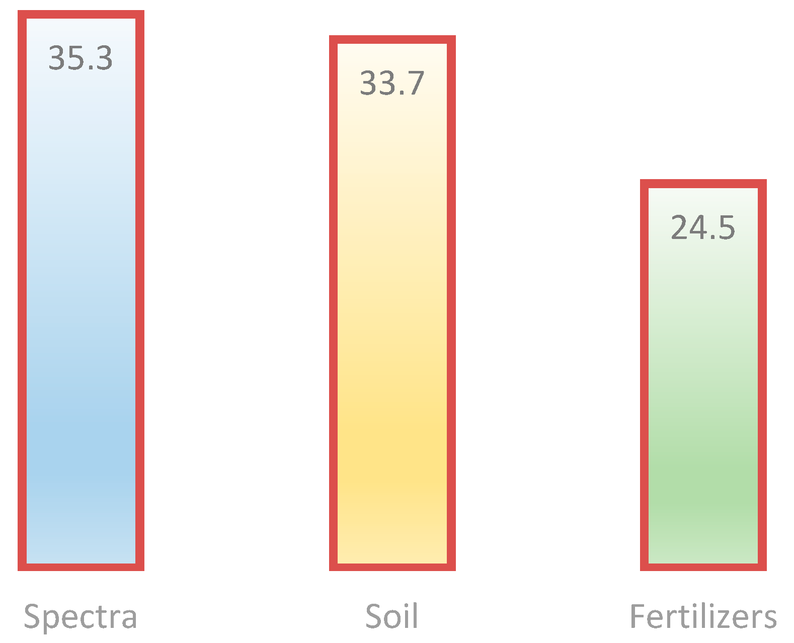
The results indicate that variation in imagery and soil in the studied rice fields were high and moderate, respectively. The between-zone spectral variation was found to be 35.3%, while between-zone soil variation was 33.7% on average; the mean within-zone variation was 18.2% for the soil properties (
Figure 15). These levels of variation show that zoning for site-specific soil sampling was captured reliably by the multi-temporal RapidEye imagery. Moreover, the detected soil variation was significant enough to dictate zonal fertilization recommendations, which variated by 24.5% for nitrogen, phosphorus, and potassium (i.e., the macro-nutrients usually included in input fertilizers). Finally, it was proved that zonal applications reduced soil variation, thus increasing precision in applications by 18.6%, compared to conventional uniform applications.


