SAR Sentinel 1 Imaging and Detection of Palaeo-Landscape Features in the Mediterranean Area


1
Italian National Research Council, C.da Santa Loja, Tito Scalo, 85050 Potenza, Italy
2
National Authority for Remote Sensing and Space Sciences, Cairo 1564, Egypt
3
DICEM (Dipartimento delle Culture Europee e del Mediterraneo), University of Basilicata, Via Nazario Sauro 85, 85100 Potenza, Italy
*
Author to whom correspondence should be addressed.
Remote Sens. 2020, 12(16), 2611; https://0-doi-org.brum.beds.ac.uk/10.3390/rs12162611
Submission received: 27 May 2020
/
Revised: 5 August 2020
/
Accepted: 11 August 2020
/
Published: 13 August 2020
(This article belongs to the Special Issue Remote Sensing, Spatial Analysis, and GIS for Natural and Cultural Heritage Documentation, Monitoring, and Preservation)
Abstract
:The use of satellite radar in landscape archaeology offers great potential for manifold applications, such as the detection of ancient landscape features and anthropogenic transformations. Compared to optical data, the use and interpretation of radar imaging for archaeological investigations is more complex, due to many reasons including that: (i) ancient landscape features and anthropogenic transformations provide subtle signals, which are (ii) often covered by noise; and, (iii) only detectable in specific soil characteristics, moisture content, vegetation phenomenology, and meteorological parameters. In this paper, we assessed the capability of SAR Sentinel 1 in the imaging and detection of palaeo-landscape features in the Mediterranean area of Tavoliere delle Puglie. For the purpose of our investigations, a significant test site (larger than 200 km2) was selected in the Foggia Province (South of Italy) as this area has been characterized for millennia by human frequentation starting from (at least) the Neolithic. The results from the Sentinel 1 (S-1) data were successfully compared with independent data sets, and the comparison clearly showed an excellent match between the S-1 based outputs and ancient anthropogenic transformations and landscape features.
1. Introduction
For most of the 20th century, aerial photography was the primary remote sensing tool adopted for landscape archaeology and for detecting buried archaeological structures through visual interpretation based on archaeological proxy indicators [1]. The most common archaeological proxy indicators are generally known as crop, soil, shadow, and damp marks and are caused by the presence of buried remains and traces of ancient environments still fossilized in the modern landscape. These features induce spatial anomalies (in vegetation growth and/or status, surface moisture content, and micro-reliefs) that are generally not visible in situ but only evident from above [2]. In recent decades, significant improvements were obtained in the identification of archaeological proxy indicators from very high resolution (VHR) satellite optical and synthetic aperture radar (SAR) data [3].
Starting from this heritage, new applications and developments are expected [4,5,6,7,8,9,10,11], particularly from the use of open data, such as satellite Sentinel 1 and 2 (S-1 and S-2) that are part of Europe’s ambitious Copernicus program [11]. All the Sentinel missions were released under an open data policy to foster knowledge, innovative applications, and advanced developments. In particular, S-1 data were used for the monitoring of cultural heritage (CH) [12], and recent pioneering studies have highlighted that S-1 can be useful to extract information regarding the contemporary and past landscape (the detection of buried or emerging archaeological remains), to infer changes in the current and former environment, and support the discovery of buried archaeological sites. In more detail, early investigations addressed the underwater palaeo-landscape (bathymetric assessment) of the North Sea [13], and land-based archaeological landscape in Egypt to discover potential buried archaeological sites in the agriculture environment [14].
Despite these very promising, early results, the use of S-1 for archaeology is still an open issue and presents current and future challenges. In this context, compared to optical data, the use and interpretation of radar data for archaeological investigations is much more complex for many reasons, in particular as archaeological investigations are focused on the detection of subtle signals (often covered by SAR noise), and only detectable in specific conditions [15]. For these reasons, over the years, SAR based archaeology has been historically limited by the low spatial resolution of the early sensors, even if important archaeological discoveries were made in vast deserted areas, as in the case of the Saharan radar-river [16].
Even if the use of satellite radar in archaeology is still today in its experimental stage, it undoubtedly offers great potential for manifold applications, such as the reconstruction of the palaeo-landscape [16], the detection of buried sites [17], along with the documentation and monitoring of cultural heritage as performed in recent studies conducted using very high-resolution satellite radar data such as TerraSAR-X and COSMO-SkyMed [18,19]. SAR based archaeology poses pressing critical issues, linked with the lack of investigations, particularly those conducted in diverse environments (desert, semiarid, Mediterranean, etc.), different land use/cover types, along with the needs to improve the interpretation and modeling approaches, which may be adjusted or developed ad hoc for different environments.
This study provides a contribution in this context, focusing on the use of S-1 data in the Mediterranean environment to detected ancient landscape features and anthropogenic transformations. To this aim, a significant test area (larger than 200 km2) was selected in the Foggia Province (South of Italy), as this region is characterized by long human frequentation (from the Neolithic time until now) and, consequently, for millennia has been continuously involved in and affected by anthropogenic human transformations. Across and around the study area, large Neolithic villages, pre-Roman routes, and Roman villas have been discovered during the last century.
2. Materials and Methods
2.1. Study Area
The area of interest, known as Tavoliere delle Puglie, lies between the city of Foggia and Lucera in the Apulia Region (Figure 1a). The study area is situated within geographical coordinates between longitude 15°20′30′′ and 15°37′ E, and latitude 41°28′30′′ and 41°35′ N, and covered approximately 224 km2 (Figure 1b). The Apulian palaeo-environment coast has been reconstructed by the multilayers of sediment cores drilled in various coastal areas and characterized by different landscapes, in addition to its various ancient civilization sites (e.g., Neolithic, Greek/Roman, and medieval settlements) [20].
From the geological point of view, the investigated area belongs to the central part of the domain of the Apennine foredeep. The deposits formed during several middle and late Quaternary depositional phases were strictly linked with the interplay between the regional uplift and sea-level fluctuations. The oldest terrains, cropping out mainly in the western area, are represented by the argille subappennine unit that form the hills of Lucera (very close to the study area) and consists of a poorly bedded alternation of clays and silty clays of marine origin, lower Pleistocene in age. All the deposits of this unit can be referred to several systems of alluvial fans in seven systems. Terraced deposits are located at different elevations on present-day river beds. Our study area is included in a system, dated to the Upper Pleistocene, named Motta del Lupo, which derives its toponymal from the site of Motta de Lupo, archaeologically known for a Neolithic settlement. The Motta del Lupo system consists of alluvial terraces composed of brow fine sands interbedded with thin layers of pelites. This unit lays in erosive unconformity on the argille subappennine unit and/or on the deposits of older systems. The observed thickness varies from a few meters up to a maximum of 10 m [21].
The Tavoliere is characterized by multi-layered settlements generally referable to Neolithic, Roman, and medieval ages, which make it one of the most important archaeological areas in Southern Italy [22]. The first ancient phase of human settlement is the Neolithic, herein dated between 6500 and 6200 BC (e.g., Puglia region) [23,24], or earlier [25,26]. The Tavoliere includes the area of interest of this study, which remained unknown until the 1940s, when John Bradford recognized Neolithic features from the vegetation marks visible from the RAF and USAAF aerial photographs [27]. Up to 2014, approximately 570 georeferenced sites were found in the areas covered by the original RAF and USAAF air surveys (less than 50% of the total area of the plain), to which we can add 206 known sites that fall outside these mapped areas [28]. Large Neolithic villages, pre-Roman routes, and Roman villas have been discovered during the last century across and around the study area located on the Northeast of Lucera and on the Northwest of Foggia.
The landscape is characterized by the presence of several palaeorivers and palaeochannels, and this is of interest considering that, in the Mediterranean Basin regions, river management generally [29] started in the Neolithic societies during the humid phase of the Holocene, characterized by a humid and rainy climate from approximately 7500 to 4000 BC [21,22,23,24,25,26,27,28,29,30].
Land management in the early stages of Neolithic sedentary agriculture and its impact on the landscape and the organization of settlements is an open issue for archaeologists. In particular, the Neolithic culture of Puglia and southern Italy was one of the first that developed in Europe. The Neolithic culture in Apulia was complex, with settlements built according to their functions: (i) mountain or sub-mountain settlements for pasture (e.g., Murgia area); (ii) near the extraction points and caves (e.g., the coast to the north-east of Foggia); and (iii) in the Tavoliere, along the rivers, for agriculture [31,32,33,34,35,36].
The practice of agriculture at the end of the glaciation period is well documented in the area by archaeologists and archeobotanists and was closely linked to the use of hydrological resources [37,38] (Figure 2). In particular, in [36,39] (Figure 2), the relationship between settlements and rivers is well represented.
Therefore, the detection of palaeo-hydrography is fundamental for the study of the first human settlements, where our knowledge starting from the Neolithic, or earlier, depends on the understanding of the local river dynamics and hydrological variability [29].
2.2. Rationale, Data Set, and Processing
The recognition of archaeological and palaeo-environmental proxy indicators from radar imaging is more complex compared to optical indicators due to a greater number of parameters that characterize SAR data, including (i) surface roughness; (ii) moisture content, linked to dielectrical properties of the target; (iii) the radar system in terms of the operating frequency, polarization, angles, and viewing geometry (ascending or descending); (iv) the characteristics of the sensed surface in terms of the land use and cover types, topography, and relief; along with (v) the morphological characteristics. It is crucial to consider that these features are generally not permanent signals but only “visible” in specific observation conditions depending mainly on the crop phenology, soil type, and moisture content, and in turn, the weather conditions. Therefore, in order to assess the potentiality of Sentinel-1 in the detection of ancient anthropogenic transformations and palaeo-hydrography, a time series for 2014–2019 of Sentinel-1 GRD (IW) was used for the study area to capture both the inter- and intra-year variability expected in the “visibility” of the archaeological proxy indicators. Considering that SAR data are influenced by the radar system itself, in terms of angles, viewing geometry (ascending or descending), and polarization, the data set was selected including both:
- ✓
- ascending and descending modes and;
- ✓
- VV and VH polarizations.
The inter- and intra-year analysis of the data collection, downloaded for free from the ESA [41] and Alaska Satellite Facility (ASF) data [42] websites (Table 1), enabled us to identify, for some representative known archaeological buried remains, both the best period of the year and the best SAR based parameters to capture the archaeological proxy indicators (Figure 3).
Radar S-1A and B satellite images were downloaded from the Sentinel Scientific Data Hub and Alaska Satellite Facility (ASF) data. The pre-processing and processing were done using SNAP 6.0 (Italian National Research Council, Tito Scalo, Potenza, Italy) coupled with tools available in ArcMap 10.4.1 (National Authority for Remote Sensing and Space Sciences, Cairo, Egypt) and ENVI 5.1 software (National Authority for Remote Sensing and Space Sciences, Cairo 1564, Egypt).
2.3. Data Processing
In the current study, we tested the Sentinel-1 GRD (IW) acquisition mode’s observations for measuring its suitability in detecting the buried settlements in the study area. In more detail, we used the Apply Orbit File, Thermal Noise Removal, Calibration, Speckle filtering, Range-Doppler Terrain Correction, Conversion to dB, and Filtered band tools to analyze the Sentinel 1 data. Both VV and VH polarizations investigated. The polarisation of SAR imagery is commonly denoted by two letters, the first is the transmitted, and the second is the received [43]. In this study, the VV (vertical transmission; vertical reception) and VH (vertical transmission; horizontal reception) amplitudes were used and projected to ground range using an Earth ellipsoid model, WGS84. The acquired radar data for the study were from Sentinel 1A/B (C-band) interferometric wide (IW) swath mode with the mode products at SAR Level-1 Ground Range, Multi-look, detected (GRD) on 15 October 2014, 21 October 2015, 28 October 2016, 17 October 2017, 17 October 2018, 19 October 2019, and 25 October 2019.
The data processing steps were: Apply Orbit File, Thermal Noise Removal, Calibration, Speckle Filtering, Range Doppler Terrain Correction, and Conversion to dB, along with the Filtered band as follows:
2.3.1. Apply Orbit File
Generally, orbit state vectors, contained within the metadata information of SAR products, are not accurate. The precise orbits of SAR satellites are determined after many days and became available after the generation of the final product by days-to-weeks. SNAP software tools allow the SAR data users to update the orbit state vectors for each scene in its product metadata, provide velocity information, and give an accurate position for the satellite according to the radar tool [44]. Sentinel-specific processing facilities also host the relevant Level-1 instrument processor components [45]. We considered the expected accuracy of “resituated orbits” sufficient for computing interferograms without artifacts [46].
2.3.2. Thermal Noise Removal
In addition to the speckle noise, SAR images suffer from additive thermal noise, especially when the backscattered power is low. Thermal noise removal was used to reduce the noise effects in the inter-sub-swath texture, in particular, to normalize the signal of the backscatter within the entire Sentinel-1 radar image and resulted in reduced discontinuities between sub-swaths for every scene in the multi-swath acquisition modes. The ESA provided thermal noise information for each image in XML formatted files [47]. For removing the thermal noise for the level-1 product, the SNAP provided operator for Sentinel-1 radar data was used to re-introduce the noise signal and allow for re-application of the correction [48].
2.3.3. Calibration
This step includes two main tools; radiometric correction and the multilooking technique. Radiometric correction of an image was conducted so that the pixel values truly represent the backscattering of the reflecting surface. After data pre-processing, the calibrated data were filtered to reduce the inherent SAR speckle noise and clipped in range and azimuth to remove the image border noise. The result of the pre-processing is a re-projected, radiometrically calibrated, and rescaled normalized radar cross-section (NRCS) image [49]. For a particular azimuth time, the thermal noise was estimated in the slant range coordinates by calculating the range spreading loss vector and the elevation beam pattern vector, and applying the scalar contributing factors. According to the Sentinel-1 GRD products, in subtracting the noise from the power-detected image, the thermal noise vectors were converted to ground range coordinates and applied to the data. When calibrating the product to σ, γ, the noise vector must be scaled by the corresponding calibration look-up table (LUT) (, γ, or , respectively) as in Equations (1)–(4) [49]:
where depending on the LUT selected to calibrate the image data:
After obtaining the calibrated noise profile, removing the noise from the GRD data became available by subtraction. During the TOPSAR sub-swath merging, the noise vectors for any pixel ί that fell between points in the LUT value were also merged into one vector by merging two adjacent ground range images [50].
The calibrated noise profile can be applied to remove the noise by subtraction. Application of the radiometric calibration LUT and the calibrated de-noise LUT can be applied in one step as in Equation (5) [51]:
After the radiometric calibration, the spatial resolution is degraded but the image noise is reduced and approximate square pixel spacing is achieved. Therefore, the Multilooking technique as a tool in the SNAP software is required to reduce the speckle noise effect, reaching a spatial resolution of 20 m [52].
2.3.4. Speckle Filter
Speckle filtering is needed to suppress the noise and to remove observations that are not affected by noise and contain valuable land surface information. To remove the speckle, the refined Lee filter was applied as it maintains the detail of the standing boundary [53].
2.3.5. Range-Doppler Terrain Correction
Geometric correction using the “Range-Doppler Terrain Correction (RDTC)” tool in the SNAP software was used for converting the Sentinel-1 GRD data from ground-range geometry into a map coordinate system [54]. In more detail, terrain correction was applied to transfer the single 2D of raster radar geometry to accurately geocode the images by correcting SAR geometric distortions using digital elevation model (DEM) from the Shuttle Radar Topography Mission (SRTM) (that allowed us to consider the local elevation variations) for geocoding Sentinel 1 imagery [55]. Step one was choosing the imported SAR data as an input in orthorectification and the directory output to save the orthorectified image. Both the input and output data were saved in one projected file. The second step will define the parameters and bands amplitude VV and VH that will be processed using Shuttle Radar Topography Mission (SRTM 3 Sec) as inputs to the digital elevation model (DEM) data. This was automatically downloaded, as both of DEM and Image Resampling use the bilinear interpolation method. We defined pixel spacing to 30 m, the corrected image was resampled to 30 m from 10 m, and thus this new size fitted both the used map projection, the orthorectified SAR data size in the GLS-2000, UTM, and also the datum, WGS 1984. The areas without elevation were masked based on DEM data. Then, the process was running automatically after defining the parameters [54].
2.3.6. Conversion to dB
This step was applied to change the “Sigma0_VH_db” and “Sigma0_VV_db” bands from the virtual bands to files. In this conversion, the unitless backscatter coefficient was converted to dB using a logarithmic transformation [52].
2.3.7. Filtered Band
Filtration tools are included in SNAP software that can be used in the processing steps for the improvement of the analyzed data. These include detect lines (e.g., horizontal edges, vertical edges, compass edge detector, etc.), detect gradient (e.g., emboss), smooth and blur, sharpen, enhance discontinuities, and nonlinear filters. There are also morphological filter tools (e.g., erosion, dilation, opening, and closing) that can be used in the morphological field.
2.3.8. Time Series Analysis for Extracting the Backscatter Values
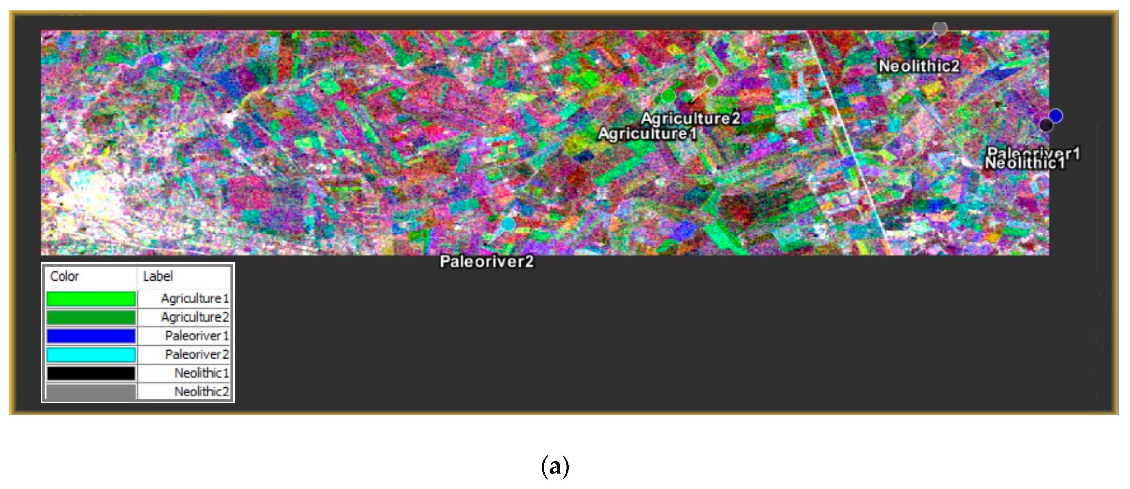
The SAR data were chosen to make the comparison between the backscatter values for three classes; Neolithic, palaeo-hydrography (palaeoriver and palaeochannel), and agriculture (non-archaeological sites). The data were clipped for all the dates of October in 2014, 2015, 2016, 2017, 2018, and 2019 to test the best dates for obtaining the potential archaeological and palaeo-hydrographic features according to the backscatter values of the chosen points. The time series analysis was tested for ten months in 2019 to cover the four seasons in March, April, May, June, July, August, September, October, November, and December. One batch was built to apply on all tested data with calibrate, terrain correction, speckle filter, and liner to dB. Two samples were measured for every class, and the median was calculated cross the VV and VH polarizations for both pass directions (ascending and descending) according to Equation (6):
where is the image pixel, is the vector that formed by the band values of the image, the , is a vector composed of the mean value of the background pixels in each image band, and is the covariance matrix of the image bands (that computed cross the background pixels) [56,57].
2.3.9. Computation of Polarimetric Indicators
The ratio of σ° VV/VH, which is the ratio between σ° VH and σ° VV.
3. Results
In this section, we will discuss the results obtained from the analysis of the whole time series of 2014–2019 made to characterize the (i) intra- and inter-year variability in the visibility of palaeo-hydrographic features and archaeological proxy indicators (as explained in Section 2.2).
In order to make the interpretation of S-1 data easier, the SAR data set related to 2019 were compared with the 2019 multi-date S-2-data set elaborated as detailed in [58] (Figure 4).
It is important to consider that the whole area under investigation is classified as arable land in the Corine land cover [59] and devoted to agricultural activities, mainly cereal crops. So that, in the study area, the October month is a period before snow, and therefore, expected to be mainly characterized by the presence of bare soil and spontaneous herbaceous cover (see Figure 4b) as evident from the S-2 RGB false color where the green areas are related to vegetation (mainly herbaceous cover) whereas the brown areas are mainly related to bare soil. These surface conditions can be considered ideal for the detection of soil moisture anomalies linked to archaeological proxy indicators, such as soil and damp marks. For SAR sensors operating at the C band as S-1, we have to consider the interfering effects that are introduced by surface roughness.
Sentinel-1 for the Identification of Archaeological Proxy Indicators and Palaeo-Landescape Elements
SAR analysis conducted in the study area using Sentinel-1 data allowed us to assess the potential of this tool, thanks to the integration of data obtained with multispectral/multitemporal images obtained from Sentinel-2 [58] and ancillary data from bibliography and other sources.
SAR radar backscatter measurements were influenced by both the terrain structure and surface roughness, and it is expected that the more roughness, the greater the backscatter (resulting in a bright feature). The diverse polarizations, in our case, VV and VH helped in discriminating and estimating the different contributions due to (i) the moisture content and (ii) roughness.
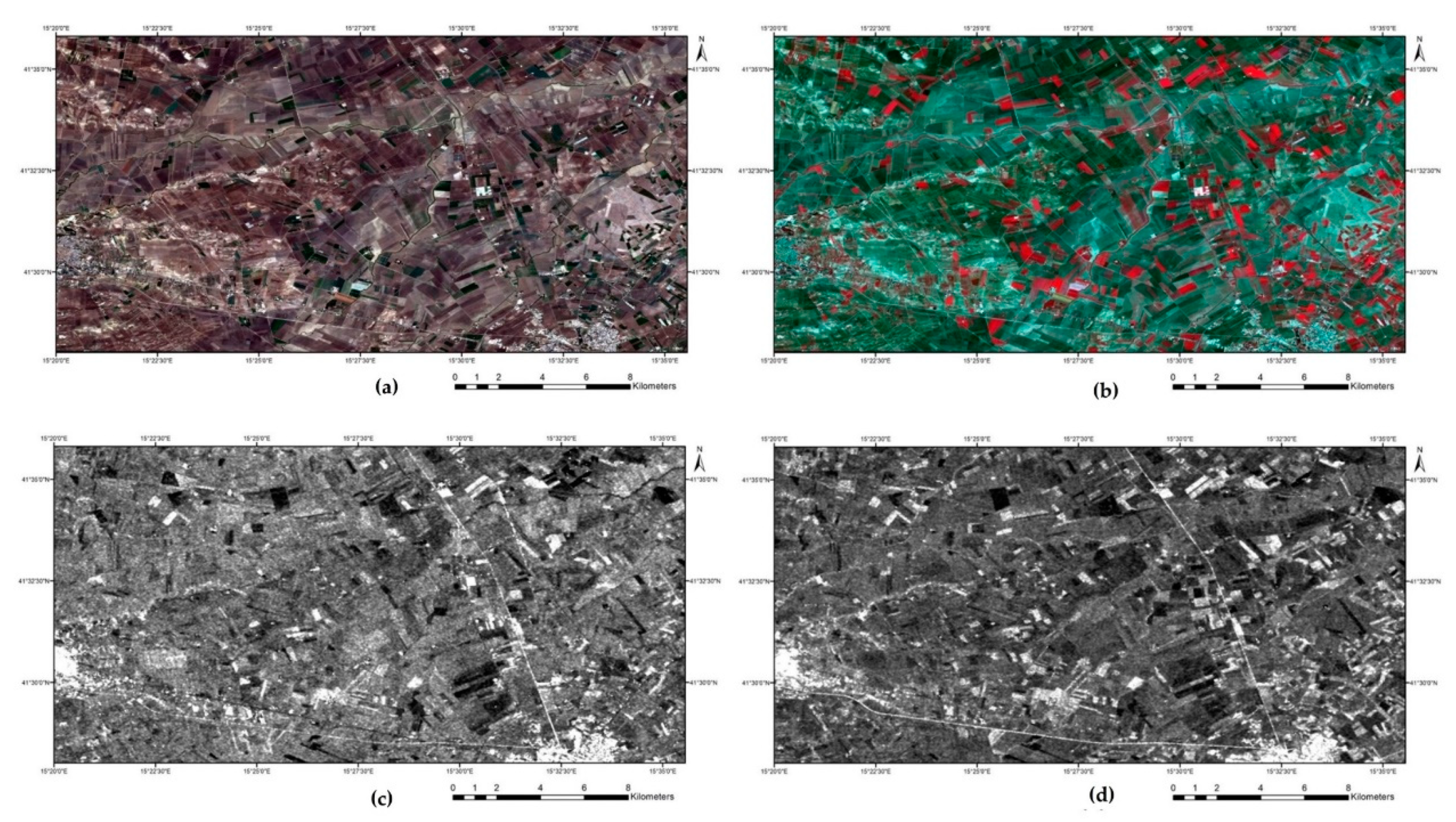
In the final analyzed S-1-A and B images (October 2014, 2015, 2016, 2017, 2018, and 2019), some black ditches and white complex areas were identified with archaeological potential for buried archaeological remains in the study area (Figure 5a–f).
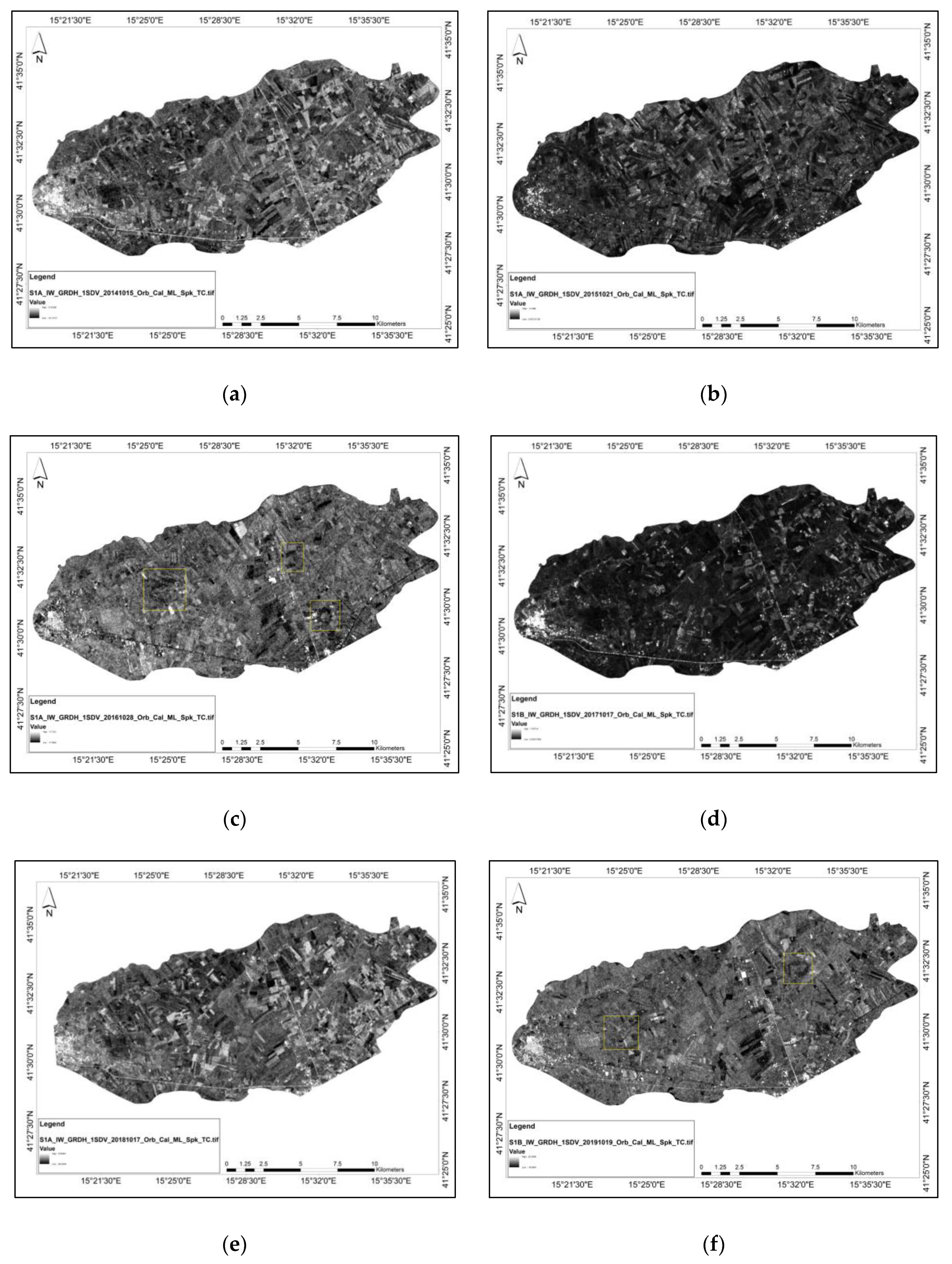
We compared the SAR based anomalies of potential archaeological interest with the results from (i) previous investigations and ancillary data as the aerial photographs acquired by RAF and USAAF air surveys photographs and (ii) published researches [60,61,62,63]. The results from these comparisons, along with the analyses of the shapes and size of the discovered archaeological features suggested that they were related to the Neolithic period. Due to the noise present in the Sentinel-1 data, the first activity was to identify known archaeological complexes so as to understand the type of result provided by the S-1 SAR sensor (Figure 5). The features in the S-1 analyzed images (Figure 5c,f) had the typical shape of the Neolithic settlements of the Tavoliere as circular with concentric ditches that enclosed smaller ditches and huts [36] (Figure 6).
These detected shapes are supposed to date back to the Neolithic Era according to the findings of previous works [30,62,63,64]. The analysis allowed us to identify SAR data sites already known in the bibliography, such as those east of Lucera as: (i) Masseria Sarcone and (ii) Masseria Villano (Figure 7). Within the S-1 SAR data, the outer ditches of the settlements and the smaller inner ditches are visible, according to Neolithic settlement shape (Figure 6).
The results obtained from the diverse acquisitions of S-1 showed how the visibility of features of archaeological interest and other elements useful for the reconstruction of the ancient landscape are influenced by factors, such as: (i) the weather; (ii) soil moisture; (iii) temperature; and (iv) soil roughness (see Discussion). In the present study, the images that gave the best results were the ones produced by the acquisition of 19 October 2019.
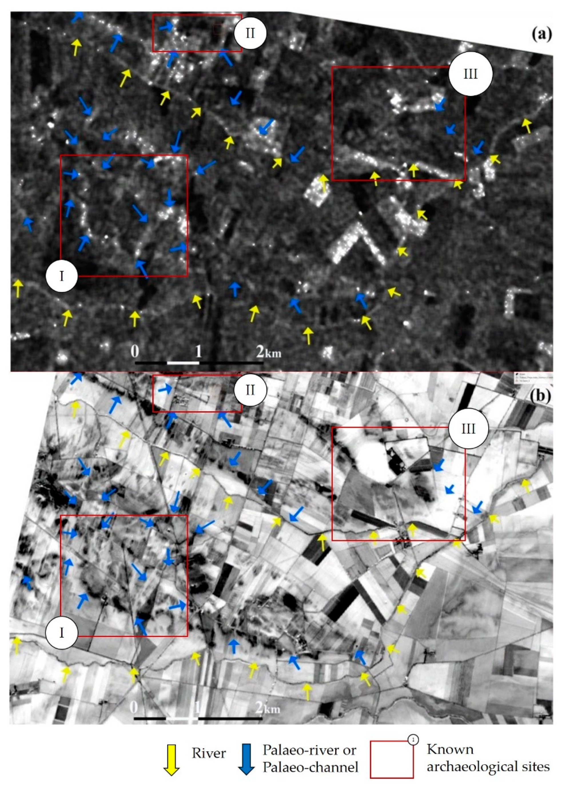
In addition, the ability to identify macro-elements of the ancient landscape was used on the comparison of known data present in previous archaeological and remote sensing studies applied to the province of Foggia [36,37,38,39,40,66,67,68,69] and S-1 data. The SAR data were used with S-2 data to trace the network of palaeo-rivers, communication routes, and Neolithic settlements, using as a test-area the area north-west of Foggia, known for the presence of ancient remains [66] (Figure 8).
Comparing S-1 and S-2 data, it is possible to clearly observe the palaeo-hydrographic features from S-1 (Figure 8a), due to changes in the moisture content, and the same palaeo-hydrographic features from the soil map (Figure 8b) obtained from S-2 [58] due to changes in moisture content and also probably due to soil organic nutrients.
The importance of an integrated approach of S-1 and S-2 for archaeology has been seen in the comparison of Sentinel data with high-resolution data on Google Earth (Figure 9).
For the same scene, a very high-resolution image from Google Earth (Figure 9d) acquired in the same month (October), but different year (2014), did not exhibit any indicators of palaeo-environmental and archaeological features.
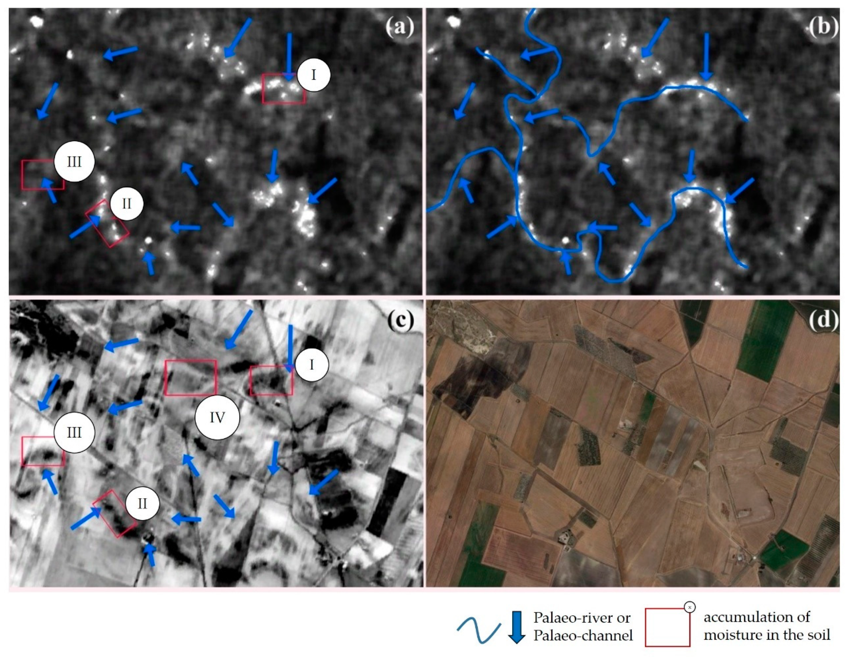
The comparison between the S-1 and S-2 scenes, evidence generally in correspondence of dark marks from S-2, corresponded with clear tone marks from S-1 (Figure 9I–III). However, in some cases, the tone of the features were inverted, appearing with light grey from S-2, and dark grey from S-1 (Figure 9IV).
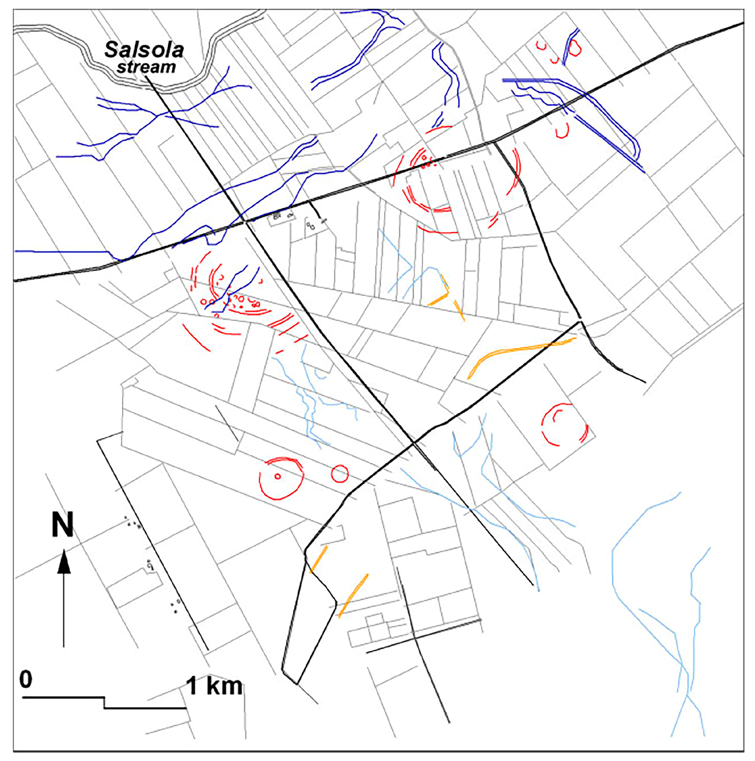
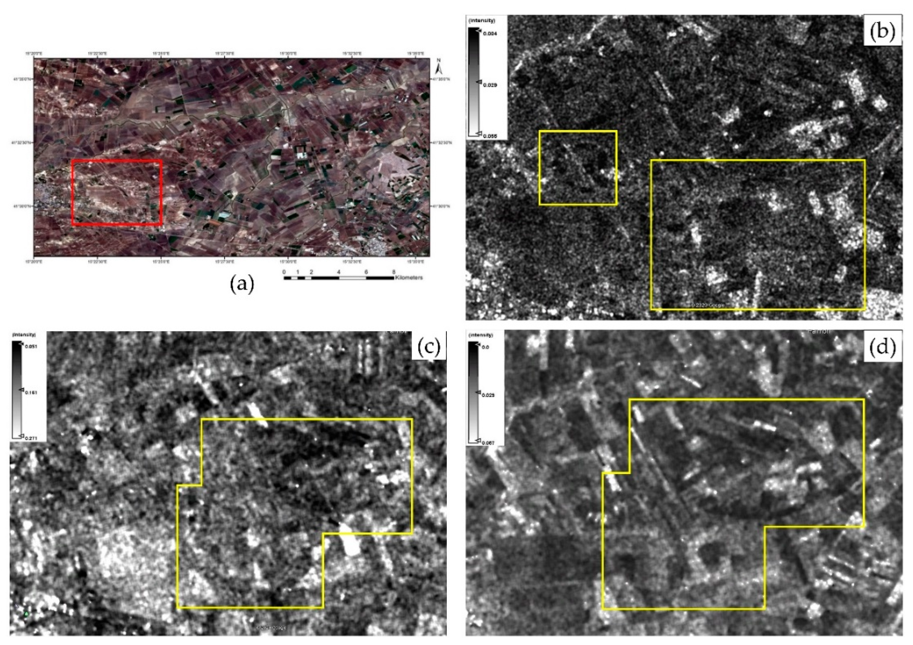
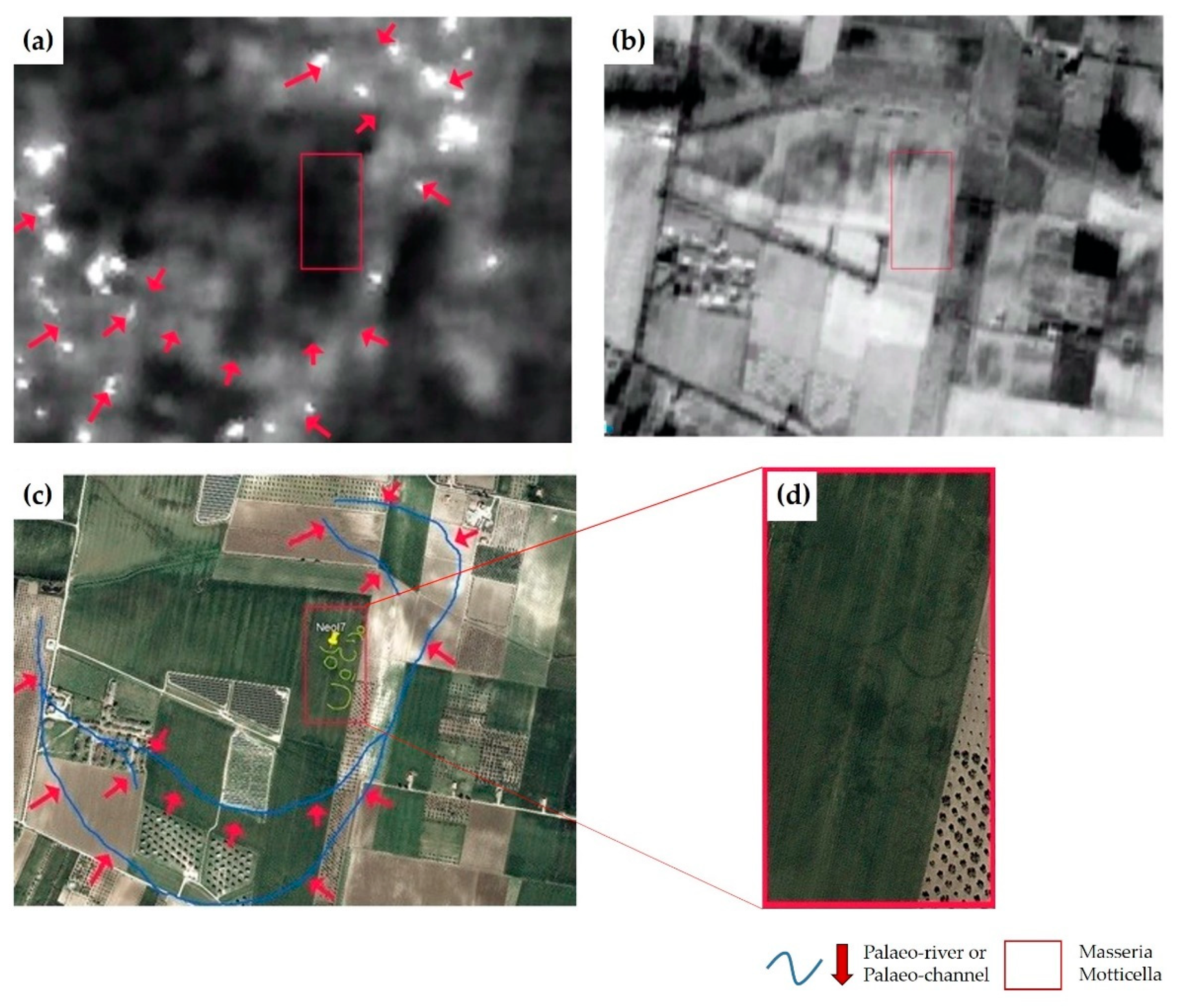
In other cases (Figure 10a,b), the brightest signal was not due to the presence of palaeo-rivers but likely due to the roughness of the soil. However, the integration of the Sentinel’s data with Google Earth data (Figure 10c) has allowed us to discover that the curvilinear palaeo-channel (characterized by two branches) goes around a Neolithic site, which is characterized by the circular features typical of the Neolithic settlements in this area.
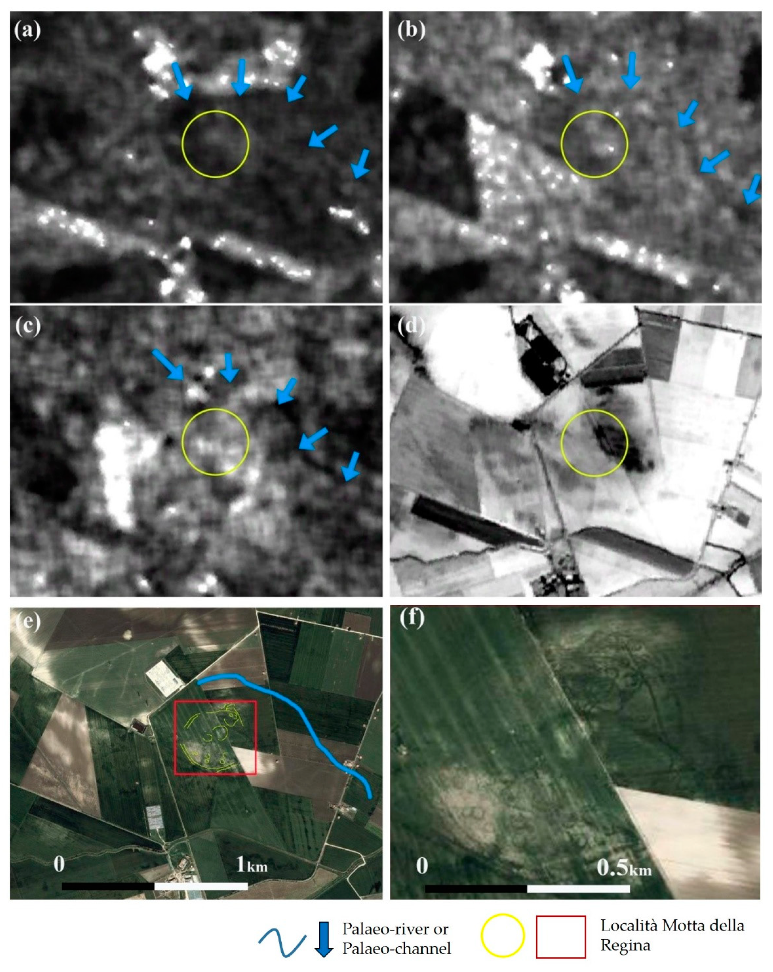
The behavior of the SAR signal in the identification of the palaeo-channel has proven to change depending on diverse factors. In addition to those already mentioned, the penetration capability and the depth of the buried palaeo-channel played a fundamental role. Likely due to the depth that is greater than the expected penetration capability, that the C-band waves were completely absorbed and the backscatter was very low: similar to the “radar river” behavior observed in deserted areas [67].
This behavior was observed for the area of Motta la Regina (Figure 8III and Figure 11). Contrary to what is generally observed for other sites (Figure 8I,II, Figure 9 and Figure 10), in these images, the palaeo-channels were characterized by a darker grey tone.
The great anthropogenic impact of the Neolithic trenched sites on the territory left visible traces, due to the abundant storage of moisture inside trenches and ditches, which make it possible to hypothesize the existence of new archaeological sites, also in accordance with the bibliography about the relationship between Neolithic sites, communication routes, and water resources (Figure 8).
The area represented in Figure 12 is located north of Foggia and is very close to the ancient city of Arpi. According to previous observations on already known archaeological sites (Figure 6, Figure 7, Figure 8, Figure 9 and Figure 10), the data suggest the presence of (i) Neolithic settlements in diverse locations, characterized by large circular or subcircular ditches; and (ii) roads and canals [23,24,25,26,27,28,29]. These elements are visible in the comparison of Figure 12b–d. The PCA from [58] mainly highlights the features left by roads and palaeo-channels. The same features are visible in the S-1 images more than in the RGB of 20 October 2019. The capability of SAR data to highlight elements of the ancient landscape, such as roads and rivers, is certainly useful in the identification of archaeological sites. In fact, settlements are often located along communication routes or water-courses for easy access to resources. As shown in Figure 12b–d, III, in the center of the image, ditches and streets are clearly visible in both the S-1-2 and S-1 images. In this case, there is a very articulated road system, which develops along two directions: a south-north road and an east-west road that crosses a trenched site, visible from the dark outline.
Features in Figure 12, evident in both the VH and VV SAR polarizations, are due to the combined effects of moisture and penetration capability of S-1 that are present and conditioned by the soil grain size and, above all, soil moisture content. In particular, concerning specifically the soil moisture, results from studies [64] conducted in several geographic areas, showed that VV enables better estimation of soil moisture compared with VH.
4. Discussion
The analysis of S-1 SAR data, according to what is described in the archaeological bibliography, aerial archaeology research, and remote sensing studies in the Foggia [36,37,38,39,40,66,67,68,69] area, proved useful for the identification of features of archaeological interest and for the identification of elements of the ancient landscape. However, as shown in Figure 6 and the following, the results are not always optimal for archaeological research and are closely related to several factors including (i) the type of buried evidence; (ii) sensor acquisition mode; and (iii) weather and soil conditions.
Buried remains or elements with a high impact on the landscape (rivers, roads, ditches, etc.) are more visible when they tend to retain soil moisture and are large enough to be appreciated with the use of S-1 SAR and its spatial resolution.
However, other factors deserve further discussion. In Section 4.1 and Section 4.2, the results are discussed in relation to the acquisition mode (ascending or descending orbit of the satellite) and the meteorological data that influenced the identification of the elements of archaeological interest within the multitemporal series of images.
4.1. Identification the Impact of Ascending/Descending Acquisition Modes
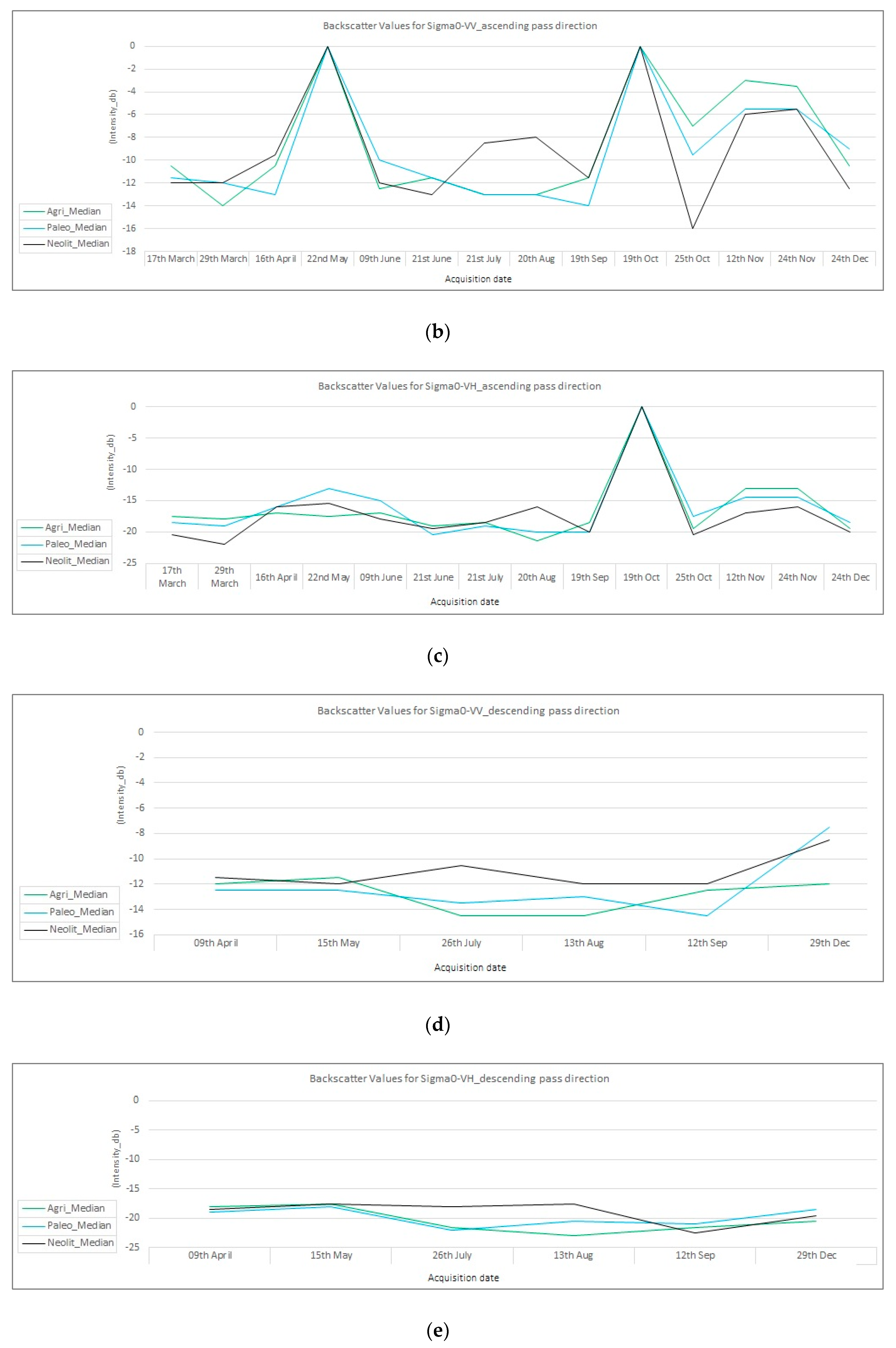
To better understand the intra-year variations in the visibility of the archaeological proxy indicators, the SAR data were first analyzed for the whole 2019 year (Table A2, Table A3, Table A4 and Table A5), considering, along with the VV/VH polarizations, the impact of ascending/descending acquisition modes over features related to known areas, such as agricultural areas, palaeo-river, and buried Neolithic settlements, as shown in Figure 13a–d. If we focalized on the single date acquisition, it was clear that according to the period of the year, both ascending and descending acquisitions enabled the discrimination of the diverse targets, and, if we analyzed one by one the single date acquisitions, the ascending tracks could be preferred because they are characterized by the higher backscattered coefficients that are due to the lowest incidence angle. As a whole, the best discrimination of the diverse considered targets is April and October, as evident from (Figure 13a–f) and also from the comparison made between the 2019 multi-dates S-1 and S-2 data set.
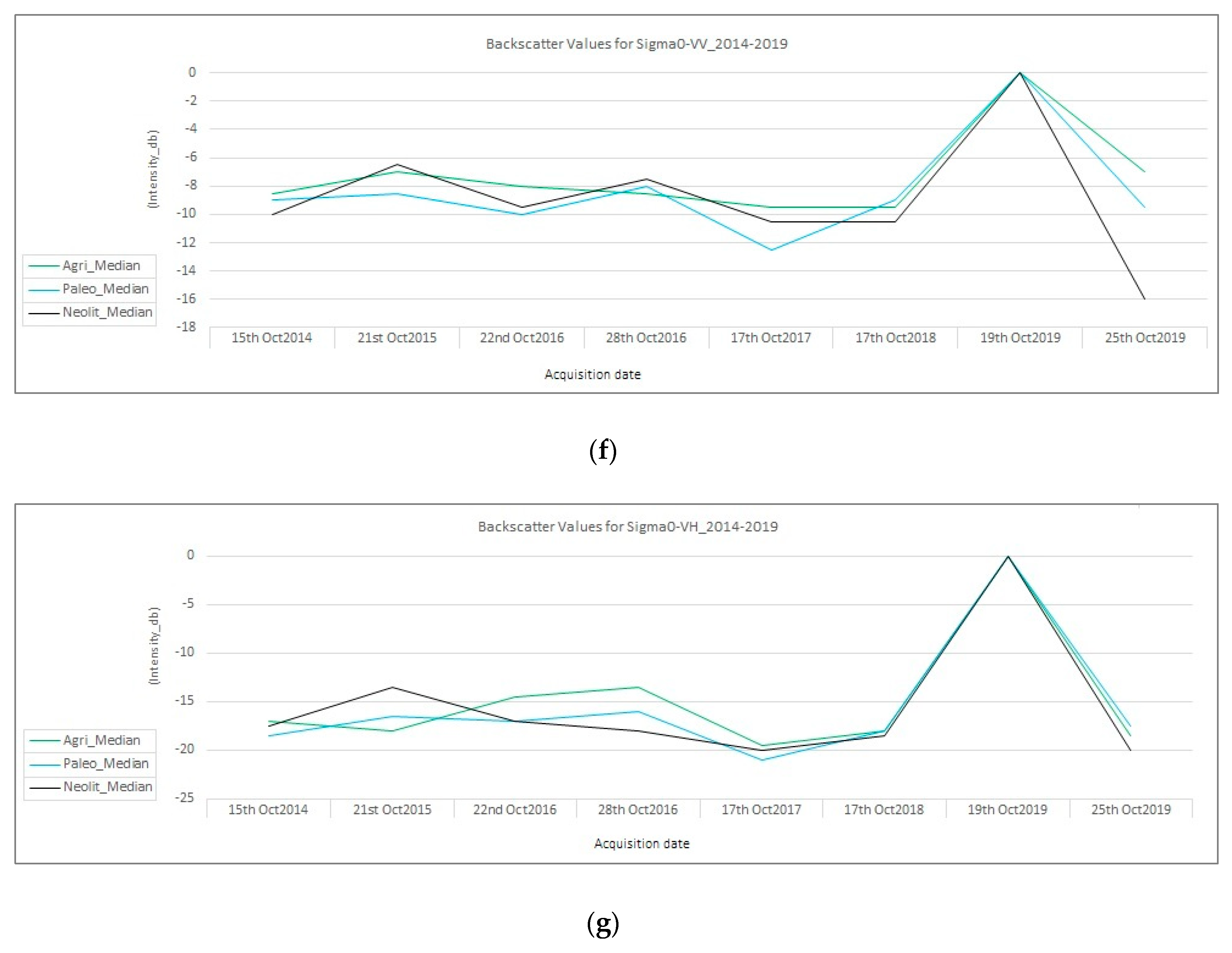
In the same context, SAR data for 2014, 2015, 2016, 2017, 2019, and 2019 were analyzed along with the VV/VH polarizations for the month of October (see Table in Appendix A and Figure 13f,g), which is considered the best time for extracting some buried shapes (Figure 13a,e,f). As a whole, the analysis performed herein suggested that:
- ✓
- ✓
- Secondly, considering that radar imaging outputs are influenced by the radar system itself, in terms of angles, viewing geometry (ascending or descending), and polarization,
- ○
- both ascending and descending modes appeared acceptable; however, we selected the ascending mode acquisition, as it is characterized by higher backscattering values due to the lower view angle compared to the descending pass, and;
- ○
- both VV and VH polarizations were suitable to enhance soil moisture and, in turn, archaeological marks; however, VV appeared more suitable.
4.2. Sentinel 1 Multiyear (2014–2019) Data Analyses
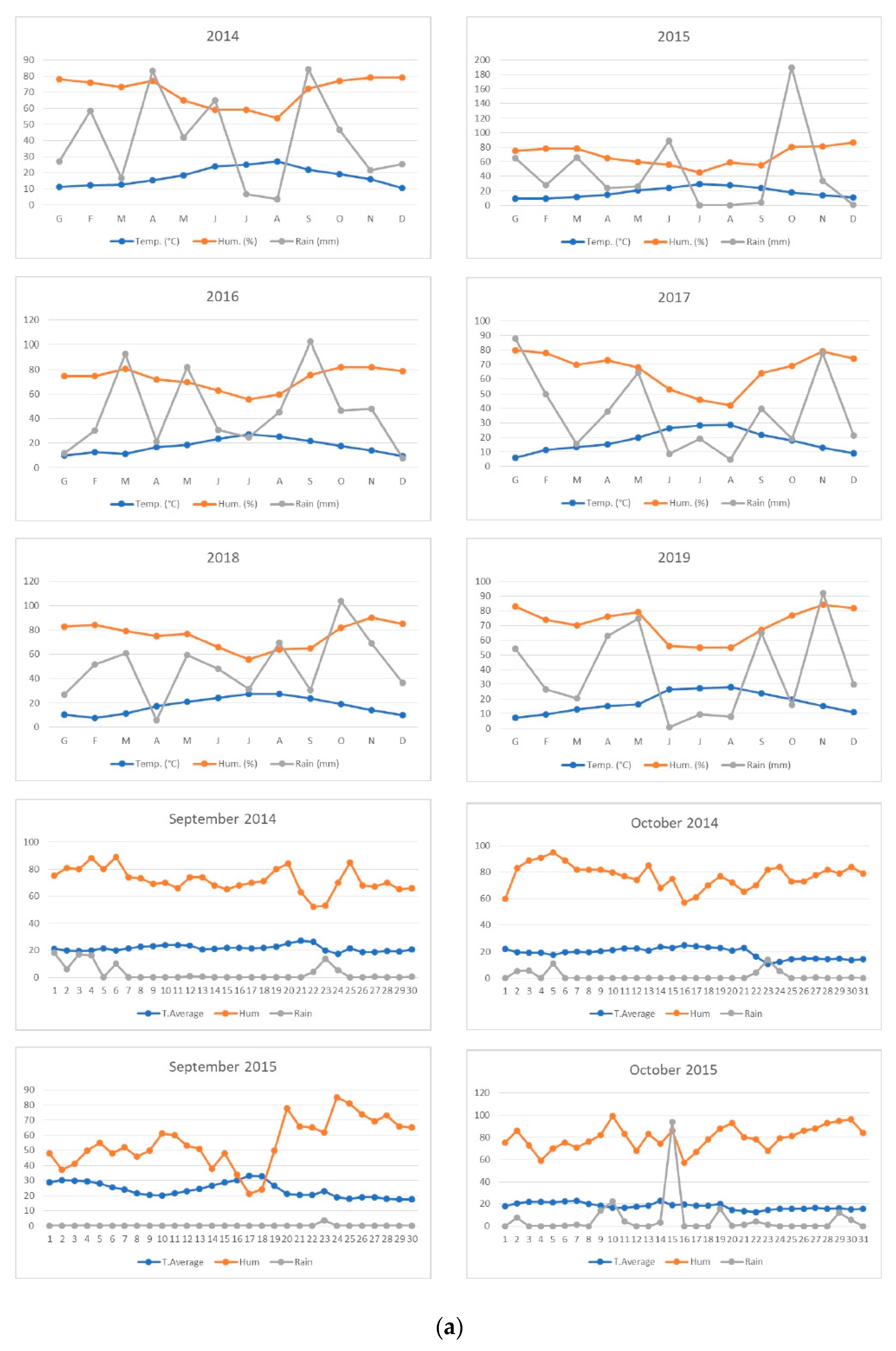
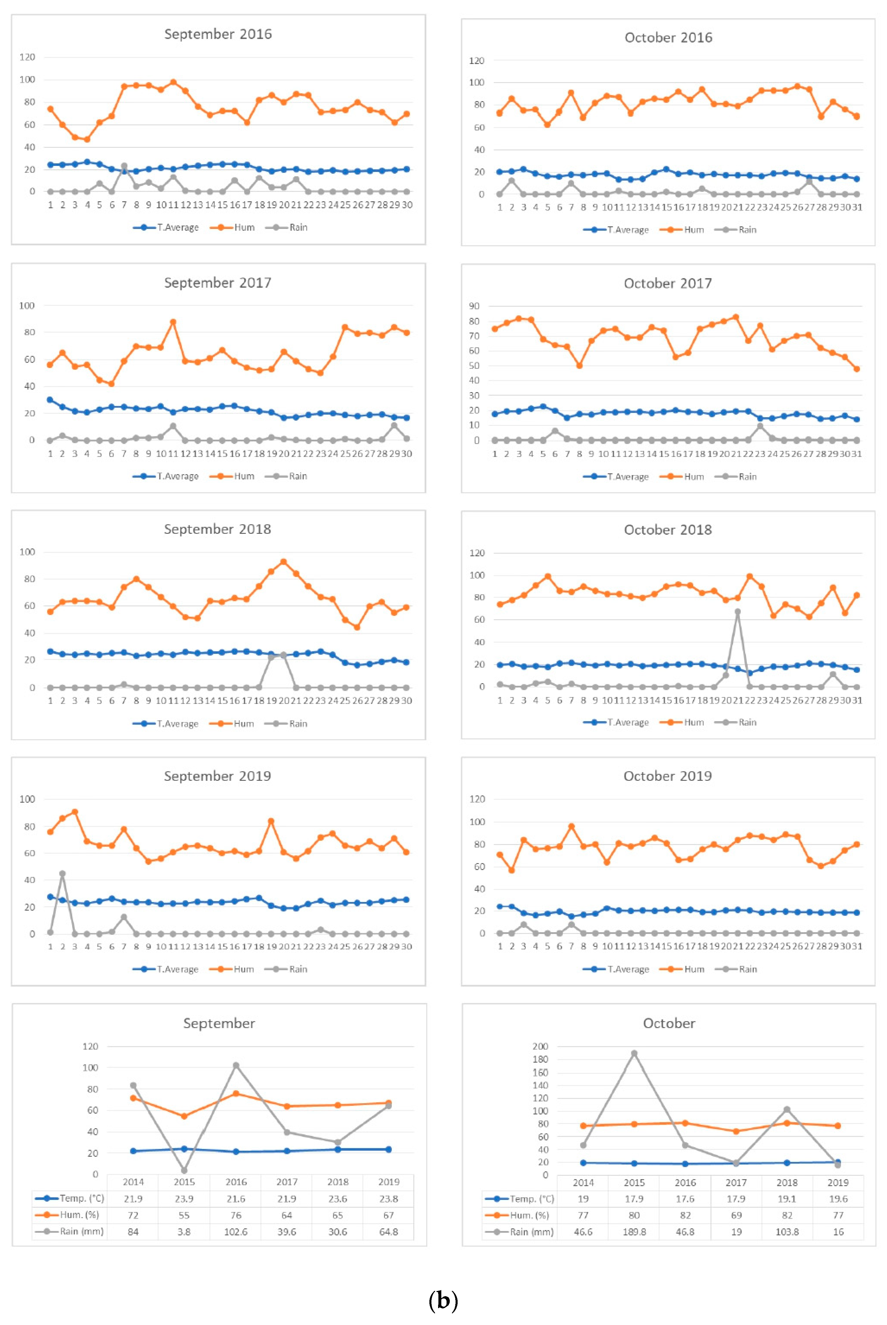
Outputs from the multiyear (2014–2019) data analysis highlighted that, in the study area, the highest capability of SAR Sentinel 1 in capturing archaeological proxy indicators was observed during summer and autumn. This is linked to the characteristics of the area in terms of the vegetation types and crop phenology, along with the impact of the meteorological conditions on the soil moisture content. To consider the contribution of soil moisture, we analyzed the SAR data coupled with the data on rain precipitation acquired from the meteorological stations in the areas and available from the Protezione Civile of the Apulia Region [71] (Figure 14a,b).
A comparative analysis of Figure 13 and Figure 14 suggests that the reason why the most appropriate months (July to November) obtained good results in S-1 was linked with the long duration of drying (with little of rains) and the higher SAR backscatter related to the agriculture land. In the study area, mainly cultivated with cereals (grain), the season of summer and autumn were characterized by a low presence of vegetation, which made the visibility of the soil and damp marks easier; thus, the best period to capture these archaeological marks is the month of October.
5. Conclusions
This study aimed to test the capability of Sentinel-1 Radar data in the identification and imaging of the subtle features linked to the palaeo-landscape and ancient human-induced transformation of the landscape in the Mediterranean environment.
The SAR data were difficult to understand and certainly less immediate than the S-2 optical sensor, especially in the detection of archaeological sites. In order to understand the SAR data of S-1, the results of the analysis were compared with information on the archaeological sites already known in the literature [36,37,38,39,40,66,67,68,69]. This comparison allowed a process of learning and understanding of the S-1 SAR data and the simultaneous use of S-2 and ancillary data to support and validate the diverse hypotheses. Of course, this approach was made possible by the rich archaeological documentation already produced for the area of study from research institutions and universities (see Section 2.1 and Section 3). The identification of sites from validated data, as in the case of the linear and circular features visible in Figure 7 [65] or Figure 11 [66], allowed us to understand which features were related to Neolithic settlements and to hypothesize, based on this experience, the existence of new archaeological sites as in Figure 12.
However, the visibility of the proxy indicators related to the palaeo-environmental and archaeological features, as described, depends on a number of factors, including (i) the presence of micro-topographical features; (ii) changes in the moisture content; and (iii) variation of crop growth and soil nutrients. These factors vary from one season to another and are dependent on the meteorological conditions, land use, and pedological and geological characteristics [2,21].
For these reasons, investigations based on time series are important to analyze and characterize the intra- and inter-year variability in the visibility of subtle features linked to the palaeo-landscape. To this aim, a significant test area (larger than 200 km2) was selected in the Foggia Province (South of Italy) and investigated using a time series of 2014–2019 for S-1 data to analyze and characterize the (i) intra- and inter-year variability in the visibility of features linked to the palaeo-landscape, along with the (ii) impact of different acquisitions (ascending and descending) modes and polarization VV/VH.
As a whole, the results from these investigations indicated that (i) the best period for the visibility of the archaeological proxy indicator was summer and autumn as already determined for optical data [68]; (ii) both ascending and descending modes well captured the subtle features of interest; however, the ascending mode was preferable as it was characterized by higher backscattering values. In more detail, on the basis of our analysis, as expected being that archaeological features are not permanent signals, several specific acquisitions from the S-1A, B data (captured on 15 October 2014, 21 October 2015, 28 October 2016, 17 October 2017, 17 October 2018, 19 October 2019, and 25 October 2019) provided the highest visibility of the subtle palaeo-landscape features. On the basis of these S-1 acquisitions, several new anomalies of potential archaeological interest were identified. In particular, palaeo-rivers and palaeo-channels along with ditches in shape and size “compatible” with the Neolithic era were detected and successfully compared with independent studies and data (such as the air photographs acquired by the RAF during the Second World War).
Insights into the strong connection between Neolithic settlements, roads, and palaeo-rivers/palaeo-channels were evident and highlighted by our S-1 based findings (see Figure 8, Figure 9, Figure 10, Figure 11 and Figure 12). This is very important, not only for the study areas but also because this opens new potential S-1 applications and research lines. In fact, the results from our investigations clearly highlighted the high potentiality of S-1 in the identification of the very subtle features linked to palaeo-landscape features and ancient anthropogenic transformation in vegetated areas, such as in the Mediterranean ecosystems. This is a very important result, considering that, since the early assessment of the potentiality of SAR in archaeology, satellite L-band SAR sensors SAR data were traditionally used for subsurface imaging in arid regions to reconstruct the palaeo-landscape, given the ability of longer wavelengths to penetrate more deeply into sand [72]. This study demonstrated the high capabilities of shorter-wavelengths (in particular the S-1 C-band sensor) in subsurface imaging in vegetated areas of the Mediterranean ecosystems, and these results offer important new insights in the application of SAR for palaeo-environmental investigations:
- ✓
- First, the capability of S-1 to detect traces of past environment and landscape with particular reference to ancient surface water rivers highlighted that can S-1 data can provide a major contribution in archaeological investigations considering that rivers are and were crucial to past human activity and are, therefore, considered important targets of archaeological prospection;
- ✓
- Secondly, the successful results of this investigation can be replicated in different geographic areas considering the free worldwide availability of S-1 data along with data processing tools;
- ✓
- Thirdly, considering that the main critical, challenging aspect of the use of SAR in archaeology is a lack of correspondence between the great amount of spaceborne SAR data (as in the case of S-1) and effective methods to extract information linked to past human activity, this paper contributes in providing a methodological approach to exploit S-1 data in archaeological investigations.
As a whole, the results from our investigations highlighted that S-1 data can provide a major contribution in archaeological investigations and also overcome the limits of passive optical data: active sensors are able, to some extent, to “penetrate” vegetation and soil and unveil important targets of archaeological prospection, such as palaeo-rivers and palaeo-channels, that are currently not evident in the modern landscape and from the optical data. The detection of palaeo-hydrography is fundamental for the study of human history and the first human settlements, in the Neolithic, or earlier, which depends on the understanding of the local river dynamics and hydrological variability [36,37,38,39,40,66,67,68,69,73,74,75,76]. Palaeo-hydrography can inform us regarding the ancient site’s occupation in the prehistoric period as water is, and was, the most immediate requisite element for human survival. Therefore, the identification of palaeo-rivers and palaeo-channels, along with ancient roads, can suitably provide information regarding buried lost settlements, which generally require the data of large areas to investigate.
Once proven that S-1 can be used for the identification of remains of archaeological interest and palaeo-environmental elements, there are many possible future developments, some of which have been already successfully tested with other types of data (e.g., TerraSAR-X, COSMO-SkyMed, or Gaofen-1), such as the identification, the extraction, or the classification of linear and sub-linear features [18,19,77,78,79].
The approach proposed herein provides a great advantage to easily identify large features (such as palaeo-channels and ditches) or linear routes, and to narrow down surface surveys to be further investigated using very high-resolution data and/or geophysical prospections, thus reducing the time of analysis and, potentially, the cost for excavations. This type of approach provides a tool, in addition to those already used in the Earth Observation techniques and in combination with some of them (e.g., S-2, Landsat TM, or PRISMA Satellite data), at the service of landscape archaeology, regardless of the area of application. On the other hand, knowledge of the territory, anywhere in the world, opens up opportunities for the protection, discovery, and preservation of cultural heritage.
Author Contributions
There were three main contributions in the current research article; the archaeological view, remote sensing data analysis, and writing of the manuscript. N.M., N.A., and A.E. provided the archaeological view. The maps and remote sensing imagery were analyzed by R.L., A.E., N.M., and N.A. The manuscript was written by A.E., N.A., N.M., and R.L. The last version of the article was revised by N.M. and R.L. All authors have read and agreed to the published version of the manuscript.
Funding
The authors would like to declare that the research received no external funding and the research activities were performed by the author’s research centers.
Acknowledgments
Special thanks to NAIS and CNR-IMAA for funding N.A. at the University of Basilicata. The authors would like to thank CNR-ISPC along with the National Authority for Remote sensing and Space science (NARSS) at Cairo, Egypt for supporting the research activities. The authors would like to thank Protezione Civile Puglia for the weather data provided for this research.
Conflicts of Interest
The authors would like to hereby certify that there were no conflicts of interest in the data collection, processing, and post-processing, the writing and revision of the manuscript, nor in the decision to publish the manuscript results.
Appendix A

Table A1.
Backscatter values for the Sentinel 1 2019 Sigma0-VV ascending pass direction.
| Date | Agriculture 1 | Agriculture 2 | Median | Palaeo-river 1 | Palaeo-river 2 | Median | Neolithic 1 | Neolithic 2 | Median |
|---|---|---|---|---|---|---|---|---|---|
| 17 March | −9.0 | −12.0 | −10.5 | −12.0 | −10.0 | −11.5 | −13.0 | −11.0 | −12.0 |
| 29 March | −11.0 | −17.0 | −14.0 | −12.0 | −12.0 | −12.0 | −15.0 | −9.0 | −12.0 |
| 16 April | −7.0 | −14.0 | −10.5 | −11.0 | −15.0 | −13.0 | −10.0 | −9.0 | −9.5 |
| 22 May | Nan | Nan | Nan | Nan | Nan | Nan | Nan | Nan | Nan |
| 9 June | −11.0 | −14.0 | −12.5 | −10.0 | −10.0 | −10.0 | −14.0 | −10.0 | −12.0 |
| 21 June | −9.0 | −14.0 | −11.5 | −10.0 | −12.0 | −11.5 | −14.0 | −12.0 | −13.0 |
| 21 July | −12.0 | −14.0 | −13.0 | −13.0 | −13.0 | −13.0 | −9.0 | −8.0 | −8.5 |
| 20 August | −12.0 | −14.0 | −13.0 | −13.0 | −13.0 | −13.0 | −9.0 | −7.0 | −8.0 |
| 19 September | −9.0 | −14.0 | −11.5 | −13.0 | −15.0 | −14.0 | −12.0 | −11.0 | −11.5 |
| 19 October | Nan | Nan | Nan | Nan | Nan | Nan | Nan | Nan | Nan |
| 25 October | −6.0 | −8.0 | −7.0 | −11.0 | −8.0 | −9.5 | −18.0 | −14.0 | −16.0 |
| 12 November | −2.0 | −4.0 | −3.0 | −6.0 | −5.0 | −5.5 | −10.0 | −2.0 | −6.0 |
| 24 November | −3.0 | −4.0 | −3.5 | −7.0 | −4.0 | −5.5 | −9.0 | −2.0 | −5.5 |
| 24 December | −10.0 | −11.0 | −10.5 | −10.0 | −8.0 | −9.0 | −13.0 | −12.0 | −12.5 |
Table A2.
Backscatter values for the Sentinel 1 2019 Sigma0-VH ascending pass direction.
| Date | Agriculture 1 | Agriculture 2 | Median | Palaeo-river 1 | Palaeo-river 2 | Median | Neolithic 1 | Neolithic 2 | Median |
|---|---|---|---|---|---|---|---|---|---|
| 17 March | −18.0 | −17.0 | −17.5 | −17.0 | −20.0 | −18.5 | −19.0 | −22.0 | −20.5 |
| 29 March | −18.0 | −18.0 | −18.0 | −19.0 | −19.0 | −19.0 | −20.0 | −24.0 | −22.0 |
| 16 April | −15.0 | −19.0 | −17.0 | −13.0 | −19.0 | −16.0 | −14.0 | −18.0 | −16.0 |
| 22 May | −17.0 | 18.0 | −17.5 | −11.0 | −15.0 | −13.0 | 16.0 | 15.0 | −15.5 |
| 9 June | −15.0 | −19.0 | −17.0 | −13.0 | −17.0.0 | −15.0 | −20.0 | −16.0 | −18.0 |
| 21 June | −15.0 | −23.0 | −19.0 | −18.0 | −23.0 | −20.5 | −23.0 | −16.0 | −19.5 |
| 21 July | −17.0 | −20.0 | −18.5 | −17.0 | −21.0 | −19.0 | −19.0 | −17.0 | −18.5 |
| 20 August | −19.0 | −24.0 | −21.5 | −17.0 | −23.0 | −20.0 | −18.0 | −14.0 | −16.0 |
| 19 September | −17.0 | −20.0 | −18.5 | −19.0 | −21.0 | −20.0 | −20.0 | −20.0 | −20.0 |
| 19 October | Nan | Nan | Nan | Nan | Nan | Nan | Nan | Nan | Nan |
| 25 October | −19.0 | −20.0 | −19.5 | −17.0 | −18.0 | −17.5 | −20.0 | −21.0 | −20.5 |
| 12 November | −11.0 | −15.0 | −13.0 | −15.0 | −14.0 | −14.5 | −19.0 | −15.0 | −17.0 |
| 24 November | −13.0 | −13.0 | −13.0 | −16.0 | −13.0 | −14.5 | −18.0 | −14.0 | −16.0 |
| 24 December | −18.0 | −21.0 | −19.5 | −18.0 | −19.0 | −18.5 | −18.0 | −22.0 | −20.0 |
Table A3.
Backscatter values for the Sentinel 1 2019 Sigma0-VV descending pass direction.
| Date | Agriculture 1 | Agriculture 2 | Median | Palaeo-river 1 | Palaeo-river 2 | Median | Neolithic 1 | Neolithic 2 | Median |
|---|---|---|---|---|---|---|---|---|---|
| 9 April | −8.0 | −16.0 | −12.0 | −10.0 | −15.0 | −12.5 | −14.0 | −9.0 | −11.5 |
| 15 May | −10.0 | −13.0 | −11.5 | −12.0 | −13.0 | −12.5 | −14.0 | −10.0 | −12.0 |
| 26 July | −13.0 | −16.0 | −14.5 | −12.0 | −15.0 | −13.5 | −11.0 | −10.0 | −10.5 |
| 13 August | −15.0 | −14.0 | −14.5 | −13.0 | −13.0 | −13.0 | −13.0 | −11.0 | −12.0 |
| 12 September | −10.0 | −15.0 | −12.5 | −13.0 | −16.0 | −14.5 | −12.0 | −12.0 | −12.0 |
| 29 December | −11.0 | −13.0 | −12.0 | −7.0 | −8.0 | −7.5 | −8.0 | −9.0 | −8.5 |
Table A4.
Backscatter values for the Sentinel 1 2019 Sigma0-VH descending pass direction.
| Date | Agriculture 1 | Agriculture 2 | Median | Palaeo-river 1 | Palaeo-river 2 | Median | Neolithic 1 | Neolithic 2 | Median |
|---|---|---|---|---|---|---|---|---|---|
| 9 April | −17.0 | −19.0 | −18.0 | −17.0 | −21.0 | −19.0 | −15.0 | −22.0 | −18.5 |
| 15 May | −17.0 | −18.0 | −17.5 | −17.0 | −19.0 | −18.0 | −17.0 | −18.0 | −17.5 |
| 26 July | −20.0 | −23.0 | −21.5 | −19.0 | −25.0 | −22.0 | −21.0 | −14.0 | −18.0 |
| 13 August | −22.0 | −24.0 | −23.0 | −19.0 | −22.0 | −20.5 | −20.0 | −15.0 | −17.5 |
| 12 September | −19.0 | −24.0 | −21.5 | −18.0 | −24.0 | −21.0 | −23.0 | −22.0 | −22.5 |
| 29 December | −19.0 | −22.0 | −20.5 | −18.0 | −19.0 | −18.5 | −18.0 | −21.0 | −19.5 |
Table A5.
Backscatter values for the Sentinel 1 2014, 2015, 2016, 2017, 2018, and 2019 Sigma0-VV polarization.
Table A5.
Backscatter values for the Sentinel 1 2014, 2015, 2016, 2017, 2018, and 2019 Sigma0-VV polarization.
| Date | Agriculture 1 | Agriculture 2 | Median | Palaeo-river 1 | Palaeo-river 2 | Median | Neolithic 1 | Neolithic 2 | Median |
|---|---|---|---|---|---|---|---|---|---|
| 15 October 2014 | −7.0 | −10.0 | −8.5 | −10.0 | −8.0 | −9.0 | −9.0 | −11.0 | −10.0 |
| 21 October 2015 | −5.0 | −9.0 | −7.0 | −10.0 | −7.0 | −8.5 | −6.0 | −7.0 | −6.5 |
| 22 October 2016 | −7.0 | −9.0 | −8.0 | −10.0 | −10.0 | −10.0 | −11.0 | −8.0 | −9.5 |
| 28 October 2016 | −7.0 | −10.0 | −8.5 | −9.0 | −7.0 | −8.0 | −8.0 | −7.0 | −7.5 |
| 17 October 2017 | −9.0 | −10.0 | −9.5 | −14.0 | −11.0 | −12.5 | −12.0 | −9.0 | −10.5 |
| 17 October 2018 | −9.0 | −10.0 | −9.5 | −9.0 | −9.0 | −9.0 | −10.0 | −11.0 | −10.5 |
| 19 October 2019 | Nan | Nan | Nan | Nan | Nan | Nan | Nan | Nan | Nan |
| 25 October 2019 | −6.0 | −8.0 | −7.0 | −10.0 | −9.0 | −9.5 | −17.0 | −15.0 | −16.0 |
Table A6.
Backscatter values for the Sentinel 1 2014, 2015, 2016, 2017, 2018, and 2019 Sigma0−VH polarization.
Table A6.
Backscatter values for the Sentinel 1 2014, 2015, 2016, 2017, 2018, and 2019 Sigma0−VH polarization.
| Date | Agriculture 1 | Agriculture 2 | Median | Palaeoriver 1 | Palaeoriver 2 | Median | Neolithic 1 | Neolithic 2 | Median |
|---|---|---|---|---|---|---|---|---|---|
| 15 October 2014 | −15.0 | −19.0 | −17.0 | −17.0 | −20.0 | −18.5 | −17.0 | −18.0 | −17.5 |
| 21 October 2015 | −15.0 | −21.0 | −18.0 | −18.0 | −15.0 | −16.5 | −12.0 | −15.0 | −13.5 |
| 22 October 2016 | −15.0 | −14.0 | −14.5 | −18.0 | −16.0 | −17.0 | −16.0 | −18.0 | −17.0 |
| 28 October 2016 | −16.0 | −11.0 | −13.5 | −19.0 | −13.0 | −16.0 | −17.0 | −19.0 | −18.0 |
| 17 October 2017 | −18.0 | −21.0 | −19.5 | −22.0 | −20.0 | −21.0 | −17.0 | −23.0 | −20.0 |
| 17 October 2018 | −17.0 | −19.0 | −18.0 | −18.0 | −18.0 | −18.0 | −19.0 | −18.0 | −18.5 |
| 19 October 2019 | Nan | Nan | Nan | Nan | Nan | Nan | Nan | Nan | Nan |
| 25 October 2019 | −19.0 | −18.0 | −18.5 | −16.0 | −19.0 | −17.5 | −20.0 | −20.0 | −20.0 |
References
- Lasaponara, R.; Masini, N. Remote sensing in archaeology: From visual data interpretation to digital data manipulation. In Satellite Remote Sensing. A New Tool for Archaeology; Lasaponara, R., Masini, N., Eds.; Springer: Dordrecht, The Netherlands, 2012; pp. 3–16. [Google Scholar]
- Masini, N.; Lasaponara, R. Sensing the Past from Space: Approaches to Site Detection. In Sensing the Past. From Artifact to Historical Site; Masini, N., Soldovieri, F., Eds.; Springer: Dordrecht, The Netherlands, 2017; pp. 23–60. [Google Scholar]
- Agapiou, A. Remote sensing heritage in a petabyte-scale: Satellite data and heritage Earth Engine© applications. Int. J. Digit. Earth 2017, 10, 85–102. [Google Scholar] [CrossRef] [Green Version]
- Luo, L.; Wang, X.; Guo, H.; Lasaponara, R.; Zong, X.; Masini, N.; Wang, G.; Shi, P.; Khatteli, H.; Fulong, C.; et al. Airborne and spaceborne remote sensing for archaeological and cultural heritage applications: A review of the century (1907–2017). Remote Sens. Environ. 2019, 232, 111280. [Google Scholar] [CrossRef]
- Hemsley, J.; Cappellini, V.; Stanke, G. (Eds.) Digital Applications for Cultural and Heritage Institutions; Routledge: London, UK, 2017. [Google Scholar]
- Elfadaly, A.; Attia, W.; Lasaponara, R. Monitoring the Environmental Risks Around Medinet Habu and Ramesseum Temple at West Luxor, Egypt, Using Remote Sensing and GIS Techniques. J. Archaeol. Method Theory 2018, 25, 587–610. [Google Scholar] [CrossRef]
- Elfadaly, A.; Attia, W.; Qelichi, M.M.; Murgante, B.; Lasaponara, R. Management of Cultural Heritage Sites Using Remote Sensing Indices and Spatial Analysis Techniques. Surv. Geophys. 2018, 39, 1347–1377. [Google Scholar] [CrossRef]
- Elfadaly, A.; Wafa, O.; Abouarab, M.A.; Guida, A.; Spanu, P.G.; Lasaponara, R. Geo-Environmental Estimation of Land Use Changes and Its Effects on Egyptian Temples at Luxor City. ISPRS Int. J. Geo Inf. 2017, 6, 378. [Google Scholar] [CrossRef] [Green Version]
- Lasaponara, R.; Murgante, B.; Elfadaly, A.; Qelichi, M.M.; Shahraki, S.Z.; Wafa, O.; Attia, W. Spatial open data for monitoring risks and preserving archaeological areas and landscape: Case studies at Kom el Shoqafa, Egypt and Shush, Iran. Sustainability 2017, 9, 572. [Google Scholar] [CrossRef] [Green Version]
- Stewart, C. Detection of Archaeological Residues in Vegetated Areas Using Satellite Synthetic Aperture Radar. Remote Sens. 2017, 9, 118. [Google Scholar] [CrossRef] [Green Version]
- Agapiou, A.; Alexakis, D.D.; Hadjimitsis, D.G. Potential of Virtual Earth Observation Constellations in Archaeological Research. Sensors 2019, 19, 4066. [Google Scholar] [CrossRef] [Green Version]
- Tzouvaras, M.; Kouhartsiouk, D.; Agapiou, A.; Danezis, C.; Hadjimitsis, D.G. The Use of Sentinel-1 Synthetic Aperture Radar (SAR) Images and Open-Source Software for Cultural Heritage: An Example from Paphos Area in Cyprus for Mapping Landscape Changes after a 5.6 Magnitude Earthquake. Remote Sens. 2019, 11, 1766. [Google Scholar] [CrossRef] [Green Version]
- Gaffney, V.L.; Thomson, K.; Fitch, S. (Eds.) Mapping Doggerland: The Mesolithic Landscapes of the Southern North Sea; Archaeopress: London, UK, 2007. [Google Scholar]
- Elfadaly, A.; Abouarab, M.A.R.; El Shabrawy, R.R.M.; Mostafa, W.; Wilson, P.; Morhange, C.; Silverstein, J.; Lasaponara, R. Discovering Potential Settlement Areas around Archaeological Tells Using the Integration between Historic Topographic Maps, Optical, and Radar Data in the Northern Nile Delta, Egypt. Remote Sens. 2019, 11, 3039. [Google Scholar] [CrossRef] [Green Version]
- Lasaponara, R.; Masini, N. Satellite synthetic aperture radar in archaeology and cultural landscape: An overview. Archaeol. Prospect. 2013, 20, 71–78. [Google Scholar] [CrossRef]
- Paillou, P. Mapping Palaeohydrography in Deserts: Contribution from Space-Borne Imaging Radar. Water 2017, 9, 194. [Google Scholar] [CrossRef]
- Chen, F.; Masini, N.; Yang, R.; Milillo, P.; Feng, D.; Lasaponara, R. A Space View of Radar Archaeological Marks: First Applications of COSMO-SkyMed X-Band Data. Remote Sens. 2015, 7, 24–50. [Google Scholar] [CrossRef] [Green Version]
- Chen, F.; Masini, N.; Liu, J.; You, J.; Lasaponara, R. Multi-frequency satellite radar imaging of cultural heritage: The case studies of the Yumen Frontier Pass and Niya ruins in the Western Regions of the Silk Road Corridor. Int. J. Digit. Earth 2016, 9, 1224–1241. [Google Scholar] [CrossRef]
- Lasaponara, R.; Masini, N.; Pecci, A.; Perciante, F.; Escot, D.P.; Rizzo, E.; Scavone, M.; Sileo, M. Qualitative evaluation of COSMO SkyMed in the detection of earthen archaeological remains: The case of Pachamacac (Peru). J. Cult. Herit. 2017, 23, 55–62. [Google Scholar] [CrossRef]
- Conversa, G.; Lazzizera, C.; Bonasia, A.; Cifarelli, S.; Losavio, F.; Sonnante, G.; Elia, A. Exploring on-farm agro-biodiversity: A study case of vegetable landraces from Puglia region (Italy). Biodivers. Conserv. 2020, 29, 747–770. [Google Scholar] [CrossRef]
- Ciarangi, N.; Loiacono, F.; Moretti, M. ISPRA, Note Illustrative della Carta Geologica Italiana; Foglio 408: Foggia, Italy, 2011. [Google Scholar]
- Gallo, D.; Ciminale, M.; Becker, H.; Masini, N. Remote sensing techniques for reconstructing a vast Neolithic settlement in Southern Italy. J. Archaeol. Sci. 2009, 36, 43–50. [Google Scholar] [CrossRef]
- Whitehouse, R. The Neolithic pottery sequence in southern Italy. Proc. Prehist. Soc. 2014, 35, 267–310. [Google Scholar] [CrossRef]
- Longhena, M.; Robb, J. (Eds.) The Early Mediterranean Village. Agency, Material Culture, and Social Change in Neolithic Italy; Cambridge University Press: Cambridge, UK, 2007. [Google Scholar]
- Pluciennik, M. Radiocarbon determinations and the mesolithic-neolithic transition in southern Italy. J. Mediterr. Archaeol. 1998, 10, 115–150. [Google Scholar] [CrossRef]
- Acquafredda, P.; Muntoni, I.M. Obsidian from Pulo di Molfetta (Bari, Southern Italy): Provenance from Lipari and first recognition of a Neolithic sample from Monte Arci (Sardinia). J. Archaeol. Sci. 2008, 35, 947–955. [Google Scholar] [CrossRef]
- Bradford, J.; Williams-Hunt, P.R. Siticulosa Apulia. Antiquity 1946, 20, 191–200. [Google Scholar] [CrossRef]
- Bradford, J.S.P. The Apulia expedition: An interim report. Antiquity 1950, 24, 84–94. [Google Scholar] [CrossRef]
- Mills, S.; Macklin, M.; Mirea, P. Encounters in the watery realm: Early to mid-Holocene geochronologies of Lower Danube human–river interactions. In The Neolithic of Europe: Papers in Honor of Alasdair Whittle; Bickle, P., Hofmann, D., Pollard, J., Eds.; Oxbow Books: Oxford, UK, 2018; pp. 35–46. [Google Scholar]
- Battarbee, R.W.; Gasse, F.; Stickley, C.E. (Eds.) Past Climate Variability through Europe and Africa; Springer: Dordrecht, The Netherlands, 2004. [Google Scholar]
- Tozzi, C. Contributo alla conoscenza del villaggio neolitico di Ripa Tetta (Lucera). In 6th Convegno sulla Preistoria-Protostoria-Storia della Daunia: San Severo, Italy, 14–16 Dicembre 1984; Mundi, B., Gravina, A., Eds.; Archeoclub di San Severo: San Severo, Italy, 1984; pp. 11–20. [Google Scholar]
- Biancofiore, F. Note di antropologia economica delle comunità neolitiche della Puglia centrosettentrionale. In 5th Convegno sulla Preistoria-Protostoria-Storia della Daunia: San Severo, Italy, 9–11 Dicembre 1983; Mundi, B., Gravina, A., Eds.; Archeoclub di San Severo: San Severo, Italy, 1983; pp. 25–33. [Google Scholar]
- Cassano, S.M. La diffusione del Neolitico in Puglia. In Convegno sulla Preistoria-Protostoria-Storia della Daunia: San Severo, 23–25 Novembre 1979; Archeoclub di San Severo: San Severo, Italy, 1979; pp. 63–71. [Google Scholar]
- Gravina, A. Caratteri del Neolitico medio-finale nella Daunia centro-meridionale. In Proceedings of the 6th Convegno sulla Preistoria-Protostoria-Storia della Daunia, San Severo, Italy, 14–16 December 1984; Mundi, B., Gravina, A., Eds.; Archeoclub di San Severo: San Severo, Italy, 1984; pp. 21–41. [Google Scholar]
- Gravina, A. Masseria Istituto di Sangro un insediamento del neolitico medio-finale nella Daunia. In Proceedings of the 8th Convegno Nazionale sulla Preistoria-Protostoria-Storia della Daunia, San Severo, Italy, 12–14 December 1986; Archeoclub di San Severo: San Severo, Italy, 1986; pp. 25–33. [Google Scholar]
- Whitehouse, R.D. The chronology of the Neolithic ditched settlements of the Tavoliere and the Ofanto Valley. In Rethinking the Italian Neolithic. Special Issue; Pearce, M., Whitehouse, R.D., Eds.; Accordia Research Institute: London, UK, 2013; pp. 57–78. [Google Scholar]
- Caldara, M.; Fiorentino, G.; Primavera, M. Hidden Nolithic Landscsapes in Apulian Region. In Hidden Landscapes of Mediterranean Europe. Cultural and Methodological Biases in Pre- and Protohistoric Landscape Studies, Proceedings of the international meeting, Siena, Italy, 25–27 May 2007; van Leusen, M., Pizziolo, G., Sarti, L., Eds.; BAR International Series: Oxford, UK, 2011; pp. 183–191. [Google Scholar]
- Fiorentino, G.; Caldara, M.; De Santis, V.; D’Oronzo, C.; Muntoni, I.M.; Simone, O.; Primavera, M.; Radina, F. Climate changes and human-environment interactions in the Apulia region of southeastern Italy during the Neolithic period. Holocene 2013, 23, 1297–1316. [Google Scholar] [CrossRef]
- Danise, M.; Masini, N.; Biscione, M.; Lasaponara, R. Predictive modeling for preventive Archaeology: Overview and case study. Cent. Eur. J. Geosci. 2014, 6, 42–55. [Google Scholar] [CrossRef]
- CartApulia. Available online: http://www.cartapulia.it/ (accessed on 2 May 2020).
- Esa data. Available online: https://scihub.copernicus.eu/dhus/#/home (accessed on 4 February 2020).
- Alaska Satellite Facility. Available online: https://search.asf.alaska.edu/#/ (accessed on 4 February 2020).
- Usman, F.; Ibrahim, E. Detecting Seasonal Extent of Inundated Area of River Body in Banyuasin Regency Using Radar Data of Sentinel-1A. In Proceedings of the AWAM International Conference on Civil Engineering, Penang, Malaysia, 21–22 August 2019; Springer: Cham, Switzerland, 2019; pp. 771–784. [Google Scholar]
- Filipponi, F. Sentinel-1 GRD Preprocessing Workflow. Multidiscip. Digit. Publ. Inst. Proc. 2019, 18, 11. [Google Scholar] [CrossRef] [Green Version]
- Fletcher, K. (Ed.) SENTINEL 1: ESA‘s Radar Observatory Mission for GMES Operational Services; European Space Agency: Paris, France, 2012. [Google Scholar]
- Mancon, S.; Guarnieri, A.M.; Tebaldini, S. Sentinel-1 precise orbit calibration and validation. In Proceedings of the FRINGE 2015, Roma, Italy, 23–27 March 2015; pp. 1–4. [Google Scholar]
- Park, J.W.; Korosov, A.A.; Babiker, M.; Sandven, S.; Won, J.S. Efficient thermal noise removal for Sentinel-1 TOPSAR cross-polarization channel. IEEE Trans. Geosci. Remote Sens. 2017, 56, 1555–1565. [Google Scholar] [CrossRef]
- Schubert, A.; Small, D.; Meier, E.; Miranda, N.; Geudtner, D. Spaceborne SAR product geolocation accuracy: A Sentinel-1 update. In Proceedings of the 2014 IEEE Geoscience and Remote Sensing Symposium, Quebec City, QC, Canada, 13–18 July 2014; pp. 2675–2678. [Google Scholar]
- Twele, A.; Cao, W.; Plank, S.; Martinis, S. Sentinel-1-based flood mapping: A fully automated processing chain. Int. J. Remote Sens. 2016, 37, 2990–3004. [Google Scholar] [CrossRef]
- Sentinel1 Post Processing Using Some Algorithms. Available online: https://sentinel.esa.int/web/sentinel/level-1-post-processing-algorithms (accessed on 4 February 2020).
- Veloso, A.; Mermoz, S.; Bouvet, A.; Le Toan, T.; Planells, M.; Dejoux, J.F.; Ceschia, E. Understanding the temporal behavior of crops using Sentinel-1 and Sentinel-2-like data for agricultural applications. Remote Sens. Environ. 2017, 199, 415–426. [Google Scholar] [CrossRef]
- Chang, L. Analysis of Sentinel-1 SAR Data for Mapping Standing Water in the Twente Region. Master’s Thesis, Specialization, Faculty of Geo-Information Science and Earth Observation of the University of Twente, Enschende, The Netherlands, February 2016. [Google Scholar]
- Sar-pre-processing. Available online: https://buildmedia.readthedocs.org/media/pdf/multiply-sar-preprocessing/get_to_version_0.4/multiply-sar-pre-processing.pdf (accessed on 2 May 2020).
- Abdurahman Bayanudin, A.; Heru Jatmiko, R. Orthorectification of Sentinel-1 SAR (Synthetic Aperture Radar) Data in Some Parts Of South-eastern Sulawesi Using Sentinel-1 Toolbox. In IOP Conference Series: Earth and Environmental Science; IOP Publishing Ltd.: Bristol, UK, 2016; Volume 47, No. 1; p. 012007. [Google Scholar]
- Adriansen, H.K. Land reclamation in Egypt: A study of life in the new lands. Geoforum 2009, 40, 664–674. [Google Scholar] [CrossRef] [Green Version]
- Belenguer-Plomer, M.A.; Tanase, M.A.; Fernandez-Carrillo, A.; Chuvieco, E. Burned area detection and mapping using Sentinel-1 backscatter coefficient and thermal anomalies. Remote Sens. Environ. 2019, 233, 111–345. [Google Scholar] [CrossRef]
- Rüetschi, M.; Schaepman, M.E.; Small, D. Using multitemporal sentinel-1 c-band backscatter to monitor phenology and classify deciduous and coniferous forests in northern switzerland. Remote Sens. 2018, 10, 55. [Google Scholar] [CrossRef] [Green Version]
- Abate, N.; Elfadaly, A.; Masini, N.; Lasaponara, R. Multitemporal 2016–2018 Sentinel-2 Data Enhancement for Landscape Archaeology: The Case Study of the Foggia Province, Southern Italy. Remote Sens. 2020, 12, 1309. [Google Scholar] [CrossRef] [Green Version]
- Bleuler, M.; Farina, R.; Francaviglia, R.; di Bene, C.; Napoli, R.; Marchetti, A. Modelling the impacts of different carbon sources on the soil organic carbon stock and CO2 emissions in the Foggia province (southern Italy). Agric. Syst. 2017, 157, 258–268. [Google Scholar] [CrossRef]
- Riley, D.N. New aerial reconnaissance in Apulia. Pap. Br. Sch. Rome 1992, 60, 291–307. [Google Scholar] [CrossRef]
- Malone, C. The Italian Neolithic: A synthesis of research. J. World Prehistory 2003, 17, 235–312. [Google Scholar] [CrossRef]
- Mazzucco, N.; Capuzzo, G.; Pannocchia, C.P.; Ibáñez, J.J.; Gibaja, J.F. Harvesting tools and the spread of the Neolithic into the Central-Western Mediterranean area. Quat. Int. 2018, 470, 511–528. [Google Scholar] [CrossRef]
- Skeates, R. The social dynamics of enclosure in the Neolithic of the Tavoliere, south-east Italy. J. Mediterr. Archaeol. 2000, 13, 155–188. [Google Scholar] [CrossRef]
- El Hajj, M.; Baghdadi, N.; Zribi, M.; Bazzi, H. Synergic use of Sentinel-1 and Sentinel-2 images for operational soil moisture mapping at high spatial resolution over agricultural areas. Remote Sens. 2017, 9, 1292. [Google Scholar] [CrossRef] [Green Version]
- Jones, G.D.B. Apulia. Volume I: Neolithic Settlement in the Tavoliere; Society of Antiquaries of London: London, UK, 1987. [Google Scholar]
- Guaitoli, M.; Cazzato, V. (Eds.) Lo Sguardo di Icaro. La Collezione dell ‘Aerofototeca Nazionale per la Conoscenza del Territorio; Campisano Editore: Roma, Italy, 2003. [Google Scholar]
- McCauley, J.F.; Schaber, G.G.; Breed, C.S.; Grolier, M.J.; Haynes, C.V.; Issawi, B.; Elachi, C.; Bloom, R. Subsurface valleys and geoarchaeology of the Eastern Sahara revealed by shuttle radar. Science 1982, 218, 1004–1020. [Google Scholar] [CrossRef]
- Masini, N.; Marzo, C.; Manzari, P.; Belmonte, A.; Sabia, C.; Lasaponara, R. On the characterization of temporal and spatial patterns of archaeological crop-marks. J. Cult. Herit. 2018, 32, 124–132. [Google Scholar] [CrossRef]
- Agapiou, A.; Lysandrou, V.; Lasaponara, R.; Masini, N. Study of the Variations of Archaeological Marks at Neolithic Site of Lucera, Italy Using High-Resolution Multispectral Datasets. Remote Sens. 2016, 8, 723. [Google Scholar] [CrossRef] [Green Version]
- Goffredo, R. Aerial archaeology in Daunia (northern Puglia, Italy). New research and developments. BAR Int. Ser. 2006, 1568, 541. [Google Scholar]
- Hydrological Annals for Puglia. Available online: https://protezionecivile.puglia.it/centro-funzionale-decentrato/rete-di-monitoraggio/annali-e-dati-idrologici-elaborati/annali-idrologici-parte-i-download/ (accessed on 4 February 2020).
- Wiig, F.; Harrower, M.J.; Brau, A.; Nathan, S.; Lehne, J.W.; Simo, K.M.; Sturm, J.O.; Trinder, J.; Dumitru, I.A.; Hensley, S.; et al. Mapping a Subsurface Water Channel with X-Band and C-Band Synthetic Aperture Radar at the Iron Age Archaeological Site of ‘Uqdat al-Bakrah (Safah), Oman. Geosciences 2018, 8, 334. [Google Scholar] [CrossRef] [Green Version]
- Sargent, A. Changing settlements location and subsistence in later prehistoric Apulia, Italy. Origini 2001, 23, 145–168. [Google Scholar]
- Whitehouse, N.J.; Kirleis, W. The world reshaped: Practices and impacts of early agrarian societies. J. Archaeol. Sci. 2014, 51, 1–11. [Google Scholar] [CrossRef]
- Whitehouse, N.J.; Schulting, R.J.; McClatchie, M.; Barratt, P.; McLaughlin, T.R.; Bogaard, A.; Colledge, S.; Marchant, R.; Gaffrey, J.; Bunting, M.J. Neolithic agriculture on the European western frontier: The boom and bust of early farming in Ireland. J. Archaeol. Sci. 2013, 51, 181–205. [Google Scholar] [CrossRef]
- Morter, J.; Robb, J. The Chora of Croton 1: The Neolithic Settlement at Capo Alfiere; University of Texas Press: Austin, TX, USA, 2012. [Google Scholar]
- Stewart, C.; Montanaro, R.; Sala, M.; Riccardi, P. Feature Extraction in the North Sinai Desert Using Spaceborne Synthetic Aperture Radar: Potential Archaeological Applications. Remote Sens. 2016, 8, 825. [Google Scholar] [CrossRef] [Green Version]
- Tapete, D.; Cigna, F. COSMO-SkyMed SAR for Detection and Monitoring of Archaeological and Cultural Heritage Sites. Remote Sens. 2019, 11, 1326. [Google Scholar] [CrossRef] [Green Version]
- Lou, L.; Bachagha, N.; Yao, Y.; Liu, C.; Shi, P.; Zhu, L.; Shao, J.; Wang, X. Identifying Linear Traces of the Han Dynasty Great Wall in Dunhuang Using Gaofen-1 Satellite Remote Sensing Imagery and the Hough Transform. Remote Sens. 2019, 11, 2711. [Google Scholar]
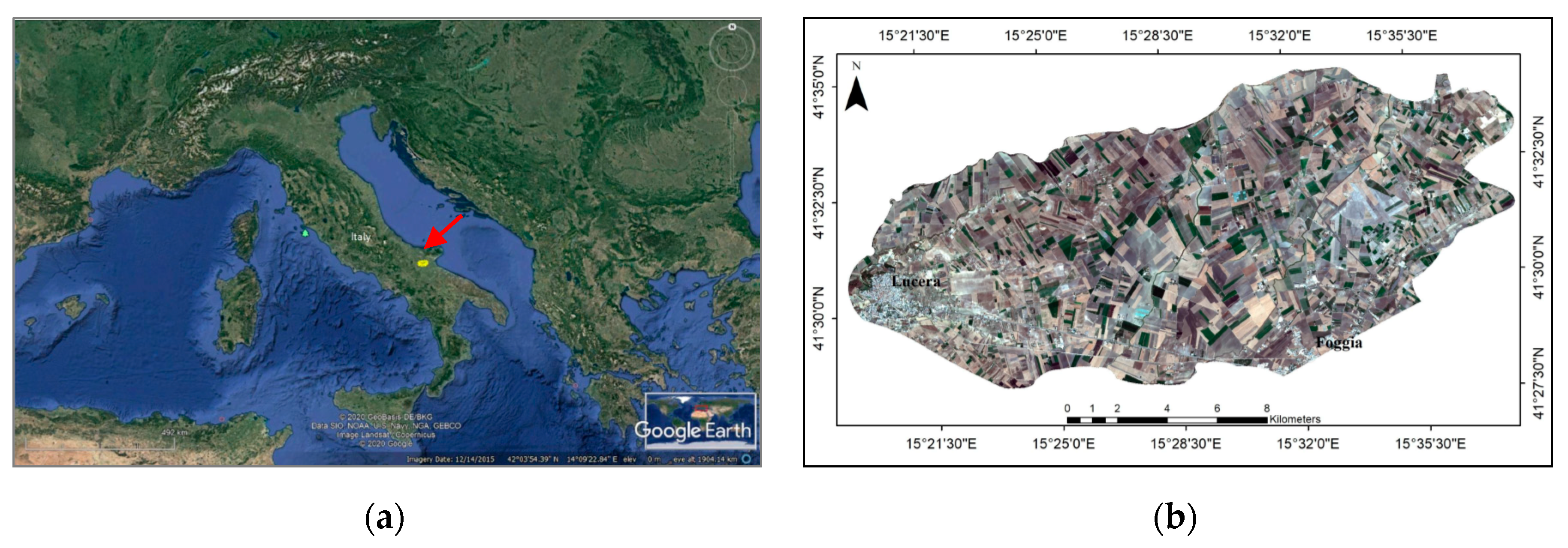
Figure 1.
Study area location: (a) Italy by Google Earth Pro image; (b) Study area by Sentinel-2A August 2019 (RGB 4,3,2).
Figure 1.
Study area location: (a) Italy by Google Earth Pro image; (b) Study area by Sentinel-2A August 2019 (RGB 4,3,2).

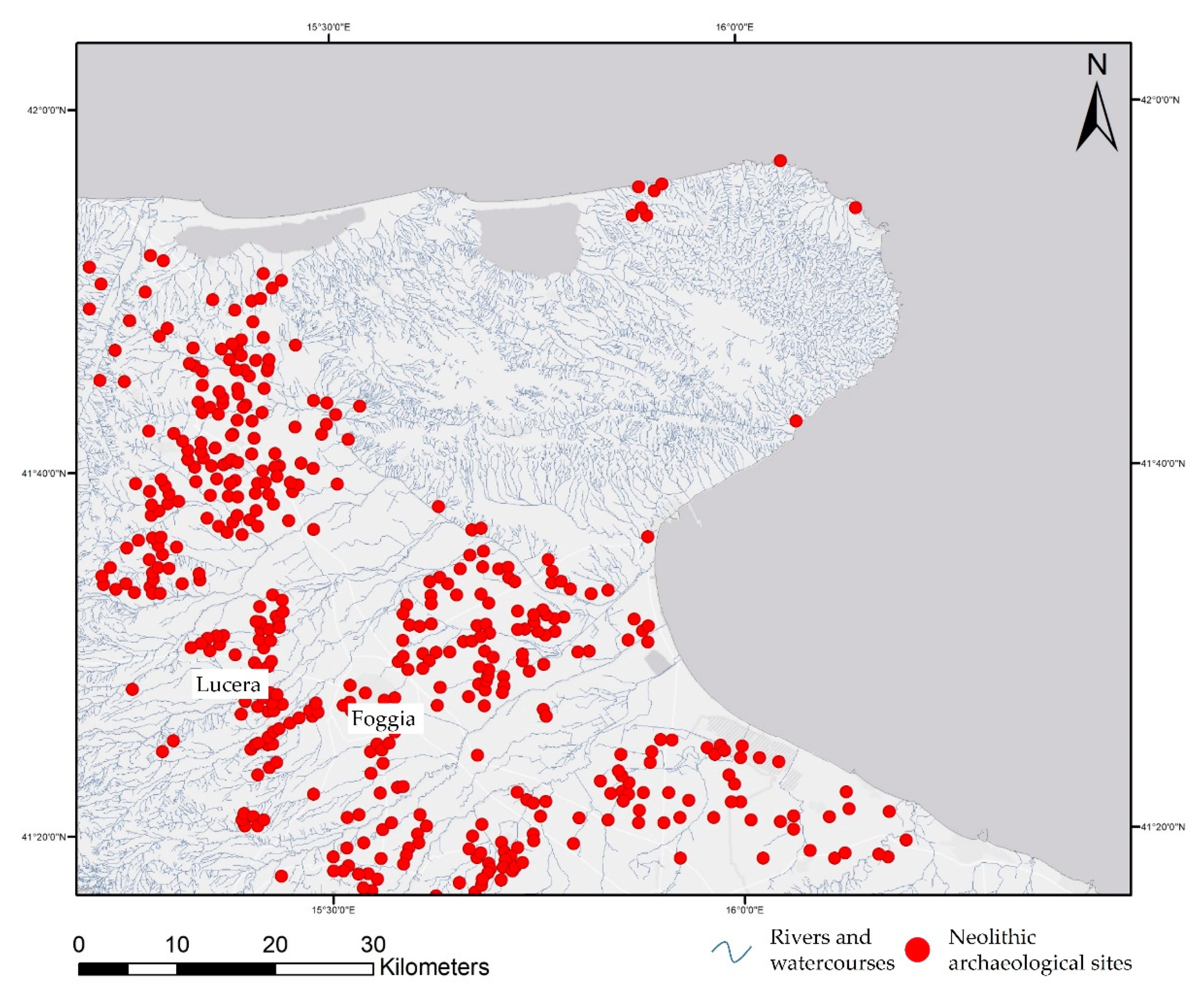
Figure 2.
Map of the distribution of Neolithic settlements in the province of Foggia, reworked by the authors starting from different bibliographic sources and WebGis CartApulia [36,39,40].

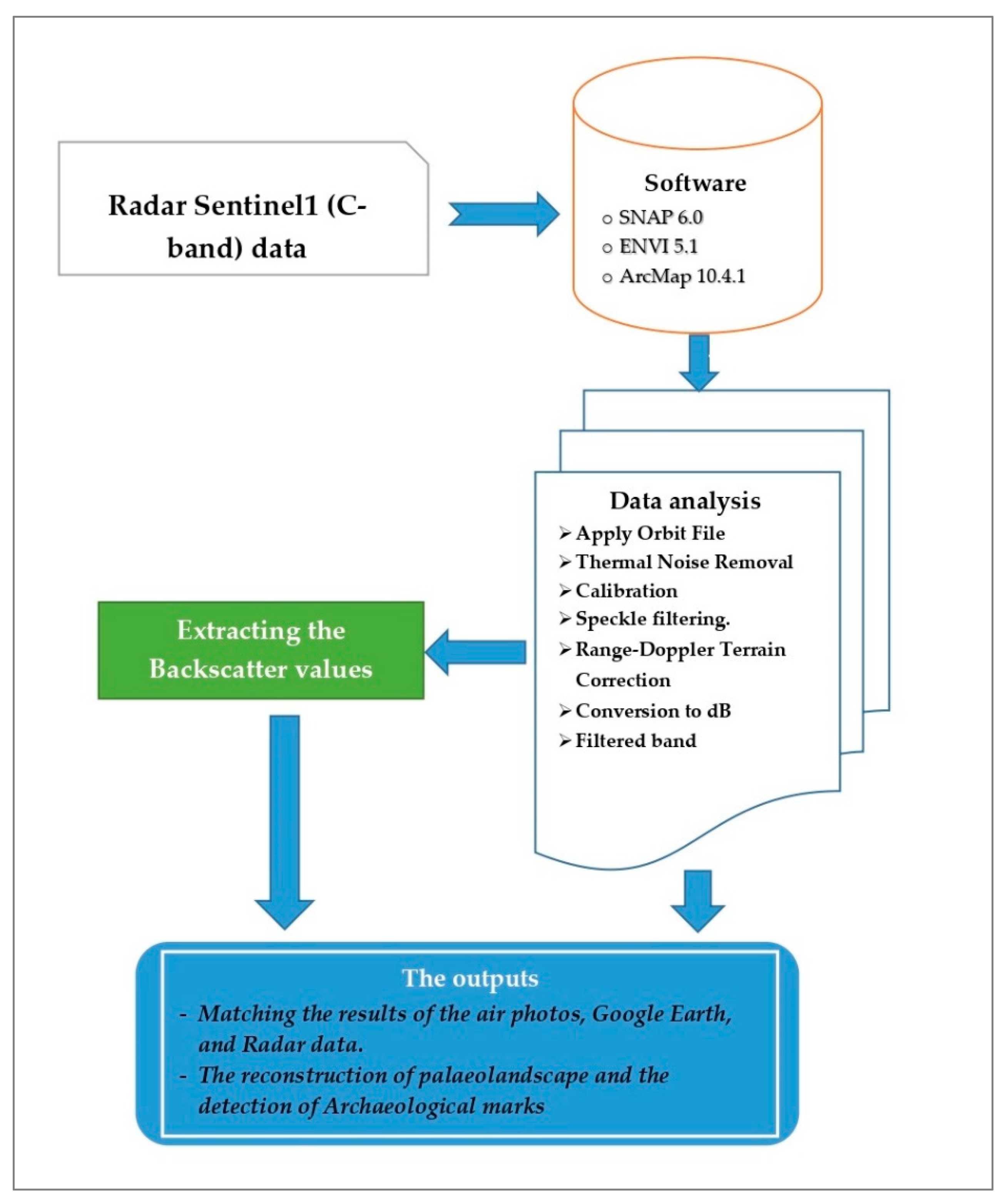
Figure 3.
The flowchart of the study, including the data, methods, and the results of the study.

Figure 4.
Study area by S-2 and S-1 satellite imagery: (a) S-2 image captured on 20 October 2019 (natural colors RGB 4,3,2); (b) S-2 image captured on 20 October 2019 (natural colors FCIR 8,4,3); (c) S-1 VV polarization captured on the 19th and (d) VH polarization captured on 19 October 2019.
Figure 4.
Study area by S-2 and S-1 satellite imagery: (a) S-2 image captured on 20 October 2019 (natural colors RGB 4,3,2); (b) S-2 image captured on 20 October 2019 (natural colors FCIR 8,4,3); (c) S-1 VV polarization captured on the 19th and (d) VH polarization captured on 19 October 2019.

Figure 5.
The analysed SAR data in October 2014, 2015, 2016, 2017, 2018, and 2019: (a) S-1 captured on 15 October 2014; (b) S-1 captured on 21 October 2015; (c) S-1 captured on 26 October 2016; (d) S-1 captured on 17 October 2017; (e) S-1 captured on 17 October 2018; (f) S-l1 captured on 19 October 2019. Yellow boxes are expected archaeological sites.

Figure 6.
Example of evidence of the ancient landscape and archaeological remains in Apulia: (i) blue lines represent palaeoriver; (ii) red lines represent the Neolithic settlements of Palmori and Schifata; (iii) orange lines represent roads; (iv) light blue lines represent hydromorphic marks related to an ancient marshy environment; (v) black and grey lines represent modern roads, channels and fields ([14], Figure 5).

Figure 7.
Known archaeological sites identifiable within the S-1 SAR data: (a) location of the zoom area east of Lucera (S-2, RGB, 20 October 2019); (b) Masseria Sarcone and Masseria Albani (S-1, 19 October 2019, Sigma_0 VH); (c) Masseria Villano (S-1, 28 October 2016, Sigma_0 VH); (d) Masseria Villano and Masseria Seggese (S-1, 28 October 2016, Sigma_0 VV) [65].

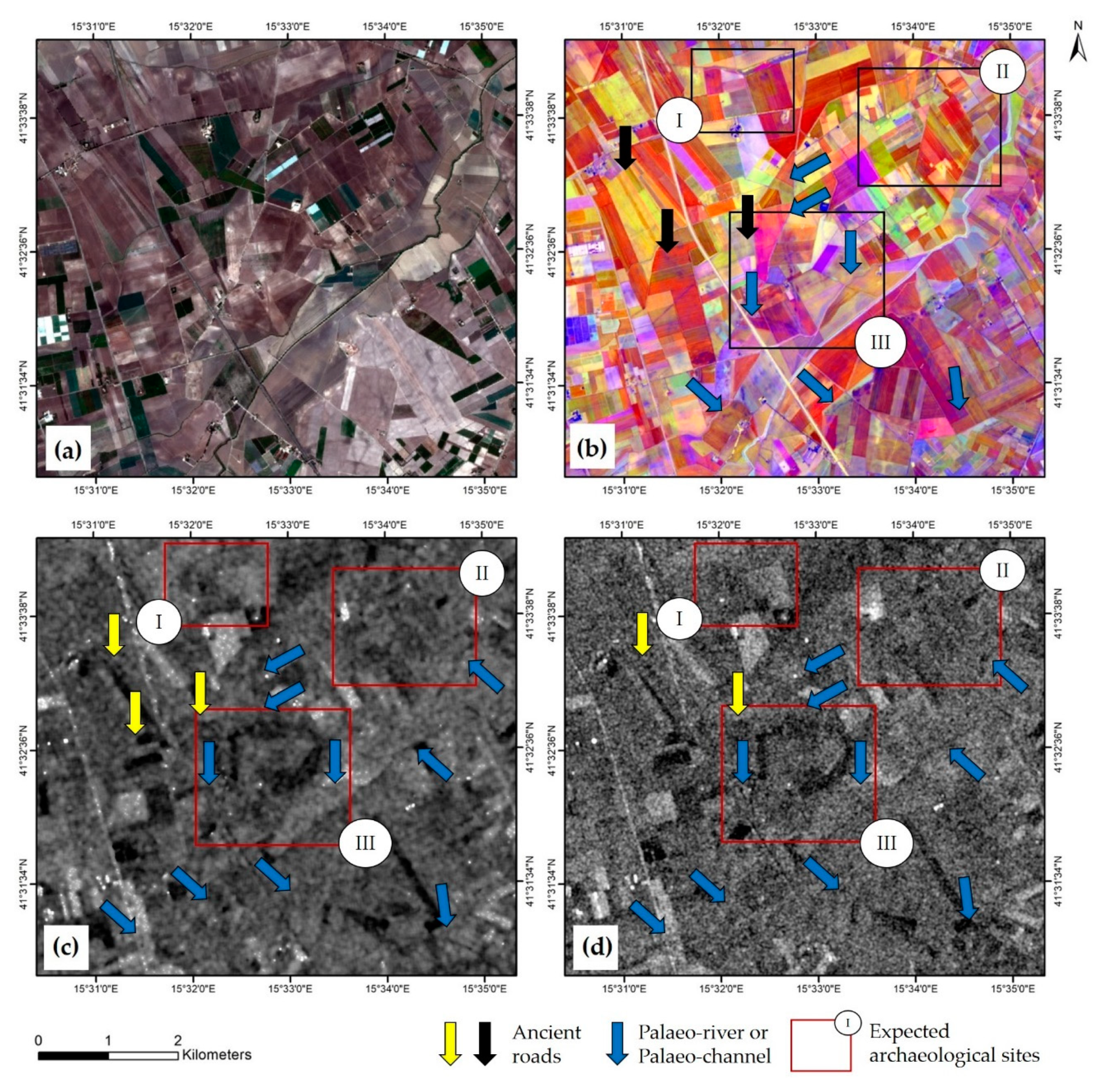
Figure 8.
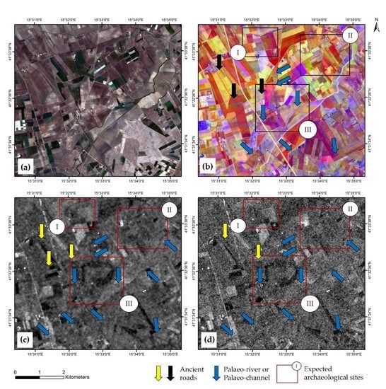
A palaeo-landscape including palaeo-rivers and palaeo-channels observed from: (a) VV S-1 data acquired on the 19 October 2019; (b) S-2 based soil map acquired on the 20 October 2019. The blue and yellow arrows indicate the palaeo-hydrographic and hydrographic features, observed from S-1 and S-2, respectively. The red numbered boxes indicate archaeological sites already known from bibliography and ancillary data, which are connected to a network of water-courses and roads: I. Località Ciamponetto (Neolithic and Roman settlements); II. Masseria Motticella (Neolithic settlement); III. Località Motta della Regina (neolithic settlement and medieval buildings) [66].
Figure 8.
A palaeo-landscape including palaeo-rivers and palaeo-channels observed from: (a) VV S-1 data acquired on the 19 October 2019; (b) S-2 based soil map acquired on the 20 October 2019. The blue and yellow arrows indicate the palaeo-hydrographic and hydrographic features, observed from S-1 and S-2, respectively. The red numbered boxes indicate archaeological sites already known from bibliography and ancillary data, which are connected to a network of water-courses and roads: I. Località Ciamponetto (Neolithic and Roman settlements); II. Masseria Motticella (Neolithic settlement); III. Località Motta della Regina (neolithic settlement and medieval buildings) [66].

Figure 9.
Località Ciamponetto (Neolithic and Roman settlements) palaeo-landscape (see Figure 8, I for its location), including palaeo-rivers and palaeo-channels observed from: (a) VV S-1 data acquired on 19 October 2019; (b) mapping of the palaeo-hydrography on the basis of Figure 8a; (c) S-2 based soil map acquired on 20 October 2019; (d) Google Earth image acquired on 10 October 2014.

Figure 10.
Masseria Motticella (Neolithic settlement), palaeo-landscape (see Figure 8, II for its location) including palaeo-rivers and palaeo-channels observed from: (a) VV Sentinel 1 data acquired on 19 October 2019; (b) Sentinel 2 based soil map acquired on 20 October 2019; (c) Google Earth image acquired on 10 October 2014; (d) shows a detail of 10c, including some circular features related to the Neolithic compound.

Figure 11.
Motta la Regina, palaeo-landscape (see Figure 8III for its location) including a palaeo-channel observed from: (a) VH Sentinel 1 data acquired on 19 October 2019; (b) VV Sentinel 1 data acquired on 19 October 2019; (c) VV Sentinel 1 data acquired on 28 October 2016; (d) Sentinel 2 based soil map acquired on 20 October 2019; (e) Google Earth image acquired on 10 October 2014; (f) zoom from Figure 11e including crop-marks related to double curvilinear ditches and smaller circular features of the Neolithic settlement.

Figure 12.
Landscape details observed from: (a) Sentinel-2 on 20 October 2019 (RGB); (b) PCA based on multitemporal analysis of Sentinel-2 images [58], Figure 9c; (c) VH (on the left seems less in appearance) and (d) VV (on the right seems clearer) polarizations captured on S-1 19 October 2019.

Figure 13.
The graphs of the backscatter values for the Sentinel 1 radar images in 2019 from March to December and starting from 2014 to 2019 in October: (a) the composite image from the stack VH polarization in March, June, and December months; (b) graph for the polarization Sigma0-VV_ ascending pass direction in 2019; (c) graph for the polarization Sigma0-VH_ascending pass direction in 2019; (d) graph for the polarization Sigma0-VV_ descending pass direction in 2019; (e) graph for the polarization Sigma0-VH_ descending pass direction in 2019; (f) graph for the polarization Sigma0-VV between 2014 and 2019 in October; (g) graph for the polarization Sigma0-VH between 2014 and 2019 in October.


Figure 14.
Weather conditions between 2014 and 2019: (a) The comparison between temperature, humidity, and rainfall statues in September and October during the years 2014, 2015, 2016, 2017, 2018, and 2019; (b) The weather conditions concerning the temperature, humidity, and rainfall between the years 2014 and 2019 extracted from [71].


Table 1.
Data collection of the study, including the Sentinel 1 sensor type, acquisition date and time, the pass direction, and the source.
Table 1.
Data collection of the study, including the Sentinel 1 sensor type, acquisition date and time, the pass direction, and the source.
| Sensor | Acquisition Date | Acquisition Time Sensing Start: Sensing Stop: | Pass Direction | Source |
|---|---|---|---|---|
| Sentinel 1A | 15 October 2014 | T16:48:49.539Z T16:49:14.538Z | ASCENDING | |
| Sentinel 1A | 21 October 2015 | T05:03:12.848Z T05:03:37.848Z | DESCENDING | |
| Sentinel 1A | 28 October 2016 | T16:48:57.066Z T16:49:22.064Z | ASCENDING | ASF data |
| Sentinel 1B | 17 October 2017 | T16:48:27.644Z T16:48:52.643Z | ASCENDING | |
| Sentinel 1A | 17 October 2018 | T05:03:36.225Z T05:04:01.224Z | DESCENDING | |
| Sentinel 1B | 17 March 2019 | T16:48:31.045Z T16:48:56.044Z | ASCENDING | |
| Sentinel 1B | 29 March 2019 | T16:48:31.421Z T16:48:56.419Z | ASCENDING | |
| Sentinel 1B | 9 April 2019 | T05:02:45.340Z T05:03:10.338Z | DESCENDING | |
| Sentinel 1B | 16 April 2019 | T16:49:12.556Z T16:49:37.554Z | ASCENDING | |
| Sentinel 1B | 15 May 2019 | T05:02:46.831Z T05:03:11.830Z | DESCENDING | |
| Sentinel 1A | 22 May 2019 | T16:49:14.289Z T16:49:39.287Z | ASCENDING | |
| Sentinel 1B | 9 June 2019 | T16:48:34.549Z T16:48:59.547Z | ASCENDING | |
| Sentinel 1B | 21 June 2019 | T16:48:35.301Z T16:49:00.299Z | ASCENDING | |
| Sentinel 1A | 21 July 2019 | T16:49:17.773Z T16:49:42.772Z | ASCENDING | ESA data |
| Sentinel 1B | 26 July 2019 | T05:02:57.215Z T05:03:22.214Z | DESCENDING | |
| Sentinel 1A | 13 August 2019 | T05:03:40.261Z T05:04:05.260Z | DESCENDING | |
| Sentinel 1B | 20 August 2019 | T16:48:38.937Z T16:49:03.934Z | ASCENDING | |
| Sentinel 1B | 12 September 2019 | T05:02:59.931Z T05:03:24.930Z | DESCENDING | |
| Sentinel 1A | 19 September 2019 | T16:49:20.893Z T16:49:45.891Z | ASCENDING | |
| Sentinel 1A | 13 October 2019 | T16:48:40.700Z T16:49:05.697Z | ASCENDING | |
| Sentinel 1B | 19 October 2019 | T16:49:21.404Z T16:49:46.402Z | ASCENDING | |
| Sentinel 1A | 25 October 2019 | T16:48:40.819Z T16:49:05.819Z | ASCENDING | |
| Sentinel 1B | 12 November 2019 | T16:49:21.367Z T16:49:46.365Z | ASCENDING | |
| Sentinel 1B | 24 November 2019 | T16:48:40.406Z T16:49:05.405Z | ASCENDING | |
| Sentinel 1A | 24 December 2019 | T16:49:19.980Z T16:49:44.978Z | ASCENDING | |
| Sentinel 1B | 29 December 2019 | T05:02:52.669Z T05:03:17.668Z | DESCENDING |
© 2020 by the authors. Licensee MDPI, Basel, Switzerland. This article is an open access article distributed under the terms and conditions of the Creative Commons Attribution (CC BY) license (http://creativecommons.org/licenses/by/4.0/).
Share and Cite
MDPI and ACS Style
Elfadaly, A.; Abate, N.; Masini, N.; Lasaponara, R. SAR Sentinel 1 Imaging and Detection of Palaeo-Landscape Features in the Mediterranean Area. Remote Sens. 2020, 12, 2611. https://0-doi-org.brum.beds.ac.uk/10.3390/rs12162611
AMA Style
Elfadaly A, Abate N, Masini N, Lasaponara R. SAR Sentinel 1 Imaging and Detection of Palaeo-Landscape Features in the Mediterranean Area. Remote Sensing. 2020; 12(16):2611. https://0-doi-org.brum.beds.ac.uk/10.3390/rs12162611
Chicago/Turabian StyleElfadaly, Abdelaziz, Nicodemo Abate, Nicola Masini, and Rosa Lasaponara. 2020. "SAR Sentinel 1 Imaging and Detection of Palaeo-Landscape Features in the Mediterranean Area" Remote Sensing 12, no. 16: 2611. https://0-doi-org.brum.beds.ac.uk/10.3390/rs12162611
Note that from the first issue of 2016, this journal uses article numbers instead of page numbers. See further details here.