Article

Determination of Lidar Ratio for Major Aerosol Types over Western North Pacific Based on Long-Term MPLNET Data

1
Department of Atmospheric Sciences, National Central University, Taoyuan 32001, Taiwan
2
Center for Environmental Monitoring and Technology, National Central University, Taoyuan 32001, Taiwan
3
Goddard Space Flight Center, NASA, Greenbelt, MD 20771, USA
4
Environmental Protection Administration, Taipei 10042, Taiwan
5
School of Public Health, National Defense Medical Center, Taipei 11490, Taiwan
*
Author to whom correspondence should be addressed.
Remote Sens. 2020, 12(17), 2769; https://0-doi-org.brum.beds.ac.uk/10.3390/rs12172769
Submission received: 10 July 2020 / Revised: 7 August 2020 / Accepted: 19 August 2020 / Published: 26 August 2020

Abstract

:
East Asia is the most complex region in the world for aerosol studies, as it encounters a lot of varieties of aerosols, and aerosol classification can be a challenge in this region. In the present study, we focused on the relationship between aerosol types and aerosol optical properties. We analyzed the long-term (2005–2012) data of vertical profiles of aerosol extinction coefficients, lidar ratio (Sp), and other aerosol optical properties obtained from a NASA Micro-Pulse Lidar Network and Aerosol Robotic Network site in northern Taiwan, which frequently receives Asian continental outflows. Based on aerosol extinction vertical profiles, the profiles were classified into two types: type 1 (single-layer structure) and type 2 (two-layer structure). Fall season (October–November) was the prevailing season for the Type 1, whereas type 2 mainly happened in spring (March–April). In type 1, air masses normally originated from three regional sectors, i.e., Asia continental (AC), Pacific Ocean (PO), and Southeast Asia (SA). The mean Sp values were 39 ± 17 sr, 30 ± 12 sr, and 38 ± 18 sr for the AC, PO, and SA sectors, respectively. The Sp results suggested that aerosols from the AC sector contained dust and anthropogenic particles, and aerosols from the PO sector were most likely sea salts. We further combined the EPA dust event database and backward trajectory analysis for type 2. Results showed that Sp was 41 ± 14 sr and 53 ± 21 sr for dust storm and biomass-burning events, respectively. The Sp for biomass-burning events in type 2 showed two peaks patterns. The first peak occurred within range of 30–50 sr corresponding to urban pollutant, and the second peak occurred within range of 60–80 sr in relation to biomass burning. Finally, our study summarized the Sp values for four major aerosol types over northern Taiwan, viz., urban (42 ± 18 sr), dust (34 ± 6 sr), biomass-burning (69 ± 12 sr), and oceanic (30 ± 12 sr). Our findings provide useful references for aerosol classification and air pollution identification over the western North Pacific.

Graphical Abstract

1. Introduction

Atmospheric aerosols play a crucial role in governing the regional-to-global climate change. They influence the Earth-atmosphere energy budget directly by absorbing and scattering incoming (shortwave) and outgoing terrestrial (longwave) radiation ([1]) and indirectly by modifying cloud microphysical properties ([2]). However, uncertainties in their compositions, characteristics, size distributions, concentrations, and vertical distributions throughout the atmospheric column make the exact quantification of their overall impact challenging. Several types of aerosols originate from different sources, and their physical, chemical, and optical characteristics also vary significantly ([3]). Such variations lead to large uncertainties in aerosol radiative forcing estimations. Information about vertical distributions of aerosols and their optical properties is of prime importance and crucial for quantifying the accurate radiative forcing ([4,5,6]). However, vertical aerosol distributions are unevenly distributed over the globe ([7,8,9,10,11]). Due to wide spatial and temporal variability, the understanding of the vertical structure of aerosols is still very limited [8].
The knowledge on vertical distributions—mostly gained worldwide—was from in-situ probing using rocket and balloon-borne instrumentations (e.g., [12,13]), ground-based lidar (light detection and ranging) measurements (e.g., [14,15,16,17,18,19,20,21,22,23]), and satellite remote-sensing ([24,25]). In-situ measurements on airplanes are sparse and passive remote-sensing only provides a coarse estimation of vertical aerosol distribution. However, lidar (an active remote-sensing instrument) is the most prominent tool for aerosol profiling in terms of the optical properties of aerosols ([26]). Lidar was used to characterize the vertical profiles during several field experiments, such as FIRE (First ISCCP Regional Experiment; [27]), INDOEX (Indian Ocean Experiment; [28,29]), SAFARI-2000 (Southern African Regional Science Initiative; [30]), ACE-2 (Aerosol Characterization Experiment; [31]); BASE-ASIA (Biomass-Burning Aerosols in South-East Asia: Smoke Impact Assessment; cf. http://smartlabs.gsfc.nasa.gov/; [32]), and 7-SEAS (Seven South East Asian Studies; [33]). Moreover, the variations of vertical profiles on the regional scale, such as in major cities, e.g., Los Angeles, Paris, Tokyo, and Hong Kong, have been extensively investigated by using lidar datasets ([22] and references therein).
In addition to sunphotometer (e.g., [34,35]) and passive satellite products (e.g., [36]), lidar measurements can also be used to classify different aerosol types (e.g., [37]). Measurements from depolarization lidars (ground and space-borne) can be used to separate between different aerosol types (e.g., [38,39]), and nowadays even for the calculation of aerosol number concentrations in the atmosphere ([26,40]). Among lidar measurements, lidar ratio (or extinction-to-backscatter ratio; Sp) particularly contains the information about aerosol types and provides insight into the size and absorption of aerosol particles. Sp generally depends on various factors, such as size, shape, and refractive index of aerosols (e.g., [19]) and relative humidity (RH). This can be computed as a function of wavelength of the laser light if the composition, shape, and size of aerosols are known ([40]). Spectral analyses of Sp combined with information from AERONET (Aerosol Robotic Network) inversion products serve to estimate aerosol type (e.g., [41]). Measurements of Sp combined with aerosol depolarization also serve for aerosol typing (e.g., [42,43,44,45]). Such information is also used in CALIPSO (Cloud-Aerosol Lidar and Infrared Pathfinder Satellite Observations) satellite data to classify the aerosol type through the use of inversion and processing Sp. This aspect has been greatly useful for observation and modelling for the global distribution of aerosols.
In recent years, Asian pollution (e.g., haze) has attracted worldwide attention. Aerosols mainly from anthropogenic activities in East Asia are recognized as an important source of regional and global pollution ([29,46]). Moreover, depending on meteorological conditions, this pollution also affects the air quality over downwind areas through long-range transport. Some studies reported that the aerosol types in East Asia (i.e., Taiwan) were large and highly variable in seasonal trends, influenced by different aerosol delivery mechanisms, and also impacted the radiation and air quality ([47]). Long-range transport of anthropogenic emissions from mainland China, dust events from the desert regions of northern China and Mongolia, and biomass-burning from peninsular Southeast Asia significantly impact the air quality over northern Taiwan ([23,47,48]). Over the past several years, most of the air quality studies over northern Taiwan relied on sampling, ground telemetry equipment to monitor observations, and model simulations (e.g., [49,50,51,52,53]). However, those studies are not sufficient to enable one to understand the impacts of air pollutants with accuracy due to the lack of understanding of vertical pollutant distributions. In addition to monitoring the transmitted light reaching the height of the spatial structure of atmospheric pollutants, the novelty of surface telemetry tool technology is to overcome the lack of information on the vertical profile.
Therefore, this study quantitatively analyzed vertical aerosol distributions in the lower troposphere by examining the aerosol extinction profiles derived from MPL (micro-pulse lidar) measurements over a rural location in northern Taiwan. Long-term (2005–2012) data of vertical aerosol profiles and column-integrated aerosol optical properties from MPL and AERONET (Aerosol Robotic Network) observations, respectively, were derived and used in this study. The classifications of aerosol types were made on the basis of Sp value, vertical aerosol profiles, and columnar optical properties of aerosols. The Sp values for several major air pollutants that affect northern Taiwan were determined and further compared with previous studies, to identify the pollutant phase between Sp corresponding numerical relationships. The major issues studied in depth in the present study were (a) seasonal variation of optical properties and vertical distribution of aerosols; (b) single and two-layered structures of aerosols; (c) the typical Sp values associated with different aerosol types, particularly over northern Taiwan.

2. Methodology

2.1. Site Description

Aerosol observation data used in this current study were acquired at the National Central University (NCU), Taoyuan city (24.97°N, 121.18°E; 133 m above sea level, a.s.l.) in northern Taiwan. This site is located at the western edge of Taoyuan city, situated 50 km south of Taipei, the national capital of Taiwan, and serves as a rural site with no significant near-source emissions. The northern part of Taiwan belongs to subtropical climate zone. The site stays normally under the influence of south-westerly Asian monsoon in summer (June–August) and north-easterly monsoon in late autumn to winter (October–February). The weather over northern Taiwan is normally cloudy and humid during the summer, but relatively cloud-free and dry during the winter ([23]). Several studies have reported that northern Taiwan is positioned on the pathway of continental Asian outflow to the west Pacific during the pollution outbreaks ([54,55,56,57,58]).

2.2. Ground-Based Remote Sensing Observations

MPL is an effective instrument to provide both high vertical and temporal-resolution aerosol distribution, mainly based on the principle of elastic back-scattering of the emitted low-power high repeatability, eye-safe laser [59]. It consists of a solid crystal (ND: YLF, neodymium-doped yttrium lithium fluoride crystals) laser which emits radiation at 1064 nm wavelength and its second harmonic generation is at 527 nm wavelength (green light) with a pulse repetition rate of 2500 Hz. The receiver section consists of a telescope (Cassegrain-type) with a coaxial optical lens diameter of 20 cm, and the back scattered light detected by the telescope is made to fall on an avalanche photodiode (a semiconductor photomultiplier tube) to count the back scattered photons, and finally records the number of photons per second into the computer. Data are recorded in the format of a time resolution of 1 min, spatial resolution of 75 m. The NCU MPL system is a member of the NASA Micro-Pulse Lidar Network (MPLNET; http://mplnet.gsfc.nasa.gov; [60]) project. The instrument maintenance, calibration and data processing were following well to the MPLNET portal.
Direct-sun measurements of aerosol optical depth (AOD; τ) at different spectral wavelengths (440, 500, 675, 870, and 1020 nm), recorded by a Cimel sun–sky radiometer at EPA-NCU site, were obtained from AERONET (http://aeronet.gsfc.nasa.gov). A more in-depth description of AERONET data can be found elsewhere ([61]). In the present study, we used AERONET Level 2 and MPLNET beta level 2a data ([23]) for analysis and discussion. Measurements from co-located AERONET and MPLNET can provide accurate aerosol products such as the aerosol backscattering coefficient profile and lidar ratio (Sp) at 527 nm (hereafter all Sp calculated in this study refer to this wavelength). The Sp was obtained through the best agreement of AERONET Level 2 AOD and MPL vertically integrated AOD retrieved by Fernald’s method ([62]). This parameter contains the information of aerosol type in optical properties sense, which varied with the laser’s wavelength, aerosol particle size distribution, and composition (i.e., physicochemical properties of refractive index) significantly ([63,64]). It is noted that the data used in this study only represent clear-sky conditions.

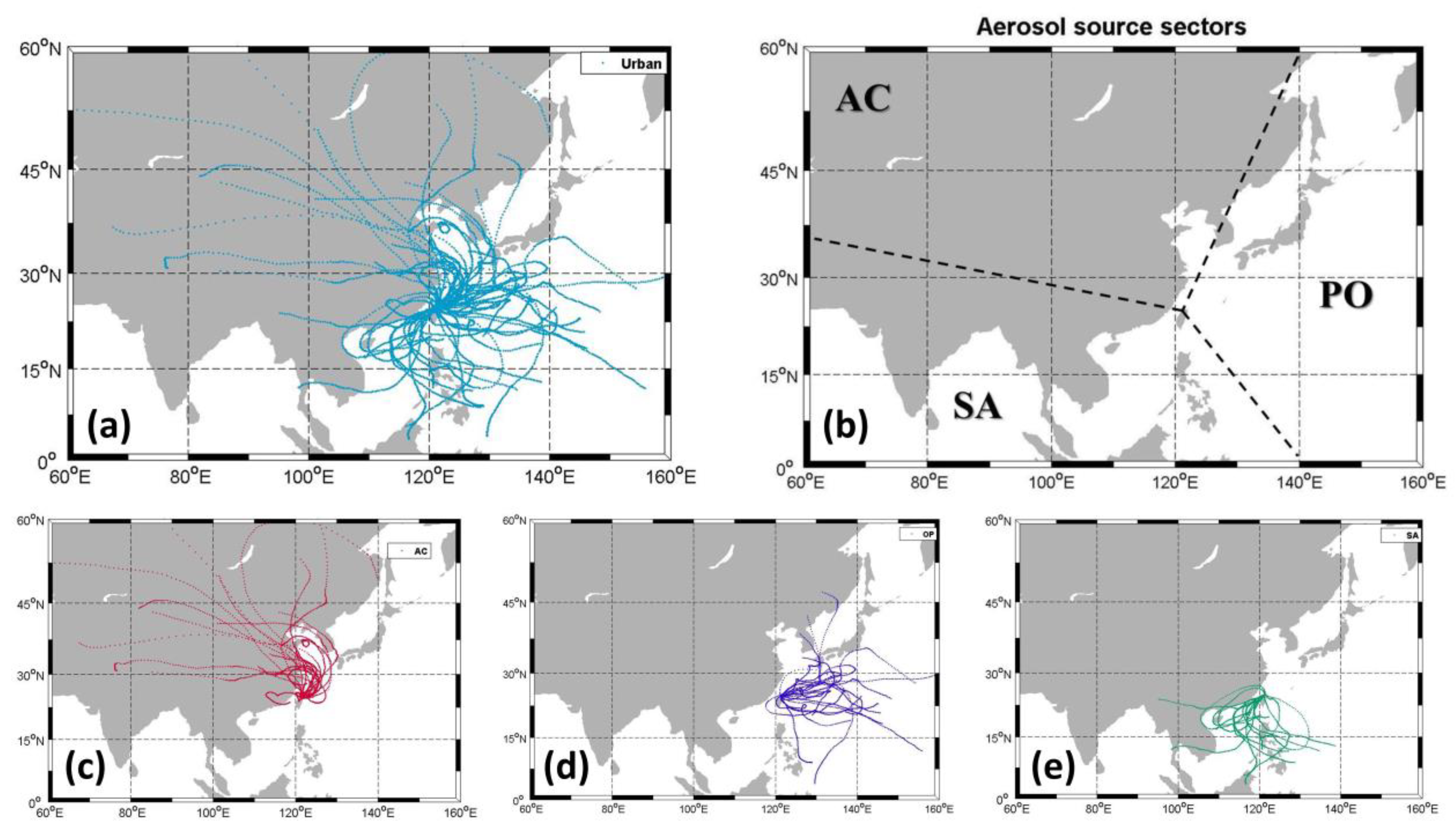
2.3. Source Identification Through Back Trajectory Analysis

In order to identify the source origin of aerosol transport, 5-day back trajectory calculations were carried out using the Hybrid Single-Particle Lagrangian Integrated Trajectory Version 4 (HYSPLIT; Draxler and Rolph, 2003) model. HYSPLIT is an air parcel trajectory and dispersion model maintained by the National Oceanic and Atmospheric Administration (NOAA) Air Resources Laboratory and this model uses wind fields to trace air parcel transport through the atmosphere ([65,66]). In its backward mode, HYSPLIT integrates back in time the path of travel of an air parcel arriving at a receptor location defined by horizontal and vertical coordinates at a given time. Meteorological input data for the back-trajectory calculation were from the NCEP Global Data Assimilation System (GDAS) at 1° × 1° resolution.

3. Results

3.1. Long-Term Data Analysis of Aerosol Optical Properties

The long-term optical properties of aerosols at NCU station (EPA-NCU as the official name shown in AERONET and MPLNET) are shown in Figure 1. Figure 1a shows the monthly variations in AOD at 500 nm (τ500). The observed annual average τ500 was 0.41 ± 0.25 (range of 0.2–1). High values (greater than annual average) of τ500 were observed from February to May, and low values (less than or equal to annual average) during the remaining months. The standard deviation of τ500 was about 0.2 to 0.3, indicating a clue on the high variability of columnar aerosol loading. High τ500 values were found to be similar to the nearby AERONET station (i.e., Taipei_CWB; 25°N, 121°E; 26 m a.s.l.; ≈25 km northeast of EPA-NCU site) in Taipei city, and low values of τ500 were similar to a high-altitude background AERONET site at mountain Lulin (23.51°N, 120.92°E; 2862 m a.s.l.; ≈100 km southeast of EPA-NCU) in central Taiwan. This indicates relatively higher aerosol loading over the study region and made it a complex aerosol environment. The monthly mean τ500 was the highest in March (0.72 ± 0.28), followed by April (0.58 ± 0.22). This was mainly due to the long-range transport of biomass-burning from Indochina region and dust aerosols from arid region in China [23]. It was further confirmed that the EPA-NCU stations have frequent long-range transport events, and to strengthen the transport mechanism, the vertical profiles of aerosol extinction coefficient and trajectories for origin of aerosols were analyzed.
The long-term analysis of the angstrom exponent between 440 nm and 870 nm (α440/870), which stands for aerosol particle sizes (higher value for smaller particle and vice versa), has been plotted in Figure 1b. Annual average of α440/870 was 1.26 ± 0.11 (ranged from 1.34 to 1.05). The maximum value ≈1.4 was found in February followed by the low in April (1.12 ± 0.32), and the minimum was found in September (1.05 ± 0.42). The smallest size of particle observed in February and March is due to the long-rang transported biomass-burning aerosols in the free atmosphere ([67]). Higher values of τ500 in April with lower values of α440/870 indicated the presence of dust aerosols due to Asian dust transport from the Gobi Desert.
Figure 1c shows the monthly Sp averaged from MPLNET data set during 2005–2012. The annual average Sp was 47 ± 21 sr. Sp was the highest in March (54 ± 23 sr), followed by 51 ± 23 sr in April, and the lowest value was observed during May (37 ± 17 sr). As aforementioned, the Sp is mainly dependent on aerosol physicochemical properties and can be further interpreted to aerosol types.

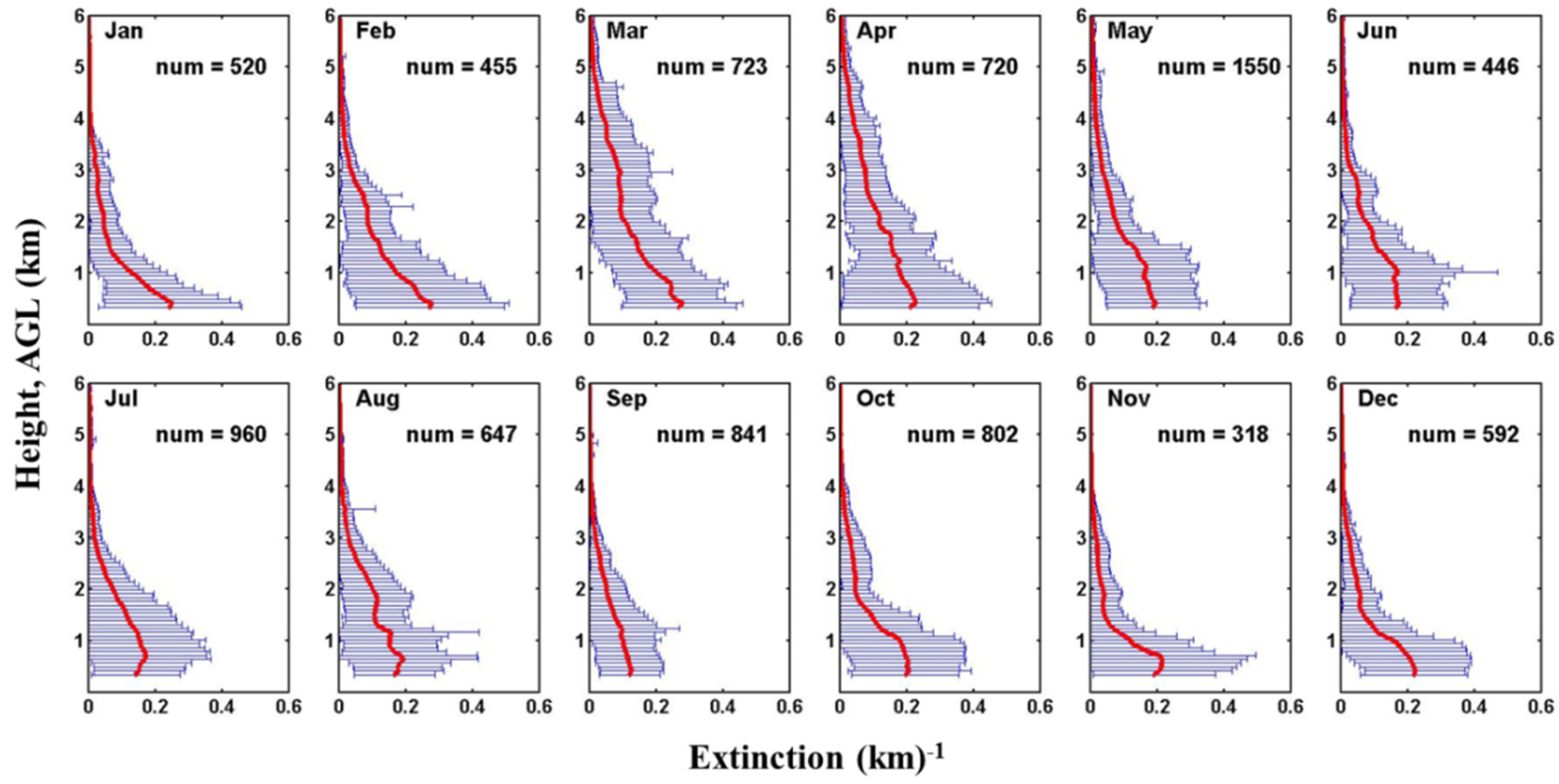
3.2. Monthly Aerosol Extinction Profiles

Figure 2 shows the vertical profile of aerosol extinction coefficient for each month averaged for the period of 2005–2012. As is clearly seen in Figure 3, the extinction coefficient extended from the surface to ≈6 km during March, April, and May, whereas the extinction coefficient was almost zero at ≈4 km during other months. A small aerosol layer at 2–4 km was observed over the region during March. This type of aerosol layer is mainly attributed to the dry convicting lift of air pollutants from far-off regions and subsequent horizontal transport of aerosols ([23,68]). On average, the vertical aerosol distribution follows the scale height, higher aerosol extinction near the surface and decreases as height increases.

3.3. Aerosol Vertical Distribution, Source Region, and Optical Properties

According to the discussion in Section 3.2, the air masses in the PBL and free atmosphere could be from different source origins and imply different aerosol types. In order to clearly define the impacts of vertical distribution on the optical properties (i.e., τ500, α440/870, and Sp), we divided the classification of vertical distribution into two categories based on [23], i.e., single-layer (type 1) and two-layer (type 2) aerosol structures of the aerosol extinction coefficient.

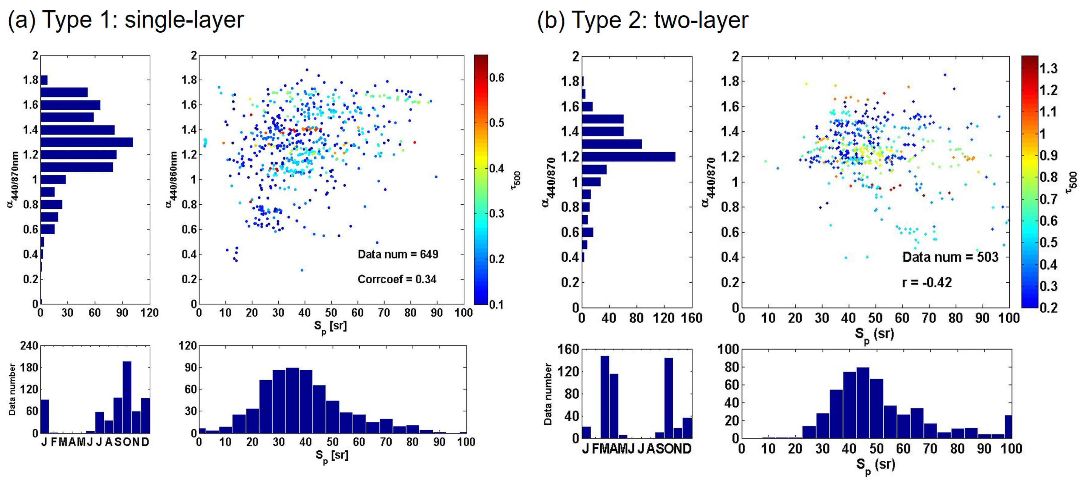
3.3.1. Characteristics of Single-Layer Aerosol Structure

The averaged aerosol extinction along with one standard deviation for single aerosol layer structure (type 1) is shown in Figure 3a. The aerosols are concentrated in the lower troposphere within 2 km altitude and the averaged extinction coefficient value is less than 0.2 km−1 at the near surface. This confinement of aerosols was attributed to boundary layer dynamics and inversion layer below free atmosphere. The total number of days corresponding to type 1 was 55 days (total number of data points = 649) and there were a maximum of 15 days in October, followed by a total of 11 days in September (Figure 4c). The single-layered structure of aerosols mainly occurred in the autumn and winter, especially in September and October, as shown in Figure 3c.
In order to explore the possible sources and types of aerosols, the backward trajectory simulations were employed. Five-day back trajectories (Figure 4a) made at a height of 500 m represent the occurrence height of maximum aerosol extinction. The back trajectories for type 1 showed disorder and originated from all the directions. We further divided the total area into three regions (Figure 4b), viz., the Asia continental region (AC; Mongolia, Tibet, Xinjiang, North China and Central China region, Japan, and South Korea), the Pacific Ocean region (PO; Northwestern Pacific), and the Southeast Asia region (SA; Southeast Asia and southern China). Back trajectory analysis showed that a total of 28 day (number of data points = 458), 12 day (number of data points = 59), and 21 day (number of data points = 154) air masses were coming from AC, PO, and SA regions to EPA-NCU site, respectively (Figure 4c,e). It is important to note that few trajectories passed through more than one region, which resulted in double counting of data numbers in Table 1.
Combining information of α440/870 and Sp can help us to distinguish the aerosol types. Figure 5a shows the scatter plot of α440/870 and Sp with code denoting τ500 together with the histograms representing spread of samples and color magnitude of for type 1. The τ values were in the range of 0.1 to 0.6, with an average value of 0.21; α440/870 was between 0.6 and 1.8, with an average value of 1.26 ± 0.31. The Sp is concentrated between 30 and 60 sr with an average of 39 sr. Previous studies reported that the Sp values of (37 ± 9) sr and (33 ± 6) sr were for dust and marine aerosols, respectively [69].
Table 1 presents the aerosol optical properties of type 1, and for the values in different source sectors. The τ500, α440/870, and Sp for AC region were 0.24 ± 0.11, 1.34 ± 0.19, and (39 ± 16) sr, respectively. The real part (nr = 1.45) of the refractive index was small and relatively close to the urban aerosol refractive index (nr = 1.46). The τ500, α440/870, and Sp for PO source region were 0.19 ± 0.1, 1.24 ± 0.31, and (30 ± 12) sr, respectively. The moderate high value of α440/870 suggests that the mixture of coarse mode sea salt aerosol and fine mode urban aerosol. The similar value of Sp about 33 ± 6 sr was also reported by [28] in the Indian Ocean. For the SA region, the average τ500 and α440/870 were 0.19 ± 0.08 and 1.32 ± 0.32, respectively, indicating the abundant fine mode particle aerosol compared to other source regions. The average of Sp was 38 ± 17 sr in the SA region; however, the data histogram (not shown) exhibited two distinguished peaks: the first peak ranged between 20 and 40 sr, whereas the second peak ranged between 45 and 60 sr. The median value of the first peak was about 30 sr corresponding to marine type aerosols, while the second peak was similar to the results from local pollutants. The complex of emission sources (i.e., marine, ship, local Taiwan island) in the SA region might need further study in the future when more data becomes available. Regarding to the AERONET derived single-scattering albedo at 440 nm wavelength (ω440) and asymmetry factor at 440 nm wavelength (g440), aerosols from AC and SA regions show similar values and suggest a moderate absorption compared to that from PO regions. The result implies the segment of source sector with backward trajectory may not be sufficient to aerosol classification for majority of data.

3.3.2. Characteristics of Two-Layer Aerosol Structure

Two-layer structured vertical profiles have been classified as type 2 ([23]). In this type, we found another peak with an aerosol extinction coefficient at 2–4 km in addition to the extinction coefficient peak that appears at the near surface. Lower than 2 km, the aerosol vertical profile has a similar impact as type 1, but at the 2–4 km range, the average extinction coefficient is 0.25 km−1 in type 2, whereas it is only less than 0.1 km−1 in type 1. The two-layered structure mainly occurs in spring and winter seasons, and a few days in other months, as shown in Figure 3d.
The τ500, α440/870, and Sp for all observations (total number of data points = 503) under the spread and histograms for two-layer aerosol structure (type 2) are shown in Figure 5b. From the Figure 5b it can be observed that τ500 is between 0.1 and 1.5, with an average of 0.51 ± 0.26; α440/870 is between 0.34 and 1.85, with an average of 1.23 ± 0.26; and Sp ranges between 30 and 80 sr with an average of 52 ± 23 sr.
These two-layered aerosol structures high-up and low-down are caused by the different delivery mechanisms; therefore, they can be tracked by the use of air mass back trajectories analysis in the HYSPLIT model (e.g., [23]). In addition, according to a database (https://airtw.epa.gov.tw/CHT/Forecast/Sand.aspx) provided by the Taiwan Environmental Protection Agency (EPA) which determines the date for a sandstorm event, we can classify dust transport as taking place down low. The dust and biomass-burning cases for two-layer aerosol structure are defined as follows:
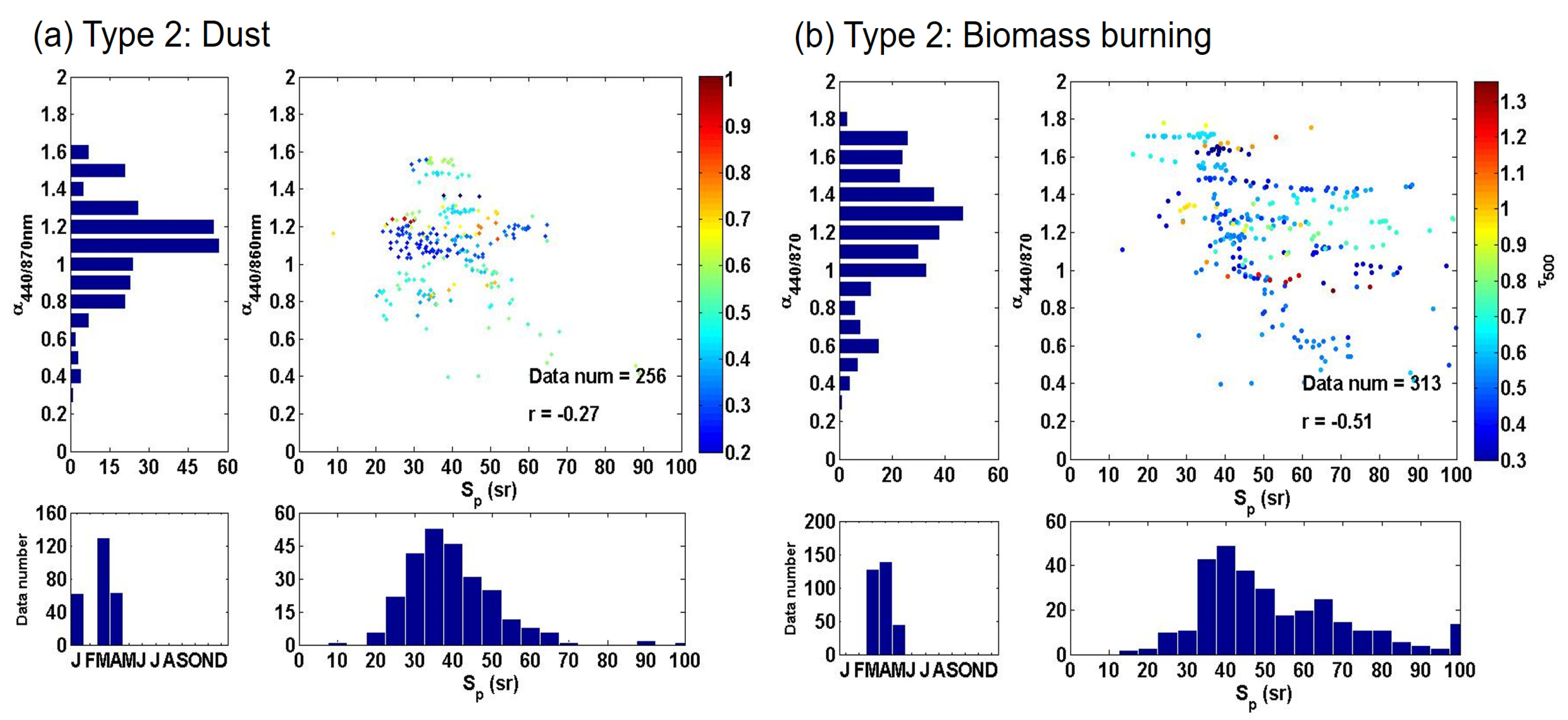
  • Two-layer aerosol structure (dust case): Sandstorm pollution recorded by the EPA on the same day and the main source of air mass from the AC region (mainly from the elevated regions over northern China and Mongolia and covered the longest distance along China’s coast). Those mineral dust particles usually transport near the surface behind of a frontal system, and occasionally intrude to higher levels via frontal dynamics.
  • Two-layer aerosol structure (biomass-burning case): Transport of springtime biomass-burning emissions from the source regions over SA (comprising Cambodia, Laos, Myanmar, and Thailand). Those aerosols mainly transport in free atmosphere and arrive in Taiwan at higher elevation.

3.4. Dust Case

From the vertical profile of the aerosol extinction coefficient, it can be seen that dust mainly transports in the height region of 500–2000 m (Figure 6a). We carefully checked the airflow source with backward trajectories; it was found that low in the atmosphere (500 m), the aerosol sources were from the northern desert regions of China. In addition, we also found that three dust events (on 18 March, 28 March, and 25 November in 2005) had influences on biomass-burning transport from Indochina through the backward trajectory analysis at 2500 m. A recent publication by [70] also demonstrated a long-range transport event with concurrent dust and biomass-burning aerosol layers based on EPA-NCU lidar observation. More study related to the coexisting of dust and biomass-burning over the west Pacific can be explored in the future.
The τ500 for the dust events over the years was at about 0.45 ± 0.16 with the averaged α440/870 of about 1.10 ± 0.24. Coarse particle size was higher when compared to other regions, and Sp was found in the range of 20 to 60 sr with an average of 40 ± 16 sr (Figure 7a), and followed the normal Gaussian distribution with the median value of 40 sr. The estimation Sp of dust aerosols in African region was 37 ± 9 sr, and it also found that it changed in the course of dust transportation when mixed with urban pollutants ([71]).

3.5. Biomass-Burning Case

The vertical distribution of aerosol extinction coefficient shows a significant secondary peak 0.1 km−1 in the height range of 3–4 km approximately (Figure 6b). Based on the back trajectory at the height of 3000 m above sea level, we found that the air mass sources were from the SA region (taken over 22 days; total number of data points = 313). The analyzed averaged optical characteristics for biomass-burning were τ500 of 0.58 ± 0.20, α440/870 of 1.22 ± 0.33, and Sp of 53 ± 21 sr (Table 2). The distribution of Sp shows double peaks, the first peak in the range of 20 to 50 sr and the second peak in the range of 60 to 70 sr (Figure 7b). Compared to the mean Sp value of 47 ± 21 sr in northern Taiwan, it was found that the first peak could be linked to mixture of anthropogenic and biomass-burning aerosols. When the air by the burning of biomass and other outside influences affects the area, it gives rise in Sp to a more apparent second peak (60 to 70 sr) due to high absorption of light by the high altitude aerosols. The similar value of Sp as 63 ± 10 sr for African savannah biomass-burning was also reported by [17].

4. Discussion

In this section, we further discuss the Sp of urban, dust, and biomass-burning aerosols representing the subtropical region of East Asia based on aforementioned analysis with additional estimations. In the previous section, based on statistics of long-term (2005–2012) EPA-NCU MPL dataset, we found that the average value of Sp is 47 ± 21 sr. The results report a mixture of dust and biomass-burning aerosols. In order to quantify the Sp value of urban aerosols, we selected cases with two constraints: (1) type 1 vertical profile and only from AC source region, (2) no dust events. We estimated the mean Sp of urban aerosols to be 42 ± 18 sr, which is in agreement with the value of 45 ± 10 suggested by [19] (see Table 3). For oceanic aerosols, we suggested that the Sp value can be estimated from PO source region in type 1, which is 30 ± 12 sr. This value is very similar to the values (32–33) provided by [72]. It should be noted that a higher value observed in our study may have been due to the mixing of local urban aerosols during the transport to northern Taiwan.
Regarding dust aerosol, we selected cases that met the criteria of type 1 classification and EPA dust event dates. Only one dust event was recorded on 29 January 2007, and comprises 37 profiles. As shown in Figure 8a, the dust plume was transported near the surface and constrained within 1.4 km height. The maximum aerosol extinction coefficient was 0.2 ± 0.04 km−1 observed at 1 km. Figure 8b shows the scattering plot of Sp and α440/870 for all type 1 data points, in which red dots highlight the dust signature. The α440/870 was about 1.05, suggesting a slightly coarser particle for transported dust when compared to the mean α440/870 value of 1.29 for type 1 at EPA-NCU station. The number distribution of Sp for dust data is shown in Figure 8c. The Sp ranged between 25 and 50 sr with an average of 34 ± 6 sr. The value shows good agreement with previous studies ([71,73]) that measured dust particles (Table 3). It is worth mentioning that a large portion of dust events may have a mixture of anthropogenic aerosols during the transport. Those mixed events can have a higher lidar ratio of up to 40 sr, as described in dust cases of type 2 profile.
The transport of biomass-burning aerosols to Taiwan is often characterized by upper-level transport, which makes it difficult to separate the biomass-burning Sp value from the total columnar mean Sp value (as obtained from the EPA-NCU MPLNET). The histogram of Sp number distribution for biomass-burning cases in type 2 shows a bimodal distribution (Figure 7b), where the first peak ranged from 30 to 50 sr and the second peak ranged from 60 to 80 sr. In type 2, the aerosol type contributing to the surface layer can be urban, oceanic, or dust, whereas biomass-burning aerosols are attributed to the upper level. Large portions of aerosols are suspended within the surface layer. As listed in Table 3, the mean Sp values for urban, oceanic, and dust are between 30–42 sr, and correspond to the first peak of Figure 7b. That suggests the domination of surface layer transport. In other words, the second peak of Figure 7b may represent the domination of upper-level transport, which is mainly attributed to biomass-burning aerosols. The mode Sp of the second peak was 69 ± 12 sr, representing biomass-burning aerosols originating from Indochina. Our result shows a little higher value compared to the literature value of 63 ± 10 sr for African biomass-burning ([17]).

5. Conclusions

Lidar ratio (Sp) is a distinctive aerosol optical property and can be used for aerosol type classification, which is important for pollution source identification and radiative forcing assessment. This study analysed the long-term (2005–2012) observations of MPLNET and AERONET from a rural site (EPA-NCU) in northern Taiwan located in the western North Pacific. Those observations, consisting of aerosol optical characteristics, extinction coefficient profiles, and lidar ratios, in conjunction with air mass trajectories, were further used to investigate the relationship between aerosol types and aerosol optical properties over the region. The important findings are as follows:
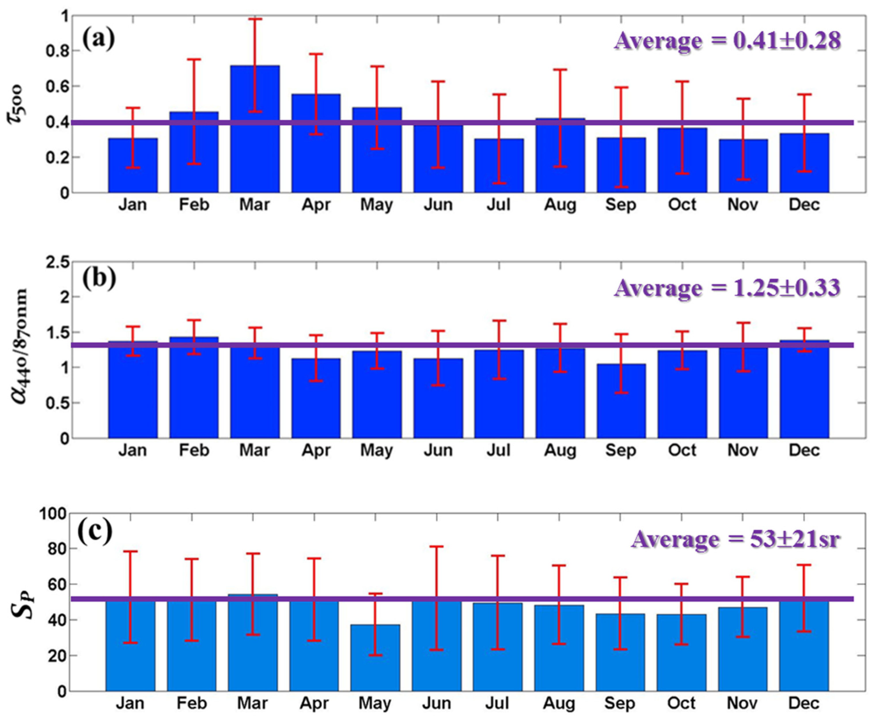
  • The long-term average values of τ500, α440/870, and Sp were found to be 0.41 ± 0.28, 1.25 ± 0.33, and (47 ± 21) sr, respectively.
  • The highest τ500 (0.72 ± 0.28) and Sp (54 ± 23 sr) values in the month of March were primarily attributed to the long-range transport of biomass-burning aerosols from Indochina.
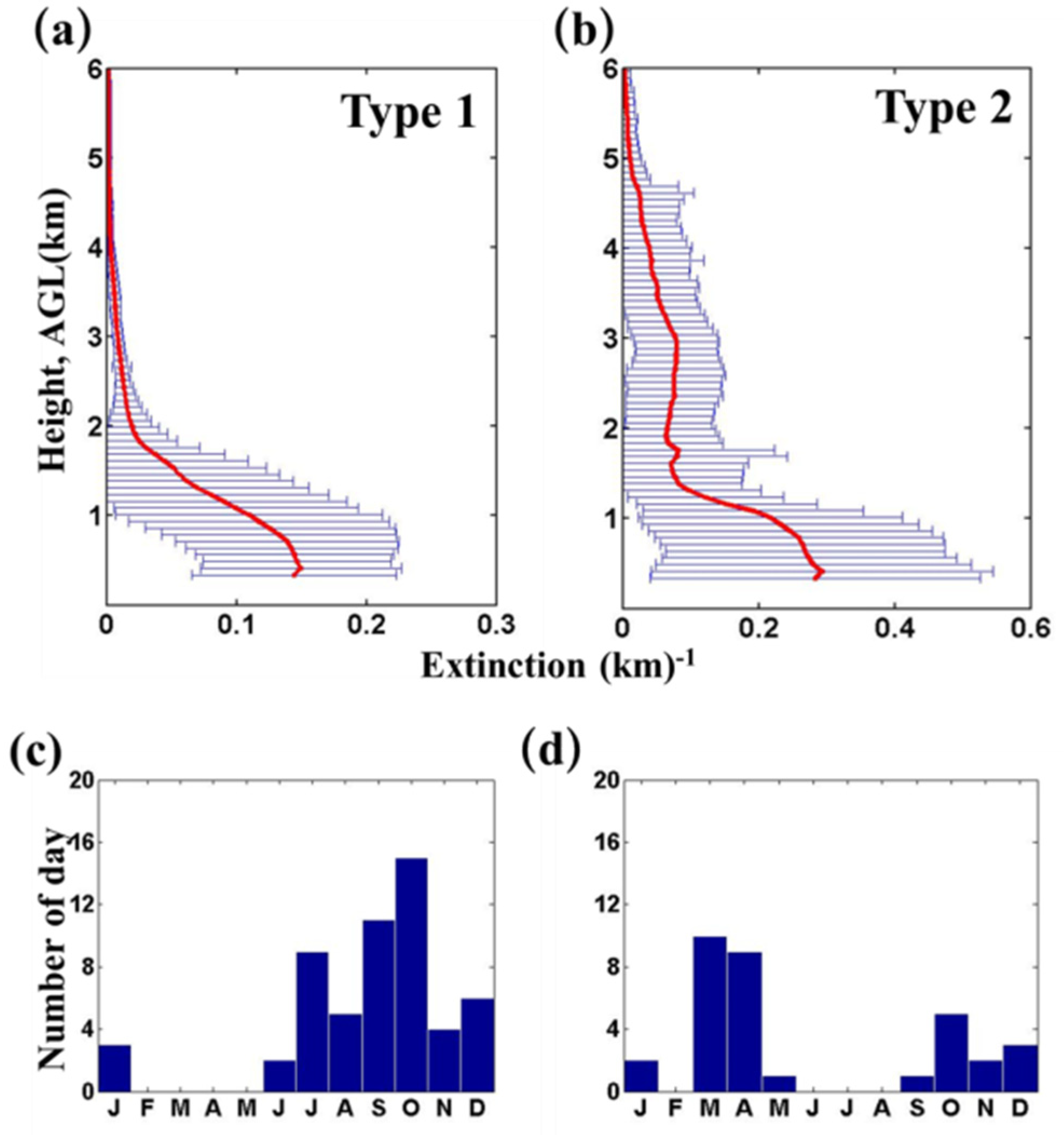
  • Two types of aerosol structure were classified based on the vertical cross-sections of aerosols. Type 1 aerosol structure (near-surface aerosol transport mainly prevails during October–November) showed low values τ500 and Sp and mainly originated from the AC region (τ500: 0.24 ± 0.11; Sp: 39 ± 8 sr), PO region (0.19 ± 0.10; 30 ± 12 sr), and SA region (0.19 ± 0.11; 38 ± 17 sr).
  • Type 2 aerosol transport (mainly during March–April at an altitude of 3 to 6 km) was associated with high τ500 (0.51 ± 0.22), α440/870 (1.23 ± 0.26), and Sp (52 ± 23 sr).
  • For type 2 dust case, the estimated τ500, α440/870, and Sp were found to be 0.45 ± 0.16, 1.10 ± 0.24, and (40 ± 16) sr, respectively. For type 2 biomass-burning case, the estimated τ500, α440/870, and Sp were found to be 0.58 ± 0.20, 1.22 ± 0.33, and (53 ± 21) sr, respectively.
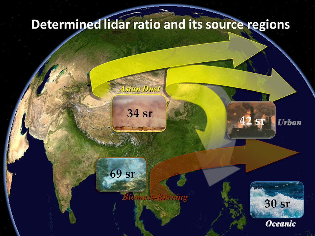
  • Sp values, for four major aerosol types over northern Taiwan, were estimated to be 42 ± 18 sr (urban), 34 ± 6 sr (dust), 69 ± 12 sr (biomass-burning), and 30 ± 12 sr (oceanic).
The findings of this study offer a reference for future attempts to monitor the sources of aerosol over Taiwan and western North Pacific. Results of Sp value provide useful references for aerosol classification and air pollution identification in this region. This kind of study is also important for resolving aerosol-perturbed atmospheric circulation (e.g., [74,75,76]) and temporal changes in regional air quality (e.g., [77,78]). Nevertheless, due to the principle of Mie elastic lidar, the Sp value only represents a columnar integrated number by using a retrieval method. The newly available lidar ratio datasets with data fusion technology, such as AERONET version 3 product (e.g., [34,79]), MPLNET version 3 depolarization ratio product, Raman lidar ([72]), and high spectral resolution lidar (e.g., [42,43,44,45]) do also give an aspect of aerosol classification. More observation and data analyses are needed to further explore the relationship between aerosol types and aerosol optical properties over the region.

Author Contributions

Conceptualization, S.-H.W.; methodology, H.-W.L., H.-Y.H., and Y.-C.W.; writing—original draft preparation, S.-H.W.; writing—review and editing, S.K.P.; project administration, N.-H.L. and E.J.W.; funding acquisition, S.-C.C. All authors have read and agreed to the published version of the manuscript.

Funding

This work is funded by the Taiwan Environmental Protection Administration under grant EPA-107-FA11-03-A071 and by the Ministry of Science and Technology under grant 108-2111-M-008-025.

Acknowledgments

The NASA MPLNET and AERONET are funded by the NASA Earth Observing System and Radiation Sciences Program. The authors gratefully acknowledge the NOAA Air Resources Laboratory for the provision of the HYSPLIT transport and dispersion model used in this publication. We are also grateful to the National Center for High-performance Computing for computer time and facilities.

Conflicts of Interest

The authors declare no conflict of interest.

References

  1. Charlson, R.J.; Schwartz, S.E.; Hales, J.M.; Cess, R.D.; Coakley, J.D.; Hansen, J.E.; Hofmann, D.J. Climate forcing by anthropogenic aerosols. Science 1992, 255, 423–430. [Google Scholar] [CrossRef] [PubMed]
  2. Penner, J.E.; Charlson, R.J.; Hales, J.M.; Laulainen, N.S.; Leifer, R.; Novakov, T.; Ogren, J.; Radke, L.F.; Schwartz, S.E.; Travis, L. Quantifying and minimizing uncertainty of climate forcing by anthropogenic aerosols. Bull. Am. Meteorol. Soc. 1994, 75, 375–400. [Google Scholar] [CrossRef]
  3. Intergovernmental Panel on Climate Change. Climate Change 2007, Working Group I Report—The Physical Science Basis; Solomon, S., Qin, D., Manning, M., Marquis, M., Averyt, K., Tignor, M.M.B., LeRoy Miller, H., Jr., Chen, Z., Eds.; Cambridge University Press: New York, NY, USA, 2007. [Google Scholar]
  4. Kaufman, Y.J.; Tanre, D.; Gordon, H.R.; Nakajima, T.; Lenoble, J.; Frouin, R.; Grassl, H.; Hermann, B.M.; King, M.D.; Teillet, P.M. Passive Remote Sensing of Tropospheric Aerosol and Atmospheric Correction for the Aerosol Effect. J. Geophys. Res. 1997, 102, 16815–16830. [Google Scholar] [CrossRef] [Green Version]
  5. Yu, H.B.; Chin, M.; Winker, D.M.; Omar, A.H.; Liu, C.K.; Diehl, T. Global View of Aerosol Vertical Distributions from CALIPSO Lidar Measurements and GOCART Simulations: Regional and Seasonal Variations. J. Geophys. Res. 2010, 115, D00H30. [Google Scholar] [CrossRef] [Green Version]
  6. Haywood, J.M.; Ramaswamy, V. Global sensitivity studies of the direct radiative forcing due to anthropogenic sulfate and blackcarbon aerosols. J. Geophys. Res. 1998, 103, 6043–6058. [Google Scholar] [CrossRef]
  7. Gadhavi, H.; Jayaraman, A. Airborne lidar study of the vertical distribution of aerosols over Hyderabad, an urban site in central India, and its implication for radiative forcing calculations. Ann. Geophys. 2006, 24, 2461–2470. [Google Scholar] [CrossRef]
  8. Chew, B.N.; Campbell, J.; Hyer, E.J.; Salinas, S.V.; Reid, J.S.; Welton, E.J.; Holben, B.N.; Liew, S.C. Relationship between aerosol optical depth and particulate matter over Singapore: Effects of aerosol vertical distributions. Aerosol Air Qual. Res. 2016, 16, 2818–2830. [Google Scholar] [CrossRef]
  9. Wang, S.-H.; Welton, E.J.; Holben, B.N.; Tsay, S.-C.; Lin, N.-H.; Giles, D.; Stewart, S.A.; Janjai, S.; Nguyen, X.A.; Hsiao, T.-C. Vertical distribution and columnar optical properties of springtime biomass-burning aerosols over Northern Indochina during 2014 7-SEAS campaign. Aerosol Air Qual. Res. 2015, 15, 2037–2050. [Google Scholar] [CrossRef] [Green Version]
  10. Hee, W.S.; San Lim, H.; Jafri, M.Z.M.; Lolli, S.; Ying, K.W. Vertical profiling of aerosol types observed across monsoon seasons with a Raman lidar in Penang Island, Malaysia. Aerosol Air Qual. Res. 2016, 16, 2843–2854. [Google Scholar] [CrossRef] [Green Version]
  11. Muñoz Magnino, R.; Alcafuz, R.I. Variability of urban aerosols over Santiago, Chile: Comparison of surface PM10 concentrations and remote sensing with ceilometer and lidar. Aerosol Air Qual. Res. 2012, 12, 8–19. [Google Scholar] [CrossRef]
  12. Jayaraman, A.; Subbaraya, B.H. In situ measurements of aerosol extinction profiles and their spectral dependencies at tropospheric levels. Tellus 1993, 45B, 473–478. [Google Scholar] [CrossRef]
  13. Ramachandran, S.; Jayaraman, A. Balloon-borne study of the upper tropospheric and stratospheric aerosols over a tropical station in India. Tellus 2003, 55B, 820–836. [Google Scholar] [CrossRef]
  14. He, Q.S.; Li, C.C.; Mao, J.T.; Lau, A.K.H. A study on aerosol extinction-to-backscatter ratio with combination of micro-pulse lidar and MODIS over Hong Kong. Atmos. Chem. Phys. 2006, 6, 3243–3256. [Google Scholar] [CrossRef] [Green Version]
  15. Devara, P.C.S.; Raj, P.E.; Pandithurai, G. Aerosol-profile measurements in the lower troposphere with four-wavelength bistatic argon-ion lidar. Appl. Opt. 1995, 34, 4416–4425. [Google Scholar] [CrossRef]
  16. Parameswaran, K.; Rajan, R.; Vijayakumar, G.; Rajeev, K.; Moorthy, K.K.; Nair, P.R.; Satheesh, S.K. Seasonal and long term variations of aerosol content in the atmospheric mixing region at a tropical station on the Arabian sea-coast. J. Atmos. Sol. Terr. Phys. 1998, 60, 17–25. [Google Scholar] [CrossRef]
  17. Welton, E.J.; Voss, K.J.; Gordon, H.R.; Maring, H.; Smirnov, A.; Holben, B.N.; Schmid, B.; Livingston, J.M.; Russell, P.B.; Durkee, P.A.; et al. Ground-based lidar measurements of aerosols during ACE-2: Lidar description, results, and comparisons with other ground-based and airborne measurements. Tellus 2000, 52B, 636–651. [Google Scholar] [CrossRef] [Green Version]
  18. Chen, W.B.; Kuze, H.; Uchiyama, A.; Suzuki, Y.; Takeuchi, N. One-year observation of urban mixed layer characteristics at Tsukuba, Japan using a micro pulse lidar. Atmos. Environ. 2001, 35, 4273–4280. [Google Scholar] [CrossRef]
  19. Campbell, J.R.; Welton, E.J.; Spinhirne, J.D.; Ji, Q.; Tsay, S.; Piketh, S.J.; Barenbrug, M.; Holben, B.N. Micropulse lidar observations of tropospheric aerosols over northeastern South Africa during the ARREX and SAFARI 2000 dry season experiments. J. Geophys. Res. 2003, 108, 8497. [Google Scholar] [CrossRef]
  20. Schmid, B.; Ferrare, R.; Flynn, C.; Elleman, R.; Covert, D.; Strawa, A.; Welton, E.; Turner, D.; Jonsson, H.; Redemann, J. How well do state-of-the-art techniques measuring the vertical profile of tropospheric aerosol extinction compare? J. Geophys. Res. 2006, 111, D05S07. [Google Scholar] [CrossRef]
  21. Hayasaka, T.; Satake, S.; Shimizu, A.; Sugimoto, N.; Matsui, I.; Aoki, K.; Muraji, Y. Vertical distribution and optical properties of aerosols observed over Japan during the Atmospheric Brown Clouds–East Asia Regional Experiment 2005. J. Geophys. Res. 2007, 112, D22S35. [Google Scholar] [CrossRef]
  22. He, Q.; Li, C.; Mao, J.; Lau, A.K.-H.; Chu, D.A. Analysis of aerosol vertical distribution and variability in Hong Kong. J. Geophys. Res. 2008, 113, D14211. [Google Scholar] [CrossRef]
  23. Wang, S.-H.; Lin, N.-H.; Chou, M.-D.; Tsay, S.-C.; Welton, E.J.; Hsu, N.C.; Giles, D.M.; Liu, G.-R.; Holben, B.N. Profiling transboundary aerosols over Taiwan and assessing their radiative effects. J. Geophys. Res. 2010, 115, D00K731. [Google Scholar] [CrossRef]
  24. Kent, G.S.; Trpte, C.R.; Lucker, P.L. Long-term Stratospheric Aerosol and Gas Experiment I and II measurements of upper tropospheric aerosol extinction. J. Geophys. Res. 1998, 103, 28863–28874. [Google Scholar] [CrossRef]
  25. Spinhirne, J.D.; Palm, S.P.; Hart, W.D.; Hlavka, D.L.; Welton, E.J. Cloud and aerosol measurements from GLAS: Overview and initial results. Geophys. Res. Lett. 2005, 32, L22S03. [Google Scholar] [CrossRef]
  26. Mamouri, R.-E.; Ansmann, A. Potential of polarization lidar to provide profiles of CCN- and INP-relevant aerosol parameters. Atmos. Chem. Phys. 2016, 16, 5905–5931. [Google Scholar]
  27. Sassen, K.; Cho, B.S. Subvisual-Thin Cirrus LIDAR Dataset for Satellite Verification and Climatological Research. J. Appl. Meteorol. 1992, 31, 1275–1285. [Google Scholar] [CrossRef] [Green Version]
  28. Welton, E.J.; Voss, K.J.; Flatau, P.J.; Markowicz, K.; Campbell, J.R.; Spinhirne, J.D.; Gordon, H.R.; Johnson, J.E. Measurements of aerosol vertical profiles and optical properties during INDOEX 1999 using micropulse lidars. J. Geophys. Res. 2002, 107, 8019. [Google Scholar] [CrossRef]
  29. Pelon, J.; Flamant, C.; Chazette, P.; Leon, J.-F.; Tanre, D.; Sicard, M.; Satheesh, S.K. Characterization of aerosol spatial distribution and optical properties over the Indian Ocean from airborne LIDAR and radiometry during INDOEX’99. J. Geophys. Res. 2002, 107, 8029. [Google Scholar] [CrossRef] [Green Version]
  30. McGill, M.J.; Hlavka, D.L.; Hart, W.D.; Welton, E.J.; Campbell, J.R. Airborne lidar measurements of aerosol optical properties during SAFARI-2000. J. Geophys. Res. 2003, 108, 8493. [Google Scholar] [CrossRef]
  31. Flamant, C.; Pelon, J.; Chazette, P.; Trouillet, V.; Quinn, P.K.; Frouin, R.; Bruneau, D.; Leon, J.-F.; Bates, T.; Johnson, J.; et al. Airborne lidar measurements of aerosol spatial distribution and optical properties over the Atlantic Ocean during an European pollution outbreak of ACE-2. Tellus 2000, 52B, 662–677. [Google Scholar] [CrossRef] [Green Version]
  32. Tsay, S.C.; Hsu, N.C.; Lau, W.K.M.; Li, C.; Gabriel, P.M.; Ji, Q.; Holben, B.N.; Judd Welton, E.; Nguyen, A.X.; Janjai, S.; et al. From BASE-ASIA toward 7-SEAS: A satellite-surface perspective of boreal spring biomass-burning aerosols and clouds in Southeast Asia. Atmos. Environ. 2013, 78, 20–34. [Google Scholar] [CrossRef] [Green Version]
  33. Wang, S.-H.; Tsay, S.-C.; Lin, N.-H.; Chang, S.-C.; Li, C.; Welton, E.J.; Holben, B.N.; Hsu, N.C.; Lau, K.-M.; Lolli, S.; et al. Origin, transport, and vertical distribution of atmospheric pollutants over the northern South China Sea during 7-SEAS/Dongsha experiment. Atmos. Environ. 2013, 78, 124–133. [Google Scholar] [CrossRef]
  34. Shin, S.-K.; Tesche, M.; Noh, Y.; Müller, D. Aerosol-type classification based on AERONET version 3 products. Atmos. Meas. Tech. 2019, 12, 3789–3803. [Google Scholar] [CrossRef] [Green Version]
  35. Siomos, N.; Fountoulakis, I.; Natsis, A.; Drosoglou, T.; Bais, A. Automated Aerosol Classification from Spectral UV Measurements Using Machine Learning Clustering. Remote Sens. 2020, 12, 965. [Google Scholar] [CrossRef] [Green Version]
  36. Chen, Q.-X.; Huang, C.-L.; Yuan, Y.; Mao, Q.-J.; Tan, H.-P. Spatiotemporal Distribution of Major Aerosol Types over China Based on MODIS Products between 2008 and 2017. Atmosphere 2020, 11, 703. [Google Scholar] [CrossRef]
  37. Nicolae, D.; Vasilescu, J.; Talianu, C.; Binietoglou, I.; Nicolae, V.; Andrei, S.; Antonescu, B. A neural network aerosol-typing algorithm based on lidar data. Atmos. Chem. Phys. 2018, 18, 14511–14537. [Google Scholar] [CrossRef] [Green Version]
  38. Ansmann, A.; Seifert, P.; Tesche, M.; Wandinger, U. Profiling of fine and coarse particle mass: Case studies of Saharan dust and Eyjafjallajökull/Grimsvötn volcanic plumes. Atmos. Chem. Phys. 2012, 12, 9399–9415. [Google Scholar] [CrossRef] [Green Version]
  39. Kim, M.-H.; Omar, A.H.; Tackett, J.L.; Vaughan, M.A.; Winker, D.M.; Trepte, C.R.; Hu, Y.; Liu, Z.; Poole, L.R.; Pitts, M.C.; et al. The CALIPSO version 4 automated aerosol classification and lidar ratio selection algorithm. Atmos. Meas. Tech. 2018, 11, 6107–6135. [Google Scholar] [CrossRef] [Green Version]
  40. Georgoulias, A.K.; Marinou, E.; Tsekeri, A.; Proestakis, E.; Akritidis, D.; Alexandri, G.; Zanis, P.; Balis, D.; Marenco, F.; Tesche, M.; et al. A first case study of CCN concentrations from spaceborne lidar observations. Remote Sens. 2020, 12, 1557. [Google Scholar] [CrossRef]
  41. Ackermann, J. The extinction-to-backscattering ratio oftropospheric aerosol: A numerical study. J. Atmos. Ocean. Technol. 1998, 15, 1043–1050. [Google Scholar] [CrossRef]
  42. Perez-Ramirez, D.; Whiteman, D.N.; Veselovskii, I.; Colarco, P.; Korenski, M.; da Silva, A. Retrievals of aerosol single scattering albedo by multiwavelength lidar measurements: Evaluations with NASA Langley HSRL-2 during discover-AQ field campaigns. Remote Sens. Environ. 2019, 222, 144–164. [Google Scholar] [CrossRef] [Green Version]
  43. Burton, S.P.; Ferrare, R.A.; Hostetler, C.A.; Hair, J.W.; Rogeres, R.R.; Obland, M.D.; Obland, M.D.; Butler, C.F.; Cook, A.L.; Harper, D.B.; et al. Aerosol classification using airborne High Spectral Resolution Lidar measurements—Methodology and examples. Atmos. Meas. Tech. 2012, 5, 73–98. [Google Scholar] [CrossRef] [Green Version]
  44. Burton, S.P.; Ferrare, R.A.; Vaughan, M.A.; Omar, A.H.; Rogers, R.R.; Hostetler, C.; Hair, J.W. Aerosol classification from airborne HSRL and comparisons with the CALIPSO vertical feature mask. Atmos. Meas. Tech. 2013, 6, 1397–1412. [Google Scholar] [CrossRef] [Green Version]
  45. Burton, S.P.; Vaughan, M.A.; Ferrare, R.A.; Hostetler, C.A. Separating mixtures of aerosol types in airborne High Spectral Resolution Lidar data. Atmos. Meas. Tech. 2014, 7, 419–436. [Google Scholar] [CrossRef] [Green Version]
  46. Streets, D.G.; Bond, T.C.; Carmichael, G.R.; Fernandes, S.D.; Fu, Q.; He, D.; Klimont, Z.; Nelson, S.M.; Tsai, N.Y.; Wang, M.Q.; et al. An inventory of gaseous and 10 primary aerosol emissions in Asia in the year 2000. J. Geophys. Res. 2003, 108, 8809. [Google Scholar] [CrossRef]
  47. Wenig, M.; Spichtinger, N.; Stohl, A.; Held, G.; Beirle, S.; Wagner, T.; Jahne, B.; Platt, U. Intercontinental transport of nitrogen oxide pollution plumes. Atmos. Chem. Phys. 2003, 3, 387–393. [Google Scholar] [CrossRef] [Green Version]
  48. Chiang, C.-W.; Das, S.K.; Nee, J.-B. An iterative calculation to derive extinction-to-backscatter ratio based on lidar measurements. J. Quant. Spectrosc. Radiat. Transf. 2008, 109, 1187–1193. [Google Scholar] [CrossRef]
  49. Lin, N.-H.; Tsay, S.C.; Maring, H.B.; Yen, M.C.; Sheu, G.R.; Wang, S.H.; Chi, K.H.; Chuang, M.T.; Ou-Yang, C.F.; Fu, J.S.; et al. An overview of regional experiments on biomass burning aerosols and related pollutants in Southeast Asia: From BASE-ASIA and the Dongsha Experiment to 7-SEAS. Atmos. Environ. 2013, 78, 1–19. [Google Scholar] [CrossRef] [Green Version]
  50. Chen, W.-N.; Tsao, C.C.; Nee, J.B. Tropospheric and Lower Stratospheric Temperature Measurement by Rayleigh Lidar. J. Atmos. Sol. -Terr. Phys. 2004, 66, 39–49. [Google Scholar] [CrossRef]
  51. Chen, W.-N.; Tsai, F.-J.; Chou, C.C.-K.; Chang, S.-Y.; Chen, I.-W.; Chen, J.-P. Cases studies of Asian Dust in the Free Atmosphere by Raman Depolarization Lidar at Taipei, Taiwan. Atmos. Environ. 2007, 41, 7698–7714. [Google Scholar] [CrossRef]
  52. Chen, W.-N.; Tsai, F.-J.; Chou, C.C.-K.; Chang, S.-Y.; Chen, Y.-W.; Chen, J.-P. Cases Study of Relationship Between Water-soluble Ca2+ and Lidar Depolarization Ratio for Spring Aerosol in the Boundary Layer. Atmos. Environ. 2007, 41, 1440–1455. [Google Scholar]
  53. Chen, W.-N.; Chen, Y.-W.; Chou, C.C.-K.; Chang, S.-Y.; Lin, P.-H.; Chen, J.-P. Columnar optical properties of tropospheric aerosol by combined lidar and sunphotometer measurements at Taipei, Taiwan. Atmos. Environ. 2009, 43, 2700–2716. [Google Scholar] [CrossRef]
  54. Tsai, J.-H.; Hsu, Y.-C.; Yang, J.-Y. The relationship between volatile organic profiles and emission sources in ozone episode region, a case study in southern Taiwan. Sci. Total Environ. 2004, 328, 131–142. [Google Scholar] [CrossRef] [PubMed]
  55. Omar, A.H.; Winker, D.M.; Vaughan, M.A.; Hu, Y.; Trepte, C.R.; Ferrare, R.A.; Lee, K.-P.; Hostetler, C.A.; Kittaka, C.; Rogers, R.R.; et al. The CALIPSO Automated Aerosol Classification and Lidar Ratio Selection Algorithm. J. Atmos. Ocean. Technol. 2009, 26, 23–32. [Google Scholar] [CrossRef]
  56. Liu, C.-M.; Young, C.-Y.; Lee, Y.-C. Influence of Asian Dust Storms on Air Quality in Taiwan. Sci. Total. Environ. 2006, 368, 884–897. [Google Scholar] [CrossRef] [PubMed]
  57. Chuang, M.-T.; Chou, C.-C.-K.; Lin, N.-H.; Takami, A.; Hsiao, T.-C.; Lin, T.-H.; Fu, J.-S.; Pani, S.K.; Lu, Y.R.; Yang, T.Y. A simulation study on PM2.5 sources and meteorological characteristics at the northern tip of Taiwan in the early stage of the Asian haze period. Aerosol Air Qual. Res. 2017, 17, 3166–3178. [Google Scholar] [CrossRef] [Green Version]
  58. Pani, S.K.; Ou-Yang, C.F.; Wang, S.H.; Ogren, J.A.; Sheridan, P.J.; Sheu, G.R.; Lin, N.H. Relationship between long-range transported atmospheric black carbon and carbon monoxide at a high-altitude background station in East Asia. Atmos. Environ. 2019, 210, 86–99. [Google Scholar] [CrossRef]
  59. Wang, S.H.; Hung, R.-Y.; Lin, N.-H.; Gómez-Losada, A.; Pires, J.C.M.; Shimada, K.; Hatakeyama, S.; Takami, A. Estimation of background PM2.5 concentrations for an air-polluted environment. Atmos. Res. 2020, 231, 104636. [Google Scholar] [CrossRef]
  60. Campbell, J.R.; Hlavka, D.L.; Welton, E.J.; Flynn, C.J.; Turner, D.D.; Spinhirne, J.D.; Scott, V.S.; Hwang, I.H. Full-time, Eye-Safe Cloud and Aerosol Lidar Observation at Atmospheric Radiation Measurement Program Sites: Instrument and Data Processing. J. Atmos. Ocean. Technol. 2002, 19, 431–442. [Google Scholar] [CrossRef]
  61. Welton, E.J.; Campbell, J.R.; Spinhirne, J.D.; Scott, V.S. Global monitoring of clouds and aerosols using a network of micro-pulse lidar systems. In Lidar Remote Sensing for Industry and Environmental Monitoring; Singh, U.N., Itabe, T., Sugimoto, N., Eds.; SPIE: Bellingham, WA, USA, 2001; Volume 4153, pp. 151–158. [Google Scholar]
  62. Holben, B.N.; Eck, T.F.; Slutsker, I.A.; Tanre, D.; Buis, J.P.; Setzer, A.; Vermote, E.; Reagan, J.A.; Kaufman, Y.J.; Nakajima, T.; et al. AERONET: A federated instrument network and data archive for aerosol characterization. Remote Sens. Environ. 1998, 66, 1–16. [Google Scholar] [CrossRef]
  63. Fernald, F.G. Analysis of atmospheric lidar observations: Some comments. App. Opt. 1984, 23, 652–653. [Google Scholar] [CrossRef] [PubMed]
  64. Ansmann, A.; Riebesell, M.; Wandinger, U.; Weitkamp, C.; Voss, E.; Lahmann, W.; Michaelis, W. Combined Raman elastic backscatter lidar for vertical profiling of moisture, aerosol extinction, backscatter, and lidar ratio. Appl. Phys. 1992, B55, 18–28. [Google Scholar] [CrossRef]
  65. Barnaba, F.; De Tomasi, F.; Gobbi, G.P.; Perrone, M.R.; Tafuro, A. Extinction versus backscatter relationship for lidar applications at 351 nm: Maritime and desert aerosol simulations and comparison with observations. Atmos. Res. 2004, 70, 229–259. [Google Scholar] [CrossRef]
  66. Draxler, R.R.; Hess, G.D. An overview of the HYSPLIT-4modeling system for trajectories, dispersion and deposition. Aust. Meteorol. Mag. 1998, 47, 295–308. [Google Scholar]
  67. Stein, A.F.; Draxler, R.R.; Rolph, G.D.; Stunder, B.J.B.; Cohen, M.D.; Ngan, F. NOAA’s HYSPLIT Atmospheric Transport and Dispersion Modeling System. Bull. Amer. Meteor. Soc. 2015, 96, 2059–2077. [Google Scholar] [CrossRef]
  68. Kishcha, P.; Wang, S.H.; Lin, N.H.; da Silva, A.; Lin, T.H.; Lin, P.H.; Liu, G.R.; Starobinets, B.; Alpert, P. Differentiating between Local and Remote Pollution over Taiwan. Aerosol Air Qual. Res. 2018, 18, 1788–1798. [Google Scholar] [CrossRef] [Green Version]
  69. Pani, S.K.; Wang, S.H.; Lin, N.H.; Tsay, S.C.; Lolli, S.; Chuang, M.T.; Lee, C.T.; Chantara, S.; Yu, J.Y. Assessment of aerosol optical property and radiative effect for the layer decoupling cases over the northern South China Sea during the 7-SEAS/Dongsha experiment. J. Geophys. Res. Atmos. 2016, 121, 4894–4906. [Google Scholar] [CrossRef]
  70. Dubovik, O.; Sinyuk, A.; Lapyonok, T.; Holben, B.N.; Mishchenko, M.; Yang, P.; Eck, T.F.; Volten, H.; Munoz, O.; Veihelmann, B.; et al. Application of spheroid models to account for aerosol particle nonsphericity in remote sensing of desert dust. J. Geophys. Res. 2006, 111, D11208. [Google Scholar] [CrossRef] [Green Version]
  71. Huang, K.; Fu, J.S.; Lin, N.-H.; Wang, S.-H.; Dong, X.; Wang, G. Superposition of Gobi dust and Southeast Asian biomass burning: The effect of multisource long-range transport on aerosol optical properties and regional meteorology modification. J. Geophys. Res. Atmos. 2019, 124, 9464–9483. [Google Scholar] [CrossRef]
  72. Müller, D.; Ansmann, A.; Mattis, I.; Tesche, M.; Wandinger, U.; Althausen, D.; Pisani, G. Aerosol-type-dependent lidar ratios observed with Raman lidar. J. Geophys. Res. 2007, 112, D16202. [Google Scholar] [CrossRef]
  73. Voss, K.J.; Welton, E.J.; Quinn, P.K.; Frouin, R.; Miller, M.; Reynolds, R.M. Aerosol optical depth measurements during the Aerosols99 experiment. J. Geophys. Res. 2001, 106, 20811–20819. [Google Scholar] [CrossRef]
  74. Powell, D.M.; Reagan, J.; Rubio, M.A.; Erxleben, W.H.; Spinhirne, J.D. ACE-2 multiple angle micro-pulse lidar observations from Las Galletas, Tenerife, Canary Islands. Tellus B Chem. Phys. Meteo. 2000, 52, 652–661. [Google Scholar] [CrossRef]
  75. Lau, K.M.; Kim, M.K.; Kim, K.M. Asian monsoon anomalies induced by aerosol direct effects. Clim. Dyn. 2006, 26, 855–864. [Google Scholar] [CrossRef] [Green Version]
  76. Kuntz, L.B.; Schrag, D.P. Impact of Asian aerosol forcing on tropical Pacific circulation and the relationship to global temperature trends. J. Geophys. Res. Atmos. 2016, 121, 14403–14413. [Google Scholar] [CrossRef]
  77. Cheng, F.-Y.; Hsu, C.-H. Long-term variations in PM2.5 concentrations under changing meteorological conditions in Taiwan. Sci. Rep. 2019, 9, 6635. [Google Scholar] [CrossRef]
  78. Chang, F.-J.; Chang, L.-C.; Kang, C.-C.; Wang, Y.-S.; Huang, A. Explore spatio-temporal PM2.5 features in northern Taiwan using machine learning techniques. Sci. Total Environ. 2020, 736, 139656. [Google Scholar] [CrossRef]
  79. Shin, S.-K.; Tesche, M.; Kim, K.; Kezoi, M.; Tatarov, B.; Müller, D.; Noh, Y. On the spectral depolarisation and lidar ratio mineral dust provided in AERONET version 3 inversion product. Atmos. Chem. Phys. 2018, 18, 12735–12746. [Google Scholar] [CrossRef] [Green Version]
Figure 1. Monthly averaged (a) τ500, (b) α440/870, and (c) Sp at EPA-NCU site during 2005–2012. Vertical red bars indicate ±1 standard deviation from the mean.
Remotesensing 12 02769 g001
Figure 2. Vertical profiles of monthly averaged aerosol extinction along with ±1 standard deviation during 2005–2012. The number of profiles for monthly average is denoted in the figure.
Remotesensing 12 02769 g002
Figure 3. Averaged aerosol extinction profiles for (a) single-layer structure (type 1) and (b) two-layer structure (type 2). (c,d) indicate the number of days in the month corresponding to type 1 and type 2, respectively.
Remotesensing 12 02769 g003
Figure 4. (a) Five-day back trajectories for all cases of single-layer aerosol structure (type 1). (b) Aerosol source origins at EPA-NCU from (c) Asia continental (AC), (d) Pacific Ocean (PO), and (e) Southeast Asia (SA).
Remotesensing 12 02769 g004
Figure 5. Scatter plot and data spread distribution histograms of aerosol optical properties for (a) single-layer (type 1) and (b) two-layer (type 2) versions.
Remotesensing 12 02769 g005
Figure 6. Averaged aerosol extinction profiles for (a) type 2 dust source and (b) type 2 biomass-burning source. In the subplots, the respective air mass backward trajectories for dust (ended at the height of 500 m) and for biomass-burning (ended at the height of 3 km) cases are illustrated.
Remotesensing 12 02769 g006
Figure 7. Scatter plot and data spread distribution histograms of aerosol optical properties for (a) type 2 dust cases and (b) type 2 biomass-burning cases.
Remotesensing 12 02769 g007
Figure 8. Single-layer dust transfer cases: (a) aerosol extinction profiles, (b) scatter plots of Sp and α440/870 for type 1 (blue triangles) and dust (red diamonds) events, and (c) histogram of Sp number distribution.
Remotesensing 12 02769 g008
Table 1. Aerosol optical properties for single-layer aerosol structure (type 1) with respect to different source regions. Data were averaged for 2005–2012 collected at the MPLNET EPA-NCU site. AERONET derived ω440, g440, nr, ni stand for single-scattering albedo at 440 nm wavelength, asymmetry factor at 440 nm wavelength, and real part and imaginary part of refractive index, respectively.
Aerosol Optical PropertyType 1Source Region of Type 1
POACSA
Data Number64959458154
τ5000.21 ± 0.10.19 ± 0.10.24 ± 0.110.19 ± 0.08
α440/8701.29 ± 0.301.24 ± 0.311.34 ± 0.191.32 ± 0.32
Sp [sr]39 ± 1730 ± 1239 ± 1638 ± 17
ω4400.93 ± 0.020.96 ± 0.030.91 ± 0.060.91 ± 0.07
g4400.77 ± 0.030.77 ± 0.020.72 ± 0.040.72 ± 0.03
nr1.46 ± 0.061.46 ± 0.051.45 ± 0.061.46 ± 0.06
ni0.0055 ± 0.0020.0033 ± 0.00370.0031 ± 0.00370.0054 ± 0.0036
± denotes the one standard deviation.
Table 2. Same as Table 1 but for aerosol optical properties of a two-layered aerosol structure (type 2) with respect to different emission sources. Due to the layer being decoupled, the dust and biomass-burning layer can co-occur, which causes the double count issue of data number.
Aerosol Optical PropertyType 2Emission Source of Type 2
DustBiomass Burning
Data Number503256313
τ5000.51 ± 0.220.45 ± 0.160.58 ± 0.20
α440/8701.23 ± 0.261.10 ± 0.241.22 ± 0.32
Sp [sr]52 ± 2340 ± 1653 ± 21
ω00.93 ± 0.020.96 ± 0.030.93 ± 0.02
g0.77 ± 0.030.77 ± 0.020.76 ± 0.02
nr1.46 ± 0.061.46 ± 0.051.48 ± 0.03
ni0.0055 ± 0.00200.0033 ± 0.00370.0054 ± 0.0036
Table 3. Comparison of Sp values (unit in sr) in the literature.
Aerosol typeThis StudyLiteratureReferences
Urban42 ± 1845 ± 10[19]
Oceanic30 ± 1233 ± 6, 32 ± 6 [72]
Dust34 ± 637 ± 9, 35 ± 5 [71,73]
Biomass-burning69 ± 1263 ± 10 [17]

