Article

Fully Automated Countrywide Monitoring of Fuel Break Maintenance Operations

by
Valentine Aubard
1,*,
João E. Pereira-Pires
2,
Manuel L. Campagnolo
1,
José M. C. Pereira
1,
André Mora
2 and
João M. N. Silva
1
1
Forest Research Centre, School of Agriculture, University of Lisbon, Tapada da Ajuda, 1349-017 Lisbon, Portugal
2
Centre of Technology and Systems/UNINOVA, School of Science and Technology—NOVA University of Lisbon, 2829-516 Caparica, Portugal
*
Author to whom correspondence should be addressed.
Remote Sens. 2020, 12(18), 2879; https://0-doi-org.brum.beds.ac.uk/10.3390/rs12182879
Submission received: 4 August 2020 / Revised: 28 August 2020 / Accepted: 2 September 2020 / Published: 5 September 2020
(This article belongs to the Special Issue Remote Sensing of Vegetation Dynamics and Resilience)

Abstract

:
Fuel break (FB) networks are strategic locations for fire control and suppression. In order to be effective for wildfire control, they need to be maintained through regular interventions to reduce fuel loads. In this paper, we describe a monitoring system relying on Earth observations to detect fuel reduction inside the FB network being implemented in Portugal. Two fast automated pixel-based methodologies for monthly monitoring of fuel removals in FB are developed and compared. The first method (M1) is a classical supervised classification using the difference and postdisturbance image of monthly image composites. To take into account the impact of different land cover and phenology in the detection of fuel treatments, a second method (M2) based on an innovative statistical change detection approach was developed. M2 explores time series of vegetation indices and does not require training data or user-defined thresholds. The two algorithms were applied to Sentinel-2 10 m bands and fully processed in the cloud-based platform Google Earth Engine. Overall, the unsupervised M2, which is based on a Welch t-test of two moving window averages, gives better results than the supervised M1 and is suitable for an automated countrywide fuel treatment detection. For both methods, two vegetation indices, the Modified Excess of Green and the Normalized Difference Vegetation Index, were compared and exhibited similar performances.

Graphical Abstract

1. Introduction

As highlighted by the Australian 2019 fire disaster and large wildfires in California, Sweden or Portugal in recent years, fire regimes are evolving at a high rate [1]. Climate change enhances the risk and severity of wildfires, by favoring the frequency and combination of extreme events: extended periods of high temperatures, droughts and high wind speed. Simulations suggest that fire danger, catalyzed by climate, is going to increase for all European countries by 2100, particularly in Mediterranean areas [2].
Portugal is the most fire-prone of all European countries [3]. Although there are contrasting regions in terms of burned area trends [4], the country presents a global positive trend of annual burned area for 2001–2017 despite an increasing investment in fire suppression means [5]. The main reason is a general abandonment of rural areas and a lack of management of agricultural lands and forests, resulting in high fuel load and shrub encroachment [4,6]. These unsustainable management practices and a high rate of anthropogenic ignition sources, coupled with favorable climate conditions, will lead to a severe increase in large fires in future decades. Recently, Portugal policymakers decided to invest in landscape-level fuel management [7], especially with a new fuel break linear network whose implementation and maintenance are coordinated by the Portuguese Institute for Nature and Forests Conservation (ICNF).
Fuel breaks (FB) are commonly defined as areas of any shape and size where fuel loads are frequently reduced. They are located in strategic places of fire combat, typically alongside ridges and water lines, which efficiently allow firefighters to access suppression places, stop the propagation of a fire, or at least significantly decrease its burned area [8,9]. Easy access to FB improves significantly firefighting efficiency [8], thus a road commonly passes through its center. As specified in Section 4 of [10], the FB of the Portuguese primary network should have a minimum width of 125 m. According to the technical specifications, the tree cover should gradually decrease from the outside border to the middle, to ensure the horizontal discontinuity of the tree stratum (Figure 1). Lower branches are pruned and the understory suppressed regularly to ensure the vertical fuel discontinuity. The innermost 10 m on each side of the road have their vegetation totally removed (herbaceous, shrubs and trees). Rainfed agricultural fields included in the FB should be harvested before the summer season. This technical model is adapted to local conditions.
Once the FB is created, frequent interventions are needed to reduce fuel loads. They are performed mainly by mechanical fuel removal and, less frequently, by prescribed fire or grazing. Fuel reduction treatments are made at any time of the year, even though they are unadvised during the fire season, from June to October. Municipalities are responsible for FB maintenance on their territory [11], but national institutions, such as ICNF and Civil Protection, need to know the dates and locations of fuel treatment for planning safe and efficient emergency actions, for evaluating and adapting policy [8,9]. They need a cheap, fast and easy-to-use method to obtain this information every year, for the whole country.
A large variety of change detection techniques exists for passive remote-sensing data. The more classical approach is hybrid methods, for example, simple arithmetic operations (e.g., differencing) followed by a supervised or unsupervised classification [12,13]. Classifications usually require an accurate and diversified training dataset [14]. For the specific case of binary changes (change or no change), another successful technique is to detect changes based on user-defined thresholds, on “one-shot” differences or time series, which can be interpolated for comparison [15,16,17]. However, this requires a good empirical knowledge of the change signal and duration, which is not feasible in this study due to the diversity of climate, soil, species and vegetation phenology responses and land use types present in FB [18]. Object-based detections have the advantage to use spatial information but require a reliable segmentation, which limits their utility in the case of FB, where fuel treatments may have variable geometries over the years [19]. The Copernicus Sentinel-2 multispectral instrument (S2) from the European Space Agency (ESA) [20] has its first four bands at 10 m resolution and, since the launch of a second satellite in 2017, a 5 day revisit period. This new sensor allows the detection of vegetation changes within narrow structures such as FB.
The goal of this work is to develop a monitoring system based on remotely sensed data for fuel treatments in a Portuguese FB network, i.e., a system that allows the detection of where and when (with a monthly precision) treatments occurred in FB network. This study answers to three scientific challenges: (i) detecting changes in 125 m wide narrow spatial features; (ii) dealing with regions with differences in climate, soil and land cover; (iii) developing a semi/fully automated process. Two pixel-based methodologies were developed to fulfill this task: a supervised classification based on monthly image composites and a statistical approach that takes advantage of the exhaustive information contained in multispectral time series of satellite data. The second method does not require a specific training data set, nor predefined thresholds. The two algorithms were applied to S2 10 m bands and fully processed in the cloud-based platform Google Earth Engine (GEE) [21], which allows the future application of the methodology to other Mediterranean regions.
This paper first presents the data used and the two methodologies developed. Results are given for five study sites in mainland Portugal. The last section discusses results and compares the two methods performances.

2. Materials and Methods

2.1. Data

2.1.1. Portuguese Land Use and Land Cover Map

The land use and land cover (LULC) map is a thematic vector map for mainland Portugal, based on photointerpretation of orthorectified areal images [22]. It delineates homogenous areas (polygons), with a minimum mapping unit of 1 ha, in which at least 75% of the surface belongs to the same LULC class. This map gives a precise 5-level hierarchical classification with 48 classes in the most detailed level. This classification was simplified to suit this work’s methodology and objectives (Table 1).
According to the 2015 LULC map, the main land cover classes present in the FB are forests (50%) and shrublands (28%) (Table 1). Forests are mainly composed of evergreen species (pine, eucalypt, cork oak and holm oak) which display stable spectral reflectance signals along the year. On the other hand, shrubs and herbaceous vegetation show strong phenological variations, hardly predictable from one year to the following as they depend on the species, the soil and the meteorological conditions [23]. The third main land cover class is agriculture (11%), which is, by far, the more diversified category in terms of land cover species and management.

2.1.2. Study Sites

Five areas distributed in mainland Portugal (Figure 2) were chosen as a representative subset of Portugal diversity in terms of land cover (according to the 2015 LULC map) and climate conditions (Table 2). Mainland Portugal is divided into two temperate climate regions according to the Köppen classification: the southeastern part has a hot-summer Mediterranean climate with rainy winters and hot dry summers (Csa, Serra de Caldeirão area), while the northwestern part has a warm-summer Mediterranean climate with rainy winters and warm dry summers (Csb, Amarante and Manteigas). Serra de Candeeiros and Proença-a-Nova are at the confluence of the two climate zones. Different years were studied, as a function of the dates of the fuel management operations, which adds to the variability of the climate conditions.

2.1.3. Imagery and Choice of Indices

Free-access satellite imagery at a medium/high spatial resolution and short revisit time offer a high potential for the efficient detection of fuel removal interventions within the FB. However, the detection is expected to be more difficult for understory vegetation than in treeless areas. Thus, it was primordial to obtain a clear signal from the innermost 10 m on each side of the central road, which is devoid of trees, by design: considering the entire FB width of 125 m, only around ten pure pixels of 10 m size are available, i.e., free from a mixture of spectral signals from the middle road or the FB boundary. It was decided to use only the first four bands of the S2 MSI products, the visible bands B4, B3 and B2 and the near-infrared (NIR) band B8, which have a spatial resolution of 10 m and a temporal resolution of 5 days since March 2017. Two processing levels of S2 images are available in GEE: ortho-images with Top of Atmosphere reflectance (TOA, level-1C); after April 2017, atmospherically corrected Bottom of Atmosphere reflectance (BOA, level-2A) images, calculated with the Sen2Cor processor [20]. In this work, we used TOA images, for their abundance (a key aspect for time series approach) and their availability before 2017.
We limited our analysis to two vegetation indices, calculated with S2 TOA 10 m bands to detect sudden decreases in fuel cover: the Normalized Difference Vegetative Index (NDVI) [24]:
NDVI = (NIR − R) / (NIR + R),
meaningful, efficient and widely used in remote sensing applications and the Modified Excess of Green (MExG) [25,26]:
MExG = 1.262 G − 0.884 R − 0.311 B,
based on visible bands, efficient to discriminate vegetation from soil and robust to changing illumination conditions.

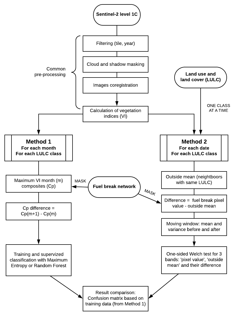
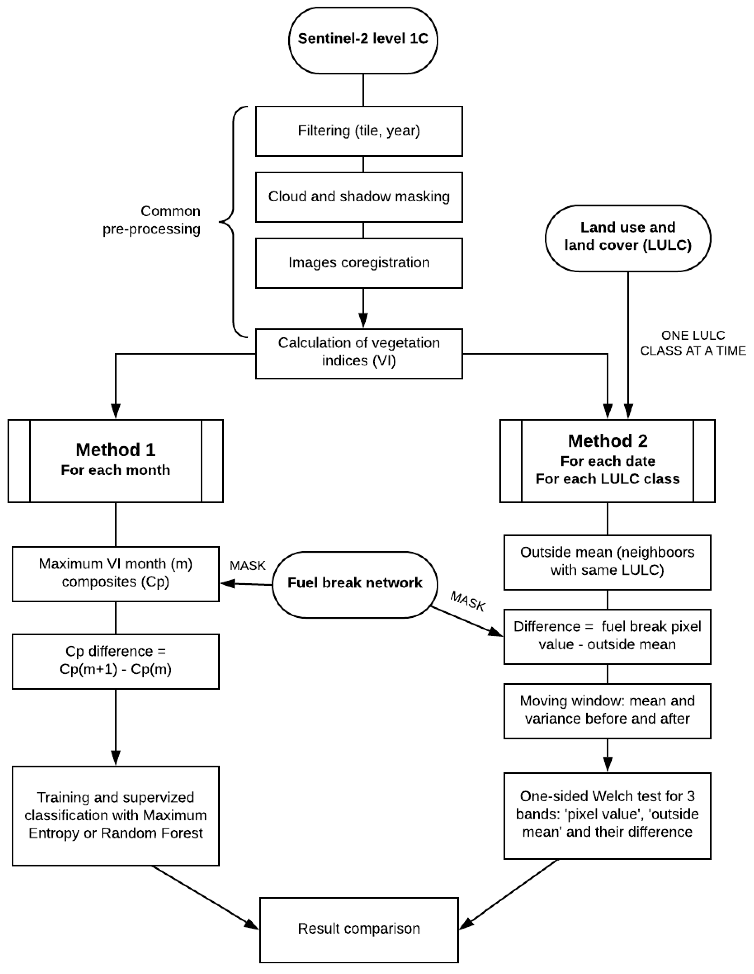
2.2. Two Methodologies for Fuel Break Monitoring

Two complementary methodologies were developed to deal with the phenology of vegetation, the unavailability of reliable training data and the scarcity of clear images (cloud-free and cloud shadow-free). The first method (M1) is based on a pixel-based supervised classification, using monthly composite images differences. The monthly step can be adapted in case of severe unavailability of clear imagery. The second method (M2), computationally more demanding, is based on the detection of statistically significant differences across the time series of satellite data, using a moving window on each pixel. It does not need training data since it uses as a reference the outside neighborhood area of the FB. By these means, it is supposed to avoid false positives due to phenological variations. Imperfect cloud or shadow masking and/or the lack of data are limitations for this technique, since it relies on a statistical test performed on dense time series.
Preprocessing, common to both methods, and processing, specific to each one, were performed in the JavaScript application programming interface (API) of GEE, taking advantage of its powerful cloud interface and computational speed. The workflow (Figure 3) summarizes the main steps described in the following sections.

2.2.1. Common Preprocessing

To mask S2 TOA clouds, cloud shadows and snow, the thresholds and vegetation indices used in the Sen2Cor algorithm [27] were implemented in GEE. S2 TOA images are already georeferenced and their bands aligned [20]. However, some small shifts up to 15 m exist, especially between images from different satellites, which means that images need to be coregistered. If this error is not corrected, pixels in the borders or in the middle road of the FB may shift multiple times from vegetation to no vegetation, increasing the risk of false positives. An image coregistration process was performed for each Sentinel tile and year. A reference image is automatically selected for being free-of-clouds, covering the whole tile, from satellite A (generally better registered according to FB limits) and with the closer date to 1 May. Then, the function displacement of GEE API, which explores pixel correlations [28] between the Red bands of each image and of the reference, was used to estimate the optimal displacement (final parameters used after some tests: maxOffset: 25; patchWidth: 50; stiffness: 5; bicubic resampling). Each band and vegetation index was finally realigned with the function displace (see an example in Figure 4).

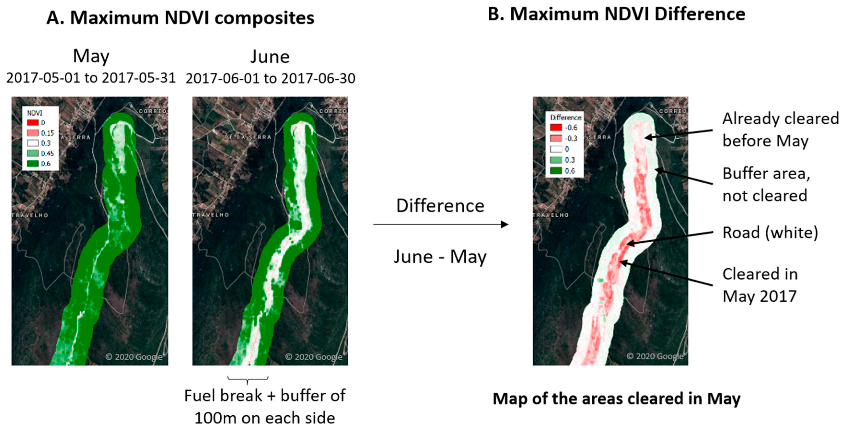
2.2.2. Method 1: Supervised Classification

We first created monthly maximum composites [29]. In GEE, it is possible to create a composite “pixel by pixel” by transforming the image collection into an “Array Image”, where each pixel becomes an Array (or table) with two dimensions: the images and the bands [30]. For each pixel, the images can then be sorted according to the value of one of the bands. We sorted each month collection according to the NDVI band and extracted (for each pixel) the image bands’ values (R, G, B, NDVI and MExG), for which NDVI was the highest. To reduce noise in the data, only images with a “CLOUDY_PIXEL_PERCENTAGE” lower than 30% were used for compositing. The monthly maximum NDVI composites, unlike MExG maximum composites, proved to be an efficient way of enhancing fuel treatment signals and reducing clouds and shadows in the composites. We used the MExG band generated from the same maximum NDVI composite for the next steps of this method. Then, the difference of monthly composites was computed, allowing the detection of fuel treatments on FB (Figure 5).
Two classifiers were used separately: Random Forest and Maximum Entropy (MaxEnt). Both classifiers predict the occurrence of fuel removal interventions given the vegetation indices values. Random Forest [31] generates a large number of decision trees by sampling the training dataset with replacement. To classify a new instance, it collects the classifications and chooses the most voted prediction as the result. MaxEnt estimates probability distributions over an extended feature space for positive events and for all events (background) and minimizes the relative entropy between those two distributions [32]. The ratio of the probability densities is then converted into a likelihood of occurrence for each instance.
Two images were used for training and classification: a vegetation index composite (postdisturbance value) and its difference to the previous monthly composite (disturbance absolute value). The result was a monthly binary intervention/no intervention (INI) classification.

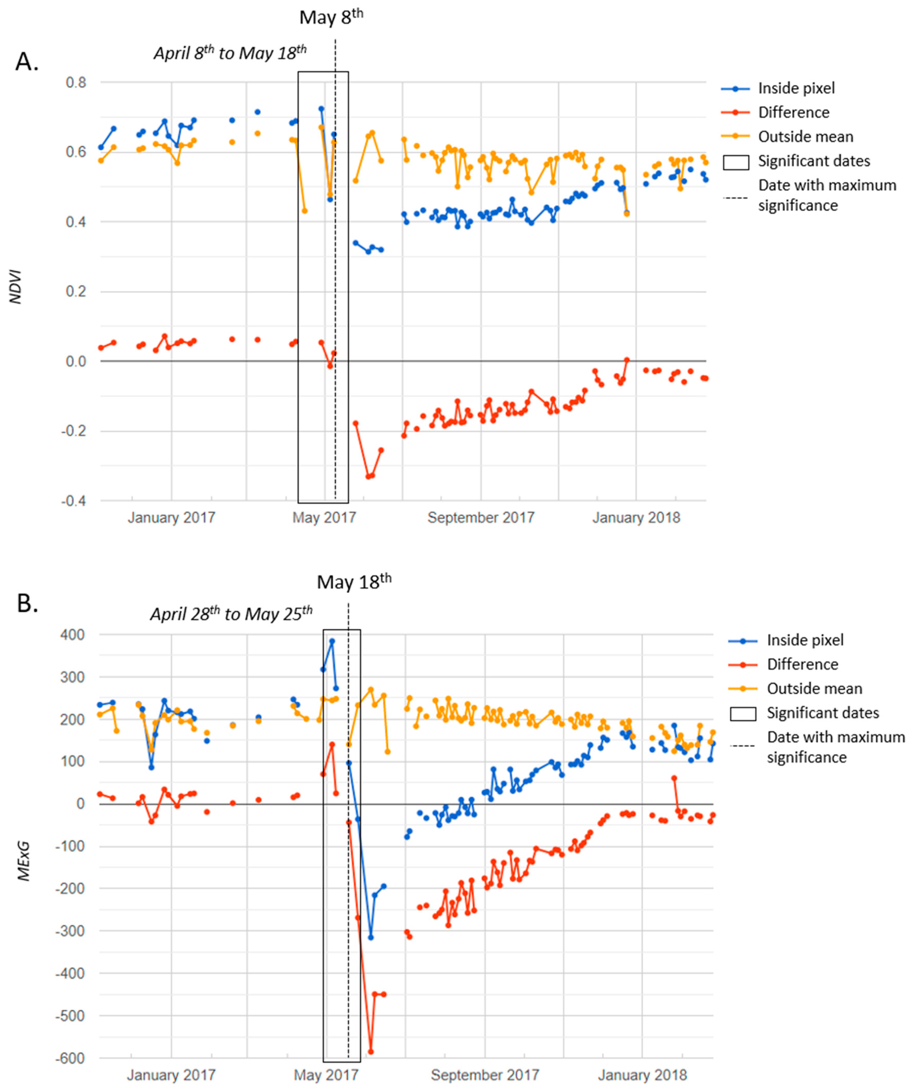
2.2.3. Method 2: Time Series and Welch’s t-Test

Three time series were used: (a) for each vegetation index, the time series of each pixel located inside the FB, “inside pixel”, was computed for one calendar year and elongated by two months, before and after, to encompass the two-month wide moving window that is necessary for the statistical test; (b) the neighboring pixels within 500 m, located outside the FB and of the same land cover class according to 2015 LULC map were used to calculate an “outside mean” time series; (c) the “difference” between those two times series was also computed. When images were from the same date, the maximum value of was kept. The outside mean series interquartile range detected and masked the remaining extreme values in the three series (unmasked clouds or shadows).
A one-sided Welch’s t-test was then applied to each date for the three time series [33]. This test is an adaptation of the Student’s t-test, allowing the identification of significant differences (only significant drops due to the one-sided imposition) between the means of two groups with different sizes and variances. Here, our groups were defined by two temporal moving windows—before and after each date. The minimum number of dates for the test was 2 on each side. We also defined a maximum of 8 dates, to limit the windows’ sample size difference, and a maximum window length of 60 days, to avoid comparing values too far apart but keep enough available dates (some months have only cloudy images). We tried levels of significance α equal to 0.05, 0.005 and 0.0005 to minimize the number of false positives. The result was an INI map for each available date of the year. To discard phenology variations, we considered that an “inside pixel” intervention signal was significant only if, on the same date, it was also significant for “difference” and not for “outside mean” (Figure 6). The first significant date was retained to synthesize results into an annual detection (calendar year). The consistency of observed and detected months of intervention was checked using this first significant date criterion.

2.3. Validation and Results’ Comparison

Validation polygons were delimited for every month, using ground truth and visual image interpretation. Results fell into one of two categories: interventions in the FB were considered positive events (“Yes”) the first month they were observed as such; already treated and never treated areas were considered negative events (“No” intervention).
Monthly INI 2x2 error matrices, which entries are TP the number of true positive events, TN standing for true negative, FP for false positive and FN for false negative events, were obtained from both methods. To compare the methods’ results, suitable accuracy metrics were chosen: overall accuracy, precision, recall and F1-score [30,31]. The overall accuracy expresses the proportion of referenced sites (validation pixels) that were mapped correctly in the dataset:
Overall accuracy = (TP + TN)/(TP + TN + FP + FN).
Precision and recall metrics were computed for each category reflecting the occurrence of false positives and negatives. For one category (a fuel treatment detected, “Yes”, or no fuel treatment, “No”), the precision gave the fraction of correctly classified events among retrieved events, here for the category “Yes”:
Precision = TP/(TP + FP) = 1 − commission error.
A higher precision meant that the classifier had a good behavior avoiding false positives events. Among one category, the recall measured the fraction of relevant events that was classified as such, for category “Yes”:
Recall = TP/(TP + FN) = 1 − omission error.
The recall showed the ability of the classifier to not detect false negatives. The F1-score, that ranged between 0 (when either Precision or Recall is zero) and 1 (when both are 1), was a balance between precision and recall that measured the accuracy of the classification of each category:
F1-score = 2 × (Precision × Recall)/(Precision + Recall)
The accuracy of the methods was compared at two time steps. At the monthly step, the accuracy metrics were calculated from the sum of the twelve monthly INI error matrices from one year. For annual comparisons, monthly maps were aggregated: a pixel observed or detected positive one or more times during the year was considered a positive event; if it was never detected positive, it stayed negative. Those annual binary maps of results and validations were used to compute annual INI error matrices and the corresponding accuracy metrics.

3. Results

Four classifier–vegetation index pairs were tested in M1. Table 3 compares the accuracy metrics for each pair, at annual and monthly steps. Recall, Precision and F1-score metrics are given separately for the two categories: positive events (fuel treatment detected: “Yes”) and negative events (“No”). Metrics revealed that MaxEnt performed better than RF, and NDVI better than MExG. The best couple, MaxEnt-NDVI, could detect fuel treatment with a 54% precision and 69% recall on a yearly basis. For positive events, the monthly F1-score was lower than the annual score (45% against 61%). A deeper analysis of results revealed that this was mainly due to a difference of one or two months earlier or later with regard to the validation date.
Two vegetation indices and three levels of significance were tested with M2 (Table 4). NDVI and MExG gave close results. For both, the precision tended to increase inversely to α, at the expense of the recall. The metrics showed an improved precision in comparison to the best pair of M1 (MaxEnt-NDVI), but a lower recall.
The detection of positive FB treatments was less accurate in the forest areas than in shrublands, for both methods (Table 5). On the contrary, negative events lost accuracy in shrublands, potentially because of higher phenological variations.
Figure 7 shows an example of map results for both methods in Serra de Aires, a shrubland. We can see the improvement of M2 monthly detection results when α decreased (NDVI from α = 0.05 to α = 0.0005). The visual comparison of the M2 best results (NDVI and MExG for α = 0.0005) with M1 best results (MaxEnt NDVI and RF NDVI) indicate that M2 was able to distinguish the pixel of the central road from the rest of the FB (middle white lines).
In dense forest areas, such as the maritime pine forest of Amarante (Figure 8), the two methodologies were able to detect maintenance operations alongside roads, where the canopy cover was the thinnest.
In Proença-a-Nova study area (Figure 9), there was a 3 month gap between cuttings and the removal of vegetation debris. This situation was frequent and was harder to identify by image interpretation or using M1, while fuel treatments months were correctly identified with M2.
MExG index seemed to be more sensitive than NDVI to understory clearing under dense canopy cover (Figure 8, rectangle of understory cut on October–November near some houses; Figure 9, fuel treatments marked in June–July in the W–E oriented FB).
In cork oaks open woodlands (Figure 10), planted in drier areas and poorer soils, M1 (MaxEnt NDVI) detected interventions in March (around the wind turbines) and in April 2017. Fuel treatments actually happened the previous year, but the new herbaceous vegetation rapidly dried when the temperature became high and precipitations became scarce: M1 is sensitive to phenology variations. On the contrary, M2, by comparing pixel values with their neighborhood of same land cover, avoided these kinds of false positives.
This characteristics of M2 can be a disadvantage when dealing with agricultural landscapes (Figure 11, land cover in yellow). The comparisons of values of the same agricultural field inside and outside the FB prevents M2 from detecting the fuel reduction insured by harvests in May–June.

4. Discussion

The methodologies implemented permitted a highly automated detection of fuel treatments on FB. The resulting accuracies can be considered representative for the whole of Portugal, since five areas with various conditions and land cover were used, even northern areas (Amarante and Manteigas) that have frequent cloud cover that makes fuel treatment detection difficult with either method.
M1 needs reliable training data and efficiently deals with phenology by comparing composites at a short time step of one month. M2 deals with phenology by a spatial comparison using neighborhood pixels of the same land cover outside the FB. This last method does not need training data, nor a specific threshold or a good knowledge of the species and of their spectral characteristics. On the other hand, it requires the specification of a significance level and more computational resources. Its accuracy also depends on the length of the window chosen. M2 relies on spectral data before and after potential fuel treatments, which makes it less reactive than M1. In GEE, the processing of M2 takes between 3 and 4 h per area, compared to 30 min with M1.
M2 produced good results for smaller levels of significance than the commonly used 0.05 (Table 4 and Figure 7). For this level of significance, it was too sensitive to short-term greenness variations due to vegetation response to rainfall and drought episodes. Multiple false positives or early detections were avoided by lowering the level significance to 0.005 or even 0.0005. A good balance between the number of clear available images and the capability of mitigating the effects of phenological variations was found for a window length of 60 days.
A comparison of the detection in forests and shrublands, the two main land covers of FBs (see Table 1), showed that fuel treatments were detected less efficiently in forest areas (Table 5). This was expected, since in this last case, only a few pixels alongside the road, with a limited tree cover, can inform on the state of the understory. This difference could also suggest that M1 (supervised classification) could be improved by training and classifying shrublands and forest areas separately, which was not performed in this study.
The delineation of the validation dataset was mainly performed with visual image interpretation, which originated a lack of spatial precision, as it can been seen in the validation shapes of Figure 8. On the contrary, S2 10 m resolution and the re-alignment preprocessing step allowed the detection of treatments in dense forest areas (Figure 8 and Figure 9) and the distinction of roads from shrubland pixels with M2 (Figure 7 and Figure 10). This difference in spatial precision between data and validation could have led to an underestimation of the detection power of both methods, especially in forest areas. High resolution ground truth data would be necessary to take full advantage of the satellite image spatial resolution, which could be used both in classification training and validation.
The objective of this study was an operational fuel monitoring in FB. Fuel treatment maps will be used for prevention planning and firefighting, which require high precision (few false positives). On this point, the second methodology gave more satisfying results. M2 resulted in higher precision for positive events (M1: 54%; M2: 74%, at yearly level) and lower recall (M1: 69%; M2: 40%) (more false negatives). However, M2 also resulted in a lower F1-score (M1: 61%; M2: 52%).
In a recent study, an object-based approach for FB fuel treatment detection suggested that most discriminant vegetation indices for classification were based on visible bands, using B05, the excess of green and excess of red indices [19]. Our comparison between NDVI and MExG results did not confirm this hypothesis. NDVI gave better results with M1, while the accuracies were similar to M2′s. This difference could be due to different test areas and the inclusion in the present work of more varied ecosystems, from North to South of Portugal; more years; and more extensively forested areas.

5. Conclusions

The two pixel-based methods allow good detection of fuel break maintenance operations. Both methods have advantages and disadvantages in their applicability and result accuracy. M1, a supervised classification, needs reliable training data, while M2, based on exhaustive time series datasets of two months, is almost fully automatic but requires more processing resources. This latter limitation can be overcome by using a powerful cloud-based platform such as GEE, as was performed in the present study. Compared to M1, M2 gave a better precision for a lower recall, which could be considered more relevant for the operational goal of this study: mapping fuel treatments to insure efficient prevention and safe firefighting.
Overall, NDVI gave better results than the visible based index MExG for MaxEnt and RF supervised classifiers (M1). For a level of significance of 0.0005, NDVI and MExG displayed similar results for M2.
Compared to the object-based approach, the pixel-based approach does not require the delineation of polygons before detection and is thus more adapted to automated large scale monitoring of maintenance operations for the full ICNF FB network.
Future steps will consist of efficiently aggregating the positive event pixels into objects to monitor the recovery dynamics of the treated vegetation. Ultimately, an automated system will be developed to alert for fuel reduction intervention necessity.

Author Contributions

Conceptualization, V.A., J.M.N.S., J.E.P.-P., A.M., J.M.C.P. and M.L.C.; methodology, V.A. and J.M.N.S.; software, V.A.; validation, V.A., J.M.N.S., J.E.P.-P. and A.M.; formal analysis, V.A., J.M.N.S., J.E.P.-P., A.M., J.M.C.P. and M.L.C.; investigation, V.A., J.M.N.S., J.E.P.-P., A.M., J.M.C.P. and M.L.C.; writing—original draft preparation, V.A. and J.M.N.S.; writing—review and editing, V.A., J.M.N.S., J.E.P.-P., A.M., J.M.C.P. and M.L.C; supervision, A.M. and J.M.N.S.; project administration, A.M., J.M.N.S.; funding acquisition, A.M., J.M.N.S. All authors have read and agreed to the published version of the manuscript.

Funding

This research was funded by Fundação de Ciências e Tecnologia (FCT) under the framework of projects FUELMON (PTDC/CCI-COM/30344/2017) and foRESTER (PCIF/SSI/0102/2017). The Forest Research Centre and the Centre of Technology and Systems/UNINOVA are research units funded by FCT (UIDB/00239/2020; UIDB/00066/2020).

Acknowledgments

The authors would like to acknowledge the Portuguese Institute for Nature and Forests Conservation (Instituto de Conservação da Natureza e das Florestas, ICNF) for introducing our team to this research topic and supplying data regarding the maintenance operations.

Conflicts of Interest

The authors declare no conflict of interest.

References

  1. Shukla, P.R.; Skea, J.; Calvo Buendia, E.; Masson-Delmotte, V.; Pörtner, H.-O.; Roberts, D.C.; Zhai, P.; Slade, R.; Connors, S.; van Diemen, R.; et al. Climate Change and Land: An IPCC Special Report on Climate Change, Desertification, Land Degradation, Sustainable Land Management, Food Security, and Greenhouse Gas Fluxes in Terrestrial Ecosystems; IPCC: Geneva, Switzerland, 2019. [Google Scholar]
  2. Camia, A.; Liberta, G.; San-Miguel-Ayanz, J. Modeling the Impacts of Climate Change on Forest Fire Danger in Europe; Joint Research Centre (European Commission): Brussels, Belgium, 2017. [Google Scholar] [CrossRef]
  3. San-Miguel-Ayanz, J.; Durrant, T.; Boca, R.; Libertà, G.; Branco, A.; De Rigo, D.; Ferrari, D.; Maianti, P.; Vivancos, T.A.; Oom, D.; et al. Forest Fires in Europe, Middle East and North Africa 2018; EUR 29856 EN; Publications Office of the European Union: Luxembourg, 2019; ISBN 978-92-76-11234-1. [Google Scholar] [CrossRef]
  4. Silva, J.M.N.; Moreno, M.V.; Le Page, Y.; Oom, D.; Bistinas, I.; Pereira, J.M.C. Spatiotemporal trends of area burnt in the Iberian Peninsula, 1975–2013. Reg. Environ. Chang. 2019, 19, 515–527. [Google Scholar] [CrossRef]
  5. Beighley, M.; Hyde, A.C. Portugal Wildfire Management in a New Era. Assessing Fire Risks, Resources and Reforms. 2018. Available online: https://www.isa.ulisboa.pt/files/cef/pub/articles/2018-04/2018_Portugal_Wildfire_Management_in_a_New_Era_Engish.pdf (accessed on 4 September 2020).
  6. Viedma, O.; Moity, N.; Moreno, J.M. Changes in landscape fire-hazard during the second half of the 20th century: Agriculture abandonment and the changing role of driving factors. Agric. Ecosyst. Environ. 2015, 207, 126–140. [Google Scholar] [CrossRef]
  7. Plano Nacional de Defesa da Floresta Contra Incêndios–ICNF. Available online: http://www2.icnf.pt/portal/florestas/dfci/planos/PNDFCI (accessed on 13 April 2020).
  8. Syphard, A.D.; Keeley, J.E.; Brennan, T.J. Factors affecting fuel break effectiveness in the control of large fires on the Los Padres National Forest, California. Int. J. Wildland Fire 2011, 20, 764–775. [Google Scholar] [CrossRef]
  9. Oliveira, T.M.; Barros, A.M.G.; Ager, A.A.; Fernandes, P.M. Assessing the effect of a fuel break network to reduce burnt area and wildfire risk transmission. Int. J. Wildland Fire 2016, 25, 619–632. [Google Scholar] [CrossRef]
  10. Ministério da Agricultura do Mar do Ambiente e do Ordenamento do Território. Divisão de Proteção Florestal e Valorização de Áreas Públicas (DPFVAP). Manual de Rede Primária; ICNF: Lisbon, Portugal, 2014. [Google Scholar]
  11. Ministério da Agricultura do Desenvolvimento Rural e das Pescas Decreto-Lei 124/2006, 2006-06-28. Available online: https://data.dre.pt/eli/dec-lei/124/2006/06/28/p/dre/pt/html (accessed on 1 May 2020).
  12. Tewkesbury, A.P.; Comber, A.J.; Tate, N.J.; Lamb, A.; Fisher, P.F. A critical synthesis of remotely sensed optical image change detection techniques. Remote Sens. Environ. 2015, 160, 1–14. [Google Scholar] [CrossRef] [Green Version]
  13. Lu, D.; Li, G.; Moran, E. Current situation and needs of change detection techniques. Int. J. Image Data Fusion 2014, 5, 13–38. [Google Scholar] [CrossRef]
  14. Tarantino, C.; Adamo, M.; Lucas, R.; Blonda, P. Change detection in (semi-) natural grassland ecosystems for biodiversity monitoring using open data. In Proceedings of the IEEE International Geoscience and Remote Sensing Symposium (IGARSS 2018), Valencia, Spain, 30 June 2018; pp. 8981–8984. [Google Scholar]
  15. Wang, Z.; Yao, W.; Tang, Q.; Liu, L.; Xiao, P.; Kong, X.; Zhang, P.; Shi, F.; Wang, Y. Continuous change detection of forest/grassland and cropland in the loess plateau of China using all available landsat data. Remote Sens. 2018, 10, 1775. [Google Scholar] [CrossRef] [Green Version]
  16. Kolecka, N.; Ginzler, C.; Pazur, R.; Price, B.; Verburg, P.H. Regional scale mapping of grassland mowing frequency with sentinel-2 time series. Remote Sens. 2018, 10, 1221. [Google Scholar] [CrossRef] [Green Version]
  17. Johansen, K.; Phinn, S.; Taylor, M. Mapping woody vegetation clearing in Queensland, Australia from Landsat imagery using the Google Earth Engine. Remote Sens. Appl. Soc. Environ. 2015, 1, 36–49. [Google Scholar] [CrossRef]
  18. Bekkema, M.E.; Eleveld, M. Mapping grassland management intensity using sentinel-2 satellite data. J. Geogr. Inf. Sci. 2018, 6, 194–213. [Google Scholar] [CrossRef]
  19. Pereira-Pires, J.E.; Aubard, V.; Ribeiro, R.A.; Fonseca, J.M.; Silva, J.M.N.; Mora, A. Semi-automatic methodology for fire break maintenance operations detection with sentinel-2 imagery and artificial neural network. Remote Sens. 2020, 12, 909. [Google Scholar] [CrossRef] [Green Version]
  20. European Space Agency (ESA). Sentinel-2 User Handbook; European Space Agency: Brussels, Belgium, 2015. [Google Scholar]
  21. Gorelick, N.; Hancher, M.; Dixon, M.; Ilyushchenko, S.; Thau, D.; Moore, R. Google Earth Engine: Planetary-scale geospatial analysis for everyone. Remote Sens. Environ. 2017, 202, 18–27. [Google Scholar] [CrossRef]
  22. Direção-Geral do Território. Especificações técnicas da Carta de uso e Ocupação do Solo de Portugal Continental para 1995, 2007, 2010 e 2015. Relatório Técnico; Direção-Geral do Território: Lisbon, Portugal, 2018. [Google Scholar]
  23. Cerasoli, S.; e Silva, F.C.; Silva, J.M. Temporal dynamics of spectral bioindicators evidence biological and ecological differences among functional types in a cork oak open woodland. Int. J. Biometeorol. 2016, 60, 813–825. [Google Scholar] [CrossRef] [PubMed]
  24. Tucker, C.J. Red and photographic infrared linear combinations for monitoring vegetation. Remote Sens. Environ. 1979, 8, 127–150. [Google Scholar] [CrossRef] [Green Version]
  25. Hamuda, E.; Glavin, M.; Jones, E. A survey of image processing techniques for plant extraction and segmentation in the field. Comput. Electron. Agric. 2016, 125, 184–199. [Google Scholar] [CrossRef]
  26. Burgos-Artizzu, X.P.; Ribeiro, A.; Guijarro, M.; Pajares, G. Real-time image processing for crop/weed discrimination in maize fields. Comput. Electron. Agric. 2011, 75, 337–346. [Google Scholar] [CrossRef] [Green Version]
  27. Sentinel Online. Level-2A Processing Overview–Sentinel-2 MSI–Technical Guide–Sentinel Online. Available online: https://earth.esa.int/web/sentinel/technical-guides/sentinel-2-msi/level-2a/algorithm (accessed on 13 April 2020).
  28. Google Earth Engine. Registering Images. Available online: https://developers.google.com/earth-engine/register?hl=fr (accessed on 13 April 2020).
  29. Holben, B.N. Characteristics of maximum-value composite images from temporal AVHRR data. Int. J. Remote Sens. 1986, 7, 1417–1434. [Google Scholar] [CrossRef]
  30. Google Earth Engine. Arrays and Array Images. Available online: https://developers.google.com/earth-engine/arrays_array_images?hl=fr (accessed on 13 April 2020).
  31. Breiman, L. Random Forests. Mach. Learn. 2001, 45, 5–32. [Google Scholar] [CrossRef] [Green Version]
  32. Elith, J.; Phillips, S.J.; Hastie, T.; Dudík, M.; Chee, Y.E.; Yates, C.J. A statistical explanation of MaxEnt for ecologists. Divers. Distrib. 2011, 17, 43–57. [Google Scholar] [CrossRef]
  33. Campagnolo, M.L.; Oom, D.; Padilla, M.; Pereira, J.M.C. A patch-based algorithm for global and daily burned area mapping. Remote Sens. Environ. 2019, 232. [Google Scholar] [CrossRef]
Figure 1. Transversal view of a model fuel break. The total width is 125 m. The distance between tree crowns decreases with the distance to the road. The first 10 m on the sides of the road have no vegetation. Adapted from [10].
Remotesensing 12 02879 g001
Figure 2. Locations of the five study areas in Portugal.
Remotesensing 12 02879 g002
Figure 3. Flowchart including the common preprocessing and the two methodologies.
Remotesensing 12 02879 g003
Figure 4. Time series (A). before and (B). after coregistration of three points located on an unpaved road of the fuel break (center, in blue), 20 m on its left (red) and 20 m on its right (orange), with (C). the location of the three points on an aerial view of the fuel break. The images of the tile are all coregistered using a reference image (vertical dash line).
Remotesensing 12 02879 g004
Figure 5. Example in Serra de Candeeiros (shrubs) of: (A) two monthly maximum NDVI composites; (B) their difference (June composite–May composite).Training datasets were established using the information provided by ICNF on the location of fuel treatments, and also through visual image interpretation. The training dataset contains the values of 20,000 points inside and outside the FB, from all months of the year, one-third of which correspond to locations where fuel removal interventions occurred.
Remotesensing 12 02879 g005
Figure 6. Example of the three time series (“inside pixel” in blue, “outside mean” in yellow, “difference” in red) in Serra de Candeeiros (shrubs) for (A). NDVI and (B). MExG, with all significant dates (black rectangle) and the maximum significant date (vertical dash line), for a one-sided Welch’s test with α = 0.05.
Remotesensing 12 02879 g006
Figure 7. Results in Serra de Candeeiros in 2017: A. land cover; B. results from Method 1 and Method 2. The validation figure indicates the monthly fuel treatments assessed by image interpretation.
Remotesensing 12 02879 g007
Figure 8. Results in a pine forest area in Amarante municipality in 2018: A. land cover; B. results of Method 1, MaxEnt NDVI classification, and Method 2, NDVI and MExG statistical detection with α = 0.0005.
Remotesensing 12 02879 g008
Figure 9. Results in a pine forest area of Proença-a-Nova for the year 2019: A. land cover; B. results of Method 1, MaxEnt NDVI classification, and Method 2, NDVI and MExG statistical detection with α = 0.0005. In the part of the fuel break oriented N-S, the vegetation was first slashed and removed three months later; validation gives the month of the cut.
Remotesensing 12 02879 g009
Figure 10. Results in a cork oak woodland area of Serra de Caldeirão in 2017: A. land cover; B. results of Method 1, MaxEnt NDVI classification, and Method 2, NDVI and MExG statistical detection with α = 0.0005.
Remotesensing 12 02879 g010
Figure 11. Results in Manteigas for the year 2016: A. Land cover; B. results of Method 1, MaxEnt NDVI classification, and Method 2, NDVI and MExG statistical detection with α = 0.0005.
Remotesensing 12 02879 g011
Table 1. Simplified land cover classification, adapted from [22], with area and relative area in the Portuguese fuel break network.
NameOriginal Class NumberDetailsArea (ha)Relative Area (%)
Artificialized lands1.Continuous and discontinuous urban fabric, industries, parks, airports, historical areas, leisure infrastructures and golf fields.17473.6
Agriculture2.Permanent and temporary agriculture fields, some with natural areas, including orchards, olive groves and vineyards.549711.4
Forest3.1.Mainly cork oaks, holm oaks, eucalyptus, stone pine and maritime pine. 24,01749.7
Agroforestry2.4.4.Oaks or pines agroforestry systems.6631.4
Shrublands3.2.2. 13,62128.2
Herbaceous vegetation2.3. and 3.2.1.Permanent pasture and natural herbaceous18693.9
Sparse vegetation3.3. 7871.6
Water4. and 5.Inland water and wetlands1450.3
Total 48,346100
Table 2. Study sites studied years, fuel break area, land cover composition and climate conditions.
Study AreaYears Area (ha)Forest (%)Shrubs (%)P (mm) *maxT (°C) *
Serra de Caldeirão2016–2017205.258.74080019
Manteigas2016–2017204.63142.2140014
Serra de Candeeiros2017–2018398.620.961.9120018
Amarante2018–201997.690.38.3160016
Proença-a-Nova2018–201920279.219.2110020
Total2016–2019110846.541.7
* Mean annual precipitation (P) and maximum temperature (maxT) based on the 1971–2000 climate normals (source: IPMA).
Table 3. Global accuracy results for Method 1, at annual and monthly steps.
Classifier and IndexMaxEnt NDVIMaxEnt MExGRF NDVIRF MExG
Fuel treatment detectedYesNoYesNoYesNoYesNo
AnnualPrecision (%)5487359543873392
Recall (%)6978963273649429
F1-Score (%)6182514854744944
Overall accuracy (%)75506646
MonthlyPrecision (%)389989925991199
Recall (%)5698837855966387
F1-Score (%)4598158835981893
Overall accuracy (%)97799587
Table 4. Global accuracy results for Method 2, at annual and monthly steps.
Vegetation index and Level of significanceNDVI
0.05
NDVI
0.005
NDVI
0.0005
MExG
0.05
MExG
0.005
MExG
0.0005
Fuel treatment detectedYesNoYesNoYesNoYesNoYesNoYesNo
AnnualPrecision (%)378756837480358350836682
Recall (%)805057834095774560764791
F1-Score (%)516357835287485954795586
Overall accuracy (%)587679547279
MonthlyPrecision (%)109826985298109827984598
Recall (%)219627982899239533983299
F1-Score (%)139727983799149730983799
Overall accuracy (%)949798949698
Table 5. Comparison of the accuracies obtained for two land cover types: Forest and Shrubs; for the pair MaxEnt-NDVI from Method 1 (M1) and the indices NDVI and MExG from Method 2 with α = 0.0005, at annual and monthly steps.
Land cover and MethodForest M1Forest NDVIForest MExGShrubs M1Shrubs NDVIShrubs MExG
Fuel treatment detectedYesNoYesNoYesNoYesNoYesNoYesNo
AnnualPrecision (%)459069885789608483787880
Recall (%)628243955191717647955592
F1-Score (%)528653915490658060866f486
Overall accuracy (%)788583757980
MonthlyPrecision (%)349954994199479958985398
Recall (%)5298331003799629833993799
F1-Score (%)419941993899539842994499
Overall accuracy (%)989898979797

