Examining the Roles of Spectral, Spatial, and Topographic Features in Improving Land-Cover and Forest Classifications in a Subtropical Region

Abstract

Many studies have investigated the effects of spectral and spatial features of remotely sensed data and topographic characteristics on land-cover and forest classification results, but they are mainly based on individual sensor data. How these features from different kinds of remotely sensed data with various spatial resolutions influence classification results is unclear. We conducted a comprehensively comparative analysis of spectral and spatial features from ZiYuan-3 (ZY-3), Sentinel-2, and Landsat and their fused datasets with spatial resolution ranges from 2 m, 6 m, 10 m, 15 m, and to 30 m, and topographic factors in influencing land-cover classification results in a subtropical forest ecosystem using random forest approach. The results indicated that the combined spectral (fused data based on ZY-3 and Sentinel-2), spatial, and topographical data with 2-m spatial resolution provided the highest overall classification accuracy of 83.5% for 11 land-cover classes, as well as the highest accuracies for almost all individual classes. The improvement of spectral bands from 4 to 10 through fusion of ZY-3 and Sentinel-2 data increased overall accuracy by 14.2% at 2-m spatial resolution, and by 11.1% at 6-m spatial resolution. Textures from high spatial resolution imagery play more important roles than textures from medium spatial resolution images. The incorporation of textural images into spectral data in the 2-m spatial resolution imagery improved overall accuracy by 6.0–7.7% compared to 1.1–1.7% in the 10-m to 30-m spatial resolution images. Incorporation of topographic factors into spectral and textural imagery further improved overall accuracy by 1.2–5.5%. The classification accuracies for coniferous forest, eucalyptus, other broadleaf forests, and bamboo forest can be 85.3–91.1%. This research provides new insights for using proper combinations of spectral bands and textures corresponding to specifically spatial resolution images in improving land-cover and forest classifications in subtropical regions.

1. Introduction

The subtropical ecosystem in China plays an important role in the global carbon cycle because of its abundant forest cover and high carbon sequestration [1]. This region is characterized by high heterogeneity of land-cover types from frequent disturbances due to high population density and natural disasters (e.g., typhoon, drought). High precipitation and temperatures along with complex topographic conditions favor the growth of various tree species, resulting in rich tree diversity and complex terrestrial ecosystems. A prominent characteristic of this region is the large areas of plantations, including Chinese fir, eucalyptus, pines, and many precious timber types, which have high carbon sequestration rates [2,3,4]. Therefore, accurate mapping of the spatial distribution of different forest types is needed for better decisions to improve forest management and estimate forest carbon stocks [5].

Mapping forest distribution with remote-sensing technologies has long been an important research topic since satellite data became available in the early 1970s [6,7]. In the 1980s and 1990s, forest mapping was produced using visual interpretation of aerial photographs or topographic maps supported by field surveys and using automatic classification with statistic-based parametric classifiers based on medium spatial resolution images (mainly Landsat MSS (Multispectral Scanner) and TM (Thematic Mapper)) [8,9,10,11]. More recently, machine learning algorithms and even deep learning based on multisource data have been used [12,13,14,15]. Since entering the 21st century, as high spatial resolution images such as IKONOS, Quickbird, and WorldView have become easily accessible, many studies have explored the use of those images for mapping detailed forest classes, even at tree species levels [16,17,18,19,20], although medium spatial resolution is still the dominant form of remotely sensed data [21,22]. With the availability of Google Earth Engine and cloud computing platforms, medium spatial resolution images, such as Sentinel-2 and Landsat, are used for mapping land-cover distribution at national and global scales [23,24,25,26]. As different sensor and ancillary data became available, many technologies such as integration of spectral, spatial, and temporal features of remotely sensed data, integration of different sensor data (e.g., multispectral and panchromatic data, optical sensor, and radar) [27,28,29,30], and combinations of remotely sensed and ancillary data (e.g., digital elevation model, population density) were explored [11,19,31,32].

The medium spatial resolution images such as Landsat, Sentinel-2, ASTER (Advanced Spaceborne Thermal Emission and Reflection Radiometer), SPOT (Satellite Pour l’Observation de la Terre), and ALOS PALSAR (Advanced Land Observing Satellite/Phased Array type L-band Synthetic Aperture Radar) are dominant sources for land-cover and forest mapping, but the classification results vary, depending on the classification system and classifiers used, as well as the complexity of landscapes under investigation [10,33]. Landsat, with its suitable spectral and spatial resolutions and having the longest continuously available satellite data, provides the most widely used sources for land-cover or forest mapping [7,13,21,34]. Spectral features are the most important variables for forest classification because of the unique spectral responses of different forest types in proportion to the electromagnetic spectrum [5,35,36]. Proper integration of textures into spectral bands is helpful for improving land-cover classification [5,18,37], and the forest stand structure features, which are special characteristics inherent in forest types, are valuable for forest classification [19,38]. However, obtaining such information requires more data from forest inventories, which is often difficult and costly. Because of relatively small patch sizes of plantations in subtropical regions, the mixed pixel problem at 30-m spatial resolution of Landsat imagery can be an important factor resulting in poor classification. A common approach to reduce the mixed pixel problem is to conduct data fusion, which integrates the rich spectral information of medium resolution data and fine spatial information of high spatial resolution data (see review papers in [10,39,40,41]). Previous research indicated that data fusion of Landsat multispectral and panchromatic bands or Landsat and radar can improve land-cover classification performance [10,42]. Currently, easy access to different remotely sensed data with various spectral and spatial resolutions makes such integration of different data sources possible to improve land-cover or forest classification [26,27,33]. Another direct solution to reduce the mixed pixel problem is to use high spatial resolution images from sensor data such as Worldview, Pleiades, Quickbird, and GaoFen–1/2/3, which have been available since 2000 [43,44].

The high spatial resolution images are important data sources for detailed land-cover classification due to their rich spatial information. However, the limited number of spectral bands in most high spatial resolution images—only four bands within the range of visible and near-infrared (NIR) wavelengths without shortwave infrared (SWIR) spectral bands—make differentiating forest or tree species types difficult due to the complex tree species composition and heterogeneity of stand structure [44,45]. The key is to properly employ the spatial features into a forest classification procedure. In general, segmentation and texture are two common approaches to use spatial features from remotely sensed data and have been proven effective in improving land-cover [37,46,47] and forest/species classification, even in small patch sizes [19]. Use of segmentation is often involved in the object-oriented classification approach, for which the development of proper segment images is one of the critical steps, while texture is calculated from a specific image based on a selected window size using certain approaches such as variance and contrast [35,46]. The texture measures based on gray-level co-occurrence matrix (GLCM) are often used to extract textural images because of the easy implementation with the statistically based calculation [37]. The key in using textural images is to identify the proper combination of textural images that can effectively enhance the separation of different forest types under investigation [19,20,37].

Topographic data are also important for improving forest classification in mountainous regions [35,48,49,50]. Topography greatly influences the distribution of vegetation species [51,52]. Different elevations, slopes, and aspects create various environmental conditions such as solar radiation, temperature, moisture, and soil fertility [53,54], all of which contribute to the species’ diversity and distribution. Previous research has indicated that incorporation of topographic factors with spectral data into the classification procedure can improve land-cover classification accuracy [19,49,55,56]. In general, these topographic characteristics are calculated from digital elevation model (DEM) data. Topographic factors are often used in three ways: (1) To reduce the impacts of different terrain conditions on surface reflectance through use of topographic correction approaches such as Minnaert, C-correction, and statistical-empirical models [57,58]; (2) to increase the number of variables as extra bands for use during image classification [19]; and (3) to conduct post-processing of the classified image by using expert rules [35]. One important thing is to obtain suitable spatial resolution of DEM data. At present, the DEM data are often downloaded from SRTM (Shuttle Radar Topography Mission), ASTER, and ALOS at no cost. These DEM data are commonly used with Landsat images because of the similarity of pixel sizes but may not be suitable for high spatial resolution images such as Quickbird. Therefore, in recent years, many high spatial resolution DEM data have been developed from airborne Lidar or stereo images [19].

Optical sensor data have spectral, spatial, and temporal features, but the effectiveness of using these features from different sensor data with various spatial resolutions and their roles in improving land-cover and forest classification have not been fully examined. In mountainous areas, how to effectively use topographic factors to improve individual forest classification remains unanswered. Therefore, the objective of this research was to better understand the roles of spectral, spatial, and topographic features in improving forest classification in a subtropical region. Specifically, the research aimed to explore (1) how different spatial and spectral resolutions influence land-cover and forest classification, (2) how fusion of different spatial resolutions or sensor data improves land-cover and forest classification, and (3) how incorporation of topographic factors into optical sensor data improves land-cover and forest classification. Through a comprehensive analysis of data scenarios covering combinations of spectral, spatial, and topographic features in different ways, we can better understand how to design a suitable classification procedure that corresponds to a specific data source and classification system in a subtropical ecosystem to produce an optimal classification result. The new contribution of this research is to better understand the design of a classification procedure and the selection of spectral, spatial, and topographic features suitable for specific data sets and classification systems under investigation.

2. Materials and Methods

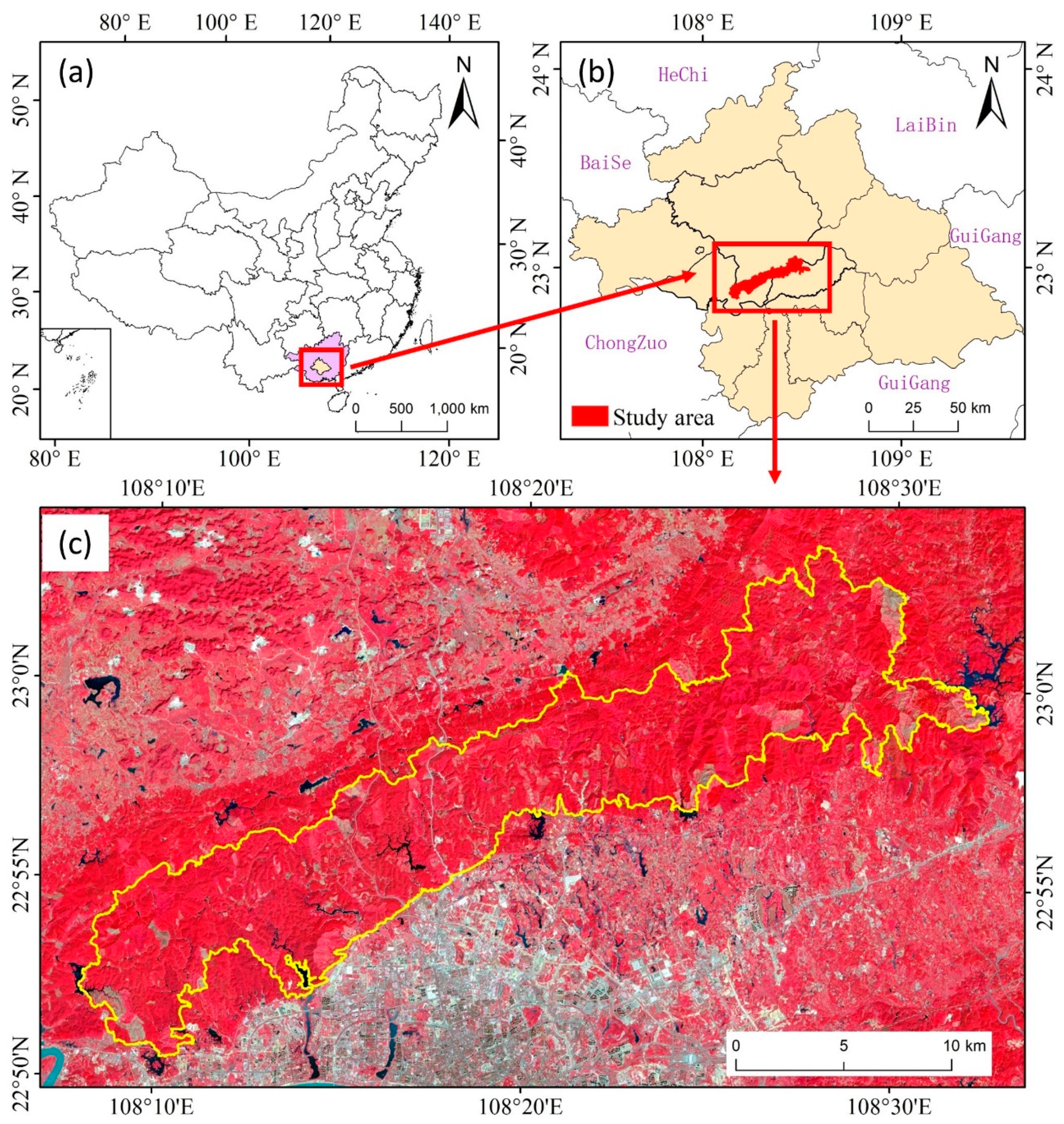
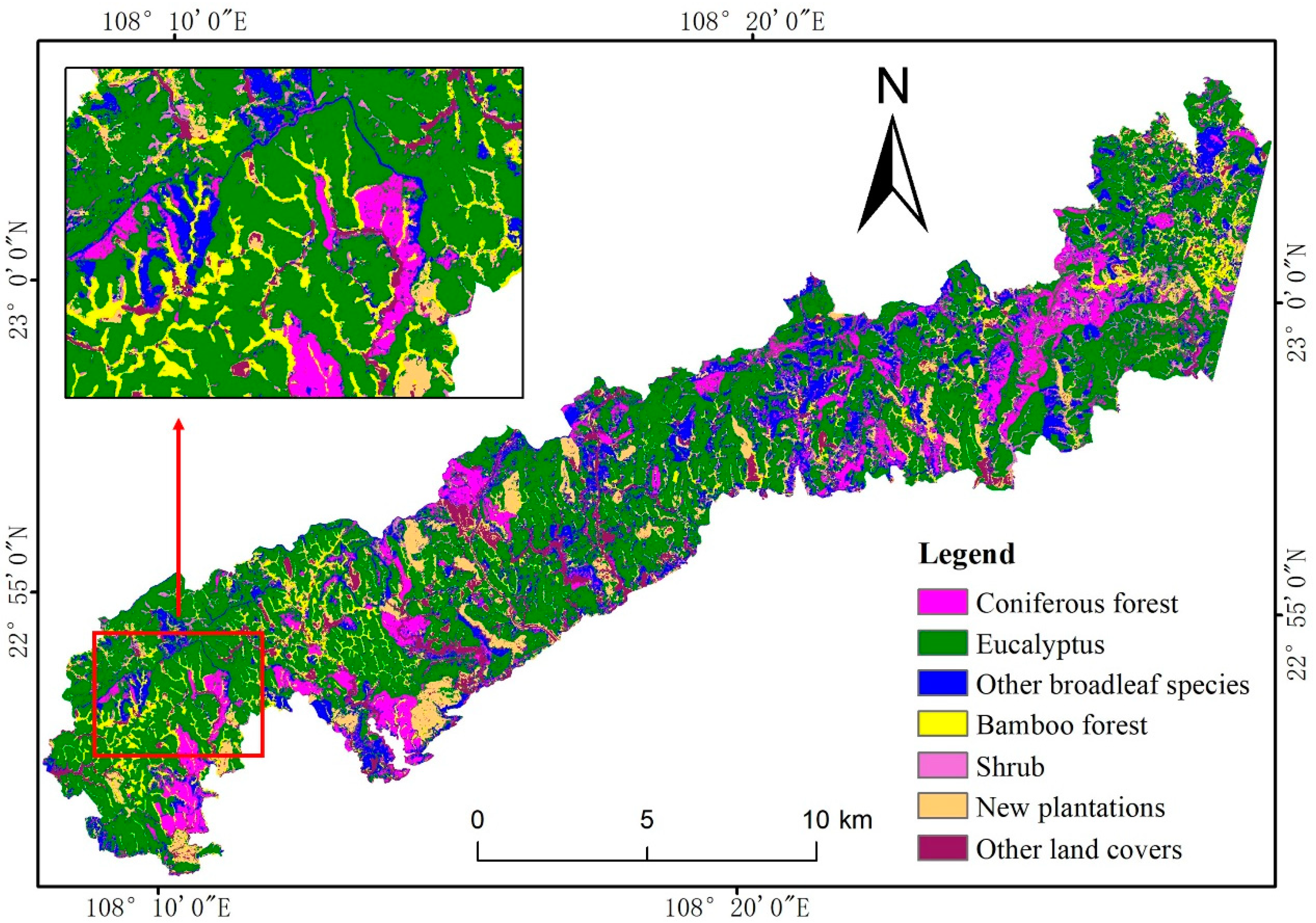
2.1. Study Area

The study area, Gaofeng Forest Farm, is located in northern Nanning City, Guangxi Zhuang Autonomous Region, China (Figure 1). The climate in this region is mild subtropical monsoon with distinct dry and wet seasons with a long summer and short winter. The average annual temperature is about 21 °C and the average annual rainfall is about 1300 mm. This study area has low terrain in the southwest and high terrain in the northeast. The altitude is between 70 m and 900 m and the slope is mainly between 25° and 35°. Gaofeng Forest Farm was established in 1953 and is the largest state-owned forest farm in Guangxi. The total area is about 220 km² with forest coverage of about 85%. The dominant forest types in this farm are plantations, including Masson pine, Chinese fir, eucalyptus, and other broadleaf evergreen forests.

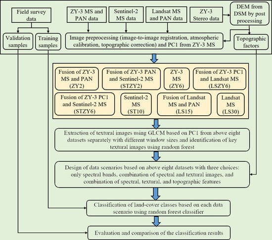
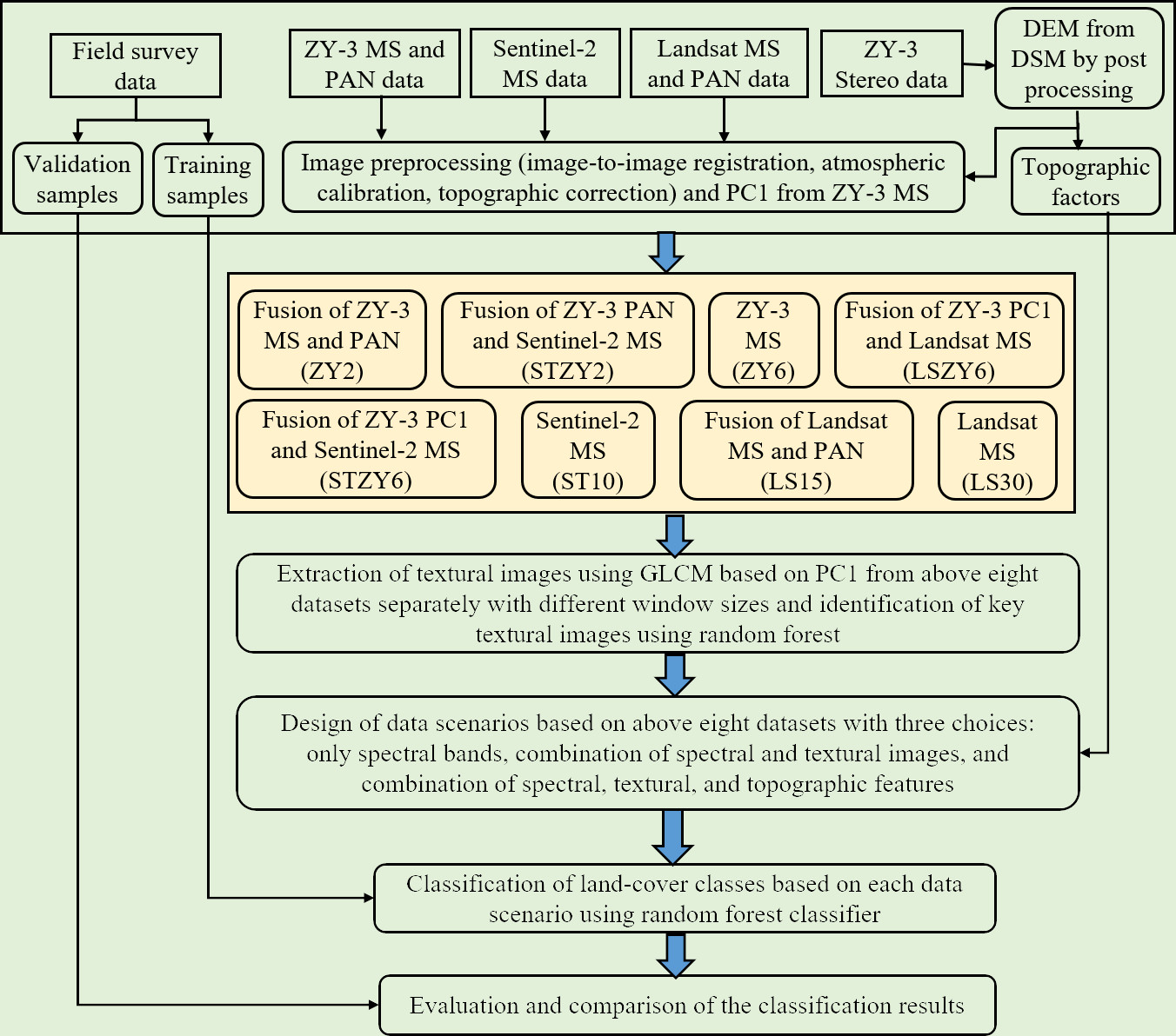
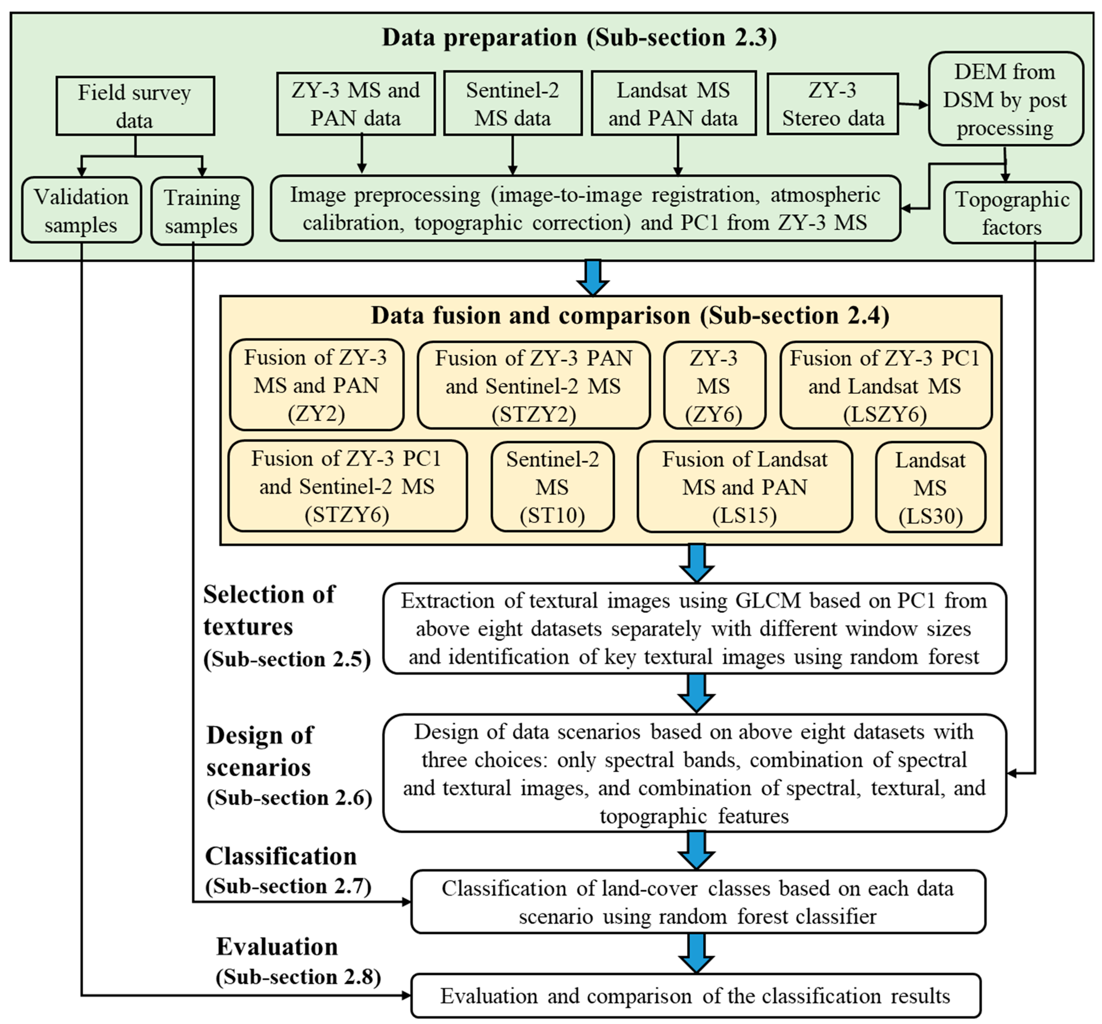
2.2. The Proposed Framework

The strategy of mapping land-cover and forest distribution using different data sources is illustrated in Figure 2. The major steps included the following: (1) Collection and organization of different data sources such as remotely sensed and field survey data. For this study, all remotely sensed data were registered to the Universal Transverse Mercator (UTM) coordinate system and atmospherically and topographically corrected; and all field survey data were organized and randomly selected as training samples or validation samples. (2) Extraction of DEM data from the ZiYuan-3 (ZY-3) stereo image. The resulting DEM data were used for topographic correction of remotely sensed data and for calculation of topographic factors. (3) Data fusion of different spatial resolution images or different optical sensor data. (4) Extraction and selection of textures and design of data scenarios. (5) Implementation of land-cover classification using a random forest (RF) classifier based on different scenarios. (6) Comparison and evaluation of classification results.

2.3. Data Preparations

Datasets used in this research include different optical sensor data (ZY-3, Sentinel-2, and Landsat 8 Operational Land Imager (OLI)), field survey data, and DEM data developed from the ZY-3 stereo data (

Table 1. Datasets used in research.

Dataset	Description	Acquisition Date
ZiYuan–3 (ZY-3) (L1C)	Four multispectral bands (blue, green, red, and near infrared (NIR)) with 5.8-m spatial resolution and stereo imagery (panchromatic band—nadir-view image with 2.1-m, backward and forward views with 3.5-m spatial resolution) were used.	10 March 2018 (Solar zenith angle of 35.68° and solar azimuth angle of 136.74°)
Sentinel-2 (L1C)	Four multispectral bands (three visible bands and one NIR band) with 10-m spatial resolution and six multispectral bands (three red-edge bands, one narrow NIR band, and two SWIR bands) with 20-m spatial resolution were used.	17 December 2017 (Solar zenith angle of 49.37° and solar azimuth angle of 158.68°)
Landsat 8 OLI (L2)	Six multispectral bands (three visible bands, one NIR band, and two SWIR bands) with 30-m spatial resolution and one panchromatic band with 15-m spatial resolution were used.	1 February 2017 (Solar zenith angle of 48.02° and solar azimuth angle of 144.59°)
Field survey	A total of 2166 samples covering different land covers were collected during fieldwork and digitized in the lab.	December 2017 and September 2019
Digital elevation model (DEM)	The DEM data with 2-m spatial resolution were produced from digital surface model (DSM) data which were extracted from the ZY-3 stereo data.	10 March 2018

). All data were registered to the UTM coordinate system.

2.3.1. Collection of Field Survey Data and Design of a Land-Cover Classification System

During field surveys, the coordinates of a site and detailed information about land-cover/forest types, as well as the tree species’ composition, ages of plantation, and estimated height of mixed forest, were recorded for each site visited. All the recorded field data were imported into ArcGIS software and organized in digital format. Field survey data were refined by overlaying the high spatial resolution images from Google Earth and compared with existing forest maps obtained from Farm archives. The refined samples were randomly divided into two groups: Training samples and validation samples. Based on field surveys and our research objectives, a classification system consisting of 11 land-cover classes with special emphasis on forest types (

Table 2. The classification system and samples used in research.

Land-Cover Type	Number of Training Samples	Number of Validation Samples
Masson pine (MP)	168	36
Chinese fir (CF)	118	41
Eucalyptus (EU)	232	194
Chinese anise (CA)	33	33
Castanopsis hystrix (CH)	53	30
Schima (SC)	50	32
Other broadleaf trees (OBT)	37	46
Bamboo forest (BBF)	141	71
Shrub (SH)	105	35
New plantation (NP)	85	42
Other land covers (OLC)	246	88
Total classes: 11	Total training samples: 1268	Total validation samples: 648

Note: Other land covers are mainly nonvegetative, such as bare soils, impervious surfaces, and water.

) was designed.

2.3.2. Collection and Preprocessing of Different Remotely Sensed Data

The remotely sensed data used in this research include ZY-3, Sentinel-2, and Landsat 8 OLI. The ZY-3 multispectral and panchromatic data were orthorectified, then atmospherically calibrated using the fast line-of-sight atmospheric analysis of spectral hypercubes (FLAASH) method, and topographically corrected using SCS+C approach (a modified sun-canopy-sensor topographic correction) [59]. The multispectral images were resampled to a pixel size of 6 m, while the panchromatic band was resampled as 2 m. The ZY-3 imagery was used as reference. Both Sentinel-2 and Landsat 8 OLI images were registered to UTM coordinate system with root mean square error of less than 0.5 pixels. The ZY-3 stereo image was used to develop digital surface model (DSM) data with 2-m spatial resolution [19]. Since DSM represents the land surface height, not bare ground height, it was necessary to conduct post-processing of DSM to reduce the impacts of canopy heights on elevation data [60]. Filtering is a commonly used approach to achieve such a goal. Thus, in this research, a minimum filtering algorithm with a window size of 5 by 5 pixels was first conducted. Then, a median filtering algorithm with the same window size was applied, so the processed DSM could be used as a proxy of DEM for further use in topographic correction of these optical sensor data. The 2-m DEM data were then resampled to 6 m, 10 m, and 30 m using the mean algorithm, matching the cell sizes of satellite images of ZY-3, Sentinel-2, and Landsat OLI, respectively.

The 10 spectral-band Sentinel-2 data (Level-1C product) with 10-m and 20-m spatial resolutions (see Table 1) were used here. The Sentinel-2 Atmospheric Correction (Sen2Cor) was used to conduct atmospheric calibration [61] and Sen2Res was used to convert all spectral bands to the 10-m spatial resolution [62]. For the seven spectral-band Landsat 8 OLI (Level-2 product) data with 30 m for multispectral bands and 15 m for panchromatic band, the LaSRC (Land Surface Reflectance Code) [63] was used for atmospheric calibration. Because the study area is in a mountainous region, undulating terrain has serious impacts on the optical sensor data. It was necessary to conduct topographic correction to reduce the terrain impacts on the surface reflectance values. In this research, the SCS+C approach was used to conduct the topographic correction for both Sentinel-2 and Landsat 8 OLI data, as this algorithm has proven to provide better correction effects, especially when the solar elevation angle is relatively low [59].

2.4. Multisensor/Multiresolution Data Fusion

Many data fusion algorithms are available (see review papers by Pohl and van Genderen [39] and Zhang [40]) and some algorithms such as High Pass Filter (HPF), Gram-Schmidt (GS), and wavelet are often used for data fusion because they can effectively preserve multispectral features while improving spatial details in the fused image [10,19]. HPF extracts rich spatial features from high spatial resolution imagery using a high-pass filtering approach and then adds the extracted features into individual spectral bands [10]. In this research, we used HPF in the following scenarios (note: The following abbreviations ZY, ST, and LS represent ZiYuan-3, Sentinel-2, and Landsat 8 OLI; MS and PAN represent multispectral bands and panchromatic band; PC1 represents the first component from the principal component analysis of the ZY-3 multispectral bands):

(1)

Scenarios at 2-m spatial resolution: (1a) ZY2: Fusion of ZY-3 PAN (2 m) and MS (6 m) data—four multispectral bands with 2-m spatial resolution; (1b) STZY2: Fusion of ZY-3 PAN (2 m) and Sentinel-2 MS (10 m) data—10 multispectral bands with 2-m spatial resolution;

(2)

Scenarios at 6-m spatial resolution: (2a) STZY6: Fusion of ZY-3 PC1 from ZY-3 multispectral image (6 m) and Sentinel-2 MS (10 m) data—10 multispectral bands with 6-m spatial resolution; (2b) LSZY6: Fusion of ZY-3 PC1 from ZY-3 multispectral image (6 m) and Landsat8 OLI MS (30 m) data—six multispectral bands with 6-m spatial resolution;

(3)

Scenarios at 15-m spatial resolution: LS15: Fusion of Landsat PAN (15 m) and MS (30 m) data—six multispectral bands with 15-m spatial resolution.

In addition, the original multispectral bands from ZY6 (ZY-3 MS (6 m)—4 multispectral bands with 6-m spatial resolution), ST10 (Sentinel-2 MS (10 m)—10 multispectral bands with 10-m spatial resolution), and LS30 (Landsat 8 OLI MS (30 m)—6 multispectral bands with 30-m spatial resolution) were also used as comparisons. The PC1 from ZY-3 multispectral image was used here because it concentrates most information from the multispectral bands (over 80% of total variance explained in this research) and only one band with high spatial resolution was required in the HPF data fusion.

2.5. Extraction and Selection of Textural Images

Optical spectral bands may be the most important variables in land-cover classification [35]. As spatial resolution increases, how to effectively incorporate spatial features into spectral data has long been an important research topic [37,64,65]. One approach to use spatial features is to calculate the textural image, a newly generated image from a spectral one, by using a proper texture measure and window size [37]. The GLCM texture measures (mean, variance, homogeneity, contrast, dissimilarity, entropy, second moment, and correlation) are often used in practice due to their easy implementation and effectivity in extracting spatial information [66,67,68]. In order to increase efficiency, we did not conduct the same texture calculation on each spectral band; instead, we conducted principal component analysis on multispectral bands. Then, the PC1 (the first component image) was used for calculation of textural images because the PC1 concentrated the largest amount of information from the multispectral image. Depending on spatial resolution of the images, different window sizes were explored when calculating textural images based on PC1. Specifically, we explored (1) window sizes 5 × 5 to 31 × 31 (14 sizes) at intervals of two for the image at 2-m spatial resolution; (2) window sizes 3 × 3 to 21 × 21 (10 sizes) at intervals of two for the image at 6-m spatial resolution; (3) window sizes 3 × 3 to 15 × 15 (7 sizes) for the images at 10-m and 15-m spatial resolution; and (4) window sizes 3 × 3 to 11 × 11 (6 sizes) for the images at 30-m spatial resolution.

Use of many variables in land-cover classification cannot guarantee a higher classification accuracy [35]. In contrast, using more variables in a classification procedure requires a large number of training samples and demands long processing time and heavy workloads. Because some variables may have limited roles in land-cover classification or some variables have high correlations to each other, identifying the optimal combination of variables becomes necessary before implementing classification [10,33]. One possible solution to identify an optimal combination of variables is the RF algorithm to provide the ranking of variable importance, which is often used in land-cover classification [68,69,70]. Within the selected potential variables using RF, the Pearson’s correlation analysis is used to examine the correlation coefficients between the potential variables. If two variables have high correlation, the one having relatively low-ranking importance may be not needed and, thus, can be removed. This process is repeated until a minimum number of variables is identified while classification performance reaches stability [19]. Therefore, in this research, we used RF to identify the key variables of textural images for each designed dataset. The selected textural images were incorporated into the spectral bands for land-cover classification.

2.6. Design of Data Scenarios

Based on sensor data with various spatial and spectral resolutions (ZY-3, Sentinel-2, and Landsat), as well as topographic factors, different data scenarios were designed for a comparative analysis of classification results to understand how incorporation of textures and topographic factors influence land-cover and forest classification. For each dataset, three data scenarios—spectral bands, combination of spectral and textural images, and combination of spectral bands, textures, and topographic data—were designed. Thus, a total of 24 data scenarios were available, as summarized in

Table 3. Design of data scenarios for land-cover and forest classifications.

Dataset	Data Scenario	Selected Variables
ZY-3 PAN & MS fused data (2 m)	ZY2(4)SP	Blue, Green, Red, NIR
	ZY2(4)SPTX	ZY2(4)SP & (cor_31, cor_9, sec_9, me_31, cor_15, var_13)
	ZY2(4)SPTXTP	ZY2(4)SPTX & (Elevation, Slope, Aspect)
ZY-3 PAN & Sentinel-2 MS fused data (2 m)	STZY2(10)SP	Blue, Green, Red, RedEdge(1–3), NIR, NNIR, SWIR1, SWIR2
	STZY2(10)SPTX	STZY2(10)SP & (cor_31, var_31, cor_9, var_11, sec_5, hom_31)
	STZY2(10)SPTXTP	STZY2(10)SPTX & (Elevation, Slope, Aspect)
ZY-3 MS (6 m)	ZY6(4)SP	Blue, Green, Red, NIR
	ZY6(4)SPTX	ZY6(4)SP & (sec_5, cor_5, cor_7, con_5, hom_21, me_21)
	ZY6(4)SPTXTP	ZY6(4)SPTX & (Elevation, Slope, Aspect)
ZY-3 PC1 and Sentinel-2 MS fused data (6 m)	STZY6(10)SP	Blue, Green, Red, RedEdge(1–3), NIR, NNIR, SWIR1, SWIR2
	STZY6(10)SPTX	STZY6(10)SP & (cor_7, cor_15, cor_5, hom_5, var_5, var_13)
	STZY6(10)SPTXTP	STZY6(10)SPTX & (Elevation, Slope, Aspect)
ZY-3 PC1 and Landsat MS fused data (6 m)	LSZY6(6)SP	Blue, Green, Red, NIR, SWIR1, SWIR2
	LSZY6(6)SPTX	LSZY6(6)SP & (cor_21, cor_7, cor_5, me_21, hom_5, con_5)
	LSZY6(6)SPTXTP	LSZY6(6)SPTX & (Elevation, Slope, Aspect)
Sentinel-2 MS data (10 m)	ST10(10)SP	Blue, Green, Red, RedEdge(1–3), NIR, NNIR, SWIR1, SWIR2
	ST10(10)SPTX	ST10(10)SP & (cor_15, cor_5, cor_9, var_15, hom_15, var_3)
	ST10(10)SPTXTP	ST10(10)SPTX & (Elevation, Slope, Aspect)
Landsat PAN and MS fused data (15 m)	LS15(6)SP	Blue, Green, Red, NIR, SWIR1, SWIR2
	LS15(6)SPTX	LS15(6)SP & (cor_9, me_15, cor_13, cor_5, con_15, cor_3)
	LS15(6)SPTXTP	LS15(6)SPTX & (Elevation, Slope, Aspect)
Landsat MS data (30 m)	LS30(6)SP	Blue, Green, Red, NIR, SWIR1, SWIR2
	LS30(6)SPTX	LS30(6)SP & (me_11, cor_11, con_11, me_3, var_5, cor_7)
	LS30(6)SPTXTP	LS30(6)SPTX & (Elevation, Slope, Aspect)

Note: ZY-3 in dataset column or ZY in data scenario column, ZiYuan-3; ST, Sentinel-2; LS, Landsat 8 OLI (Operational Land Imager); MS, multispectral bands; PAN, panchromatic band; PC1, the first component from the principal component analysis based on ZY-3 multispectral bands; SP, spectral bands; SPTX, spectral bands plus textures; SPTXTP, spectral bands plus textures and topographic factors; 4, 10, 6 in parentheses in data scenario column represent number of spectral bands (spatial resolution).

. The textures in this table were identified using the RF approach based on calculated textural images for each data scenario mentioned before. The DEM-derived elevation, slope, and aspect variables were incorporated into different data scenarios.

2.7. Land-Cover Classification Using the Random Forest Classifier

Selection and optimization of training samples are critical steps in the classification procedure [35]. Based on field surveys, a total of 1268 training samples covering 11 land-cover classes were collected. The number of samples for each land cover is provided in Table 2. Transformed divergence was used to examine the separability of land-cover classes, and optimization of the training samples for each class was conducted through examining spectral curves.

Many classification algorithms, such as maximum likelihood classifier (MLC), artificial neural network (ANN), and support vector machine (SVM), are available [35], but the researcher must select a classification algorithm suitable for a given study area and datasets. The machine learning algorithms such as RF and SVM have been proven to provide better classification than MLC when multisource data are used [11,27,71,72]. Compared with ANN and SVM, which require optimization of different parameters and much longer optimization processing times, RF has the advantages of easy optimization of parameters and much less computation time [71,73]. RF is a nonparametric classifier based on decision tree strategy and has been extensively used for land-cover classification [19,68,69,70]. Three parameters are required to optimize: (1) Ntree, the number of regression trees (default is 500); (2) mtry, the number of input variables per node (default value is one-third of the total variables); and (3) node size (default is one). Node size and mtry are often kept as default values. Thus, the emphasis is on the optimization of ntree. As previous research has indicated, the best ntree value can be 50 [74,75], 100 [68], and even 500 [71] to reach a stable classification accuracy, depending on the classification system and data used. In this research, we explored different ntree values and finally selected 500 as the best value. As summarized in Table 3, RF was used to produce the classification result based on each data scenario. The classification results were then recoded to a system with 11 land-cover classes (see Table 2) for comparative analyses using the accuracy assessment approach.

2.8. Comparative Analysis of Classification Results

A stratification sampling approach with a maximum of 200 samples and minimum of 30 samples was used to collect validation samples. Based on field surveys, all validation samples were visually checked to decide the land-cover type. A total of 648 validation samples were collected and are summarized in Table 2. An error matrix for each scenario was used to evaluate classification results. Overall accuracy and kappa coefficient were calculated from the error matrix [76,77] and used for a comparative analysis of classification results from different scenarios. Meanwhile, user’s accuracy (UA) and producer’s accuracy (PA) were also calculated from each error matrix and used to evaluate the classification accuracy for each land-cover class, especially for individual forest type. In order to easily compare the accuracies among different land-cover types, a mean accuracy (MA) based on PA and UA was calculated; that is, MA = (PA + UA)/2 (Xie et al. 2019). Through comparative analysis of the classification results from different data scenarios, we can better understand the performances of different data sources and whether or not the classification system is suitable for practical applications. In this way, a better forest classification system can be proposed according to research objective and capability of data sources corresponding to given subtropical forest ecosystem.

3. Results

3.1. Comparative Analysis of Classification Results Based on Overall Accuracies

The overall classification results based on different scenarios (

Table 4. A comparison of overall classification accuracies among different data scenarios.

Dataset	Overall Accuracy (%)			Improvement Roles of TX, TP, TXTP (%)			Kappa Coefficient
	SP	SPTX	SPTXTP	TX	TP	TXTP	SP	SPTX	SPTXTP
ZY2(4)	57.87	65.59	69.44	7.72	3.85	11.57	0.50	0.59	0.64
STZY2(10)	72.07	78.09	83.49	6.02	5.40	11.42	0.67	0.74	0.80
Role of Sentinel bands	14.20	12.50	14.05				0.17	0.15	0.16
ZY6(4)	62.44	68.78	74.19	6.34	5.41	11.75	0.56	0.63	0.69
STZY6(10)	73.57	76.20	77.43	2.63	1.23	3.86	0.69	0.71	0.73
LSZY6(6)	66.15	68.93	71.72	2.78	2.79	5.57	0.60	0.63	0.67
Role of Sentinel bands	11.13	7.42	3.24				0.13	0.08	0.04
Role of Landsat bands	3.71	0.15	−2.47				0.04	0	−0.02
ST10(10)	68.21	69.44	73.77	1.23	4.33	5.56	0.63	0.64	0.69
LS15(6)	61.80	63.51	68.99	1.71	5.48	7.19	0.55	0.57	0.64
LS30(6)	59.88	60.96	65.99	1.08	5.03	6.11	0.54	0.55	0.60

Note: The abbreviations in this table are given in Table 2 and Table 3.

) indicate that the STZY2(10) under SPTXTP (combination of spectral bands, textures, and topographic factors) provided the best classification with overall accuracy of 83.5% and kappa coefficient of 0.80, followed by STZY2(10) under SPTX (combination of spectral bands and textures) and STZY6(10) under SPTX or SPTXTP with overall accuracies of 76.2–78.1% and kappa coefficients of 0.71–0.74. All other scenarios had overall accuracies of less than 74.2% and kappa coefficient of less than 0.69. These results imply the important roles of both spectral and spatial resolutions through fusion of ZY-3 and Sentinel-2 data and the importance of incorporating textural images and topographic factors into spectral bands. The comprehensive role of both textures and topographic factors in 2-m spatial resolution images improved overall accuracy by 11.4–11.6% compared with only spectral bands.

3.1.1. The Role of Spectral Features in Land-Cover Classification

Considering the classification results using spectral bands only, STZY6(10) provided the best accuracy of 73.6%, followed by STZY2(10) with 72.1%, while ZY2(4) provided the poorest accuracy of 57.9%, following LS30(6) with 59.9%, implying the importance of combined spectral and spatial features in improving land-cover classification. Overall, 10 spectral bands (STZY2(10), STZY6(10), ST10(10)) had better classification accuracy (68.2–73.6%) than six bands (59.9–66.2%) and four bands (57.9–62.4%), implying the important role of an increased number of spectral bands in improving land-cover classification. For example, at 2-m spatial resolution, the increasing number of spectral bands from 4 (ZY2(4)) to 10 (STZY2(10)) improved classification accuracy by 14.2%; at 6-m spatial resolution and the same increase in spectral bands from ZY6(4) to STZY6(10), the overall accuracy increased by 11.1%, but increasing the spectral bands from four (ZY6(4) to six (LSZY6(6)) increased the overall accuracy by only 3.7%, implying the important roles of using red-edge and narrow NIR bands (only in Sentinel-2) in addition to the SWIR bands (in both Sentinel-2 and Landsat OLI).

The role of data fusion varies in improving land-cover classification, depending on the number of spectral bands and spatial resolution. If the spatial resolution is the same, increasing the number of spectral bands can considerably improve classification accuracy, for example, from ZY2(4) to STZY2(10) and from ZY6(4) to LSZY6(6) or STZY6(10). However, if the number of spectral bands is the same, the role of improved spatial resolution varies; for instance, higher spatial resolution may produce higher heterogeneity of the same forest class, resulting in reduced classification accuracy, as shown in the data scenarios between ZY6(4) and ZY2(4), and between STZY6(10) and STZY2(10). However, for the relatively coarse spatial resolution images, improved spatial resolution is indeed helpful for land-cover classification, as shown in the data scenarios among LS30(6), LS15(6), and LSZY6(6), and between ST10(10) and STZY6(10). These results imply that a high spatial resolution image without a sufficient number of spectral bands (e.g., ZY2(4)) or a relatively coarse spatial resolution image (LS30(6)) provides poor classification accuracy (less than 60% in this research), while the imagery having both high spatial and spectral resolutions (e.g., STZY6(10)) provides the best classification accuracy, implying the importance of selecting remotely sensed data with both spectral and spatial resolutions suitable for land-cover classification.

3.1.2. The Role of Textures in Land-Cover Classification

For the data scenarios under SPTX, STZY2(10) and STZY6(10) provided the best accuracies, of 78.1% and 76.2%, followed by ST10(10), LSZY6(6), and ZY(6) with overall accuracies of 68.8–69.4%, and LS30 had the poorest accuracy at only 61%, implying different roles of textures in improving land-cover classification. One important finding in Table 4 is that incorporation of textures into spectral bands improved land-cover classification, but the contribution of textures varied, depending on spatial resolution and the number of spectral bands. As shown in Table 4, using textures in ZY6(4) and ZY2(4) improved overall accuracy by 6.3% and 7.7%, respectively, in ST10(10), STZY6(10), and STZY2(10) by 1.2%, 2.6%, and 6.0%, respectively, and in LS30(6), LS15(6), and LSZY6(6) by 1.1%, 1.7%, and 2.8%, respectively. For the same number of spectral bands, the textures from higher spatial resolution imagery (better than 6 m) played more important roles than the ones from relatively coarse spatial resolution imagery. This finding indicates the need to combine the spatial features from high spatial resolution imagery into spectral bands to produce accurate land-cover classification.

3.1.3. The Role of Topographic Factors in Land-Cover Classification

Incorporation of topographic factors into spectral and textural datasets—SPTXTP—improved overall accuracy by 1.2–5.5% for all scenarios. The highly improved accuracies of 5.0–5.5% were from STZY2(10), ZY6(4), LS15(6), and LS30(6) scenarios, implying the complex roles of topographic factors in land-cover classification. The topographic factors had relatively low effects (increased accuracy by only 1.2–2.8%) on the data scenarios such as STZY6(10) and LSZY6(6) with 6-m spatial resolution and 10 or six spectral bands. The results in Table 4 indicate that the role of topographic factors is more important in high spatial resolution images (better than 6 m) or relatively low spatial resolution images (15 or 30 m here) than the 6-m spatial resolution images with more spectral bands.

3.1.4. The Comprehensive Roles of Textures and Topographic Factors in Land-Cover Classification

Compared to spectral bands alone (SP data scenario), incorporation of both textures and topography into spectral data improved overall land-cover classification accuracies by 3.9–11.8%. In particular, the data scenarios with high spatial resolution such as ZY2(4), ZY2(10), and ZY6(4) improved overall accuracies by 11.4–11.8%. Generally speaking, textures played more important roles than topography for high spatial resolution images but inversely for relatively coarse spatial resolution images. The least improvement using both textures and topography occurred in STZY6(10) with increased accuracy of only 3.9%. This situation implies that the combined effects of both textures and topographic factors relied on the spectral and spatial resolutions.

3.2. Comparative Analysis of Classification Results Based on Individual Forest Classes

The mean accuracies of individual land-cover classes (

Table 5. A comparison of mean accuracies of individual classes among scenarios from ZY-3 and Sentinel-2.

Data Scenarios		Classification Accuracies (%) for Individual Classes
		MP	CF	EU	CA	CH	SC	OBT	BBF	SH	NP	OLC
ZY2(4)	SP	46.38	52.17	72.48	41.80	13.81	74.78	33.60	33.94	60.33	55.03	83.64
	SPTX	49.92	58.43	76.97	59.53	40.00	80.59	35.87	42.42	68.57	66.72	88.14
	SPTXTP	53.24	65.21	80.49	64.94	51.58	78.75	41.22	50.02	68.89	68.29	89.27
Role of TX, TP, TXTP	TX	3.54	6.26	4.49	17.73	26.19	5.81	2.27	8.48	8.24	11.69	4.50
	TP	3.32	6.78	3.52	5.41	11.58	−1.84	5.35	7.60	0.32	1.57	1.13
	TXTP	6.86	13.04	8.01	23.14	37.77	3.97	7.62	16.08	8.56	13.26	5.63
STZY2(10)	SP	50.93	49.07	83.12	68.68	56.67	80.36	43.68	78.29	62.82	71.33	88.30
	SPTX	64.05	62.85	85.62	71.66	58.67	78.88	59.85	80.22	66.92	86.54	94.39
	SPTXTP	66.65	69.36	90.13	70.65	64.76	87.06	76.49	91.08	73.74	89.01	94.39
Role of TX, TP, TXTP	TX	13.12	13.78	2.50	2.98	2.00	−1.48	16.17	1.93	4.10	15.21	6.09
	TP	2.60	6.51	4.51	−1.01	6.09	8.18	16.64	10.86	6.82	2.47	0.00
	TXTP	15.72	20.29	7.01	1.97	8.09	6.70	32.81	12.79	10.92	17.68	6.09
ZY6(4)	SP	54.50	60.91	74.63	58.34	33.05	85.27	29.60	46.70	51.43	61.98	84.93
	SPTX	63.30	65.15	78.27	64.79	48.89	77.09	47.56	48.48	68.10	67.74	88.64
	SPTXTP	66.67	70.65	82.45	64.64	52.78	83.26	66.58	69.84	66.92	68.39	88.14
Role of TX, TP, TXTP	TX	8.80	4.24	3.64	6.45	15.84	−8.18	17.96	1.78	16.67	5.76	3.71
	TP	3.37	5.50	4.18	−0.15	3.89	6.17	19.02	21.36	−1.18	0.65	−0.50
	TXTP	12.17	9.74	7.82	6.30	19.73	−2.01	36.98	23.14	15.49	6.41	3.21
STZY6(10)	SP	54.39	59.19	85.63	70.00	66.67	75.43	48.34	73.47	66.92	68.75	87.73
	SPTX	57.45	67.98	84.21	79.08	62.23	76.21	52.37	78.42	68.89	77.43	92.05
	SPTXTP	59.63	61.43	85.45	72.21	71.88	80.65	58.97	84.13	70.72	78.86	91.97
Role of TX, TP, TXTP	TX	3.06	8.79	−1.42	9.08	−4.44	0.78	4.03	4.95	1.97	8.68	4.32
	TP	2.18	−6.55	1.24	−6.87	9.65	4.44	6.60	5.71	1.83	1.43	−0.08
	TXTP	5.24	2.24	−0.18	2.21	5.21	5.22	10.63	10.66	3.80	10.11	4.24
ST10(10)	SP	50.60	58.93	78.72	71.97	72.97	49.45	54.35	73.30	55.09	72.86	88.91
	SPTX	53.65	59.49	77.58	66.41	64.62	53.37	55.44	77.49	60.88	75.58	90.75
	SPTXTP	57.87	65.14	80.40	68.38	65.29	71.58	59.20	80.22	60.88	76.82	89.67
Role of TX, TP, TXTP	TX	3.05	0.56	−1.14	−5.56	−8.35	3.92	1.09	4.19	5.79	2.72	1.84
	TP	4.22	5.65	2.82	1.97	0.67	18.21	3.76	2.73	0.00	1.24	−1.08
	TXTP	7.27	6.21	1.68	−3.59	−7.68	22.13	4.85	6.92	5.79	3.96	0.76

Note: The abbreviations in this table are given in Table 2 and Table 3.

and

Table 6. A comparison of mean accuracies of individual classes among scenarios from ZY-3 and Landsat.

Data Scenarios		Classification Accuracies (%) for Individual Classes
		MP	CF	EU	CA	CH	SC	OBT	BBF	SH	NP	OLC
ZY6(4)	SP	54.50	60.91	74.63	58.34	33.05	85.27	29.60	46.70	51.43	61.98	84.93
	SPTX	63.30	65.15	78.27	64.79	48.89	77.09	47.56	48.48	68.10	67.74	88.64
	SPTXTP	66.67	70.65	82.45	64.64	52.78	83.26	66.58	69.84	66.92	68.39	88.14
Role of TX, TP, TXTP	TX	8.80	4.24	3.64	6.45	15.84	−8.18	17.96	1.78	16.67	5.76	3.71
	TP	3.37	5.50	4.18	−0.15	3.89	6.17	19.02	21.36	−1.18	0.65	−0.50
	TXTP	12.17	9.74	7.82	6.30	19.73	−2.01	36.98	23.14	15.49	6.41	3.21
LSZY6(6)	SP	42.77	59.97	80.82	64.64	70.00	72.38	18.64	59.91	50.90	65.68	80.27
	SPTX	46.18	62.28	81.93	61.56	73.34	74.44	42.03	67.56	47.86	66.34	81.50
	SPTXTP	52.13	65.07	83.11	70.00	70.37	76.48	44.40	75.83	52.99	67.74	82.23
Role of TX, TP, TXTP	TX	3.41	2.31	1.11	−3.08	3.34	2.06	23.39	7.65	−3.04	0.66	1.23
	TP	5.95	2.79	1.18	8.44	−2.97	2.04	2.37	8.27	5.13	1.40	0.73
	TXTP	9.36	5.10	2.29	5.36	0.37	4.10	25.76	15.92	2.09	2.06	1.96
LS15(6)	SP	43.67	42.50	77.19	59.42	63.95	45.05	17.69	60.32	56.98	64.76	84.17
	SPTX	43.41	50.64	77.37	66.41	62.37	59.67	30.44	55.35	56.84	61.38	83.64
	SPTXTP	51.44	58.24	80.87	72.62	72.50	61.82	44.21	65.81	52.49	69.05	84.58
Role of TX, TP, TXTP	TX	−0.26	8.14	0.18	6.99	−1.58	14.62	12.75	−4.97	−0.14	−3.38	−0.53
	TP	8.03	7.60	3.50	6.21	10.13	2.15	13.77	10.46	−4.35	7.67	0.94
	TXTP	7.77	15.74	3.68	13.20	8.55	16.77	26.52	5.49	−4.49	4.29	0.41
LS30(6)	SP	45.33	41.62	75.39	66.79	56.73	50.70	33.94	62.66	39.54	59.75	80.77
	SPTX	46.30	57.50	74.68	68.77	66.27	53.49	33.34	59.31	37.14	59.53	80.10
	SPTXTP	43.75	59.66	77.93	70.00	57.22	54.77	54.79	67.78	45.72	68.23	84.17
Role of TX, TP, TXTP	TX	0.97	15.88	−0.71	1.98	9.54	2.79	−0.60	−3.35	−2.40	−0.22	−0.67
	TP	−2.55	2.16	3.25	1.23	−9.05	1.28	21.45	8.47	8.58	8.70	4.07
	TXTP	−1.58	18.04	2.54	3.21	0.49	4.07	20.85	5.12	6.18	8.48	3.40

Note: The abbreviations in this table are given in Table 2 and Table 3.

) indicate that different data sources have their own performances in classifying individual classes. Spectral features are still the most important for land-cover classification, and incorporation of textures and topographic factors improved some land-cover classes. Overall, eucalyptus had high classification accuracies of 72.5–90.1%, no matter which datasets were used. In particular, STZY2(10) and STZY6(10) provided the best accuracies of 83.1–90.1% and 84.2–85.6%, respectively, for eucalyptus, implying the importance of both spatial and spectral features. The following subsections will mainly focus on the accuracy analysis based on forest types.

3.2.1. The Role of Spectral Features in Individual Forest Classification

Although spectral signature is the most important feature in forest classification, its role varies depending on specific forest types. For example, at 2-m spatial resolution, four spectral bands with three visible bands and one NIR band (ZY2(4)) cannot effectively separate forest classes, but the 10 spectral bands with visible, red-edge, NIR, and SWIR bands (STZY2(10)) can considerably improve classification accuracy. For example, Table 5 and Table 6 show that the classification accuracy for Castanopsis hystrix can increase from 13.8% to 56.7%, and bamboo forest from 33.9% to 78.3%. Overall, no matter which data source was used, eucalyptus had the best accuracies, of 72.5–85.6%, but Masson pine, Chinese fir, and other broadleaf trees had accuracies of less than 54.5%, 60.9%, and 54.4%, respectively. Other forest types had various accuracy ranges, depending on which kinds of data sources were used.

With the same spatial resolution, an increased number of spectral bands improved classification accuracies for the majority of forest types; for example, STZY2(10) provided much better classification accuracies for eucalyptus, Chinese anise, Castanopsis hystrix, Schima, and bamboo forest than ZY2(4). A similar situation occurred with ZY6(4), LSZY6(6), and STZY6(10) for eucalyptus, Chinese anise, and bamboo forest, but not for Masson pine or Chinese fir. In contrast, for the same number of spectral bands, increased spatial resolution (e.g., ZY2(4) vs. ZY6(4)) did not improve forest classification accuracy and made it worse for most forest types. This may be due to the high spatial resolution resulting in high spatial heterogeneity in images. For the 10 spectral bands, STZY6(10) provided the best accuracies for Masson pine, Chinese fir, and eucalyptus, but STZY2(10) provided the best for Schima and bamboo forest, while ST10(10) provided the best for Chinese anise, Castanopsis hystrix, and other broadleaf trees, implying that spatial resolution may play important roles for forest classification but different forest types require different spatial resolutions because of their unique forest canopy structures. Considering six spectral bands with spatial resolutions from 6 m to 15 m to 30 m, LSZY6 provided the best classification accuracies for Chinse fir, eucalyptus, Castanopsis hystrix, and Schima, but LS30 provided the best for Masson pine and Chinese anise. Overall, spectral signatures alone cannot provide high classification accuracy for most forest types, and 6 m, instead of 2 m or coarser than 10 m, is the optimal spatial resolution. This implies that proper selection of spatial and spectral resolutions is needed for forest classification. Individual sensor data do not have both high spatial and high spectral resolutions and, thus, data fusion is an alternative to improve both spatial and spectral features, thus improving forest classification, as shown in Table 5 and Table 6.

3.2.2. The Role of Textures in Individual Forest Classification

Spectral bands alone, especially without NIR and SWIR bands, make it difficult to extract some forest types such as Masson pine, Chinese anise, Castanopsis hystrix, other broadleaf trees, and bamboo forest, but incorporation of textures considerably improved their classification accuracies. However, the effectiveness of using textural images is influenced by spatial resolution. As shown in Table 5 and Table 6, the textures from STZY2(10) provided the best accuracies for Masson pine, eucalyptus, other broadleaf trees, and bamboo forest. The textures from STZY6(10) worked best for Chinese fir and Chinese anise. The textures from ZY2(4) worked best for Schima and the textures from LSZY6(6) worked best for Castanopsis hystrix, implying that textures from high spatial resolution images played more important roles than those from medium spatial resolution images in improving forest classification.

For ZY2(4) with 2-m spatial resolution, incorporation of textures into spectral bands improved classification accuracies for all forest types. In particular, the accuracies for Chinese anise and Castanopsis hystrix, respectively, increased from 41.8% and 13.8% based on spectral bands alone to 59.3% and 40.0% on the combination of spectral and textural images. For relatively coarse spatial resolution data, such as LS15(6) and LS30(6), incorporation of textural images into spectral bands yielded some improvement for forest types such as Chinese fir, Chinese anise, and Schima, but may have worse accuracies for other forest types such as Masson pine, eucalyptus, and bamboo forest. For 6-m spatial resolution, incorporation of textural images into spectral bands improved classification accuracy for most forest types. The results in Table 5 and Table 6 imply the need to identify suitable textures that correspond to specific forest types, and no textures are optimal for different forest types because of their differences in forest stand structures, patch sizes, and shapes.

3.2.3. The Role of Topographic Features in Individual Forest Classification

The roles of topographic factors depend on specific forest types and spatial and spectral resolutions of datasets used. Overall, the incorporation of topographic factors into spectral and textural images improved classification accuracies of most forest types; the improvement was as high as 18.2% for Schima in ST10(10)) and 19.0% and 21.5% for other broadleaf trees in ZY6(4) and LS30(6), respectively. However, these forest types had relatively low accuracies based on the combination of spectral and textural images. In some cases, for example, use of topographic factors in STZY6(10) reduced classification accuracies for Chinese fir and Chinese anise by 6.6% and 8.9%, respectively. This situation implies that use of topographic factors as extra bands should consider the sensitivity of topography on forest distribution.

3.2.4. The Comprehensive Roles of Textures and Topographic Factors in Individual Forest Classification

Overall, STZY2(10)_SPTXTP provided the best classification accuracies for most forest types in this study (Table 5 and Table 6): The accuracies for eucalyptus, bamboo forest, and Schima reached 90.1%, 91.1%, and 87.1%, respectively, while Masson pine, Chinese fir, and other broadleaf trees had their best accuracies of 66.7–76.5%, implying that the incorporation of spectral bands, textural images, and topographic factors based on high spectral and spatial resolutions is needed for forest classification. On the other hand, the best classification accuracy for Chinese anise was 79.1% with STZY6(10) and the best accuracy for Castanopsis hystrix was 73.3% with LSZY6(6) under SPTX scenario, implying the important roles of both spectral bands and textures in forest classification, but topographic factors may be not needed for some forest classification. Table 5 and Table 6 show the difficulty of classification for some forest types and the need to design a proper forest classification that takes the classification accuracies, research objectives, and complexity of forest ecosystem into account.

3.2.5. Design of Different Forest Classification Systems

The classification results in Table 4 show that the data scenario STZY2(10)_SPTXTP provided the best classification accuracy of 83.5%. However, Table 5 and Table 6 indicate that some forest types, such as Castanopsis hystrix, Masson pine, and Chinese fir, had relatively low accuracies of 64.8–69.4%. As shown in

Table 7. A comparison of individual classification accuracies between two classification systems.

	Classification Accuracies of Individual Classes											OA	KA
	MP	CF	EU	CA	CH	SC	OBT	BBF	SH	NP	OLC
PA	80.56	51.22	94.33	72.73	53.33	81.25	73.91	92.96	62.86	85.71	95.45	83.49	0.80
UA	52.73	87.50	85.92	68.57	76.19	92.86	79.07	89.19	84.62	92.31	93.33
MA	66.65	69.36	90.13	70.65	64.76	87.06	76.49	91.08	73.74	89.01	94.39
	CFF		EU	OBS				BBF	SH	NP	OLC	OA	KA
PA	92.21		94.33	80.85				92.96	62.86	85.71	95.45	88.89	0.86
UA	89.87		85.92	89.76				89.19	84.62	92.31	93.33
MA	91.04		90.12	85.31				91.07	73.74	89.01	94.39

Note: PA, UA, and MA represent producer’s accuracy, user’s accuracy, and mean accuracy, respectively, of an individual class [i.e., MA = (PA + UA)/2]; OA, overall accuracy; KA, kappa coefficient; meanings of the land-cover abbreviations used in this table are given in Table 2.

, Chinese fir and Castanopsis hystrix had PAs of 51.2% and 53.3%, respectively, and Masson pine had a UA of 52.7%, implying major confusion among some forest types. For example, the error matrix from the STZY2(10)_SPTXTP classification result (

Table 8. Error matrix based on the best accuracy result from the STZY2(10)_SPTXTP data scenario.

	Reference Data											Row Total	UA	PA
	MP	CF	EU	CA	CH	SC	OBT	BBF	SH	NP	OLC
MP	29	18	2	3	1	1	0	0	0	0	1	55	52.73	80.56
CF	3	21	0	0	0	0	0	0	0	0	0	24	87.50	51.22
EU	1	1	183	4	6	2	8	2	6	0	0	213	85.92	94.33
CA	2	0	0	24	6	0	2	0	1	0	0	35	68.57	72.73
CH	0	0	4	0	16	0	1	0	0	0	0	21	76.19	53.33
SC	0	1	0	0	0	26	0	0	0	0	1	28	92.86	81.25
OBT	1	0	1	1	1	3	34	1	1	0	0	43	79.07	73.91
BBF	0	0	3	0	0	0	1	66	4	0	0	74	89.19	92.96
SH	0	0	1	1	0	0	0	2	22	0	0	26	84.62	62.86
NP	0	0	0	0	0	0	0	0	1	36	2	39	92.31	85.71
OLC	0	0	0	0	0	0	0	0	0	6	84	90	93.33	95.45
Total	36	41	194	33	30	32	46	71	35	42	88

Note: The meanings of the land-cover abbreviations used in this table are given in Table 2.

) shows that Masson pine is highly confused with Chinese fir, and Chinese anise is confused with Castanopsis hystrix. This result indicates that current classifications cannot provide sufficiently high accuracy for some forest types, and it is necessary to design a proper classification system by combining research objectives, remotely sensed data, and classification procedure so the accuracy for each type can meet the user’s requirement for real applications.

Based on data scenarios currently used, some forest types have relatively low classification accuracies that are not suitable for real applications such as forest management. Considering that Masson pine and Chinese fir belong to coniferous forest, they can be grouped into that class, while Chinese anise, Castanopsis hystrix, Schima, and other broadleaf trees, which constitute a small proportion of this study area, can be grouped into one class called other broadleaf species (except eucalyptus). The newly merged classes—coniferous forest and other broadleaf species—had average accuracies of 91.0% and 85.3%, respectively. Overall accuracy and kappa coefficient of seven classes became 88.9% and 0.86, respectively, and mean accuracies of forest classes reached 85.3–91.1% (see Table 7). As an example of the classification image with seven land-cover classes, Figure 3 shows that eucalyptus plantations were distributed throughout the study area and made up the largest proportion, followed by coniferous forest. Other broadleaf forests and bamboo forests had small proportions and were widely dispersed.

4. Discussion

4.1. Increasing the Number of Spectral Bands to Improve Land-Cover and Forest Classification

Spectral signature is fundamental for land-cover and forest classification, and multispectral imagery is commonly used but cannot produce sufficiently high classification accuracies for all classes [19,20]. This is especially true when high spatial resolution images with only a limited number of spectral bands (visible and NIR) are used. Considering complex forest landscapes with various patch sizes, this research exhibited the importance of using both high spatial and spectral resolution images. However, in fact, the majority of high spatial resolution optical sensor images such as Quickbird, IKONOS, ZY-3, and GaoFen-1 have only four spectral bands consisting of visible and NIR bands. The fewer spectral bands limit their capability of differentiating forest types and species, especially in subtropical regions with rich tree species, due to the spectral confusion of some forest types and impacts of undulating terrain on surface reflectance values. This research indicated the importance of inclusion of more spectral bands such as red-edge and SWIR into the classification procedure. On the other hand, Landsat images with relatively coarse spatial resolution are not sufficient for implementing fine forest classification in a complex forest ecosystem with relatively small patch sizes due to the mixed pixel problem. To overcome this problem, data fusion is an effective tool to integrate high spatial and spectral features into a new dataset. This research used HPF to conduct the fusion of different sensor data (e.g., ZY-3 PAN and Sentinel-2 MS) or different spatial resolution images from the same sensor data (e.g., ZY-3 MS and PAN, Landsat 8 OLI MS and PAN) and found that the fused images indeed improved classification accuracy, a conclusion similar to tropical forest classification research in the Brazilian Amazon [10,27,33].

Another way to increase the number of spectral bands is to use multitemporal images. Use of images from different seasons is especially valuable for distinguishing deciduous and evergreen vegetation classes [11,19,45]. However, in subtropical regions where evergreen forests dominate, multitemporal images may not provide much new information for distinguishing forest classes, and cloud-free images are somewhat rare. An alternative is to use hyperspectral images such as Hyperion or airborne hyperspectral images [78,79,80]. However, hyperspectral imagery has not been used extensively for forest classification due to the difficulty of image acquisition for a given study area. Therefore, more research may be focused on making full use of multisource data such as spatial features inherent in the spectral signatures and ancillary data in a classification procedure.

4.2. Incorporating Textures into Spectral Data to Improve Land-Cover and Forest Classification

This research showed that incorporation of textures into spectral bands can considerably improve overall classification accuracies (see Table 4), especially when high spatial resolution images are used. Many previous studies also came to this conclusion [10,33,37]. The roles of textures in improving specific forest classes vary, depending on spatial and spectral features. This implies the difficulty in identifying universal textures that can be used to improve classification accuracy for each class. One key in using textural images is to identify an optimal combination of textural images. This involves deciding how many textural images should be selected. Some previous studies focusing on vegetation classification indicated that incorporation of two or three textural images as extra bands into spectral data is suitable, based on separability analysis of training samples [37]. There are so many potential scenarios of different combinations, it is often difficult to identify an optimal one. This research used RF to identify the best combination of textural images based on an importance ranking and has proven to be an effective method.

The important role of textures in improving forest classification is well recognized, but lack of universal knowledge to guide the selection of textures in a study area hinders the process. Selection of a suitable window size for calculation of textural images is critical and depends on the spatial resolution of the image and complexity of forest landscapes under investigation [37]. Window sizes 7 × 7 and 9 × 9 pixels were found to be suitable for calculation of textures from Landsat images [10]. As spatial resolution increases, such as with Quickbird, the window size can be as large as 21 × 21 pixels [81]. This research indicated that a large window size such as 31 × 31 or 25 × 25 is needed for high spatial resolution images (2 m), and a small window size such as 5 × 5 is needed for medium spatial resolution images (30 m). Also, a combination of textural images from different window sizes and texture measures is necessary but may not improve the accuracies for some forest types. Therefore, more research should be conducted on the selection of suitable textures for specific forest classes, not based on overall land covers.

4.3. Using Ancillary Data to Improve Land-Cover and Forest Classification

Ancillary data such as population density, DEM, and soil type are easily obtainable and may be used in a land-cover or forest classification. How to effectively employ ancillary data to improve land-cover classification has long been an important research topic [35]. In mountainous regions, spatial distribution of different land-cover or forest types is often related to topography and soil types. For example, agricultural lands and villages are usually located in relatively flat areas, and some tree species are likely to appear in sunny- or shady-slope areas. Previous studies have explored the effectiveness of employing topographic factors to improve forest classification [19]. This research confirmed their important roles in improving forest classification. In addition, we found that topographic factors have different effects in differentiation of forest types. As shown in Table 5 and Table 6, topographic factors can improve classification accuracies of Masson pine, Chinese fir, and eucalyptus for different data scenarios, but may reduce accuracies for Chinese anise based on data scenarios such as STZY2(10), ZY6(4), and STZY6(10), implying the different roles of topographic factors in distinguishing forest types. It also implies that direct use of topographic factors as extra variables may not be an optimal method. Suitable expert knowledge must be developed about the relationships between topographic factors and specific forest distribution to enhance forest classification. With such knowledge, the hierarchically based approach that can effectively determine specific variables for extraction of forest types may be preferable [20].

4.4. The Importance of Using Multiple Data Sources to Improve Land-Cover and Forest Classification

Single-sensor remotely sensed data have limitations in spectral and spatial features and, thus, may not produce accurate land-cover classification, especially for forest types in subtropical regions under complex terrain conditions and rich tree species. This research confirmed that proper integration of different data sources, such as spectral bands, textural images, and topographic factors, can considerably improve forest classification. However, it is necessary to consider the spatial and spectral resolutions when different data sources are combined, because the ability to improve classification performance may be vastly different. Considering the forest types, differences in forest stand structures among forest types, especially plantations such as eucalyptus in this research, are important features that can be used. Texture is one of the features that can reflect different forest stand structures. Previous research has indicated that proper use of spectral mixture analysis on the Landsat multispectral imagery can improve forest classification [10,82]. With Lidar and stereo imagery, the canopy features from those images may be an alternative to incorporate into optical sensor data to improve forest classification [83,84,85]. More research is needed to explore how to effectively integrate different data sources in a classification procedure and what classification algorithm is optimal for a forest classification based on multiple data sources.

In tropical and subtropical regions, cloud is often a problem for collection of cloud-free optical sensor data. Thus, different sensor data with various acquisition dates have to be used in reality. In this case, cautions should be taken to reduce the effects of different acquisition dates of data in land-cover classification. As shown in Table 1, we used ZY-3 imagery on 10 March 2018 and Landsat OLI imagery on 1 February 2017. The one-year gap between both images may influence the data fusion result because the fast growth of some tree species such as eucalyptus in this research may affect the tree crown size and forest canopy density, thus affecting forest reflectance in the optical sensor data. This difference caused by the gap of image acquisition dates may affect forest classification results. Therefore, we paid much attention to the selection of training samples and validation samples to avoid the potential impacts of land-cover change (e.g., eucalyptus harvest) on the classification and accuracy assessment.

In addition to the careful selection of suitable input variables from different data sources (e.g., remotely sensed data, ancillary data), collection of sufficient number of training samples and validation samples for each class is also critical for a successful land-cover classification. In general, samples are often collected from field survey or visual interpretation of high spatial resolution images based on Google Earth. Considering the expense and intensive labor when doing field work, effective use of existing open data sources will be an alternative to collect more samples. The crowdsourced data such as OpenStreetMap and Volunteered Geographic Information obtained through Citizen Science may be used for collection of training and validation samples [86,87]. This is especially important when multiple source data are used as input variables for land-cover and forest classification using advanced machine learning algorithms such as deep learning [15,85,88]. More research is needed to design an optimal procedure to include multiple data sources as input variables for classification and to select useful samples from open data sources in addition to the field survey data.

5. Conclusions

This research explored land-cover classification with emphasis on forest types in a subtropical region through a comprehensive comparison of classification results based on multiple data sources (i.e., ZY-3, Snetinel-2, and Landsat 8 OLI). Data scenarios based on spectral, textural, and topographic data with spatial resolution ranges from 2 m to 30 m were designed, and RF was used to conduct the classification. Major conclusions are summarized as follows:

(1)

Spectral signature is more important than spatial resolution in land-cover and forest classification. High spatial resolution images with a limited number of spectral bands (i.e., only visible and NIR) cannot produce accurate classifications, but increasing the number of spectral bands in high spatial resolution images through data fusion can considerably improve classification accuracy. For instance, increasing the number of spectral bands from 4 to 10 increased overall land-cover classification accuracy by 14.2% based on 2-m spatial resolution and by 11.1% based on 6-m spatial resolution.

(2)

The best classification scenario was STZY2(10) with SPTXTP, with overall land-cover classification accuracy of 83.5% and kappa coefficient of 0.8, indicating the comprehensive roles of high spatial and spectral resolutions and topographic factors. Overall, incorporation of both textures and topographic factors into spectral data can improve land-cover classification accuracy by 3.9–11.8%. In particular, overall accuracy increased by 11.4–11.6% in high spatial resolution images (2 m) compared to medium spatial resolution images (10–30 m) yielding only 5.6–7.2% improvement.

(3)

Textures from high spatial resolution imagery play more important roles in improving land-cover classification than textures from medium spatial resolution images. The incorporation of textural images into spectral data in the 2-m spatial resolution imagery raised overall accuracy by 6.0–7.7% compared to 10-m to 30-m spatial resolution images with improved accuracy of only 1.1–1.7%. Incorporation of topographic factors into spectral and textural imagery can further improve overall land-cover classification accuracy by 1.2–5.5%, especially for the medium spatial resolution imagery (10–30 m) with improved accuracy of 4.3–5.5%.

(4)

Integration of spectral, textural, and topographic factors is effective in improving forest classification accuracy in the subtropical region, but their roles vary, depending on the spatial and spectral data used and specific forest types. Increasing the number of spectral bands in high spatial resolution images through data fusion is especially valuable for improving forest classification. Incorporation of textures into spectral bands can further improve forest classification, but textures from high spatial resolution images work better than those from medium spatial resolution images.

(5)

Forest classification with detailed plantation types was still difficult even using the best data scenario (i.e., STZY2(10) with SPTXTP) in this research. The classification accuracies for Masson pine, Chinese fir, Chinese anise, and Castanopsis hystrix were only 64.8–70.7%, while the accuracies for coniferous forest, eucalyptus, other broadleaf forest, and bamboo forest could reach 85.3–91.1%, indicating the necessity to design suitable forest classification system. The roles of textures and topographic factors in improving forest classification vary, depending on specific forest types.

(6)

More research is needed on selection of the proper combination of textural images and topographic factors corresponding to specific forest types, instead of overall land-cover or forest classes. A hierarchically based classification procedure that can effectively identify optimal variables for each class could be a new research direction for further improving forest classification based on the use of multiple data sources covering spectral, spatial, and topographic features and forest stand structures (e.g., from Lidar-derived height features).

References

1. Yu, G.; Chen, Z.; Piao, S.; Peng, C.; Ciais, P.; Wang, Q.; Lia, X.; Zhu, X. High carbon dioxide uptake by subtropical forest ecosystems in the East Asian monsoon region. Proc. Natl. Acad. Sci. USA 2014, 111, 4910–4915. [Google Scholar] [CrossRef] [Green Version]
2. Piao, S.; Fang, J.; Ciais, P.; Peylin, P.; Huang, Y.; Sitch, S.; Wang, T. The carbon balance of terrestrial ecosystems in China. Nature 2009, 458, 1009–1013. [Google Scholar] [CrossRef]
3. Wen, X.F.; Wang, H.M.; Wang, J.L.; Yu, G.R.; Sun, X.M. Ecosystem carbon exchanges of a subtropical evergreen coniferous plantation subjected to seasonal drought, 2003–2007. Biogeosciences 2010, 7, 357–369. [Google Scholar] [CrossRef] [Green Version]
4. Böttcher, H.; Lindner, M. Managing forest plantations for carbon sequestration today and in the future. In Ecosystem Goods and Services from Plantation Forests; Bauhus, J., van der Meer, P.J., Kanninen, M., Eds.; Earthscan Ltd.: London, UK, 2010. [Google Scholar]
5. Fassnacht, F.E.; Latifi, H.; Stereńczak, K.; Modzelewska, A.; Lefsky, M.; Waser, L.T.; Straub, C.; Ghosh, A. Review of studies on tree species classification from remotely sensed data. Remote Sens. Environ. 2016, 186, 64–87. [Google Scholar] [CrossRef]
6. Gómez, C.; White, J.C.; Wulder, M.A. Optical remotely sensed time series data for land cover classification: A review. ISPRS J. Photogramm. Remote Sens. 2016, 116, 55–72. [Google Scholar] [CrossRef] [Green Version]
7. Wulder, M.A.; Loveland, T.R.; Roy, D.P.; Crawford, C.J.; Masek, J.G.; Woodcock, C.E.; Allen, R.G.; Anderson, M.C.; Belward, A.S.; Cohen, W.B.; et al. Current status of Landsat program, science, and applications. Remote Sens. Environ. 2019, 225, 127–147. [Google Scholar] [CrossRef]
8. Pax-Lenney, M.; Woodcock, C.E.; Macomber, S.A.; Gopal, S.; Song, C. Forest mapping with a generalized classifier and Landsat TM data. Remote Sens. Environ. 2001, 77, 241–250. [Google Scholar] [CrossRef]
9. Eva, H.; Carboni, S.; Achard, F.; Stach, N.; Durieux, L.; Faure, J.F.; Mollicone, D. Monitoring forest areas from continental to territorial levels using a sample of medium spatial resolution satellite imagery. ISPRS J. Photogramm. Remote Sens. 2010, 65, 191–197. [Google Scholar] [CrossRef]
10. Lu, D.; Batistella, M.; Li, G.; Moran, E.; Hetrick, S.; da Costa Freitas, C.; Vieira Dutra, L.; João Siqueira Sant, S. Land use/cover classification in the Brazilian Amazon using satellite images. Pesqui. Agropecuária Bras. 2012, 47, 1185–1208. [Google Scholar] [CrossRef] [PubMed]
11. Li, M.; Im, J.; Beier, C. Machine learning approaches for forest classification and change analysis using multi-temporal Landsat TM images over Huntington Wildlife Forest. GIScience Remote Sens. 2013, 50, 361–384. [Google Scholar] [CrossRef]
12. Gong, P.; Wang, J.; Yu, L.; Zhao, Y.; Zhao, Y.; Liang, L.; Niu, Z.; Huang, X.; Fu, H.; Liu, S.; et al. Finer resolution observation and monitoring of global land cover: First mapping results with Landsat TM and ETM+ data. Int. J. Remote Sens. 2013, 34, 2607–2654. [Google Scholar] [CrossRef] [Green Version]
13. Chen, J.; Chen, J.; Liao, A.; Cao, X.; Chen, L.; Chen, X.; He, C.; Han, G.; Peng, S.; Lu, M.; et al. Global land cover mapping at 30 m resolution: A POK-based operational approach. ISPRS J. Photogramm. Remote Sens. 2015, 103, 7–27. [Google Scholar] [CrossRef] [Green Version]
14. Vega Isuhuaylas, L.A.; Hirata, Y.; Santos, L.C.V.; Torobeo, N.S. Natural forest mapping in the Andes (Peru): A comparison of the performance of machine-learning algorithms. Remote Sens. 2018, 10, 782. [Google Scholar] [CrossRef] [Green Version]
15. Vali, A.; Comai, S.; Matteucci, M. Deep learning for land use and land cover classification based on hyperspectral and multispectral earth observation data: A review. Remote Sens. 2020, 12, 2495. [Google Scholar] [CrossRef]
16. Schäfer, E.; Heiskanen, J.; Heikinheimo, V.; Pellikka, P. Mapping tree species diversity of a tropical montane forest by unsupervised clustering of airborne imaging spectroscopy data. Ecol. Indic. 2016, 64, 49–58. [Google Scholar] [CrossRef]
17. Abdollahnejad, A.; Panagiotidis, D.; Joybari, S.S.; Surovỳ, P. Prediction of dominant forest tree species using Quickbird and environmental data. Forests 2017, 8, 42. [Google Scholar] [CrossRef]
18. Ferreira, M.P.; Wagner, F.H.; Aragão, L.E.O.C.; Shimabukuro, Y.E.; de Souza Filho, C.R. Tree species classification in tropical forests using visible to shortwave infrared WorldView-3 images and texture analysis. ISPRS J. Photogramm. Remote Sens. 2019, 149, 119–131. [Google Scholar] [CrossRef]
19. Xie, Z.; Chen, Y.; Lu, D.; Li, G.; Chen, E. Classification of land cover, forest, and tree species classes with Ziyuan-3 multispectral and stereo data. Remote Sens. 2019, 11, 164. [Google Scholar] [CrossRef] [Green Version]
20. Chen, Y.; Zhao, S.; Xie, Z.; Lu, D.; Chen, E. Mapping multiple tree species classes using a hierarchical procedure with optimized node variables and thresholds based on high spatial resolution satellite data. GIScience Remote Sens. 2020, 57, 526–542. [Google Scholar] [CrossRef]
21. Gong, P.; Yu, L.; Li, C.; Wang, J.; Liang, L.; Li, X.; Ji, L.; Bai, Y.; Cheng, Y.; Zhu, Z. A new research paradigm for global land cover mapping. Ann. GIS 2016, 22, 87–102. [Google Scholar] [CrossRef] [Green Version]
22. Chen, J.; Chen, J. GlobeLand30: Operational global land cover mapping and big-data analysis. Sci. China Earth Sci. 2018, 61, 1533–1534. [Google Scholar] [CrossRef]
23. Midekisa, A.; Holl, F.; Savory, D.J.; Andrade-Pacheco, R.; Gething, P.W.; Bennett, A.; Sturrock, H.J.W. Mapping land cover change over continental Africa using Landsat and Google Earth Engine cloud computing. PLoS ONE 2017, 12, e0184929. [Google Scholar] [CrossRef] [PubMed]
24. Carrasco, L.; O’Neil, A.W.; Daniel Morton, R.; Rowland, C.S. Evaluating combinations of temporally aggregated Sentinel-1, Sentinel-2 and Landsat 8 for land cover mapping with Google Earth Engine. Remote Sens. 2019, 11, 288. [Google Scholar] [CrossRef] [Green Version]
25. Koskinen, J.; Leinonen, U.; Vollrath, A.; Ortmann, A.; Lindquist, E.; D’Annunzio, R.; Pekkarinen, A.; Käyhkö, N. Participatory mapping of forest plantations with Open Foris and Google Earth Engine. ISPRS J. Photogramm. Remote Sens. 2019, 12, 3966–3979. [Google Scholar] [CrossRef]
26. Zhang, X.; Liu, L.; Wu, C.; Chen, X.; Gao, Y.; Xie, S.; Zhang, B. Development of a global 30 m impervious surface map using multisource and multitemporal remote sensing datasets with the Google Earth Engine platform. Earth Syst. Sci. Data 2020, 12, 1625–1648. [Google Scholar] [CrossRef]
27. Lu, D.; Li, G.; Moran, E.; Dutra, L.; Batistella, M. A Comparison of multisensor integration methods for land cover classification in the Brazilian Amazon. GIScience Remote Sens. 2011, 48, 345–370. [Google Scholar] [CrossRef] [Green Version]
28. Chen, B.; Huang, B.; Xu, B. Multi-source remotely sensed data fusion for improving land cover classification. ISPRS J. Photogramm. Remote Sens. 2017, 124, 27–39. [Google Scholar] [CrossRef]
29. Mishra, V.N.; Prasad, R.; Rai, P.K.; Vishwakarma, A.K.; Arora, A. Performance evaluation of textural features in improving land use/land cover classification accuracy of heterogeneous landscape using multi-sensor remote sensing data. Earth Sci. Inform. 2019, 12, 71–86. [Google Scholar] [CrossRef]
30. Xu, Y.; Yu, L.; Peng, D.; Zhao, J.; Cheng, Y.; Liu, X.; Li, W.; Meng, R.; Xu, X.; Gong, P. Annual 30-m land use/land cover maps of China for 1980–2015 from the integration of AVHRR, MODIS and Landsat data using the BFAST algorithm. Sci. China Earth Sci. 2020, 63, 1390–1407. [Google Scholar] [CrossRef]
31. Nguyen, T.T.H.; Pham, T.T.T. Incorporating ancillary data into Landsat 8 image classification process: A case study in Hoa Binh, Vietnam. Environ. Earth Sci. 2016, 75, 430. [Google Scholar] [CrossRef]
32. Hurskainen, P.; Adhikari, H.; Siljander, M.; Pellikka, P.K.E.; Hemp, A. Auxiliary datasets improve accuracy of object-based land use/land cover classification in heterogeneous savanna landscapes. Remote Sens. Environ. 2019, 233, 111354. [Google Scholar] [CrossRef]
33. Li, G.; Lu, D.; Moran, E.; Sant’Anna, S.J.S. Comparative analysis of classification algorithms and multiple sensor data for land use/land cover classification in the Brazilian Amazon. J. Appl. Remote Sens. 2012, 6, 061706. [Google Scholar] [CrossRef]
34. Phiri, D.; Morgenroth, J. Developments in Landsat land cover classification methods: A review. Remote Sens. 2017, 9, 967. [Google Scholar] [CrossRef] [Green Version]
35. Lu, D.; Weng, Q. A survey of image classification methods and techniques for improving classification performance. Int. J. Remote Sens. 2007, 28, 823–870. [Google Scholar] [CrossRef]
36. Cheng, K.; Wang, J. Forest type classification based on integrated spectral-spatial-temporal features and random forest algorithm-A case study in the Qinling Mountains. Forests 2019, 10, 559. [Google Scholar] [CrossRef]
37. Lu, D.; Li, G.; Moran, E.; Dutra, L.; Batistella, M. The roles of textural images in improving land-cover classification in the Brazilian Amazon. Int. J. Remote Sens. 2014, 35, 8188–8207. [Google Scholar] [CrossRef] [Green Version]
38. Almeida, D.R.A.; Stark, S.C.; Chazdon, R.; Nelson, B.W.; Cesar, R.G.; Meli, P.; Gorgens, E.B.; Duarte, M.M.; Valbuena, R.; Moreno, V.S.; et al. The effectiveness of lidar remote sensing for monitoring forest cover attributes and landscape restoration. For. Ecol. Manag. 2019, 438, 34–43. [Google Scholar] [CrossRef]
39. Pohl, C.; Van Genderen, J.L. Review article Multisensor image fusion in remote sensing: Concepts, methods and applications. Int. J. Remote Sens. 1998, 19, 823–854. [Google Scholar] [CrossRef] [Green Version]
40. Zhang, J. Multi-source remote sensing data fusion: Status and trends. Int. J. Image Data Fusion 2010, 1, 5–24. [Google Scholar] [CrossRef] [Green Version]
41. Gärtner, P.; Förster, M.; Kleinschmit, B. The benefit of synthetically generated RapidEye and Landsat 8 data fusion time series for riparian forest disturbance monitoring. Remote Sens. Environ. 2016, 177, 237–247. [Google Scholar] [CrossRef] [Green Version]
42. Iervolino, P.; Guida, R.; Riccio, D.; Rea, R. A novel multispectral, panchromatic and SAR Data fusion for land classification. IEEE J. Sel. Top. Appl. Earth Obs. Remote Sens. 2019, 12, 3966–3979. [Google Scholar] [CrossRef]
43. Immitzer, M.; Atzberger, C.; Koukal, T. Tree species classification with Random forest using very high spatial resolution 8-band worldView-2 satellite data. Remote Sens. 2012, 4, 2661–2693. [Google Scholar] [CrossRef] [Green Version]
44. Momeni, R.; Aplin, P.; Boyd, D.S. Mapping complex urban land cover from spaceborne imagery: The influence of spatial resolution, spectral band set and classification approach. Remote Sens. 2016, 8, 88. [Google Scholar] [CrossRef] [Green Version]
45. Li, N.; Lu, D.; Wu, M.; Zhang, Y.; Lu, L. Coastal wetland classification with multiseasonal high-spatial resolution satellite imagery. Int. J. Remote Sens. 2018, 39, 8963–8983. [Google Scholar] [CrossRef]
46. Ma, L.; Li, M.; Ma, X.; Cheng, L.; Du, P.; Liu, Y. A review of supervised object-based land-cover image classification. ISPRS J. Photogramm. Remote Sens. 2017, 130, 277–293. [Google Scholar] [CrossRef]
47. Chen, Y.; Ming, D.; Zhao, L.; Lv, B.; Zhou, K.; Qing, Y. Review on high spatial resolution remote sensing image segmentation evaluation. Photogramm. Eng. Remote Sens. 2018, 84, 629–646. [Google Scholar] [CrossRef]
48. Wu, Y.; Zhang, W.; Zhang, L.; Wu, J. Analysis of correlation between terrain and forest spatial distribution based on DEM. J. North-East For. Univ. 2012, 40, 96–98. [Google Scholar]
49. Hościło, A.; Lewandowska, A. Mapping forest type and tree species on a regional scale using multi-temporal Sentinel-2 data. Remote Sens. 2019, 11, 929. [Google Scholar] [CrossRef] [Green Version]
50. Liu, Y.; Gong, W.; Hu, X.; Gong, J. Forest type identification with random forest using Sentinel-1A, Sentinel-2A, multi-temporal Landsat-8 and DEM data. Remote Sens. 2018, 10, 946. [Google Scholar] [CrossRef] [Green Version]
51. Florinsky, I.V.; Kuryakova, G.A. Influence of topography on some vegetation cover properties. Catena 1996, 27, 123–141. [Google Scholar] [CrossRef]
52. Sebastiá, M.T. Role of topography and soils in grassland structuring at the landscape and community scales. Basic Appl. Ecol. 2004, 5, 331–346. [Google Scholar] [CrossRef]
53. Ridolfi, L.; Laio, F.; D’Odorico, P. Fertility island formation and evolution in dryland ecosystems. Ecol. Soc. 2008, 13, 439–461. [Google Scholar] [CrossRef] [Green Version]
54. Grzyl, A.; Kiedrzyński, M.; Zielińska, K.M.; Rewicz, A. The relationship between climatic conditions and generative reproduction of a lowland population of Pulsatilla vernalis: The last breath of a relict plant or a fluctuating cycle of regeneration? Plant Ecol. 2014, 215, 457–466. [Google Scholar] [CrossRef] [Green Version]
55. Zhu, X.; Liu, D. Accurate mapping of forest types using dense seasonal landsat time-series. ISPRS J. Photogramm. Remote Sens. 2014, 96, 1–11. [Google Scholar] [CrossRef]
56. Chiang, S.H.; Valdez, M. Tree species classification by integrating satellite imagery and topographic variables using maximum entropy method in a Mongolian forest. Forests 2019, 10, 961. [Google Scholar] [CrossRef] [Green Version]
57. Teillet, P.M.; Guindon, B.; Goodenough, D.G. On the slope-aspect correction of multispectral scanner data. Can. J. Remote Sens. 1982, 8, 84–106. [Google Scholar] [CrossRef] [Green Version]
58. Lu, D.; Ge, H.; He, S.; Xu, A.; Zhou, G.; Du, H. Pixel-based Minnaert correction method for reducing topographic effects on a landsat 7 ETM+ image. Photogramm. Eng. Remote Sens. 2008, 74, 1343–1350. [Google Scholar] [CrossRef] [Green Version]
59. Soenen, S.A.; Peddle, D.R.; Coburn, C.A. SCS+C: A modified sun-canopy-sensor topographic correction in forested terrain. IEEE Trans. Geosci. Remote Sens. 2005, 43, 2148–2159. [Google Scholar] [CrossRef]
60. Reinartz, P.; Müller, R.; Lehner, M.; Schroeder, M. Accuracy analysis for DSM and orthoimages derived from SPOT HRS stereo data using direct georeferencing. ISPRS J. Photogramm. Remote Sens. 2006, 60, 160–169. [Google Scholar] [CrossRef]
61. Louis, J.; Debaecker, V.; Pflug, B.; Main-Knorn, M.; Bieniarz, J.; Mueller-Wilm, U.; Cadau, E.; Gascon, F. Sentinel-2 SEN2COR: L2A processor for users. In Proceedings of the Living Planet Symposium, Prague, Czech Republic, 9–13 May 2016. [Google Scholar]
62. Brodu, N. Super-resolving multiresolution images with band-independent geometry of multispectral pixels. IEEE Trans. Geosci. Remote Sens. 2017, 55, 4610–4617. [Google Scholar] [CrossRef] [Green Version]
63. Vermote, E.; Justice, C.; Claverie, M.; Franch, B. Preliminary analysis of the performance of the Landsat 8/OLI land surface reflectance product. Remote Sens. Environ. 2016, 185, 46–56. [Google Scholar] [CrossRef] [PubMed]
64. Johansen, K.; Coops, N.C.; Gergel, S.E.; Stange, Y. Application of high spatial resolution satellite imagery for riparian and forest ecosystem classification. Remote Sens. Environ. 2007, 110, 29–44. [Google Scholar] [CrossRef]
65. Agüera, F.; Aguilar, F.J.; Aguilar, M.A. Using texture analysis to improve per-pixel classification of very high resolution images for mapping plastic greenhouses. ISPRS J. Photogramm. Remote Sens. 2008, 63, 635–646. [Google Scholar] [CrossRef]
66. Haralick, R.M.; Dinstein, I.; Shanmugam, K. Textural features for image classification. IEEE Trans. Syst. Man Cybern. 1973, SMC-3, 610–621. [Google Scholar] [CrossRef] [Green Version]
67. Marceau, D.J.; Howarth, P.J.; Dubois, J.M.M.; Gratton, D.J. Evaluation of the grey-level co-occurrence matrix method for land-cover classification using SPOT imagery. IEEE Trans. Geosci. Remote Sens. 1990, 28, 513–519. [Google Scholar] [CrossRef]
68. Rodriguez-Galiano, V.F.; Chica-Olmo, M.; Abarca-Hernandez, F.; Atkinson, P.M.; Jeganathan, C. Random Forest classification of Mediterranean land cover using multi-seasonal imagery and multi-seasonal texture. Remote Sens. Environ. 2012, 121, 93–107. [Google Scholar] [CrossRef]
69. Pal, M. Random forest classifier for remote sensing classification. Int. J. Remote Sens. 2005, 26, 217–222. [Google Scholar] [CrossRef]
70. Gislason, P.O.; Benediktsson, J.A.; Sveinsson, J.R. Random forests for land cover classification. Pattern Recognit. Lett. 2006, 27, 294–300. [Google Scholar] [CrossRef]
71. Maxwell, A.E.; Warner, T.A.; Fang, F. Implementation of machine-learning classification in remote sensing: An applied review. Int. J. Remote Sens. 2018, 39, 2784–2817. [Google Scholar] [CrossRef] [Green Version]
72. Wessel, M.; Brandmeier, M.; Tiede, D. Evaluation of different machine learning algorithms for scalable classification of tree types and tree species based on Sentinel-2 data. Remote Sens. 2018, 10, 1419. [Google Scholar] [CrossRef] [Green Version]
73. Belgiu, M.; Drăgu, L. Random forest in remote sensing: A review of applications and future directions. ISPRS J. Photogramm. Remote Sens. 2016, 114, 24–31. [Google Scholar] [CrossRef]
74. Ghimire, B.; Rogan, J.; Galiano, V.; Panday, P.; Neeti, N. An evaluation of bagging, boosting, and random forests for land-cover classification in Cape Cod, Massachusetts, USA. GIScience Remote Sens. 2012, 49, 623–643. [Google Scholar] [CrossRef]
75. Shi, D.; Yang, X. An assessment of algorithmic parameters affecting image classification accuracy by random forests. Photogramm. Eng. Remote Sens. 2016, 82, 407–417. [Google Scholar] [CrossRef]
76. Foody, G.M. Status of land cover classification accuracy assessment. Remote Sens. Environ. 2002, 80, 185–201. [Google Scholar] [CrossRef]
77. Congalton, R.G.; Green, K. Assessing the Accuracy of Remotely Sensed Data: Principles and Practices, 3rd ed.; CRC Press: Boca Ratón, FL, USA, 2019. [Google Scholar]
78. Pu, R.; Gong, P. Hyperspectral Remote Sensing and Its Application (Chinese); High Education Press: Beijing, China, 2000. [Google Scholar]
79. Tong, Q.X.; Zhang, B.; Zheng, L.F. Hyperspectral Remote Sensing: The Principle, Technology and Application (Chinese); Higher Education Press: Beijing, China, 2006. [Google Scholar]
80. Du, P.J.; Xia, J.S.; Xue, Z.H.; Tan, K.; Su, H.J.; Bao, R. Review of hyperspectral remote sensing image classification. J. Remote Sens. 2016, 20, 236–256. [Google Scholar]
81. Lu, D.; Hetrick, S.; Moran, E. Land cover classification in a complex urban-rural landscape with QuickBird imagery. Photogramm. Eng. Remote Sens. 2010, 76, 1159–1168. [Google Scholar] [CrossRef] [Green Version]
82. Xi, Z.; Lu, D.; Liu, L.; Ge, H. Detection of drought-induced hickory disturbances in western Lin’An county, China, using multitemporal Landsat imagery. Remote Sens. 2016, 8, 345. [Google Scholar] [CrossRef] [Green Version]
83. Puttonen, E.; Suomalainen, J.; Hakala, T.; Räikkönen, E.; Kaartinen, H.; Kaasalainen, S.; Litkey, P. Tree species classification from fused active hyperspectral reflectance and LIDAR measurements. For. Ecol. Manag. 2010, 260, 1843–1852. [Google Scholar] [CrossRef]
84. Ke, Y.; Quackenbush, L.J.; Im, J. Synergistic use of QuickBird multispectral imagery and LIDAR data for object-based forest species classification. Remote Sens. Environ. 2010, 114, 1141–1154. [Google Scholar] [CrossRef]
85. Zou, X.; Cheng, M.; Wang, C.; Xia, Y.; Li, J. Tree classification in complex forest point clouds based on deep learning. IEEE Geosci. Remote Sens. Lett. 2017, 14, 2360–2364. [Google Scholar] [CrossRef]
86. Johnson, B.A.; Iizuka, K. Integrating OpenStreetMap crowdsourced data and Landsat time-series imagery for rapid land use/land cover (LULC) mapping: Case study of the Laguna de Bay area of the Philippines. Appl. Geogr. 2016, 67, 140–149. [Google Scholar] [CrossRef]
87. Vahidi, H.; Klinkenberg, B.; Johnson, B.A.; Moskal, L.M.; Yan, W. Mapping the individual trees in urban orchards by incorporating Volunteered Geographic Information and very high resolution optical remotely sensed data: A template matching-based approach. Remote Sens. 2018, 10, 1134. [Google Scholar] [CrossRef] [Green Version]
88. Adagbasa, E.G.; Adelabu, S.A.; Okello, T.W. Application of deep learning with stratified K-fold for vegetation species discrimation in a protected mountainous region using Sentinel-2 image. Geocarto Int. 2019, 1–21. [Google Scholar] [CrossRef]
Figure 1. Location of the study area: Gaofeng Forest Farm in northern Nanning City, Guangxi, China: (a) China, (b) Guangxi Zhuang Autonomous Region, (c) Gaofeng Forest Farm (highlighting in yellow boundary).
Remotesensing 12 02907 g001
Figure 2. Framework of land-cover classification using random forest classifier based on designed data scenarios. (Note: ZY-3: ZiYuan-3 satellite image; MS and PAN: Multispectral bands and panchromatic band; DSM and DEM: Digital surface model and digital elevation model; PC1: The first component from the principal component analysis of multispectral bands; GLCM: gray-level co-occurrence matrix; for the fused datasets, the numbers (i.e., 2, 6, 10, 15, 30) indicate the cell size in meters).
Remotesensing 12 02907 g002
Figure 3. Classified image based on STZY2(10)SPTXTP data scenario.
Remotesensing 12 02907 g003