Article

Improved Remote Sensing Methods to Detect Northern Wild Rice (Zizania palustris L.)

1
NASA DEVELOP National Program, NASA Langley Research Center MS 307, Hampton, VA 23681, USA
2
Natural Resource Ecology Laboratory, Colorado State University, 1499 Campus Delivery, Fort Collins, CO 80523, USA
3
Earth System Science Center, The University of Alabama in Huntsville, 320 Sparkman Drive, Huntsville, AL 35805, USA
4
SERVIR Science Coordination Office, NASA Marshall Space Flight Center, 320 Sparkman Drive, Huntsville, AL 35805, USA
5
United States Department of Agriculture, Agricultural Research Service, National Laboratory for Genetic Resources Preservation, 1111 South Mason Street, Fort Collins, CO 80521, USA
6
Minnesota Department of Natural Resources, 1601 Minnesota Drive, Brainerd, MN 56401, USA
7
Department of Math, Science and Technology, University of Minnesota, Crookston, 2900 University Ave., Crookston, MN 56716, USA
8
International Center for Tropical Agriculture (CIAT), Km 17, Recta Cali-Palmira, Apartado Aéreo 6713, Cali 763537, Colombia
9
Department of Biology, Saint Louis University, 1 N. Grand Blvd., St. Louis, MO 63103, USA
*
Author to whom correspondence should be addressed.
These authors contributed equally to this work.
Remote Sens. 2020, 12(18), 3023; https://0-doi-org.brum.beds.ac.uk/10.3390/rs12183023
Submission received: 30 June 2020 / Revised: 18 August 2020 / Accepted: 9 September 2020 / Published: 16 September 2020

Abstract

:
Declining populations of Zizania palustris L. (northern wildrice, or wildrice) during the last century drives the demand for new and innovative techniques to support monitoring of this culturally and ecologically significant crop wild relative. We trained three wildrice detection models in R and Google Earth Engine using data from annual aquatic vegetation surveys in northern Minnesota. Three different training datasets, varying in the definition of wildrice presence, were combined with Landsat 8 Operational Land Imager (OLI) and Sentinel-1 C-band synthetic aperture radar (SAR) imagery to map wildrice in 2015 using random forests. Spectral predictors were derived from phenologically important time periods of emergence (June–July) and peak harvest (August–September). The range of the Vertical Vertical (VV) polarization between the two time periods was consistently the top predictor. Model outputs were evaluated using both point and area-based validation (polygon). While all models performed well in the point validation with percent correctly classified ranging from 83.8% to 91.1%, we found polygon validation necessary to comprehensively assess wildrice detection accuracy. Our practical approach highlights a variety of applications that can be applied to guide field excursions and estimate the extent of occurrence at landscape scales. Further testing and validation of the methods we present may support multiyear monitoring which is foundational for the preservation of wildrice for future generations.

1. Introduction

Northern wildrice (Zizania palustris L.), once abundant across the lakes of the Upper Midwest, has largely disappeared from the southern portions of its range during the last century [1,2]. Recognized as the state grain of Minnesota, conservation of this culturally, ecologically, and economically significant species is critical [3]. Indigenous peoples of the northern Great Lakes region have a strong cultural connection to wildrice and have harvested it for over two thousand years [4]. The annual harvest is still a sacred tradition to this day, which is critical for indigenous economic and food security [3]. Additionally, wildrice is fundamental to the habitat and diets of native waterfowl, fish [5], and 17 species of wildlife that are listed by the Minnesota Department of Natural Resources (MN DNR) as “species of greatest conservation need” [3]. Through commercial agriculture cultivation, wildrice contributes tens of millions of dollars to the economy annually [6]. Including hand-harvested wildrice, Minnesota’s annual yield ranges from four to eight million pounds [3]. Native stands of wildrice are considered resources with the potential to improve crop breeding amidst changes in climate and emerging pests and diseases [7].
The factors driving the decline in wildrice populations have been attributed to anthropogenic activities including land-use change, altered biogeochemistry, and changes in climate [8]. Increased drought and temperatures may shift environmental conditions, reducing suitable habitat [3,8]. Conservation groups and agencies in Minnesota have established policies to improve wildrice habitat and preserve native stands in response to its disappearance, but the current extent and distribution of wildrice across many lakes are still unknown [3]. To maximize the efficiency of conservation efforts across Minnesota’s 11,000+ lakes, there is a need to develop more time and resource-efficient methods to comprehensively map wildrice extent. Comprehensive maps would expand the information available for policy development, enable the quantification of the current size and distribution of natural wildrice stands. These efforts provide initial and critical steps toward analyzing changes in populations through time within future studies to promote food security and ecological integrity.
Wildrice habitat and its unique annual life cycle inform remote sensing approaches that can be employed to map its distribution. Stands of wildrice grow in water depths between 0 and 1.5 m and are known to cover areas over 100 ha [4]. Stand density and size vary year-to-year and are highly susceptible to changes in water levels and biogeochemistry [3]. Wildrice has unique seasonal phenology that can be summarized into five phases (Figure 1). In the open water stage from December to late May, seeds are submerged beneath water and germinate in spring [9]. Once the first leaves reach the water’s surface, the wildrice reaches the floating leaf stage where photosynthetic activity increases and it grows horizontally along the surface (May through mid-June). During the emergence stage, mid-June through July, the wildrice stems stand vertically and continuously grow above the surface of the water. At the flowering stage, August to early September, the mature plants grow up to 2 m in height and produce seeds that are traditionally harvested [4,10]. In October, wildrice stands to senesce and recede into the water. These distinct phenological stages provide an opportunity to strategically employ satellite imagery from specific seasons to detect wildrice and differentiate it from other aquatic vegetation.
Earlier attempts to map wildrice utilized in-situ data collection and have improved throughout the past 30 years by incorporating high-resolution aerial imagery [11,12]. Recent studies have mapped rice (Oryza L.) paddies in Asia using the suite of Landsat satellites [13,14,15], but were challenged by nearshore canopy cover, species differentiation, and cloud cover [16]. Other wetland monitoring efforts have utilized aircraft equipped with more advanced multispectral sensors, but these surveys are time and resource-intensive as well as limited by temporal extent [17]. To overcome these challenges, synthetic aperture radar (SAR) has been utilized for mapping both cultivated rice and wildrice [18,19,20]. SAR imagery has proved useful in identifying the remotely observable parameters of wildrice due to the sensor’s ability to transmit through cloud cover, detect changes in surface roughness [21], and penetrate shallow vegetation canopies [17]. The double-bounce backscatter created by the canopy structure of wildrice is best-captured by the Vertical Vertical (VV) polarization [17,18,21] and when paired with its unique phenological characteristics, it is possible to distinguish wildrice from the surrounding vegetation. The combination of multispectral imagery combined with SAR data can further improve mapping efforts by separating vegetation from water and distinguishing between different species [17].
Distinguishing wildrice from other emergent aquatic vegetation (EAV) presents challenges due to spectral similarity and shared habitat. EAV that commonly co-occur with wildrice are generally perennial and include water lilies (Nymphaeaceae), bulrushes (Schoenoplectus), watershield (Brasenia), and cattails (Typha). In contrast to the annual spatial variability of wildrice [9] the perennial structures of these EAVs vary less between years and often remain stationary [17]. While multispectral imagery alone may struggle to differentiate the similar spectral signatures of wildrice and water lilies, SAR has demonstrated the capability of discerning between species of EAV by exploiting differences in phenology and structure [21]. Rapid annual growth of wildrice produces more intense backscatter signals than bulrush, and the variance of this backscatter provides one possible method for differentiating the two species [17]. Cattails are commonly found growing in shallow water and can be separated from wildrice using early and late season multispectral imagery [17]. Perennial cattail structures also tend to have a high-intensity SAR backscatter signal in the early season which contrasts with the SAR signal of wildrice during the same time, which has a low intensity or matches the backscatter signal of open water.
In this study, we test the ability of a multisensor machine learning modeling approach to detect wildrice extent in 2015 within north-central Minnesota lakes. Three models, denoted as the base model, the dominant taxa model, and the threshold model, are trained using rich annual field surveys, and rigorously evaluated by species-specific classification accuracies. Building on previous literature, predictors are derived from multispectral and SAR datasets within key time periods of the wildrice life cycle. We examine the importance of how validation methods impact the understanding of model applications and the intricacies of predictive power across low- and high-density areas. We outline a practical approach with transparent validation that can be replicated with both historical and current datasets to create comprehensive maps of wildrice distribution at various scales by testing new techniques to complement previous efforts. These methods can be adapted to map other EAV in conjunction with wildrice, and potentially applied through time to reveal the dynamic changes in natural wildrice stands in Minnesota at a spatial scale relevant to conservation and management of this culturally and ecologically significant crop wild relative.

2. Materials and Methods

In this section, we introduce the workflow utilized to generate three wildrice extent models. Figure 2. outlines this in an intuitive flowchart which the subsequent sections mirror. Our models tested the optimal utilization of an existing rich dataset, the combination of data from active and passive sensors with phenological considerations, and the tradeoffs between point and area-based validation techniques.

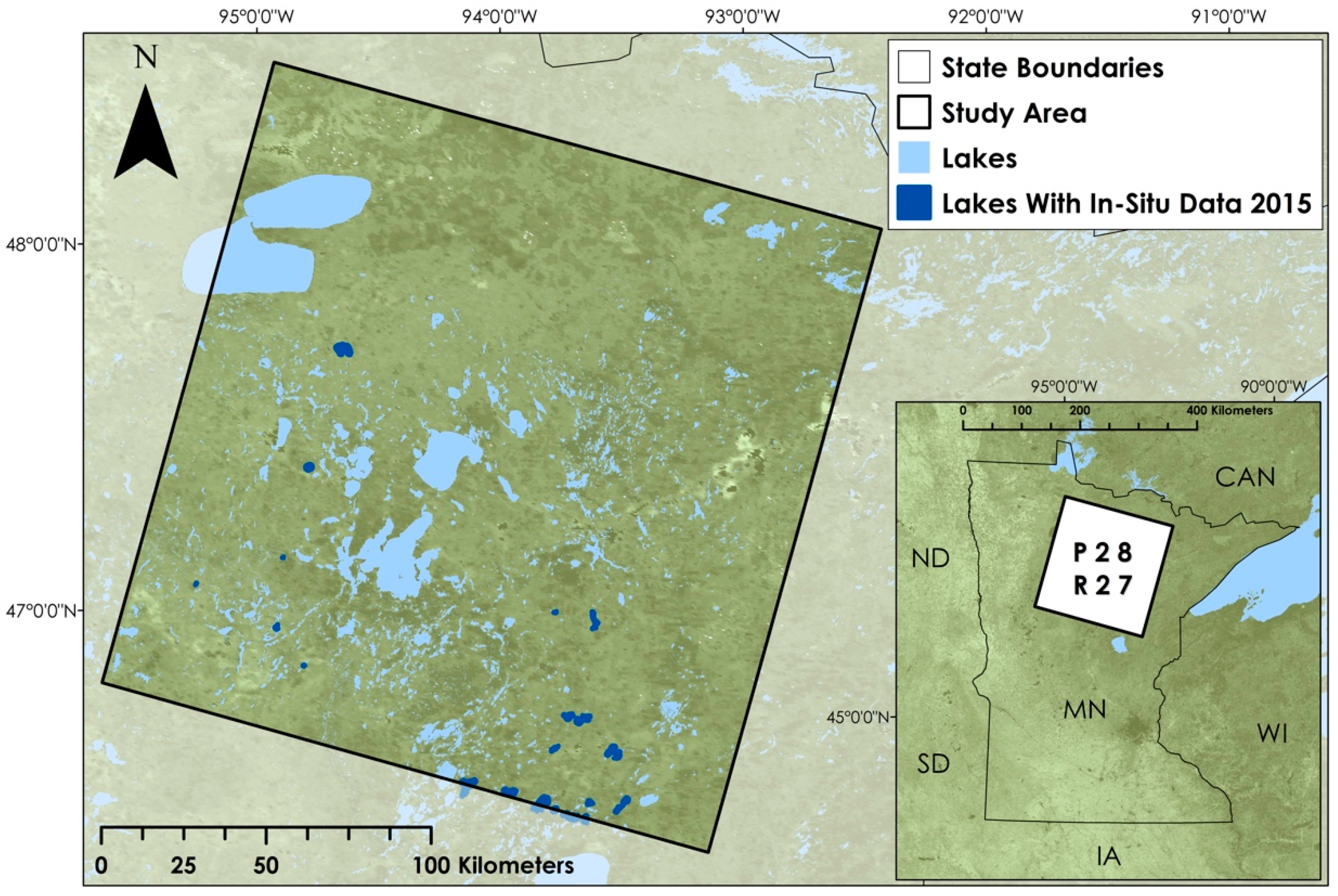
2.1. Study Area and Study Period

Our study area resides within the extent of a single Landsat scene (Worldwide Reference System 2, Path 28, Row 27) in north-central Minnesota (Figure 3) from June through September 2015. This area spans roughly 34,000 km2 and ranges from 330 to 560 m in elevation. The landscape is home to a vast network of rivers and lakes, and the unique wetland environments across the study area create ideal growing conditions for wildrice populations [3]. Cumulative precipitation in 2015 across the study area was 66.3 cm, which was approximately 1.3 cm greater than the 1895–2018 mean annual precipitation [22]. Field surveys were conducted across 30 lakes within the study region in 2015 (Figure 3) ranging from 0.1 to 11 km2 in size [23]. The lakes were mostly deep-water lakes, with diverse and extensive EAV in sheltered, shallow bays and narrow EAV fringes along shores of steep littoral slopes. Wildrice densities, which were not quantified, were highly variable across stands and lakes.

2.2. Training and Validation Datasets

The MN DNR monitors wildrice and all other EAV species through field surveys during mid to late summer by a team of botanists. During surveys, vegetation stands are mapped and digitized using Global Positioning System (GPS) and Geographic Information Systems (GIS) with spatial errors less than three meters of polygon boundaries [23]. To be included in these surveys, an EAV stand must cover more than 10 m2, and stands do not overlap [24]. Each EAV stand is classified into one of 11 classes, with the primary taxon being the dominant taxa in the stand, a secondary taxon could be listed (occurring in at least 30% of the stand), and associated taxa were recorded (occurring in less than 30% of the stand). These assessments are extremely valuable, but remain time-intensive, are not conducted annually or across all lakes, and exceptionally dense vegetation stands can prevent comprehensive data collection for many shallow lakes. Field survey polygon data, collected on deep lakes, were provided for this study by collaborators at the MN DNR. Training and validation data for all wildrice presence models were derived from the 2015 MN DNR survey polygons, which were concentrated in the southern half of our study area (Figure 3; Table 1). All species polygon presence data were reprojected into the WGS 1984 UTM 15N coordinate reference system, rasterized at 30 m spatial resolution, then aligned and clipped to the extent of Landsat Path 28, Row 27. The raster files were then converted to points and randomly subset to obtain separate training and validation datasets (Figure 2). These samples represent five different classes: wildrice, mixed wildrice and others, associated wildrice, wildrice absence, and open water (Table 1).
A total of 500 presence and 500 absence samples were generated for both training and validation of the base model. The training data generated from the surveys did include samples representing open water, so an additional 994 random absence samples were generated in areas both outside of the vegetation polygons and within the lakes. A Normalized Difference Vegetation Index (NDVI) threshold was then applied to ensure these locations represented water rather than unmapped vegetation. To determine an appropriate NDVI threshold, open water points were ocularly sampled using National Agriculture Imagery Program (NAIP) 1 m imagery [25] and NDVI values from Landsat 8 data were extracted at each of the points. Samples with NDVI greater than a threshold of −0.25 were removed, leaving 847 open water samples. Finally, we randomly selected 200 open water samples for training and 199 open water for validation. The wildrice presence, other EAV (absence), and open water samples were used to train the base model.

2.3. Training and Validation Dataset Modifications

We hypothesized that treating the associated wildrice class as wildrice presence may confuse the base model since wildrice is not dominant at these locations and therefore, the wildrice spectral signal may not be detected at a 30 m resolution. In the second model tested, the dominant taxa model, training data presences were removed where wildrice was not the dominant species (Figure 2). Presence training data were filtered to only include the wildrice and wildrice and others classes and EAV absences were randomly selected to balance between classes (Table 1). The base model validation dataset was parsed down using the same constraints to exclude associated wildrice from the presence samples.
For our third model, the threshold model, we further refined the presence samples utilized in the dominant taxa model by thresholding the samples based on their SAR signature (Figure 2 and Figure 4) to remove any presence samples that may not represent wildrice or contain a low proportion of nondominant wildrice cover (Table 1). First, we excluded the associated wildrice class from the training dataset utilizing the same methods we employed in the dominant taxa model. We then applied a SAR threshold to the training data to exclude samples potentially representing other nondominant species occurring within the wildrice and mixed wildrice presence polygons. Through preliminary testing, the range of the VV polarization between T1 and T2 consistently provided the greatest explanatory power for identifying wildrice in models; therefore, we utilized it to identify a threshold value to isolate samples dominated by wildrice. The mean, median, minimum, and maximum VV range values were used alongside distribution plots to characterize the observed values of wildrice presence, other EAV (absence), and open water. The median VV range value of other EAV was –0.5 and was selected as the threshold value to refine the wildrice presences (Figure 4). For the validation dataset, wildrice presences were filtered to exclude the associated wildrice class (Table 1), and 257 samples with VV range values less than −0.5 were selected for validation.

2.4. Satellite-Derived Spectral Data

All 2015 satellite imagery and datasets were acquired and processed using Google Earth Engine (GEE; [26]; Appendix A Table A1). The distinctive phenological traits of wildrice guided imagery selection. We used Landsat 8 Operational Land Imager (OLI) Tier 1 top-of-atmosphere reflectance images (30 m) [27,28] from the floating leaf/emergence stage (T1: June through July) and peak growth and harvest stage (T2: August through September). We applied a cloud filter to obtain images with a ≤35% cloud cover. An image composite for each time step was produced by taking the median value of each pixel. Reflectance bands, vegetation and moisture indices, and Tasseled Cap components (wetness, brightness, and greenness) [29] were derived from these median image composites to use as predictor variables. Sentinel-1 extrawide swath C-band SAR 10 m was processed and resampled to a 30 m resolution [30]. Median composite SAR bands for T1 and T2 were used to calculate ratios, range, and variance for both the VV and VH polarizations (Appendix A Table A1).

2.5. Modeling

We generated the base, dominant taxa, and threshold models using the random forest algorithm. Random forest is a machine learning technique that generates large numbers of decision trees using random subsets of training data and predictor variables [31]. First, the values of predictor variables (Appendix A Table A1) at each training and validation sample location were extracted in GEE and exported for variable selection and modeling using the R statistical software (Figure 2) [32]. Prior to generating each of the models, we utilized the Variable Selection Using Random Forests R package (VSURF, version 1.0.3 for selecting predictor variable combinations with the greatest explanatory power [33]. Using the outputs from VSURF, we tested the Pearson’s correlation of the top variables; for each pair of highly correlated variables (|r| > 0.75), the variable with the least explanatory power was removed. Random forest models were run [34], combining species presence and absence data with satellite-derived environmental variables to produce three binary classifications of wildrice presence and absence.

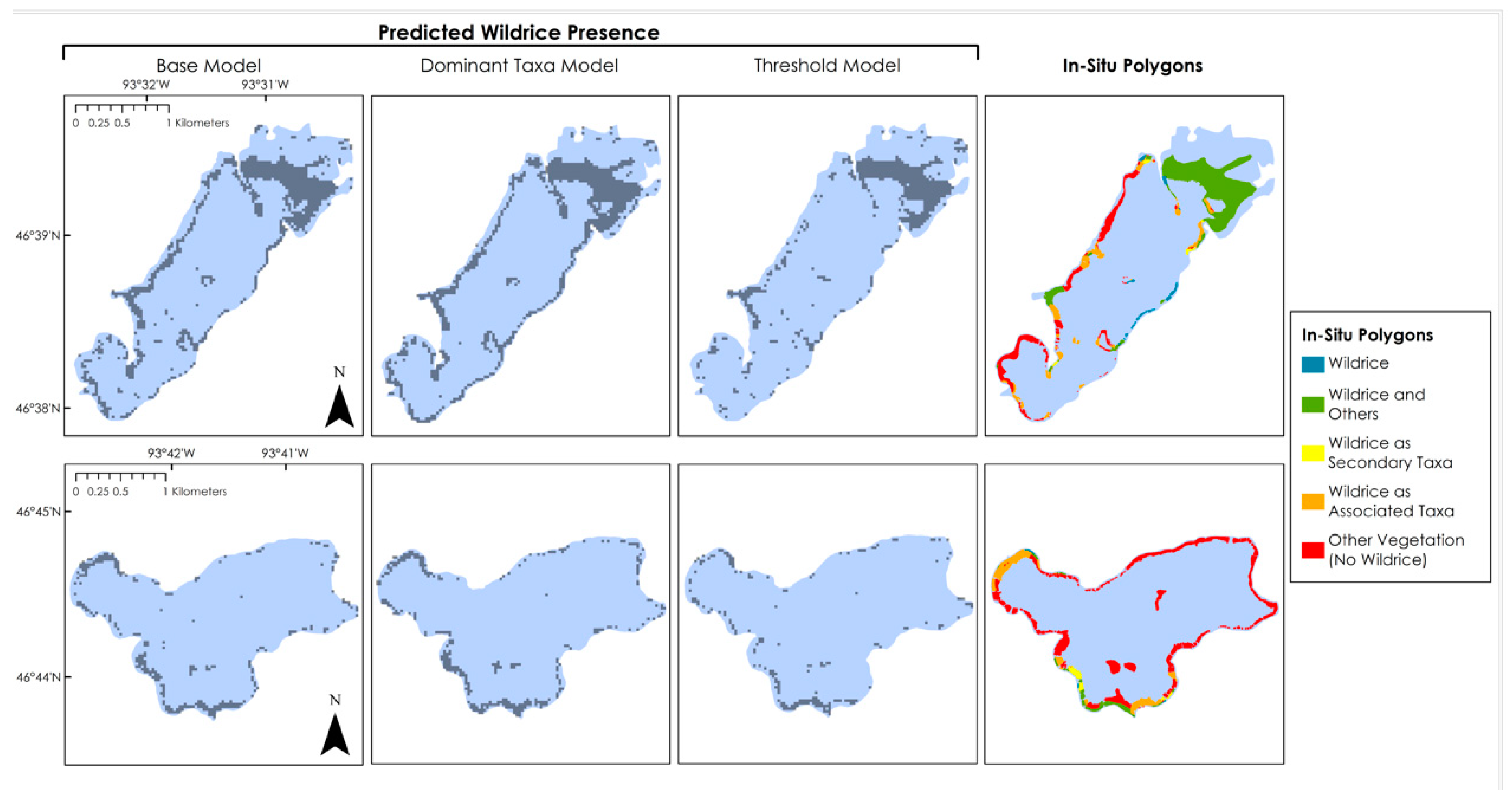
2.6. Point vs. Area-Based Validation

Two methods were used to assess the agreement between the survey polygons and each of the model’s predictive outputs: point accuracy and survey polygon “area of overlap” (Figure 2). The validation samples created from the MN DNR survey data were used to evaluate all three detection models. Models were applied to the presence and absence validation samples to determine classification accuracies using confusion matrices, sensitivity, and specificity [35] using the ‘caret’ R package [36]. Misclassified vegetation was further examined to determine which EAV classes were most frequently confused with wildrice. The models were not only validated with their corresponding validation set, but also with the validation set(s) of the subsequent models (Appendix A Table A2).
Model predictions were also overlaid on the 2015 MN DNR survey polygons to estimate the percentage of the total survey area correctly and incorrectly classified. Polygons were modified to match the resolution of the spatial imagery for direct comparisons using the following techniques. First, the survey polygons were converted to 1 m rasters and aligned with the model prediction rasters. Using the Aggregate tool in ArcMap (10.4.1), the 1 m rasters were resampled to 30 m. The sum of the resulting aggregate values represents the number of 1 m pixels (survey polygon area) within each 30 m pixel (resolution of the prediction rasters). Areas where the MN DNR survey polygons covered at least half of a pixel (aggregate values ≥ 450) were isolated and used for assessing the area of overlap between the model predictions and field data. The wildrice presence polygons also list secondary or additional taxa present, so a fraction of the area in each polygon contains the absence of wildrice (Table 1). Finally, all model predictions were overlaid to assess agreement between them; in particular, common trends can be summarized by two lakes (Gun and Esquagamah) that capture the spectrum of model performance over lakes from high to low wildrice cover.

3. Results

3.1. Model Validation

The base model demonstrated strong capabilities to detect wildrice, and subsequent modifications revealed how training data inform predictions of wildrice with various tradeoffs (Appendix A Table A2). Despite having lower wildrice class accuracy than the threshold model (Table 2), the base and dominant taxa models yielded similar and higher overlap with survey polygons (Figure 5). The dominant taxa model had higher overall accuracy, higher specificity, and in contrast to our expectations, lower sensitivity than the base model (Table 2). Despite having lower sensitivity, its predictions yielded higher overlap with wildrice presence polygons (Figure 5). The dominant taxa model predicted the largest area of wildrice presence and provided the most inclusive range, while also having the highest false positive overlap rate out of the models (Figure 5). An example of a high rate of false positives can be seen along the shoreline of Gun Lake with a greater frequency than the base model (Figure 6). The threshold model had the highest sensitivity and specificity (Table 2), yet the predictions from this model yielded the lowest overlap with survey polygons (Figure 5). This model did not capture the full range of wildrice presence, but it had the lowest false positive error rates in both the point and percent overlap validation. It is visually apparent that the threshold model has the lowest true and false positive error rates across Gun Lake and Esquagamah Lake (Figure 6). While the threshold model detected the smallest area of wildrice presence, the predictions from this model had the highest true positive/negative percentage.
Larger patches of wildrice presence were associated with a high rate of agreement between all three models (Figure 7). The largest model agreement patch on the northeast end of Gun Lake (Figure 7) is consistent with the largest survey polygon (Figure 6) representing wildrice presence (wildrice and others) on this lake. The least agreement between all models coincides with wildrice presence polygons that have dimensions smaller than a Landsat pixel, as shown across the eastern shore of Gun Lake (Figure 7). It is visually apparent that all models struggle to detect wildrice at a subpixel spatial resolution. The base and threshold models had similar sporadic false positive errors across open water, which aligned in many spots on the southern half of Gun Lake (Figure 7). The dominant taxa model did not have the same false positive errors on open water, which is likely a result of the greater number of different predictors it utilized.
Percent correctly classified for all three models consistently increased when cross-validated using corresponding and noncorresponding datasets to determine point accuracy (Appendix A Table A2). This provided insight on how the modifications performed across each validation set and demonstrated that low density or sparse wildrice presence points included in training data for the base and dominant taxa models were responsible for inflated false positive errors in their validation accuracies and polygon validation (Figure 5). The base model followed a trend of increasing wildrice class accuracy when applied to the subsequently modified validation sets with a trade-off of decreased absence class accuracy (Appendix A Table A2). The dominant taxa model also increased in wildrice class accuracy and decreased in absence accuracy when applied to the threshold model’s validation set. Applying dominant taxa and threshold models to validation datasets without corresponding modifications followed a consistent trend of decreasing accuracy because previous validation sets still contained more low density or sparse wildrice presence points. Applying models backward through the process inflated false negative errors.

3.2. Predictor Variable Performance

The VV range consistently contributed the greatest explanatory power to wildrice detection across all models which aligns with results from Gallant et al. [17]. The other predictors performed similarly across models and ranking order was the primary difference between them (Figure 8). The majority of SAR derived predictor variables were ranked as top predictors by VSURF. However, many SAR variables were highly correlated with the VV range but did not outperform the VV range in any of the models. The blue and ultrablue spectral band values from the second time period of interest also played a role in the detection of wildrice (Figure 8). In general, the second time period (August–September) had the greatest number of variables that correlated with wildrice presence. In the context of the annual life cycle of wildrice, it makes ecological sense for the second time period to contain the most important variables, because it corresponds with peak annual growth.
Throughout all of the point accuracy assessments, bulrushes contributed to the greatest number of false positive errors followed by water lilies in approximate ratios of 3 bulrush false positives:1 water lilies false positive (base), 2:1 (dominant), and 1:1 (threshold; Figure 9). The dominant taxa model contained an additional SAR predictor (VH range) that the base model did not (Figure 8; #5). In the threshold model, the importance of the VH range increased from the dominant taxa model (Figure 8). VH range adds information about horizontal scatter of EAV canopies [21] and is a factor contributing to the improvements in class accuracy of bulrushes (Figure 9).

4. Discussion

We describe a detailed and rigorously tested methodology that provides a significant step forward in mapping the extent of wildrice by incorporating a rich in-situ dataset, providing threshold values with associated justifications, and highlighting model performance compared to field surveys. Studies that previously mapped wildrice in Minnesota required manual and resource-intensive methods, and those utilizing remotely sensed data produced results that may be challenging to incorporate into local management decisions due to unclear accuracy. We utilized remote sensing datasets that are free, publicly available, and hosted through GEE, increasing the efficiency of mapping natural wildrice. Further, we validated our results using a robust field dataset which provided multiple measures of model evaluation not present in similar studies.
Our model accuracy was comparable to the classification results achieved by Brisco et al. [18] mapping rice (Oryza L.) paddies in Asia; however, we took additional steps to evaluate performance. We expected water lilies to be the EAV class most commonly confused with wildrice based on the frequent co-occurrence of the two [37], but this was not observed with the base or dominant taxa models (Figure 9; Appendix A Table A3). The base model had the highest misclassification rate of bulrushes, and the modifications applied to the dominant taxa model reduced this misclassification rate significantly by including additional information about horizontal canopy structure captured by the VH range [21]. However, bulrushes were still incorrectly classified as wildrice twice as often as water lilies with the dominant taxa model. Gallant et al. [17] found that VV thresholds improved separation between wildrice and bulrushes. The threshold model had the most SAR predictors that contributed greater explanatory power to the model (Figure 8) and this factor may have translated to the nearly even contributions between bulrushes and water lilies in the false positive error rate (Figure 9). This result was more similar to the expected occurrence patterns of these species and suggests that the VV range threshold applied refined the samples to more likely represent wildrice with density and cover great enough to be detected at a 30 m resolution.
We faced the challenge of modifying the rich information captured by survey polygons at a fine spatial resolution to compliment remotely sensed datasets with much coarser spatial resolution. Survey data available within our study area and time period imposed limitations on the training data. The difference in polygon area surveyed and the number of presence samples generated from each sample class (Table 1) is likely one factor that explains why all model predictions have the largest area of overlap with the mixed wildrice and others class (Figure 5). In many cases, field surveys are not collected for remote sensing purposes, and in this case, the surveys did not capture estimates of the cover, density, or the spatial distribution of each taxon within a polygon. We randomly generated samples within the survey polygons; based on field survey definitions and collection methods, a maximum of 30% of the area of wildrice polygons may represent other EAV which may alter the spectral signature captured by a single pixel from remotely sensed data at a 30 m resolution. The likelihood of randomly generated presence points being placed on other EAV taxa increases in the mixed wildrice and others class since other vegetation represents more than 30% of the total area in these polygons. Stands of EAV with multiple taxa, especially those that also contained a low cover of wildrice, provide a different spectral signature than those with higher cover or dominance of wildrice. Presence samples generated over areas with mixed or low densities of wildrice introduced confusion within all models, causing them to struggle with detecting low wildrice cover; this was most prevalent with the base model (Figure 9). Calculating overlap of model predictions across mixed classes of wildrice presence was the most challenging aspect of the polygon validation due to the natural heterogeneity of EAV stands and the variety of taxa present within each.
We found that multiple lines of validation were necessary to evaluate how well the models detected wildrice as documented by the field surveys. When considering point validation, we found the validation dataset to matter immensely. When applying models to more restrictive validation datasets, sensitivity increases because additional restrictions reduced the number of low density or mixed wildrice points. Inversely, applying models to more inclusive validation datasets results in a trend of decreasing sensitivity because models are challenged with correctly classifying more mixed or sparse wildrice points (Appendix A Table A2). Additionally, the results of polygon validation did not linearly correspond to the point validations results, providing mixed indications about which model best-captured wildrice.
Each model demonstrated strong capabilities to detect wildrice, but the nuances between their performances elucidate the most appropriate applications of each. The full extent of wildrice occurrence predicted by each model cannot be used to estimate biomass, stand density, or be assumed to be representative of additional years beyond 2015 due to the interannual variability of wildrice stand densities. The dominant taxa model predicted the most wildrice area and had the greatest area of overlap with surveyed wildrice polygons. Since it performed most accurately via visual inspection with larger stands of wildrice and EAV (equivalent to the size of multiple adjacent Landsat pixels), it is more likely to be accurate where there are patches of predicted presence. Since it has the highest false positive error rate, individual presence pixels or very small patches of presence pixels are less likely to be accurate. The dominant taxa model balanced false positive errors across species (Figure 9) while maintaining more inclusive predictions than the base model (Figure 5). Therefore, the dominant taxa model may be better suited for estimating the full range of wildrice occurrence, including where wildrice is an associated and secondary species present. The base model could be applied similarly to the dominant taxa model. In contrast to these models, the threshold model may be more relevant at a local scale to guide field surveys to monitor wildrice during its short annual growing season. While it did not detect as much wildrice as the other models, it has higher true positive and lower false positive error rates in both validation processes. This is most notable through the polygon validation where the threshold model had half the rate of overlap with the absence of polygons when compared to the dominant taxa model (Figure 5). The methods used to generate the threshold model could be applied to current imagery, and the resulting maps may be useful to maximize the time and resource efficiency of collecting field data at unsurveyed locations. In future surveys, including estimates of cover and taxa distribution within a polygon could improve model accuracy within mixed stands of EAV and allow for more rigorous validation. Another approach could include isolating more homogenous EAV stands in separate polygons and making note of respective densities.

5. Conclusions

Our study demonstrated that combining remotely sensed data and detailed field surveys into models can provide comprehensive predictions of wildrice extent with clear accuracy metrics and repeatable methodology that can be applied to map wildrice across broader regions of interest. These promising results indicate a high potential to support food security and conservation efforts by increasing the information available to land management and reducing the time and resources required to survey wildrice across its native range. This is a stepping stone to performing long-term monitoring of wildrice abundance on lakes where wildrice is especially important from ecological and cultural perspectives. Future research should consider testing the applicability of these models across multiple years to assess temporal accuracy as well as the feasibility of applying similar methods for mapping other crops’ wild relative species to monitor natural crop persistence amidst changes in climate. Annual maps are necessary to evaluate the trends and dynamics of wildrice stands and would extend to quantifying the decline in native wildrice stands. Additional testing and refinement of the outlined methods would support quantification of the impacts that systemic drivers have on wildrice populations, improve broadscale efforts to effectively conserve wildrice, and ultimately promote long-term food security.

Author Contributions

Conceptualization, T.M., P.R., C.K.K., A.K., and P.E.; methodology, A.V., N.Y., J.L., K.O., D.C., V.M., T.M., and E.S.; software, J.L., D.C., K.O., E.S. and V.M.; validation, J.L., A.V., N.Y., A.K.K., and K.O.; formal analysis, J.L., E.S., K.O., A.V., D.C., V.M., T.M., and N.Y.; investigation, J.L., D.C., E.S., K.O., and V.M.; resources, P.R., J.K., P.E., C.K.K., and A.K.; data curation, J.L., K.O., J.K., E.S., V.M., T.M., and D.C.; writing—original draft preparation, K.O., J.L., A.V., E.S., N.Y., and V.M.; writing—review and editing, All Authors; visualization, J.L., K.O.; supervision, T.M., A.V., P.E., C.K.K., and N.Y.; project administration, T.M., A.V., P.E., C.K., and N.Y.; funding acquisition, C.K., P.E. All authors have read and agreed to the published version of the manuscript.

Funding

This research was funded by USDA Agricultural Research Service (award #007271-00002). The USDA is an equal opportunity employer and provider. Support was also provided by the National Aeronautics and Space Administration through contract NNL16AA05C and cooperative agreement NNX14AB60A. Any opinions, findings, and conclusions or recommendations expressed in this material are those of the authors and do not necessarily reflect the views of the National Aeronautics and Space Administration.

Acknowledgments

We would like to thank Katie Walker, Charles Whittemore, and Leorah McGinnis from the NASA DEVELOP program for their support of preliminary method development. We also thank Ann Geisman, Stephanie Simon, Donna Perleberg, and Calub Shavlik from the Minnesota Department of Natural Resources for providing data, local insight, and expert knowledge of the area.

Conflicts of Interest

The authors declare no conflict of interest.

Data Availability

The MN DNR data is available through the MN Data Practices Act at https://mn.gov/admin/data-practices/data/.

Appendix A

Table A1. Spectral/radar derivatives utilized in satellite detection modeling of wildrice.
Spectral DerivativeEquationDescriptionSource
Normalized Difference Vegetation Index (NDVI)NDVI = (NIR − Red)/(NIR + Red)A remote sensing indicator that can be used to assess vegetation content[38]
Normalized Difference Moisture Index (NDMI)NDMI = (NIR − SWIR)/(NIR + SWIR)A remote sensing indicator that can be used to assess water content[38]
Tasseled Cap WetnessBlue (0.1511) + Green (0.1973) + Red (0.3283) + NIR (0.3407) + SWIR (−0.7117) + SWIR2 (−0.4559)A linear transformation of spectral bands, used to distinguish wet surfaces and measure water content[39]
Tasseled Cap GreennessBlue (−0.2941) + Green (−0.243) + Red (−0.5424) + NIR (0.7276) + SWIR (0.0713) + SWIR2 (−0.1608)A linear transformation of spectral bands, used to distinguish vegetated surfaces and measure vegetation content[28]
Tasseled Cap BrightnessBlue (0.3029) + Green (0.2786) + Red (0.4733) + NIR (0.5599) + SWIR (0.508) + SWIR2 (0.1872)A linear transformation of spectral bands, used to distinguish bright surfaces and measure brightness content[28]
Radar RangeRadar Median T1 − Radar Median T2The range of the radar backscatter signal over the growing season (T1: June–July, T2: August–September)[17]
Radar Variance s 2 = ( x X ¯ ) 2 N 1 The variance of the radar backscatter signal over the growing season
Radar Cross-Ratio(Radar VV Median)/Radar (VH) Median or (Radar VH Median)/Radar (VV) MedianThe ratio of VV and VH radar polarizations for a certain time period.
Table A2. Model evaluation metrics comparing overall and class accuracy between all models, with associated confusion matrices.
ModelValidation SetPCCSensitivity
(Presence Accuracy)
Specificity
(Absence Accuracy)
Confusion Matrix
TPTNFPFN
BaseBase83.8%83.3%84.2%3655239873
83.3%84.2%15.8%16.7%
BaseDominant Taxa83.5%86.0%82.1%2574379542
86.0%82.1%17.9%14.0%
Base Threshold85.0%91.1%82.1%2344379523
91.1%82.1%17.9%14.0%
Dominant TaxaDominant Taxa87.5%81.6%90.8%2444834955
81.6%90.8%9.2%18.4%
Dominant TaxaBase79.6%64.7%90.2%28256061154
64.7%90.2%9.8%35.3%
Dominant TaxaThreshold 90.0%87.9%91.0%2264844831
87.9%91.1%9.0%12.1%
Threshold Threshold91.1%89.5%92.0%2304594027
89.5%92.0%8.0%10.5%
ThresholdDominant Taxa85.6%76.3%90.8%2284834971
76.3%90.8%9.2%23.7%
ThresholdBase79.4%62.2%91.5%27156853165
62.2%91.5%8.5%37.8%
Table A3. False positive breakdown for each model validated on each validation set.
Model TrainedModel ValidatedTotal False PositivesRushesWater LiliesRushes and OthersWater lilies and OthersOtherTotal Vegetation Absence Points
BaseBase984515131015422
BaseDominant Taxa954114101119333
BaseThreshold954114101119300
Dominant TaxaBase61231310510422
Dominant TaxaDominant Taxa492010757333
Dominant TaxaThreshold482010657300
ThresholdBase5321111029422
ThresholdDominant Taxa492211628333
ThresholdThreshold401210738300

References

  1. Pillsbury, R.W.; McGuire, M.A. Factors affecting the distribution of wild rice (Zizania palustris) and the associated macrophyte community. Wetlands 2009, 29, 724–734. [Google Scholar] [CrossRef]
  2. Drewes, A.D.; Silbernagel, J. Uncovering the spatial dynamics of wild rice lakes, harvesters and management across Great Lakes landscapes for shared regional conservation. Ecol. Model. 2012, 229, 97–107. [Google Scholar] [CrossRef]
  3. DNR. Natural Wild Rice in Minnesota; Minnesota Department of Natural Resources: St. Paul, MI, USA, 2008; p. 116. Available online: http://files.dnr.state.mn.us/fish_wildlife/wildlife/shallowlakes/natural-wild-rice-in-minnesota.pdf (accessed on 7 August 2019).
  4. Price, M.W. Spectral Identification of Wild Rice (Zizania Palustris L.) Using Indigenous Knowledge and Landsat Multispectral Data. Master’s Thesis, University of Montana, Missoula, MT, USA, 2012. [Google Scholar]
  5. Anderson, R.; Kapfer, P.; Ueland, J.; Lawrence, J.; Cordts, S. Comparison of Wild Rice and Waterfowl Surveys. 2011. Available online: https://www.lccmr.leg.mn/projects/2011/finals/2011_04j_2e_rpt_wild-rice-data-waterfowl-surveys.pdf (accessed on 29 June 2020).
  6. Kennard, W.; Porter, R.; Grombacher, A.; Phillips, R.L. A comparative map of wild rice (Zizania palustris L. 2n = 2x = 30). Theor. Appl. Genet. 1999, 99, 793–799. [Google Scholar] [CrossRef]
  7. Khoury, C.K.; Greene, S.; Wiersema, J.H.; Maxted, N.; Jarvis, A.; Struik, P.C. An inventory of crop wild relatives of the United States. Crop Sci. 2013, 53, 1496–1508. [Google Scholar] [CrossRef]
  8. Biesboer, D.D. The ecology and conservation of wild rice, Zizania palustris L., in North America. Acta Limnol. Bras. 2019, 31. [Google Scholar] [CrossRef] [Green Version]
  9. Rickman, D.L.; Greensky, W.A.; Al-Hamdan, M.Z.; Estes, M.G.; Crosson, W.L.; Estes, S.M. Spatial and Temporal Analyses of Environmental Effects on Zizania palustris and Its Natural Cycles. NASA Technical Reports Server. 2017. Available online: https://ntrs.nasa.gov/search.jsp?R=20170010653 (accessed on 29 June 2020).
  10. Oelke, A.E.; Teynor, T.M.; Carter, P.R.; Percich, J.A.; Noetzel, D.M.; Bloom, P.R.; Porter, A.R.; Schertz, C.E. Wild rice. In Alternative Field Crops Manual; University of Minnesota: St. Paul, MN, USA, 1997; pp. 315–334. [Google Scholar]
  11. Rundquist, D.C.; Narumalani, S.; Narayanan, R.M. A review of wetlands remote sensing and defining new considerations. Remote. Sens. Rev. 2001, 20, 207–226. [Google Scholar] [CrossRef]
  12. Gonoski, J.; Burk, T.E.; Bolstad, P.V.; Balogh, M. Rice Lake National Wildlife Refuge Historic Wild Rice Mapping (1983–2004); College of Natural Resources and Minnesota Agricultural Experiment Station, University of Minnesota: St. Paul, MN, USA, 2005. [Google Scholar]
  13. Kontgis, C.; Schneider, A.; Ozdogan, M. Mapping rice paddy extent and intensification in the Vietnamese Mekong River Delta with dense time stacks of Landsat data. Remote Sens. Environ. 2015, 169, 255–269. [Google Scholar] [CrossRef]
  14. Dong, J.; Xiao, X.; Menarguez, M.A.; Zhang, G.; Qin, Y.; Thau, D.; Biradar, C.; Moore, B. Mapping paddy rice planting area in northeastern Asia with Landsat 8 images, phenology-based algorithm and Google Earth Engine. Remote Sens. Environ. 2016, 185, 142–154. [Google Scholar] [CrossRef] [Green Version]
  15. Torbick, N.; Chowdhury, D.; Salas, W.; Qi, J. Monitoring rice agriculture across Myanmar using time series Sentinel-1 assisted by Landsat-8 and PALSAR-2. Remote Sens. 2017, 9, 119. [Google Scholar] [CrossRef] [Green Version]
  16. Mansaray, L.R.; Huang, W.; Zhang, D.; Huang, J.; Li, J. Mapping rice fields in urban Shanghai, Southeast China, using Sentinel-1A and Landsat 8 datasets. Remote Sens. 2017, 9, 257. [Google Scholar] [CrossRef] [Green Version]
  17. Gallant, A.L.; Kaya, S.G.; White, L.; Brisco, B.; Roth, M.F.; Sadinski, W.; Rover, J. Detecting emergence, growth, and senescence of wetland vegetation with polarimetric Synthetic Aperture Radar (SAR) data. Water 2014, 6, 694–722. [Google Scholar] [CrossRef] [Green Version]
  18. Brisco, B.; Li, K.; Tedford, B.; Charbonneau, F.; Yun, S.; Murnaghan, K. Compact polarimetry assessment for rice and wetland mapping. Int. J. Remote Sens. 2012, 34, 1949–1964. [Google Scholar] [CrossRef] [Green Version]
  19. Chen, C.F.; Son, N.T.; Chen, C.R.; Chang, L.Y.; Chiang, S.H. Rice crop mapping using Sentinel-1A phenological metrics. Int. Arch. Photogramm. Remote Sens. Spat. Inf. Sci. 2016, 41, 863–865. [Google Scholar]
  20. Lasko, K.; Vadrevu, K.P.; Tran, V.T.; Justice, C. Mapping double and single crop paddy rice with Sentinel-1A at varying spatial scales and polarizations in Hanoi, Vietnam. IEEE J. Sel. Top. Appl. Earth Obs. Remote Sens. 2018, 11, 498–512. [Google Scholar] [CrossRef] [PubMed]
  21. Silva, T.; Costa, M.P.F.; Melack, J.M.; Novo, E.M.L.M. Remote sensing of aquatic vegetation: Theory and applications. Environ. Monit. Assess. 2007, 140, 131–145. [Google Scholar] [CrossRef]
  22. MNDR. (n.d). Minnesota Climate Trends 1895–2018. Available online: https://arcgis.dnr.state.mn.us/ewr/climatetrends/) (accessed on 29 June 2020).
  23. Radomski, P.; Woizeschke, K.; Carlson, K.; Perleberg, D. Reproducibility of emergent plant mapping on lakes. N. Am. J. Fish. Manag. 2011, 31, 144–150. [Google Scholar] [CrossRef]
  24. Perleberg, D.; Radomski, P.; Simon, S.; Carlson, K.; Knopik, J. Minnesota Lake Plant Survey Manual, for Use by MNDNR Fisheries Section and EWR Lake Habitat Program; Minnesota Department of Natural Resources, Ecological and Water Resources Division: Brainerd, MN, USA, 2016; 128p. [Google Scholar]
  25. United States Department of Agriculture (USDA). Farm Service Agency. National Agriculture Imagery Program (NAIP) [Image collection]. Google Earth Engine API. 2015. Available online: https://code.earthengine.google.com/ (accessed on 20 February 2019).
  26. Gorelick, N.; Hancher, M.; Dixon, M.; Ilyushchenko, S.; Thau, D.; Moore, R. Google Earth Engine: Planetary-scale geospatial analysis for everyone. Remote Sens. Environ. 2017, 202, 18–27. [Google Scholar] [CrossRef]
  27. United States Geological Survey (USGS). Earth Resources Observation and Science Center. Landsat 8 OLI Level-2 Surface Reflectance (SR) Science Product. 2014. Available online: https://www.usgs.gov/centers/eros/science/usgs-eros-archive-landsat-archives-landsat-8-olitirs-level-2-data-products?qt-science_center_objects=0#qt-science_center_objects (accessed on 20 February 2019).
  28. Young, N.E.; Anderson, R.; Chignell, S.M.; Vorster, A.G.; Lawrence, R.; Evangelista, P.H. A survival guide to Landsat preprocessing. Ecology 2017, 98, 920–932. [Google Scholar] [CrossRef] [Green Version]
  29. Baig, M.H.A.; Zhang, L.; Shuai, T.; Tong, Q. Derivation of a tasselled cap transformation based on Landsat 8 at-satellite reflectance. Remote Sens. Lett. 2014, 5, 423–431. [Google Scholar] [CrossRef]
  30. Copernicus Sentinel Data (2015). Retrieved from Google Earth Engine [4 February 2019], processed by ESA.
  31. Breiman, L.; Last, M.; Rice, J. Random Forests. Mach. Learn. 2001, 45, 5–32. [Google Scholar]
  32. R Core Team. R: A Language and Environment for Statistical Computing; R Foundation for Statistical Computing: Vienna, Austria, 2013. [Google Scholar]
  33. Genuer, R.; Poggi, J.-M.; Tuleau-Malot, C. VSURF: An R package for variable selection using random forests. R J. 2015, 7, 19–33. [Google Scholar] [CrossRef] [Green Version]
  34. Liaw, A.; Wiener, M. Classification and regression by randomforest. R News 2002, 2, 18–22. [Google Scholar]
  35. Shabani, F.; Kumar, L.; Ahmadi, M. Assessing accuracy methods of species distribution models: AUC, specificity, sensitivity and the true skill statistic. Glob. J. Hum. Soc. Sci. B 2018, 18, 7–18. [Google Scholar]
  36. Kuhn, M. Caret package. J. Stat. Softw. 2008, 28. [Google Scholar]
  37. Myrbo, A.; Swain, E.B.; Engstrom, D.R.; Wasik, J.C.; Brenner, J.; Shore, M.D.; Peters, E.B.; Blaha, G. Sulfide generated by sulfate reduction is a primary controller of the occurrence of wild rice (Zizania palustris) in shallow aquatic ecosystems. J. Geophys. Res. Biogeosci. 2017, 122, 2736–2753. [Google Scholar] [CrossRef] [Green Version]
  38. Xiao, X.; Boles, S.; Liu, J.; Zhuang, D.; Frolking, S.; Li, C.; Salas, W.; Moore, B. Mapping paddy rice agriculture in southern China using multi-temporal MODIS images. Remote Sens. Environ. 2005, 95, 480–492. [Google Scholar] [CrossRef]
  39. Jin, S.; Sader, S.A. Comparison of time series tasseled cap wetness and the normalized difference moisture index in detecting forest disturbances. Remote Sens. Environ. 2005, 94, 364–372. [Google Scholar] [CrossRef]
Figure 1. The annual life cycle of northern wildrice.
Remotesensing 12 03023 g001
Figure 2. Flowchart that illustrates and describes the refinement of training and validation data that characterizes each of the three wildrice models (Base Model, Dominate Taxa Model, and Threshold Model), the modeling process to map wildrice, and the model validation.
Remotesensing 12 03023 g002
Figure 3. Study area extent in north-central Minnesota, USA (Landsat Path 28, Row 27).
Remotesensing 12 03023 g003
Figure 4. The frequency and distribution of Vertical Vertical (VV) range values for 333 wildrice presence, 333 other emergent aquatic vegetation (absence), and 200 open water samples were used to determine the optimal threshold for presence samples. A threshold of −0.5 was selected, which corresponds with the median value of absence points, to eliminate other taxa present in mixed stands of wildrice and isolate the signature of wildrice.
Remotesensing 12 03023 g004
Figure 5. Percent overlap between model predictions and in-situ polygons covering at least half the area of a pixel (30 m). Reference in-situ survey cover definitions in Table 1 to clarify the species included in each class with respect to their proportion of cover and dominance. Note that wildrice does not comprise the full area surveyed for any of the classes and therefore will not constitute 100% of the total area for any of the model predictions. Results based on validation over 30 lakes.
Remotesensing 12 03023 g005
Figure 6. Comparison of predicted wildrice presence between all three models across Gun Lake (top row) and Esquagamah Lake (bottom row). Gun Lake is representative of trends observed across lakes with high cover of wildrice while Esquagamah Lake highlights trends across lakes with low wildrice cover; these examples cover the spectrum of predictive patterns. Each set of model predictions shown in gray (columns one through three) were compared to the in-situ data collected across the two lakes which represent the extent of wildrice presence and absence surveyed in 2015 (column four).
Remotesensing 12 03023 g006
Figure 7. Agreement between model predictions of wildrice presence in 2015 across Gun Lake (left) and Esquagamah Lake (right).
Remotesensing 12 03023 g007
Figure 8. Top model predictor variables ranked by relative variable importance derived from the mean decrease in accuracy.
Remotesensing 12 03023 g008
Figure 9. The number of absence samples misclassified as wildrice from each taxon for each model modification when applied to its corresponding validation set (i.e., base model applied on base validation dataset, etc.). General proportions of misclassification are preserved when validated on noncorresponding validation sets (i.e., base model applied to threshold validation dataset, etc.) (Appendix A Table A2). Vegetation absence points included for the base, dominant taxa, and threshold models were 422, 333, and 300 respectively.
Remotesensing 12 03023 g009
Table 1. Training and Validation Data Descriptions: Shows point classes, the taxa included in each class, and the number of sample points used to train each model.
Sample ClassPrimary TaxaSecondary TaxaAssociated Taxa Number of Training Data Points
Dominant Vegetation<Dominant Cover and >30% Cover<30% CoverBase ModelDominant Taxa ModelThreshold Model
Wildrice 111111
Mixed Wildrice and Others322322283
Associated Wildrice•◦•◦16700
Wildrice Absence500333300
Open Water 200200199
• represents wildrice presence, ◦ represents other aquatic vegetation presence, no denotation represents the absence of wildrice and aquatic vegetation. The wildrice class represents areas where wildrice is the dominant species in a mostly monotypic stand and any additional emergent aquatic vegetation (EAV) taxa present makes up <30% of the total stand [24]. The mixed wildrice and others class is where wildrice is the dominant species in a mixed stand and at least one other species represents secondary species making up 30% or more of the stand of EAV. The associated wildrice class has wildrice listed as secondary or other taxa present taking up 30% (secondary taxa > 30%) or less (other taxa < 30%) of the total area, but it is not the dominant species. For the absence of wildrice class, wildrice is not listed as a primary, secondary, or associated taxa present within a stand of EAV. The open water class is absent from all aquatic vegetation.
Table 2. Point validation metrics comparing percent correctly classified (PCC), sensitivity, and specificity between all models, with associated confusion matrices. Cross-validation between models and associated metrics located in Appendix A Table A2.
ModelValidation SetPCCSensitivity
(Presence Accuracy)
Specificity
(Absence Accuracy)
Confusion Matrices
TPTNFPFN
BaseBase83.8%83.3%84.2%3635239873
83.3%84.2%15.8%16.7%
Dominant TaxaDominant Taxa87.5%81.6%90.8%2444834955
81.6%90.8%9.2%18.4%
Threshold Threshold91.1%89.5%92.0%2304594027
89.5%92.0%8.0%10.5%

