Comparison of Filters for Archaeology-Specific Ground Extraction from Airborne LiDAR Point Clouds


1
Research Centre of the Slovenian Academy of Sciences and Arts, Novi trg 2, 1000 Ljubljana, Slovenia
2
Institute of Classics, University of Graz, Universitätsplatz 3/II, 8010 Graz, Austria
*
Author to whom correspondence should be addressed.
Remote Sens. 2020, 12(18), 3025; https://0-doi-org.brum.beds.ac.uk/10.3390/rs12183025
Submission received: 20 July 2020
/
Revised: 11 September 2020
/
Accepted: 15 September 2020
/
Published: 16 September 2020
Abstract
:Identifying bare-earth or ground returns within point cloud data is a crucially important process for archaeologists who use airborne LiDAR data, yet there has thus far been very little comparative assessment of the available archaeology-specific methods and their usefulness for archaeological applications. This article aims to provide an archaeology-specific comparison of filters for ground extraction from airborne LiDAR point clouds. The qualitative and quantitative comparison of the data from four archaeological sites from Austria, Slovenia, and Spain should also be relevant to other disciplines that use visualized airborne LiDAR data. We have compared nine filters implemented in free or low-cost off-the-shelf software, six of which are evaluated in this way for the first time. The results of the qualitative and quantitative comparison are not directly analogous, and no filter is outstanding compared to the others. However, the results are directly transferable to real-world problem-solving: Which filter works best for a given combination of data density, landscape type, and type of archaeological features? In general, progressive TIN (software: lasground_new) and a hybrid (software: Global Mapper) commercial filter are consistently among the best, followed by an open source slope-based one (software: Whitebox GAT). The ability of the free multiscale curvature classification filter (software: MCC-LIDAR) to remove vegetation is also commendable. Notably, our findings show that filters based on an older generation of algorithms consistently outperform newer filtering techniques. This is a reminder of the indirect path from publishing an algorithm to filter implementation in software.
1. Introduction
Airborne light detection and ranging (LiDAR) is now widely used in archaeological prospection [1,2]. Archaeologists interpret enhanced visualizations of airborne LiDAR-derived high-resolution digital terrain models (DTMs) with a combination of perception and comprehension, e.g., [3,4]. The results have proven to be very successful in detecting archaeological features and have uncovered numerable new settlements and almost innumerable new archaeological features worldwide, e.g., recently [5,6,7,8,9].
Airborne LiDAR-derived data provide archaeologists with detailed topography, which is a powerful resource for interpretation [10]. The often described process from data acquisition to archaeological interpretation [11,12,13,14,15,16] can be divided for the purposes of this article into raw data processing (project planning, system calibration, data acquisition, georeferencing, flight strip adjustment), point cloud processing (ground point filtering, additional processing), creation of end products (archaeology-specific raster elevation model interpolation and it visualization), and archaeological interpretation (interpretative mapping, ground inspection, deep integrated multi-scale interpretation). For archaeology, the most critical part of the workflow is ground point filtering [16], and this is the subject of our article.
It is worth reiterating that this process involves assumptions and decisions during the entire workflow, but these are often underestimated or even ignored [12,13]. As some of the end products (for example, a simple hill-shaded representation of the DTM) are almost self-explanatory, this may lead to a certain ignorance of the underlying data processing strategies [16].
In comparison to other fields the use of airborne LiDAR-derived data in archaeology is specific in several ways. First, visual inspection of enhanced raster visualizations remains the key method. The digital surface model (DSM) used often combines a digital terrain model (DTM) with off-terrain archaeological features [16] and modern buildings [10,17,18]. Such a specific DSM has been termed the digital feature model (DFM) [19].
Secondly, morphologically speaking archaeological features are anomalies, i.e., sporadically occurring atypical features of the terrain. The direct application of existing generic methods developed to assess the average accuracy of the terrain [20] is, therefore, less than ideal. For example, in archaeology, low noise can be tolerated as long as the size of the distortion is significantly smaller than the archaeological features.
Third, the time, effort, equipment, and human resources invested in airborne LiDAR data processing are only a small part of a typical archaeological project. For example, a detailed desk-based assessment of 1 km2 takes about 1 person/day, and even the most rudimentary field survey of the same area takes up to 5 person/days. It is therefore less important whether the filtering of the point cloud takes 4 or 400 s than whether a single feature is incorrectly represented. For this purpose, archaeology-specific workflows have been proposed for both custom [16] and general-purpose data [15], none of which are as yet generally accepted. Two reasons for this are that the proposed workflows are too complex and in parts based on costly software.
Finally, we are currently experiencing an unprecedented expansion of archaeological applications of airborne LiDAR data due to the recent widespread availability of low or medium density, nationwide, general-purpose data, especially in Europe and the USA. However, the acquisition and processing of this data has not been optimized for archaeology. In most cases, the data are suitable for (at least some) archaeological purposes if custom archaeology-specific processing is applied, e.g., [15,21].
From the above, it can be concluded that archaeology as a discipline will greatly benefit from a workflow for the archaeology-specific processing of low and medium density airborne LiDAR data based on the free or low-cost off-the-shelf software. To achieve this, an archaeology-specific comparison of filters for ground extraction from airborne LiDAR point cloud is a necessary first step.
For this purpose, we compare the performance of nine automatic filters implemented in free or low-cost off-the-shelf software. The goal of this comparison is three-fold: to determine the archaeology-specific performance of existing filters, to determine the influence of the point density on the filter performance, and to identify directions for future archaeology-specific research.
In the past several studies have compared relevant filters implemented in free software [22,23,24,25,26,27]. However, none of them include newer filters, none of them use a standardized comparison method by Sithole and Vosselman [20], and none of them is archaeology-specific. Especially the former makes our comparison timely and relevant beyond archaeology.
A note on terminology is appropriate at this point. In general, we have followed the terminology widely accepted in relevant scientific publications. We use the term algorithm to refer to theory (e.g., academic articles) and filter to implementation (e.g., in software). The term filtering is used to describe the process of applying the filter to the data. The ground extraction filters are used to classify each point in the point cloud as either ground or non-ground and no point is deleted (filtered). However, when the DTM is interpolated from the point cloud, only the points classified as the ground are used and the rest are omitted (filtered) from the process, cf. [20]. This leads to a certain ambiguity in the terminology, especially concerning the term filter/filtering.
2. Materials and Methods
2.1. Data
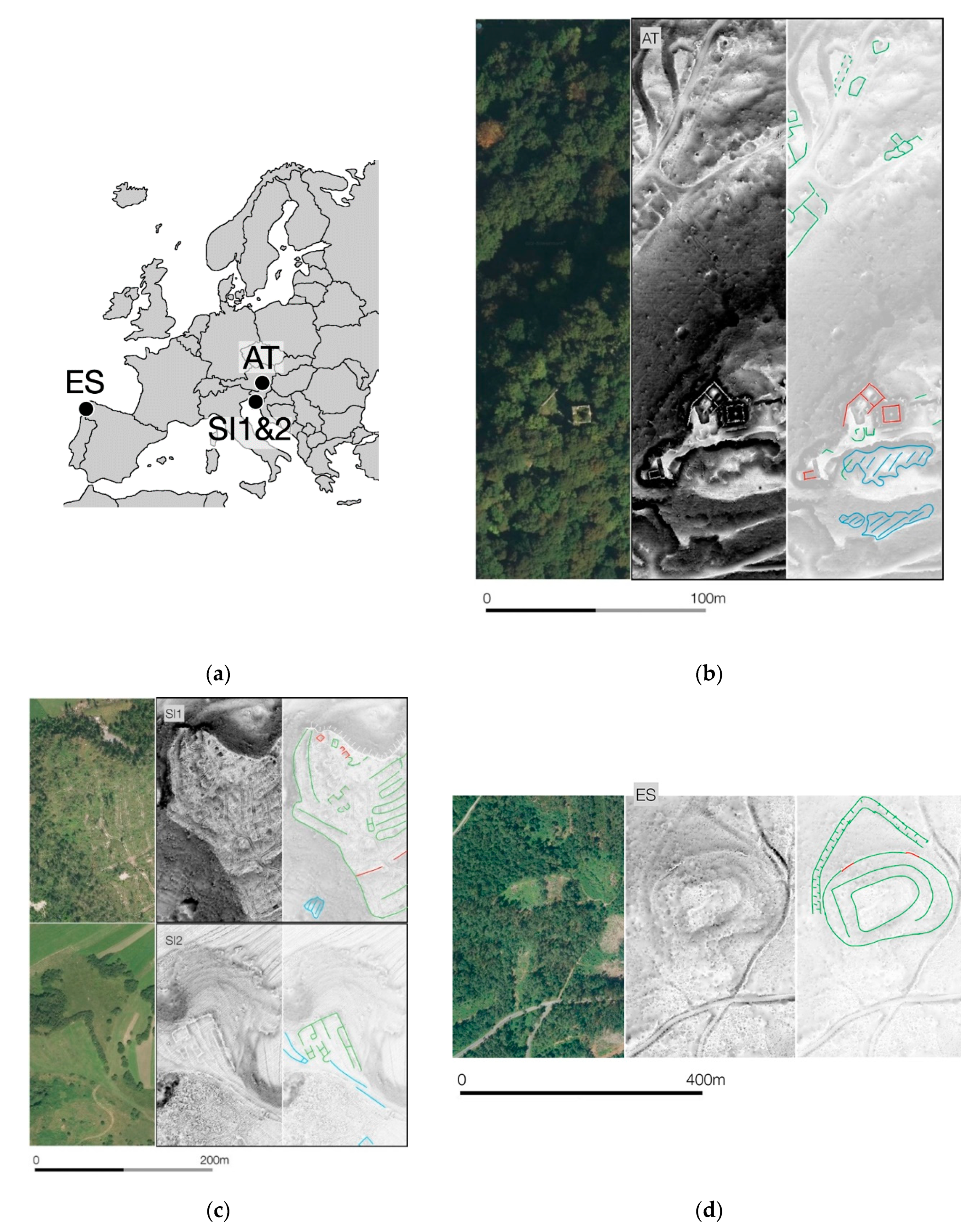
Test sites from Austria (AT), Slovenia (SI), and Spain (ES) were selected based on their archaeological and morphological similarity to compare the filter performance at different point densities. Each site features:
- Hilltop settlement (archaeology)
- Buildings (modern)
- Vegetation on steep slopes
- Sharp discontinuities.
The additional test site (SI2) was chosen for extremely dense vegetation as an example of data with significant gaps in the coverage of the ground points. Each site is 500 × 500 m, but only the most relevant windows are shown in illustrations.
AT airborne LiDAR data was acquired in 2009. These data have a nominal average density of 4 pnt/m2 and an estimated horizontal and vertical root mean square error (RMSE) of 0.15 and 0.40 m, respectively. Ground point filtering is not documented [28]. Point cloud data are available via a formal request (we have acquired the data in the non-classified XYZ format, other formats may be available). The AT test site has 3,844,873 points with an average density of 18.79 pts/m2, which is significantly higher than the nominal average density.
The SI data was acquired in 2014. These data have a nominal density of 5 pnt/m2 and an estimated horizontal and vertical RMSE of 0.09 m. Ground point filtering was performed with the proprietary filter gLidar [29] and is distributed via the eVode WMS (LAS or LAZ format, ISPRS classes 0–7 are populated). The SI1 test site has 2,809,344 points with an average density of 12.28 pts/m2 and the SI2 has 2,756,756 points with an average density of 12.43 pts/m2. It must be mentioned that due to the specific processing of the raw data, each point has a near-double “shadow point”. The “shadow point” is within 0.14 m horizontally and within 0.03 m vertically from the original point, but the distance and bearing to the original is not constant. This means that the functional point density is half of the above-mentioned, namely 6.14 pts/m2.
The ES data was acquired in 2015, with an average density of 1 pnt/m2 and the altimetric accuracy and precision with a RMSE of less than 0.20 m. Ground point filtering is not documented [30]. The point cloud data is distributed by the CNIG Download Center (LAZ format, ISPRS classes 0–7, 10, 12 are populated). The test site ES has 453,255 points with an average density of 1.83 pts/m2.
The most important metadata are summarized in Table 1.
It is not our intention to present the archaeology of the test sites in any detail, but merely to provide the key reference for each archaeological site and to illustrate the archaeological features (Figure 1).
The test site AT is located south of Graz near the town Wildon on a rocky hill consisting of algal limestone and marlstone interspersed with layers of clay that rise above the Mur River valley [31]. It is covered with a dense, mature deciduous forest with little undergrowth. The multiperiod archaeological site Wildoner Schlossberg (N 46°53′05″, E 15°30′48″) is mainly known for two medieval castles and a settlement [32].
The neighboring test sites SI1 and SI2 are located in the Dinaric Karst region named after the Pivka River southwest of Ljubljana. Both sites are located on limestone formations from the Jurassic period, which rise above the karst field Pivška kotlina, known for its intermittent lakes [33]. SI1 is covered by decimated deciduous forest in the first stage of regrowth. It is the site of the prehistoric hillfort Kerin above Pivka (N 45°40′21″, 14°11′40″) [34]. SI2 is characterized by several meadows, each surrounded by very dense deciduous hedges and it is the site of the Roman period villa rustica Sela near Pivka (N 45°40′56″, E 14°12′25″).
Test site ES is located on the magmatic granite hillock midway between the valleys of the Ulla River and its tributary the Vea south of Santiago de Compostela in northwest Spain [35]. It is covered with open deciduous forest and with two small clearings to the east of the site. The archaeological site O Castelo (N 42°44′30″, E 8°33′02″) is a Roman military camp with a probable Iron Age predecessor [36].
On the above mentioned sites 3 out of 4 morphological types of archaeological features are distinguished:
- features embedded in the ground (slight positive or negative bulge, typically up to 0.5 m rise over 5 to 20 m run; blue in Figure 1),
- features partially embedded in the ground (positive or negative spike, typically more than 0.5 m rise over 5 m run; green in Figure 1),
- standing features (an archaeological term for an off-terrain object characterized by a sharp discontinuity in the ground; red in Figure 1), and
- large standing objects (large building-like structures).
Most of the archaeological features detected on airborne LiDAR data fall into the first two types. Examples of type 1 are remains of trenches, ditches, fossil fields, past land divisions, and ancient roads. Examples of type 2 features are dwellings, ramparts, terraces, and burial mounds. Type 3 features occur relatively rarely, mostly as isolated sections of walls (without roof). From the perspective of point cloud filtering, they are non-ground objects. Examples of type 4 features include Mayan monumental architecture at Aguada Fénix, Mexico [5] and Khmer temples in Angkor, Cambodia [7]. These are region specific and are, to our knowledge, not present in European archaeology. Type 4 features are not the subject of this article since they demand additional processing steps that are not accomplished with ground extraction filters.
2.2. Evaluated Filters
We compare all filters known to us that are implemented in an off-the-shelf free or low-cost software under active development or maintenance (Table 2; Appendix A). Accordingly, BCAL Lidar Tools [37] was not considered because its freeware standalone version has been deprecated. Also not considered were legacy Whitebox GAT [38], ALDPAT [39], and LASground [40]. gLiDAR [41,42] was rejected because it was not designed for production and is arguably also legacy program. Furthermore, the skewness balancing filter [43], as implemented in PDAL, was not included because it does not work as intended (in our attempts, all points below a certain height above sea level have been marked as ground and all other as non-ground).
Archaeologists do not typically work with full-waveform airborne LiDAR data (but see [44]), therefore we do not assess post-processing methods for this specific category of airborne LiDAR data in the context of this article.
The analyzed filters are summarized in Table 2.
To our knowledge PMF, SBF, SMRF, CSF, SegBF, and BMHF were not assessed in any of the previous studies [22,23,24,25,26,27].
These and numerous other existing filters are based on algorithms that can be divided into five categories [26,45,46,47]:
- morphological filtering (PMF, SBF, SMRF),
- progressive densification (PTIN),
- surface-based filtering (WLS, CSF),
- segmentation-based filtering (SegBF),
- other (MCC), and
- hybrid (BMHF).
Morphological filtering algorithms are based on the concept of mathematical morphology. They retain terrain details by comparing the elevation of neighboring points [46,47]. A point is classified as ground if its height does not exceed the height of the eroded surface. The filtering is done by two elementary operations: a morphological erosion with the kernel function and a test for the difference between the original height and the eroded height of a point [48].
Progressive densification algorithms work progressively and iteratively classify more and more points as ground by comparing the elevation of the points with the estimated values by different interpolation methods. The initial set of seed ground points is often obtained from the lowest points in a large grid. Ground points are then densified in an iterative process, in which within every triangle the offsets of the candidate points to the triangle surface are analyzed. Points with offsets below the threshold are classified as ground and the algorithm proceeds with the next triangle. The new points are inserted into the triangulation. The process is repeated on the thus densified network until (i) there are no more points in a triangle, (ii) a certain density of ground points is reached, or (iii) when all acceptable points are closer to the surface than a threshold value [26,46,47].
Surface-based filtering algorithms first assume that all points are ground and then gradually remove the points that are not ground. Typically, simple kriging is used in the first step to describe the surface using all points. An averaged surface is then created between the ground and non-ground points. The residual values are created according to their distance from the averaged surface and the points are weighted according to their residual values. Points that have negative residual values are weighted more heavily and are considered ground points. There are many extensions and variants of the surface-based filters [26,46].
Segmentation-based filtering algorithms differ from the above-mentioned ones in that they first form homogeneous segments and then analyze segments rather than individual points. Segmentation can be performed using region-growing techniques, adopting either the normal vector or its change, resulting in either planar or smoothly varying surfaces, respectively. Alternatively, homogeneity can be achieved from height or height change only. The segmentation process has been described by the rationale that every point of a segment can be reached from any other point of the same segment, in the sense that it would be possible for a person to walk along such a path. Many implementations rasterize the data in the process and the segmentation methods are often derived from image processing [46].
Other approaches have also been developed. Some are based on determining a set of features for each point depending on the distribution of neighboring points or as measured features of each point. A decision tree based on machine learning is then often used to classify points based on their feature values. Some methods are based on the slopes or curvatures between points [46].
The filters used in this article and their specific implementation in the software are described in more detail in Appendix A.
When comparing the different categories of algorithms, the following points can be summarized. Morphological filtering invariably impose a tradeoff. The erosion of the ground on steep slopes on the one hand and the inclusion of the non-ground points in flat areas on the other hand has to be balanced on a case-by-case basis. A general advantage of both progressive densification and surface-based algorithms is that the geometric properties of the terrain surface and the point cloud data characteristics are separated to a certain extent. Surface-based algorithms produce more reliable results since they also consider the surface trend, and due to their iterative nature, allow for a better adaptation to the terrain. The segmentation-based algorithms have advantages mostly in urban areas where flat segments are prevailing [46]. Bujan recommends that morphological filtering algorithms are best suited for terrains with small objects, progressive densification for urban areas and terrains with diverse objects, while surface- and segmentation-based algorithms work best in forests and on steep slopes [47]. To this, we may add that one of the key features of segmentation-based algorithms is that the outliers (low and high) theoretically have a limited impact on the result. Thus, they should be suitable to handle data sets with significant noise such as point clouds obtained by structure from motion (SfM).
Nevertheless, all algorithms present similar difficulties when implemented in sharply changing terrain, low vegetation, areas with dense non-ground features, and complicated landscapes [20,46,47,49,50]. The two-decade-old expectation that the fusion of multiple sources (e.g., RGB values or intensity) and integration of different methods will improve the performance [20,51,52] is yet to materialize in off-the-shelf software.
The long-term comparison of the performance of specific algorithms is also reveling. Between 1996 and 2007, uniform algorithms prevailed, with densification being the most important one. Between 2007 and 2012, hybrid algorithms prevailed, and between 2012 and 2016 there was a period of renewed interest in uniform algorithms [47]. Early studies showed that algorithms incorporating a concept of surface performed better than morphological algorithms. In the test environment, a gradual improvement in the performance of algorithms, regardless of the concept they are based on, has been observed in the past two decades [47].
2.3. Method for Quantitative and Qualitative Assessment
Above mentioned studies that have compared relevant filters [22,23,24,25,26,27] used different approaches to calibrating filters with custom settings, which depends strongly on the skillset of the operator. Some omitted calibration by using default settings to minimize the subjective influence of the operator [25]. However, not only are the results more accurate when filters are calibrated, but some filters are also more susceptible to calibration than others [27]. Accordingly, most studies compare calibrated filters [22,23,26]. Our decision to compare calibrated filters was ultimately guided by our search for the best workflow, which must always include calibration.
We have minimized the subjectivity of the calibration process through intensive testing (383 preliminary DTMs were created as a result). For most filters, we used the method of relevant incremental adjustments for each variable, starting with the default value until the best result was found. As the process was guided by experience, in most cases, fewer than 4 attempts were required for each variable. As a typical example is the variable(s) of the MCC, case study AT:
- step 1: default value 2.0;
- step 2: value 3.0 leads to a deterioration;
- step 3: value 1.0 leads to an improvement;
- step 4: value 0.5 leads to a deterioration;
- result: value 1.0 is optimal.
Such an approach was not possible with the SMRF, since out of five variables there are two inversely related pairs. This means that a pair of variables must be changed each time, resulting in almost infinite combinations. Thus, we tested 15 settings that were optimized for ISPRS reference data sets [53].
The 36 best results—9 filters each for AT (Figure 2), SI1 and SI2 (Figure 3), and ES (Figure 4)—were compared qualitatively and quantitatively. The comparison was made by adapting the qualitative and quantitative methods of Sithole and Vosselman [20] for archaeology.
First, we manually classified a point cloud using context knowledge (AT, SI1, and SI2) and aerial photographs. The points were classified into the ground (2) and non-ground (1) using the Global Mapper software package, and only after careful inspection were the classifications accepted.
The qualitative assessment method is defined as a visual examination and comparison of the datasets. Five categories of circumstances in which the algorithms are likely to fail are observed:
- outliers (low or high, occur mainly due to sensor errors);
- object complexity (refers to buildings that are difficult to detect due to their size, low height, or complex shape);
- detached objects (buildings on slopes, bridges, ramps);
- vegetation (problematic categories are vegetation on slopes and low vegetation);
- discontinuity (sharp changes in a slope like cliffs and sharp ridges are treated as buildings).For the purposes of this study, we have added the archaeology-specific category:
- archaeological features (type 1, type 2, and type 3 as defined above in Section 2.1).
Each observed category is rated as good (item is filtered most of the time), fair (item is not filtered a few times), or poor (item is not filtered most of the time). Influence on neighboring points is also rated as good (no influence), fair (small influence), or poor (large influence).
In a similar vein, for the purposes of this study, some of the categories are irrelevant either because all filters perform good (high outliers) or because they are irrelevant to archaeology (object complexity, detached objects). Nevertheless, where present, these categories were still evaluated but are marked in grey.
It should be noted that this method is subjective by design. In this particular case, it has been carried out by two archaeologists who have extensive experience with airborne LiDAR data. It is therefore to be expected that the visual assessment is biased towards the qualities that are archaeology-specific.
The quantitative assessment was done by generating cross-matrices of each generated classified point cloud with the manually classified point cloud. The cross-matrices were then used to evaluate Type I (rejection of bare-Earth points, i.e., false negative) and Type II (acceptance of object points as bare-Earth, i.e., false positive) errors. An example of type I error is when a ground point is classified as non-ground. An example of type II error is when a non-ground point, for example belonging to a building, is classified as ground.
Quantitative assessment was carried out on small areas of 50 × 50 m within archaeological sites. If we were to apply the original method directly, the archaeology-specific accuracy would be masked by the overall accuracy (similar to how low noise was masked in the original study).
The areas were selected according to two criteria:
- the archaeological features must cover at least 50% of the area, and
- the area represents the most difficult rather than average situation.
3. Results
3.1. Qualitative Assessment
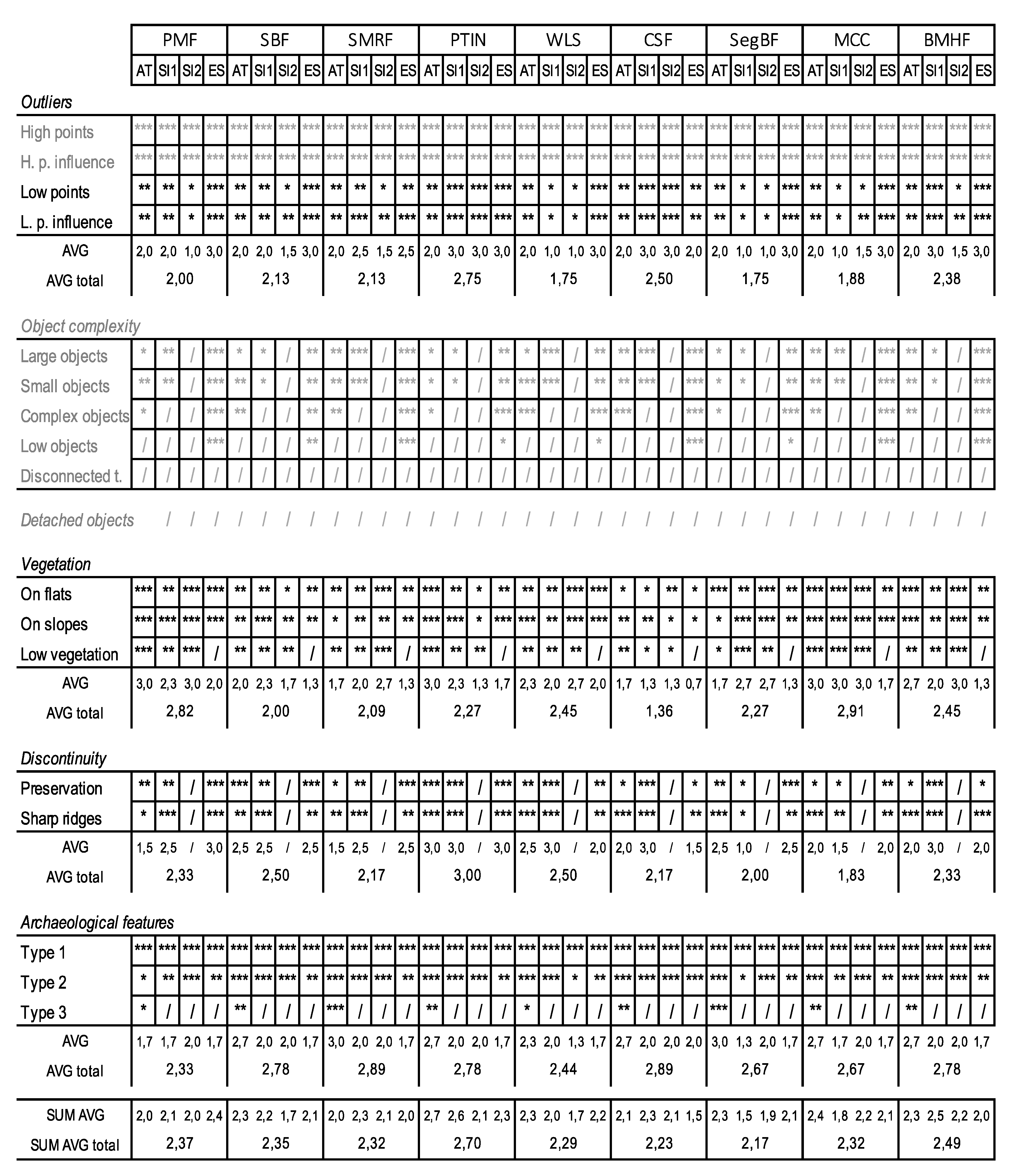
The results of the qualitative assessment are summarized in Figure 5.
The PTIN achieved the highest average, followed by the BMHF, and PMF and SBF. The most robust performers—fewest one—were PTIN and SBF, followed by SMRF and BMHF.
On average, filters performed better on dense data than on medium and low density data. By far the best on dense data was PTIN, followed by MCC and SBF, WLS, SegBF, and BMHF. PTIN and BMHF performed best on medium density data, followed by CSF and SMRF. For low density data, PMF, PTIN, and WLS were the best.
For vegetation removal, MCC was best, followed by PMF and then WLS and BMHF as a distant third. In the preservation of discontinuities, PTIN was perfect, while SBF and WLS were acceptable. In the retention of archaeological features, SMRF and CSF were almost perfect, closely followed by SBF, PTIN, and BMHF.
PTIN was the only filter consistently among the three best; the only comparable was BMHF, which struggled with the preservation of discontinuities and failed almost completely for low-density data.
3.2. Quantitative Assessment
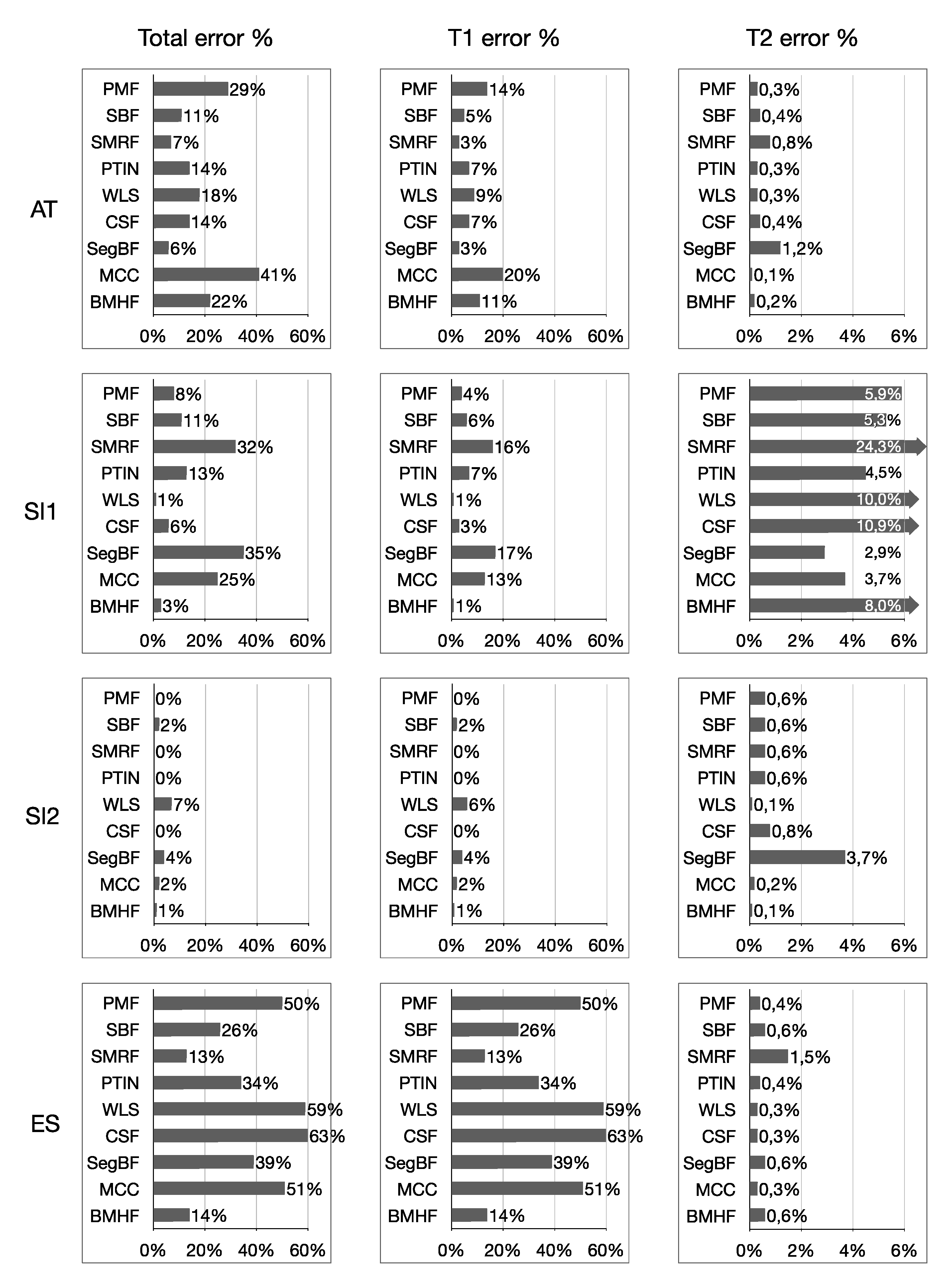
The results of the qualitative assessment are summarized in Figure 6. To facilitate comparison, the performance of each filter in each category was evaluated as follows. The filter with the best performance and the lowest error received nine points, the second-best eight points... the filter with the highest error—the last of nine filters evaluated—received one point. The best score in total error was obtained by SMRF, followed by a close group of BMHF, PTIN, SBF, and CSF. At the bottom of the group were PMF, SegBF, and, at some distance, WLS. The most robust performers were PTIN and BMHF (twice and once second best, respectively; never among the two worst), followed by SBF and CSF (never among the worst). The T1 error results are almost identical to total error.
The T2 error is very different, though. MCC and WLS are decidedly the best, followed by a narrow group of PTIN, BMHF, and PMF. SBF, CSF, SegBF, and at some distance SMRF are the worst.
4. Discussion
The qualitative assessment revealed that some of the categories are irrelevant for this study either because all filters perform good and would only obscure relevant differences (high outliers) or because they are irrelevant to archaeology (detached objects) or are not the subject of this article (object complexity; see archaeological features type 4 in Section 2.1 above). Nevertheless, the results are included in the table where possible (there were no detached objects in our data) to comply with the original method but are omitted from the numerical average.
Extreme examples of very dense vegetation and low vegetation (SI2) remain unsolvable for all filters. Also, the removal of vegetation on steep slopes remains problematic, but with dense data (AT) it is solved well by all filters, as is the discontinuity retention. There is a direct relationship between vegetation on the one hand and archaeology and discontinuity retention on the other hand: the more the vegetation is removed the more of archaeology and discontinuities will be removed as well.
With a few exceptions, all filters have performed well in the retention of archaeological features of types 1 (features embedded in the ground) and 2 (features partially embedded in the ground). However, there are significant differences among the filters in the costs of this retention on the vegetation removal and discontinuity retention. It is not surprising that none of the filters has fully preserved the type 3 features (standing features), as these are by definition off-terrain objects.
The results of the quantitative assessment are not clear-cut. Total error and the T1 error are almost identical, since the T1 error makes up the majority of the total error. The T2 error results are very different and—in the case of MCC, WLS, and SMRF—inverse. The latter can be easily explained: the more ground points classified (lower T1), the more are misclassified (higher T2) and vice versa. This means that MCC and WLS minimize the T2 error at the expense of the high T1 error and SMRF does the opposite. This insight could be exploited in the form of a multi-step hybrid algorithm combining, for example, MSS and SMRF. On their own MCC and WLS are suitable for high and possibly medium-density data, but not for low-density data.
On balance, BMHF and PTIN are notably better than the rest, with SBF and PMF providing acceptable performance.
5. Conclusions
Qualitative and quantitative results are not directly comparable. Thus, no filter is directly better than the rest, but the commercial filters PTIN and BMHF are consistently at the top, followed by an open access SBF. The ability of the MCC to remove vegetation is very good, as is the retention of discontinuities and archaeological features retention of the SBF. Unfortunately the BMHF—which is a hybrid of MCC and SBF—does not succeed in combining the strengths of both.
It is noticeable that in our assessment, filters based on newer algorithms (PMF, CSF, SMRF) are outperformed by some of the oldest (PTIN, SBF), which contradicts recently published findings [46]. This is a reminder of the indirect path from publishing an algorithm to the filter implementation. The latter needs to be refined and optimized, which seems to be best handled by commercial software developers. This insight puts into perspective the purpose of publishing more and more new algorithms that are only compared to the published results, e.g., [47], but are neither implemented as off-the-shelf filters nor compared to them.
Based on the qualitative assessment the archaeology-specific comparison of existing filters can be determined. The qualitative results are directly transferable to real-world problem-solving processes concerning which filter work best for a given combination of data density, landscape type, and type of archaeological features.
Concerning the influence of point density on filter performance, our results are consistent with the results presented by Sithole and Vosselman [20], namely in that the lower the point density, the worse the performance of all filters. This makes processing low-density data much more demanding.
As far as archaeological features are concerned, all filters handle the features embedded in the ground perfectly. Some filters (PMF, WLS, SegBF) struggle with semi-embedded features and all but two (SMRF, SegBF) erase standing features completely. An automatic solution for the handling of standing features has yet to be found. Therefore, a considerable manual classification effort is still inevitable [13,15].
Author Contributions
Conceptualization, B.Š. and E.L.; methodology, B.Š.; formal analysis, E.L.; writing—original draft preparation, B.Š.; writing—review and editing, B.Š.; visualization, E.L.; project administration, B.Š and E.L.; funding acquisition, B.Š. and E.L. All authors have read and agreed to the published version of the manuscript.
Funding
This research was funded by ARRS SLOVENIAN RESEARCH AGENCY, grant numbers N6-0132 and P6-0064, and FWF AUSTRIAN SCIENCE FOUND grant number 13992.
Acknowledgments
The authors thank Stefan Eichert for technical support with PDAL and R software.
Conflicts of Interest
The authors declare no conflict of interest. The funders had no role in the design of the study; in the collection, analyses, or interpretation of data; in the writing of the manuscript, or in the decision to publish the results.
Appendix A. Description of and Experience with the Filters Used in the Case Studies
The descriptions of the filters are based on cited references. The descriptions of the user-facing parameters based on the documentation of the respective software (regular text) are followed by our own archaeology-specific experiences (in italics). All numerical values are given in map units, unless otherwise stated. The exact values used in each of the best results are summarized in Table A1.
Appendix A.1. Morphological Filtering
Appendix A.1.1. PMF
Progressive morphological filter removes the off-ground objects applying elevation difference thresholds in gradually increasing window sizes. However, the implementation is not strict. It works at the point cloud level without any rasterization process, and the morphological operator is applied to the point cloud and not to a raster. Also, the sequence of windows sizes and thresholds is not computed from the original, but is free and user-defined.
Software: lidR 2.2.4 (R-CRAN module), cran.r-project.org.
Price: free.
Algorithm reference: [54].
User-facing parameters:
(ws) Sequence of window sizes: smallest, largest, and step (default: 3,12, 3). Decreasing the smallest window size had no noticeable effect on our results. Increasing the largest window to 18 brought modest improvements in most areas, but it was extremely detrimental to sharp ridges. Therefore, the default settings were used.
(th) Sequence of threshold heights above the parameterized ground surface to be considered as ground return (default: 0.3, 1.5). Decreasing the lower threshold to 0.1 moderately improved all results. The higher threshold had the greatest influence of all parameters; the default value worked best for all of the terrain types other than on the sharpest ridges where entire sections have been misclassified. A value of 3.5 was best compromise with noticeable but tolerable T1 errors on both sharp archaeological features (i.e., ridges of the order of decimetres have their tops cut off) and on the ridges (i.e., ridges of the order of tens of meters have their tops cut off).
Appendix A.1.2. SBF
Slope-based filtering is based on the observation that a large height difference between two nearby points is unlikely to be caused by a steep slope in the terrain. The probability that the higher point could be a ground point decreases as the distance between the two points decreases and an acceptable height difference between two points has been defined as a function of the distance between the points. The inter-point slope threshold and inter-point height threshold must both be exceeded within a given radius for a point to be considered non-ground. SBF filters suffer from the challenge of applying a constant slope threshold to terrain with widely varying slopes.
To mitigate the above-mentioned challenge, this implementation first normalizes the underlying terrain with a white top-hat normalization. Then, points within a given radius that are both (i) above neighboring points by the minimum height threshold and (ii) have an inter-point slope greater than the slope threshold are considered non-ground points.
Software: Whitebox tools (LidarGroundPointFilter), jblindsay.github.io.
Price: free.
Reference: [48].
User-facing parameters:
(r) Search Radius refers to the local neighborhood within which the inter-point slopes are compared (default: 2). Values in correlation with the point cloud density—about 7 times the cell-size of the final DEM—have been used.
(n) The minimum number of neighboring points within the search areas; if fewer points are identified, the search radius is extended until this value is reached or exceeded (default: not set). Value 3 lead to the best results.
(st) Inter-point slope threshold (default: 45 deg). The default value works best for most data sets other than for low-density point clouds, for which value must be significantly decreased.
(ht) Inter-point height threshold (default: 1). Suitable values that do not exceed the default value have been inversely related to the point cloud density.
(n) The slope normalization defines whether initial white top-hat normalization is performed (default: on). Always on.
Appendix A.1.3. SMRF
The simple morphological filter filters point cloud by applying a linearly increasing window and a simple slope thresholding together with an application of image inpainting techniques. First, the lowest point within each cell is retained and empty cells are inpainted. Then a vector of window sizes (radii) is generated and gradually increased to the supplied maximum value. For each window, an elevation threshold value is generated that corresponds to a supplied slope parameter and is multiplied by the product of this window size and the cell size of the minimum surface grid. Based on the latter, a surface is generated using a disk-shaped element with a radius equal to the current window size. At each step, each cell is classified as a ground point if the difference between the current and previous surface is greater than the calculated elevation threshold. In an additional process, low outliers are removed. The application is not strict.
Software: PDAL 2.1.x, pdal.io.
Price: free.
Reference: [53].
User-facing parameters:
(c) Cell size of the minimum surface grid (default: 1). The default value was used.
(sc) The elevation scalar parameter assists in the identification of ground points from the provisional DEM; it is inversely related to the scaling factor (default: 1.25). Values between 0 and 1.5 were used, values around 1.5 were optimal for dense data of forested steep slopes with very sharp edges.
(st) The slope threshold value controls the process of ground/non-ground identification at each step and should approximate the maximum slope of the terrain; it’s inversely related to the maximum window radius (default: 0.15 rise over run). Values between 0.05 and 0.28 were used, on average ½ of the steepest slope; the lowest value was used for low-density data.
(w) The maximum window radius controls the opening operation at each iteration and corresponds to the size of the largest feature to be removed. This is inversely related to the slope threshold (default: 18.0). Predominantly values between 15 and 20 were used.
(t) The elevation threshold determines the final classification of the point as ground/non-ground based on the interpolated vertical distance from the minimum surface grid. This is inversely related to the scaling factor (default: 0.5). Values between 0.25 and 0.5 were used.
General note: the interconnectedness of parameters makes the search for optimal settings very time-consuming. Our approach was to test 15 optimal combinations of settings developed for the ISPRS reference data sets by Pingel et al. [53].
Appendix A.2. Progressive Densification
PTIN
The progressive triangulated irregular network algorithm, sometimes referred to as the Axelsson algorithm, first generates a sparse TIN from seed points. It is then densified in an iterative process by including the returns according to their distance from the TIN facets and their angles to the nodes. The TIN adapts to the data points from below and is limited in its curvature by parameters derived from the data. The algorithm is designed to handle surfaces with discontinuities, such as dense city areas.
This is a non-strict implementation (cf. Štular, Lozić 2016; Pfeifer, Mandlburger 2018) and the details are not published. The user-facing parameters reveal at least two steps in addition to the original algorithm: spike and bulge removal.
Software: LAStools (LASground_new), rapidlasso.com.
Price: 1500–3000€ or more.
Reference: [55].
User-facing parameters:
(st) Step size defines the size of the initial search window, which depends on the roughness of the terrain (default: 25).
(g) Granularity refers to the intensification of the search for initial ground points; higher values are recommended for steeper slopes (default: 5.0).
(off) Offset is a measurement up to which points above the current ground estimates are included (default: 0.05).
(s) Spike is the threshold at which positive and negative spikes are removed (default: spike-down 1).
(b) Bulge refers to the curvature by which the TIN is constrained when fitted to the data points (default is set to a tenth of the step size and then clamped into the range from 1.0 to 2.0).
One of the biggest advantages of this implementation compared to all others is the presets for the user-facing parameters. The step size presets are described in terms of terrain types (metro, city, town, nature, and wilderness; 50, 25, 10, 5, and 3 respectively). The granularity is described in terms of pre-processing (coarse, default, fine, extra-fine, ultra-fine, hyper-fine). Wilderness in combination with Hyper-fine works best for dense point clouds (AT, SI1&2), Nature in combination with Fine for low-density point clouds (ES). In data with low-noise (SI1&2), down-spike 0.75 largely removes the low noise.
Appendix A.3. Surface-Based Filtering
Appendix A.3.1. WLS
The weighted linear least-squares interpolation first generates an initial surface that lies between the true ground and the canopy. It is more likely that terrain points are below and vegetation points are above the initial surface. The distance and direction to the surface is then used to calculate weights for each point based on linear prediction with an individual accuracy for each measurement, i.e., the probability for each point to be either ground or non-ground. The process is repeated. The implementation is an adaptation of the Kraus and Pfeifer algorithm.
Software implementation: Fusion 3.80, ground filter v 1.81, forsys.cfr.washington.edu/FUSION.
Price: free.
User-facing parameters:
(c) Cell size used for intermediate surface models (default: 10). Double the cell-size of the final DEM worked best.
(gparam) The G-parameter value of the weight equation determines the distance from the surface at which points are automatically defined as ground (default: −2.0). Negligible improvements have been achieved by using the value to 0 (in combination with increasing the number of iterations).
(wparam) The W-parameter value of the weight equation (default: 2.5). Negligible improvements were achieved by reducing the value to 0.5 (in combination with the increase of the iterations).
(it) Number of iterations for the filtering logic (default: 5 iterations). Increasing the number of iterations up to 10 resulted in a moderate reduction of T2 errors, an increase beyond that resulted in negligible improvements; increasing the number of iterations extends the processing time linearly.
(olh) Outlier: low, high omit points with height above ground below low and above high. Our tests did not show any noteworthy positive effect on low noise removal or otherwise.
(t) Tolerance to the final surface for the points to be considered ground/non-ground (by default, the weight value is used to filter the points). No improvements have been achieved, the use of default weight is recommended.
(fs) Final smooth refers to a slightly more aggressive smoothing of the intermediate surface model just before the final point selection process. Not to be used for archaeology.
Other switches (smooth, aparam, bparam) are not intended for use in a production environment.
Appendix A.3.2. CSF
Cloth simulation filter is based on a 3D computer graphics algorithm that is used to simulate cloth. First, a LiDAR point cloud is inverted and then a rigid cloth is used to cover the inverted surface. By analyzing the interaction between the cloth nodes and the corresponding LiDAR points, the locations of the cloth nodes are determined and used to generate an approximation of the ground surface. Finally, the ground points can be extracted from the point cloud by comparing the original points with the generated surface. All software implementations are strict.
Software implementation: CloudCompare 2.10.2, www.danielgm.net/cc/, CSF plugin (also available in R and PDAL).
Price: free.
Algorithm reference: [58].
User-facing parameters:
(s) Scene: the rigidness of the cloth is determined; very soft to fit steep slope, medium for rugged terrain, and hard cloth for flat terrain (default: medium). No discernible differences between very soft and medium were observed, hard was not suitable.
(r) Cloth resolution: refers to the grid size of the cloth with which the terrain is covered, i.e., the distance between the particles in the cloth (default: 2.0). The same value as the resolution of the final DEM worked best, lower values (e.g., ½ the cell-size of the final DEM) introduced artifacts. Lowering the value increases the processing times exponentially.
(it) Max. Iterations: maximum iterations for the cloth simulation (default: 500 iterations). A significant increase of the iterations (max. value 1000) produced modest improvements at the expense of a linear increase of the processing time.
(th) Classification threshold: the distance to the simulated cloth to classify a point cloud into ground and non-ground (default: 0.5). On flat terrain lower values (e.g., 0.15) slightly reduced T2 error, but on average or rugged terrain the default value is recommended.
(sp) Slope processing: reduces errors during post-processing when steep slopes are present (default: off). Switching on significantly improved handling of cliffs and low walls, but resulted in noticeable T2 errors, e.g., “tree stumps” on slopes and buildings on the flats.
Appendix A.4. Segmentation Based Filtering
SegBF
A segmentation based filter identifies ground points using a segmentation based approach that builds on the assumption that the largest segment in any airborne LiDAR dataset is the ground surface. In particular, this approach uses the random sample consensus (RANSAC) method to identify points within a point cloud that belong to planar surfaces, which means that the segmentation is performed using region-growing techniques using normal vectors that result in planar surfaces.
In this implementation, the algorithm begins by attempting to fit the planar surfaces to all points within a user-defined radius. The planar equation is stored for each point for which a suitable planar model can be fitted. A region-growing algorithm is then used to match nearby points with similar planar models. The similarity is based on a maximum allowable angular difference between the plane normal vectors of the two neighboring points. Segment edges for ground points are determined by a maximum allowable height difference between neighboring points on the same plane.
Software: Whitebox tools (LidarSegmentationBasedFilter), jblindsay.github.io.
Price: free.
User-facing parameters:
(r) Search radius, within which planar surfaces are fitted (default: 5). Lower values than the default worked best without correlation to either point density or terrain type; increasing values lengthen the processing time exponentially.
(s) Maximum difference of normal vectors considered for similarity (default: 2 deg). Values between 1 and 2 worked best without correlation to point density or terrain type.
(h) Maximum difference in elevation between neighboring points in the same segment (default: 1). In all but one case, the value 0.5 worked best.
General note: in our best results there is a direct correlation between (r) and (s): (s) ≈ ½ (r).
Appendix A.5. Other Filters
Appendix A.5.1. MCC
The multiscale curvature classification of ground points in airborne LiDAR point clouds iteratively classifies non-ground points that exceed positive curvature thresholds on multiple scales. It uses thin-plate spline interpolation to generate surfaces at different resolutions and uses progressive curvature tolerances to eliminate non-ground returns. During processing, the scale and initial curvature are changed over three domains to account for variable canopy configurations and their interaction with terrain slope: the initial value set to scale is multiplied by 0.5, 1, and 1.5, while 0.1 is added to the initial curvature in each domain. The software implementation is strict.
Software implementation: MCC-LIDAR 2.2, sourceforge.net/projects/mcclidar.
Price: free.
Algorithm references: [61].
User-facing parameters:
(λ) The scale refers to the size of the search window used for the interpolation of the points (default: 1.5). Values between 1.0 and 2.0 worked best, so the default value is an excellent start for experimenting.
(t) Minimum height deviation from the interpolated surface for non-ground point (default: 0.3). Values between 0.2 and 0.25 worked best, which means that the default value might be set slightly too high for archaeology.
Appendix A.5.2. BMHF
Blue Marble Geographic’s hybrid filter is a two-part process that first removes points that are likely not ground and then compares the remaining points to a modeled curved 3D surface within a window. This is an implementation of MCC that uses SBF for pre-processing to speed up the processing significantly.
Software: Global Mapper 21.x, bluemarblegeo.com
Price: 1098$.
Reference: bluemarblegeo.com.
User-facing parameters:
(ht) Maximum height delta refers to the expected elevation range of the ground in the point cloud (default: 50). Default value worked best for all datasets.
(st) Expected Terrain Slope, i.e., threshold value for the inter-point slope (default: 7.5 deg). Higher values worked best for dense datasets with steep slopes, lower values were used for low-density data sets and the lowest value for flat terrain.
(b) Maximum width of buildings; large values cause longer processing times (default: 100). Values between 10 and 25 worked well, but since this is an iterative process—larger values remove big and small buildings—the default value is recommended.
(bin) Base bin size refers to the size of the search window size that is used to interpolate the points and can be set either in meters or in points (average is calculated for the loaded data; default: 3 points). Default value 3 points worked vel; the value in meters is recommended when reproducible results are needed across different data sets; often 3 times the value of the final DEM cell-size worked best.
(h) Minimum height deviation from the interpolated surface for non-ground points; larger values (such as 1 to 3) are necessary for low-density point clouds (default: 0.3). The default value worked best in all data sets.

Table A1.
Values used in each of the best results.
| Tested Settings | Best Settings | |||||||
|---|---|---|---|---|---|---|---|---|
| Setting | Range | Step | AT | SI1 | SI2 | ES | ||
| PMF | ws | 3,12, 3 | 3,18, 3 | 3 | 3,12, 3 | 3,12, 3 | 3,12, 3 | 3,18, 3 |
| th | 0.1, 1.0 | 0.3, 7.0 | 0.5 (0.2 1) | 0.1, 7.0 | 0.3, 1.5 | 0.3, 1.5 | 0.1, 1.0 | |
| SBF | r | 2.0 | 7.5 | 0.5 | 2.0 | 3.0 | 3.0 | 7.5 |
| n | 3 | 3 | 1 | 3 | 3 | 3 | 3 | |
| st | 25 | 60 | 5 | 60 | 45 | 30 | 25 | |
| ht | 0.3 | 1.0 | 0.5 (0.2 1) | 1 | 0.5 | 0.5 | 0.3 | |
| n | on | on | / | on | on | on | on | |
| SMRF | c | 1.0 | 1.0 | / | 1.0 | 1.0 | 1.0 | 1.0 |
| sc | 0.0 | 1.45 | / | 1.45 | 1.3 | 0.0 | 0.9 | |
| st | 0.05 | 0.28 | / | 0.28 | 0.16 | 0.12 | 0.05 | |
| t | 0.35 | 0.45 | / | 0.45 | 0.35 | 0.45 | 0.35 | |
| w | 5 | 20 | / | 5 | 18 | 20 | 17 | |
| PTIN | st | 3 | 10 | / | 5 | 3 | 5 | 10 |
| g | / | / | / | / | / | / | / | |
| off | 0.05 | 0.5 | 0.05 | 0.05 | 0.05 | 0.05 | 0.05 | |
| s+ | 0.5 | 2.0 | 0.25 | 1.0 | 1.0 | 1.0 | 1.0 | |
| s- | 0.5 | 2.0 | 0.25 | 1.0 | 0.75 | 0.75 | 1.0 | |
| b | / | / | / | no | no | no | no | |
| terrain type | wilderness | city | / | wilderness | nature | wilderness | town | |
| pre-processig | Hyper-fine | fine | / | ultra fine | hyper fine | ultra fine | ultra fine | |
| WLS | c | 0.25 | 3 | 0.5 (0.25) | 0.5 | 1 | 1 | 2 |
| gparam | −3.0 | 0.5 | 0.5 | 0 | 0 | −1.0 | 0 | |
| wparam | 0.5 | 3.0 | 0.5 | 0.5 | 0.5 | 0.5 | 0.5 | |
| olh | 0 | 2 | 0.5 | No | No | No | No | |
| it | 2 | 20 | 5 | 10 | 10 | 10 | 10 | |
| fs | No | Yes | / | No | No | No | No | |
| CSF | s | hard | med | / | hard | hard | hard | medium |
| r | 0.3 | 1 | 0.5 (0.2 1) | 0.3 | 0.5 | 0.5 | 1 | |
| it | 1000 | 1000 | 250 | 1000 | 1000 | 1000 | 1000 | |
| th | 0.5 | 0.5 | 0.5 (0.2 1) | 0.5 | 0.5 | 0.5 | 0.5 | |
| sp | on | on | / | on | on | on | on | |
| SegBF | r | 1.5 | 4.5 | 0.5 | 4.5 | 1.5 | 1.5 | 3.0 |
| s | 1.0 | 2.0 | 0.5 | 2.0 | 1.0 | 1.0 | 1.5 | |
| h | 0.25 | 0.5 | 0.25 | 0.5 | 0.5 | 0.25 | 0.5 | |
| MCC | λ | 0.5 | 2.5 | 0.25 | 1.0 | 2.0 | 2.0 | 1.75 |
| t | 0.1 | 1.0 | 0.1 | 0.2 | 0.2 | 0.2 | 0.2 | |
| BMHF | ht | 25 | 100 | 25 | 50 | 50 | 50 | 50 |
| st | 5 | 40 | 2.5 | 35 | 35 | 7.5 | 15 | |
| b | 5 | 30 | 5 | 20 | 25 | 10 | 20 | |
| bin | 0.5 | 2.0 | 0.25 | 0.75 | 1.5 | 1.5 | 3 | |
| h | 0.1 | 0.5 | 0.1 | 0.3 | 0.3 | 0.3 | 0.3 | |
1 For values under 0.5.
References
- Cohen, A.; Klassen, S.; Evans, D. Ethics in Archaeological Lidar. J. Comput. Appl. Archaeol. 2020, 3, 76–91. [Google Scholar] [CrossRef]
- Chase, A.; Chase, D.; Chase, A. Ethics, new colonialism, and lidar data: A decade of lidar in Maya archaeology. J. Comput. Appl. Archaeol. 2020, 3, 51–62. [Google Scholar] [CrossRef]
- Crutchley, S. Light Detection and ranging (lidar) in the Witham Valley, lincolnshire: An assessment of new remote sensing techniques. Archaeol. Prospect. 2006, 13, 251–257. [Google Scholar] [CrossRef]
- Challis, K.; Carey, C.; Kincey, M.; Howard, A.J. Assessing the preservation potential of temperate, lowland alluvial sediments using airborne lidar intensity. J. Archaeol. Sci. 2011, 38, 301–311. [Google Scholar] [CrossRef]
- Inomata, T.; Triadan, D.; López, V.A.V.; Fernandez-Diaz, J.C.; Omori, T.; Bauer, M.B.M.; Hernández, M.G.; Beach, T.; Cagnato, C.; Aoyama, K.; et al. Monumental architecture at Aguada Fénix and the rise of Maya civilization. Nature 2020, 582, 530–533. [Google Scholar] [CrossRef] [PubMed]
- Stanton, T.W.; Ardren, T.; Barth, N.C.; Fernandez-Diaz, J.C.; Rohrer, P.; Meyer, D.; Miller, S.J.; Magnoni, A.; Pérez, M. “Structure” density, area, and volume as complementary tools to understand Maya Settlement: An analysis of lidar data along the great road between Coba and Yaxuna. J. Archaeol. Sci. Rep. 2020, 29, 102178. [Google Scholar] [CrossRef]
- Evans, D. Airborne laser scanning as a method for exploring long-term socio-ecological dynamics in Cambodia. J. Archaeol. Sci. 2016, 74, 164–175. [Google Scholar] [CrossRef] [Green Version]
- Laharnar, B.; Lozić, E.; Štular, B. A structured Iron Age landscape in the hinterland of Knežak, Slovenia. In Rural Settlement: Relating Buildings, Landscape, and People in the European Iron Age; Cowley, D.C., Fernández-Götz, M., Romankiewicz, T., Wendling, H., Eds.; Sidestone Press: Leiden, Holland, 2019; pp. 263–272. [Google Scholar]
- Gheyle, W.; Stichelbaut, B.; Saey, T.; Note, N.; Van den Berghe, H.; Van Eetvelde, V.; Van Meirvenne, M.; Bourgeois, J. Scratching the surface of war. Airborne laser scans of the Great War conflict landscape in Flanders (Belgium). Appl. Geogr. 2018, 90, 55–68. [Google Scholar] [CrossRef]
- Doneus, M.; Kühtreiber, T. Airborne laser scanning and archaeological interpretation–bringing back the people. In Interpreting Archaeological Topography. Airborne Laser Scanning, 3D Data and Ground Observation; Opitz, R.S., Cowley, D.C., Eds.; Oxbow Books: Oxford, UK, 2013; pp. 33–50. [Google Scholar]
- Crutchley, S.; Crow, P. The Light Fantastic: Using Airborne Laser Scanning in Archaeological Survey; English Heritage: Swindon, UK, 2010. [Google Scholar]
- Doneus, M.; Briese, C. Airborne laser scanning in forested areas–potential and limitations of an archaeological prospection technique. In Remote Sensing for Archaeological Heritage Management, Proceedings of the 11th EAC Heritage Management Symposium, Reykjavik, Iceland, 25–27 March 2010; Cowley, D., Ed.; Archaeolingua: Budapest, Hungary, 2011; pp. 53–76. [Google Scholar]
- Opitz, R.S. An overview of airborne and terrestrial laser scanning in archaeology. In Airborne Laser Scanning, 3D Data and Ground Observation; Opitz, R.S., Cowley, D.C., Eds.; Oxbow Books: Oxford, UK, 2013; pp. 13–31. [Google Scholar]
- Fernandez-Diaz, J.; Carter, W.; Shrestha, R.; Glennie, C. Now you see it... now you don’t: Under- standing airborne mapping LiDAR collection and data product generation for archaeological research in Mesoamerica. Remote Sens. 2014, 6, 9951–10001. [Google Scholar] [CrossRef] [Green Version]
- Štular, B.; Lozić, E. Primernost podatkov projekta Lasersko skeniranje Slovenije za arheološko interpretacijo: Metoda in študijski primer (The Suitability of Laser Scanning of Slovenia Data for Archaeological Interpretation: Method and a Case Study). In Digitalni Podatki; Ciglič, R., Geršič, M., Perko, D., Zorn, M., Eds.; Geografski inštitut Antona Melika ZRC SAZU: Ljubljana, Slovenia, 2016; pp. 157–166. [Google Scholar]
- Doneus, M.; Mandlburger, G.; Doneus, N. Archaeological ground point filtering of airborne laser scan derived point-clouds in a difficult mediterranean environment. J. Comput. Appl. Archaeol. 2020, 3, 92–108. [Google Scholar] [CrossRef] [Green Version]
- Johnson, K.M.; Ouimet, W.B. An observational and theoretical framework for interpreting the landscape palimpsest through airborne LiDAR. Appl. Geogr. 2018, 91, 32–44. [Google Scholar] [CrossRef]
- Rutkiewicz, P.; Malik, I.; Wistuba, M.; Osika, A. High concentration of charcoal hearth remains as legacy of historical ferrous metallurgy in southern Poland. Quat. Int. 2019, 512, 133–143. [Google Scholar] [CrossRef]
- Pingel, T.J.; Clarke, K.; Ford, A. Bonemapping: A LiDAR processing and visualization technique in support of archaeology under the canopy. Cartogr. Geogr. Inf. Sci. 2015, 41 (Suppl. S1), 18–26. [Google Scholar] [CrossRef]
- Sithole, G.; Vosselman, G. Experimental comparison of filter algorithms for bare-earth extraction from airborne laser scanning point clouds. ISPRS J. Photogramm. Remote Sens. 2004, 59, 85–101. [Google Scholar] [CrossRef]
- Lieskovský, T.; Chalachanová, J.F. The assessment of the chosen LiDAR data sources in Slovakia for the archaeological spatial analysis. In Advances and Trends in Geodesy, Cartography and Geoinformatics II; Molčíková, S., Hurčiková, V., Blišťan, P., Eds.; CRC Press: Boca Raton, FL, USA, 2020; pp. 190–195. [Google Scholar]
- Podobnikar, T.; Vrečko, A. Digital elevation model from the best results of different filtering of a LiDAR point cloud. Trans. GIS 2012, 16, 603–617. [Google Scholar] [CrossRef]
- Julge, K.; Ellmann, A.; Gruno, A. Performance analysis of freeware filtering algorithms for determining ground surface from airborne laser scanning data. J. Appl. Remote Sens. 2014, 8. [Google Scholar] [CrossRef]
- Montealegre, A.L.; Lamelas, M.T.; de la Riva, J. A Comparison of Open-Source LiDAR Filtering Algorithms in a Mediterranean Forest Environment. J. Sel. Top. Appl. Earth Obs. Remote Sens. 2015, 8, 4072–4085. [Google Scholar] [CrossRef] [Green Version]
- Andrade, M.S.; Gorgens, E.B.; Reis, C.R.; Cantinho, R.Z.; Assis, M.; Sato, L.; Ometto, J.P.H.B. Airborne laser scanning for terrain modeling in the Amazon forest. Acta Amaz. 2018, 48, 271–279. [Google Scholar] [CrossRef]
- Suleymanoglu, B.; Soycan, M. Comparison of filtering algorithms used for DTM production from airborne lidar data: A case study in Bergama, Turkey. Geod. Vestn. 2019, 63, 395–414. [Google Scholar] [CrossRef]
- Cosenza, D.N.; Pereira, L.G.; Guerra-Hernández, J.; Pascual, A.; Soares, P.; Tomé, M. Impact of calibrating filtering algorithms on the quality of LiDAR-derived DTM and on forest attribute estimation through area-based approach. Remote Sens. 2020, 12, 918. [Google Scholar] [CrossRef] [Green Version]
- Die Steiermark ist komplett... (ALS-Daten). Available online: https://web.archive.org/web/20200908101053/https://www.landesentwicklung.steiermark.at/cms/beitrag/11905526/142970647/ (accessed on 8 September 2020).
- Čekada, M.T.; Bric, V. Končan je projekt laserskega skeniranja Slovenije. Geod. Vestn. 2015, 59, 586–592. [Google Scholar]
- PNOA LiDAR. Available online: https://web.archive.org//web/20200910132414/https://pnoa.ign.es/el-proyecto-pnoa-lidar (accessed on 8 September 2020).
- Gutjahr, C.; Karl, S.; Obersteiner, G.P. Hengist Best-of. Führer zu archäologischen Fundstellen und Baudenkmalen in der Region Hengist; Hengist-Magazin Sonderband 1/2018; Kulturpark Hengist: Wildon, Austria, 2018. [Google Scholar]
- Fuchs, G. Die höhensiedlungen der steiermark im kontext der regionalen siedlungsstrukturen. In Wirtschaft, Macht und Strategie. Höhensiedlungen und ihre Funktionen in der Ur-und Frühgeschichte; Krenn-Leeb, A., Ed.; Verlag Osterreichische Gesellschaft fur Ur- und Fruhgeschichte: Wien, Austria, 2006; pp. 173–187. [Google Scholar]
- Stepišnik, U. Dinarski kras: Plitvi kras Zgornje Pivke; Univerza v Ljubljani: Ljubljana, Slovenia, 2017. [Google Scholar]
- Laharnar, B.; Lozić, E.; Miškec, A. Gradišče above Knežak. In Minor Roman Settlements in Slovenia; Horvat, J., Lazar, I., Gaspari, A., Eds.; ZRC Publishing: Ljubljana, Slovenia, 2020; pp. 123–140. [Google Scholar] [CrossRef]
- Arias, J.G. Mapa Geologico de España. E.1:50.000-Hoja 120–Padrón; Instituto Geológico y Minero de España: Madrid, Spain, 1981. [Google Scholar]
- Costa-García, J.M.; Fonte, J.; Gago, M. The reassessment of the Roman military presence in Galicia and Northern Portugal through digital tools: Archaeological diversity and historical problems. Mediterr. Archaeol. Archaeom. 2019, 19, 17–49. [Google Scholar] [CrossRef]
- BCAL Lidar Tools. Available online: https://web.archive.org/web/20200908101726/https://www.boisestate.edu/bcal/tools-resources/bcal-lidar-tools/ (accessed on 8 September 2020).
- Whitebox Geospatial Analysis Tools. Available online: https://web.archive.org/web/20200908101926/https://jblindsay.github.io/ghrg/Whitebox/ (accessed on 8 September 2020).
- Zhang, K.; Cui, Z. Airborne LiDAR Data Processing and Analysis Tools—ALDPAT 1.0 Software Manual; International Hurricane Research Centre, Department of Environmental Studies, Florida International University: Miami, FL, USA, 2007. [Google Scholar]
- Lasground. Available online: https://web.archive.org/web/20200908102857/https://rapidlasso.com/lastools/lasground/ (accessed on 8 September 2020).
- Mongus, D.; Lukač, N.; Žalik, B. Ground and building extraction from LiDAR data based on differential morphological profiles and locally fitted surfaces. ISPRS J. Photogramm. Remote Sens. 2014, 93, 145–156. [Google Scholar] [CrossRef]
- gLIDAR. Available online: https://web.archive.org/web/20200908103254/https://gemma.feri.um.si/gLiDAR/ (accessed on 8 September 2020).
- Bartels, M.; Wei, H. Threshold-free object and ground point separation in LIDAR data. Pattern Recognit. Lett. 2010, 31, 1089–1099. [Google Scholar] [CrossRef]
- Doneus, M.; Briese, C.; Fera, M.; Janner, M. Archaeological prospection of forested areas using full-waveform airborne laser scanning. J. Archaeol. Sci. 2008, 35, 882–893. [Google Scholar] [CrossRef]
- Briese, C. Extraction of digital terrain models. In Airborne and Terrestrial Laser Scanning; Vosselman, G., Maas, H.-G., Eds.; Whittles Publishing: Dunbeath, UK, 2010; pp. 135–167. [Google Scholar]
- Pfeifer, N.; Mandlburger, G. LiDAR data filtering and digital terrain model generation. In Topographic Laser Ranging and Scanning: Principles and Processing; Shan, J., Toth, C.K., Eds.; CRC Press: Boca Raton, FL, USA, 2018; pp. 349–378. [Google Scholar]
- Buján, S.; Cordero, M.; Miranda, D. Hybrid overlap filter for LiDAR point clouds using free software. Remote Sens. 2020, 12, 1051. [Google Scholar] [CrossRef] [Green Version]
- Vosselman, G. Slope based filtering of laser altimetry data. Int. Arch. Photogramm. Remote Sens. 2000, 33, 935–942. [Google Scholar]
- Meng, X.; Currit, N.; Zhao, K. Ground filtering algorithms for airborne LiDAR data: A review of critical issues. Remote Sens. 2010, 2, 833–860. [Google Scholar] [CrossRef] [Green Version]
- Chen, Z.; Gao, B.; Devereux, B. State-of-the-art: DTM generation using airborne LIDAR data. Sensors 2017, 17, 150. [Google Scholar] [CrossRef] [Green Version]
- Ackermann, F. Airborne laser scanning—Present status and future expectations. ISPRS J. Photogramm. Remote Sens. 1999, 54, 64–67. [Google Scholar] [CrossRef]
- Axelsson, P. Processing of laser scanner data—Algorithms and applications. ISPRS J. Photogramm. Remote Sens. 1999, 54, 138–147. [Google Scholar] [CrossRef]
- Pingel, T.J.; Clarke, K.C.; McBride, W.A. An improved simple morphological filter for the terrain classification of airborne LIDAR data. ISPRS J. Photogramm. Remote Sens. 2013, 77, 21–30. [Google Scholar] [CrossRef]
- Zhang, K.; Chen, S.-C.; Whitman, D.; Shyu, M.-L.; Yan, J.; Zhang, C. A progressive morphological filter for removing nonground measurements from airborne LIDAR data. IEEE Trans. Geosci. Remote Sens. 2003, 41, 872–882. [Google Scholar] [CrossRef] [Green Version]
- Axelsson, P. DEM generation from laser scanner data using adaptive tin models. Int. Arch. Photogramm. Remote Sens. 2000, 33, 110–117. [Google Scholar]
- Kraus, K.; Pfeifer, N. Determination of terrain models in wooded areas with airborne laser scanner data. ISPRS J. Photogramm. Remote Sens. 1998, 53, 193–203. [Google Scholar] [CrossRef]
- McGaughey, R.J. FUSION/LDV: Software for LIDAR Data Analysis and Visualization, v. 3.60; United States Department of Agriculture: Seattle, WA, USA, 2016. [Google Scholar]
- Zhang, W.; Qi, J.; Wan, P.; Wang, H.; Xie, D.; Wang, X.; Yan, G. An easy-to-use airborne LiDAR data filtering Method based on cloth simulation. Remote Sens. 2016, 8, 501. [Google Scholar] [CrossRef]
- Fischler, M.A.; Bolles, R.C. Random sample consensus: A paradigm for model fitting with applications to image analysis and automated cartography. Commun. ACM 1981, 24, 381–395. [Google Scholar]
- Lindsay, J.B.; Francioni, A.; Cockburn, J.M.H. LiDAR DEM smoothing and the preservation of drainage features. Remote Sens. 2019, 11, 1926. [Google Scholar] [CrossRef] [Green Version]
- Evans, J.S.; Hudak, A.T. A multiscale curvature algorithm for classifying discrete return lidar in forested environments. IEEE Trans. Geosci. Remote Sens. 2007, 45, 1029–1038. [Google Scholar] [CrossRef]
Figure 1.
Archaeological features mapped according to morphological types (type 1 embeded features—blue, type 2 partially embeded features—green, type 3 standing features—red). Only the most relevant windows are shown for each test site at 100% crop size: (a) Location of test sites; (b) Test site AT); (c) Test sites SI1 and SI2; (d) Test site ES. DFM is visualized with sky view factor (16 search direction, search radius 10 pixels).

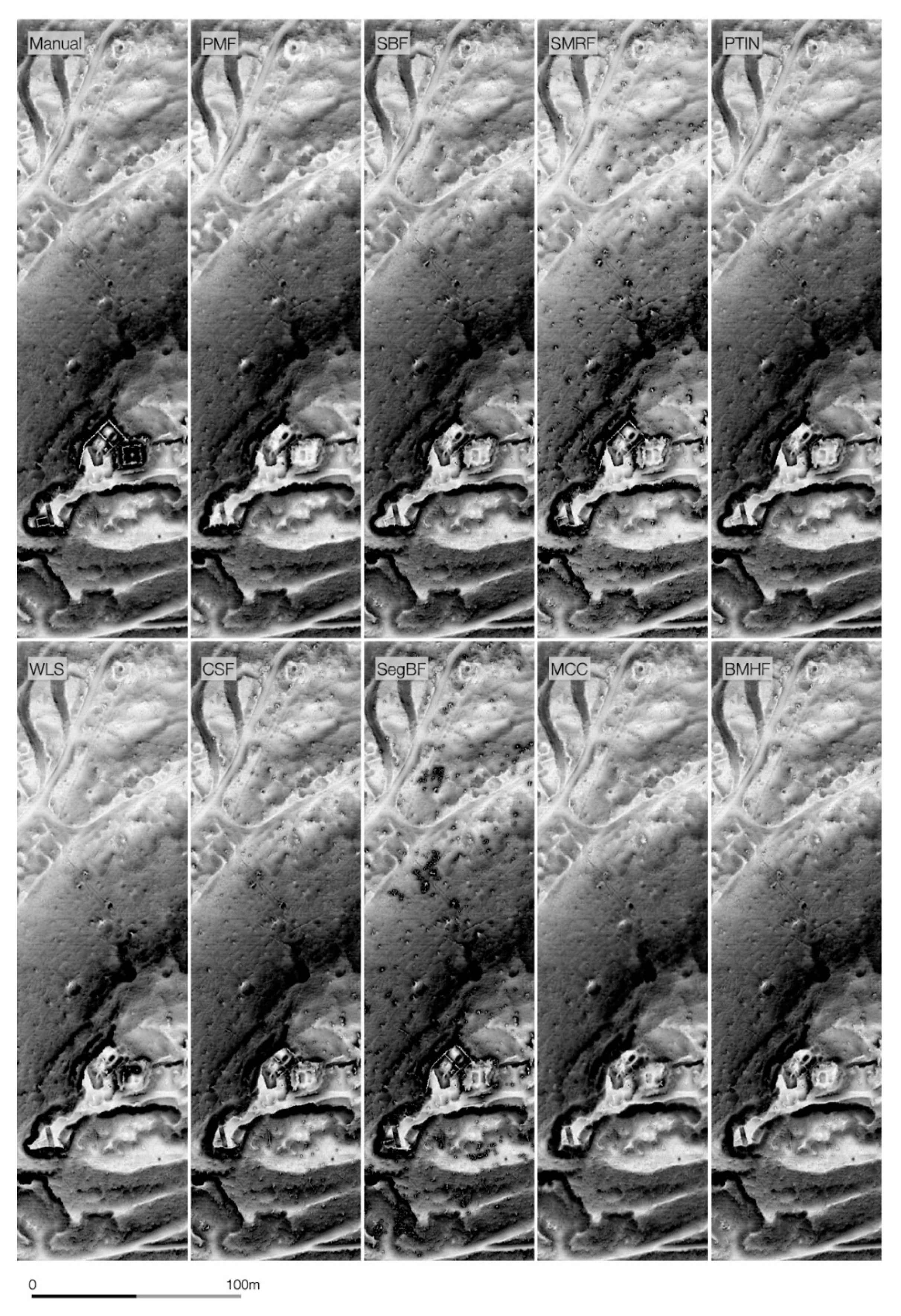
Figure 2.
Test site AT, visualizations of 0.25 m DFM’s obtained with each of the tested filters; ordinary kriging interpolation (default settings; created with Goldensoftware’s Surfer 17.1) and Sky-view factor visualization (default settings, 8-bit; created with ZRC SAZU’s RVT 2.2.1) were used.
Figure 2.
Test site AT, visualizations of 0.25 m DFM’s obtained with each of the tested filters; ordinary kriging interpolation (default settings; created with Goldensoftware’s Surfer 17.1) and Sky-view factor visualization (default settings, 8-bit; created with ZRC SAZU’s RVT 2.2.1) were used.

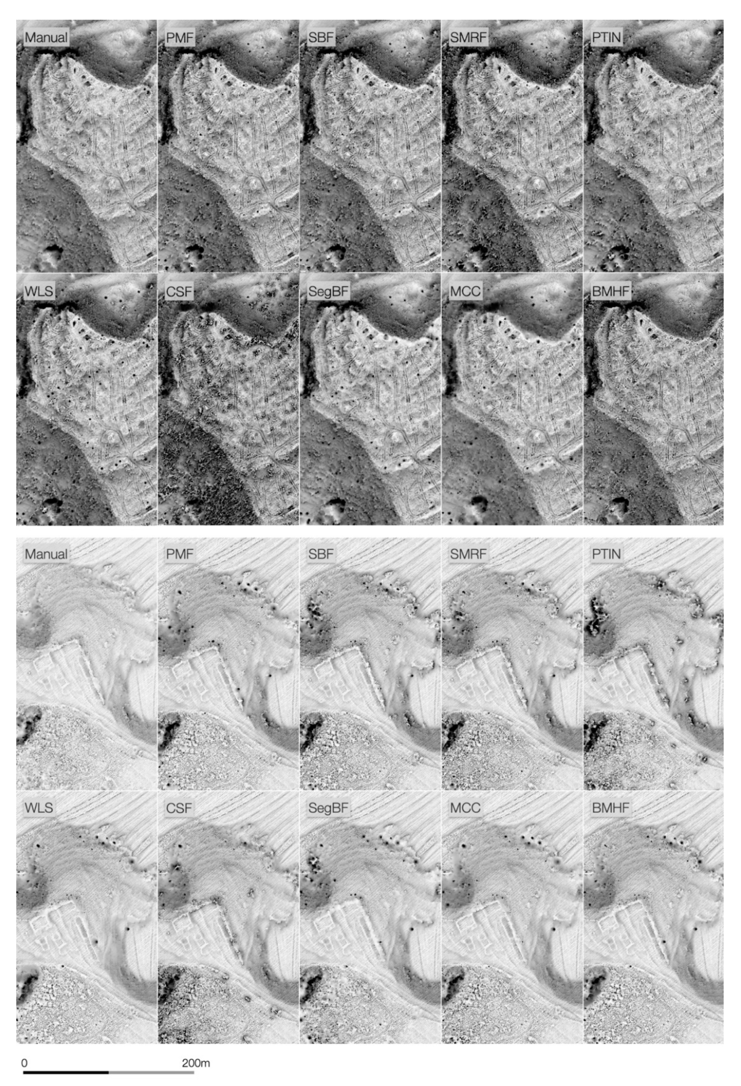
Figure 3.
Test sites SI1 and SI2, visualizations of 0.5 m DFM’s obtained by each filter; same as Figure 2.
Figure 3.
Test sites SI1 and SI2, visualizations of 0.5 m DFM’s obtained by each filter; same as Figure 2.

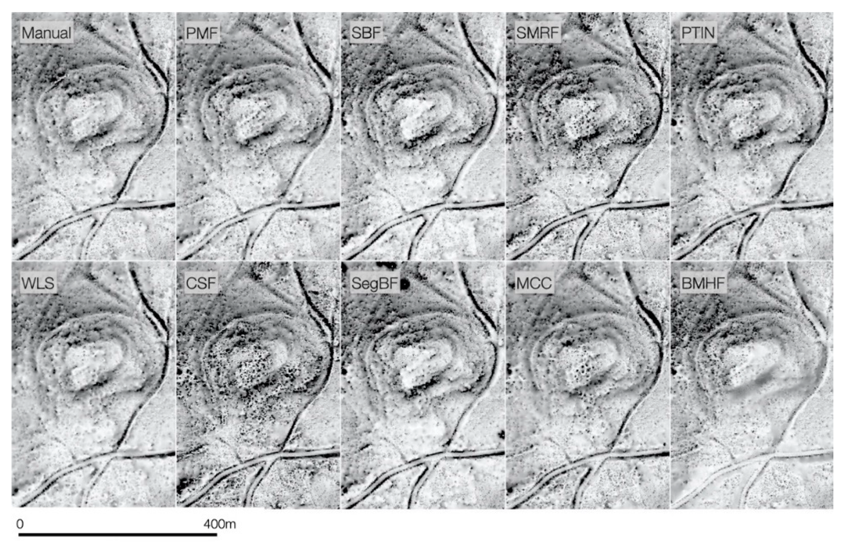
Figure 4.
Test sites SI1 and SI2, visualizations of 1m DFM’s obtained by each filter; same as Figure 2.
Figure 4.
Test sites SI1 and SI2, visualizations of 1m DFM’s obtained by each filter; same as Figure 2.

Figure 5.
Results of qualitative assessment. Individual results above, average (AVG) values bellow each category. Good ***, fair **, poor *. Archaeological features: type 1—embedded, type 2—partially embedded; type 3—standing.
Figure 5.
Results of qualitative assessment. Individual results above, average (AVG) values bellow each category. Good ***, fair **, poor *. Archaeological features: type 1—embedded, type 2—partially embedded; type 3—standing.

Figure 6.
Results of quantitative assessment.

Table 1.
Metadata on test sites.
| AT | SI1 | SI2 | ES | |
|---|---|---|---|---|
| Pnt/m2 | 18.79 | 12.28 | 12.43 | 1.83 |
| File format | XYZ | LAS/LAZ | LAS/LAZ | LAZ |
| ISPR classes | / | 0–7 | 0–7 | 0–7, 10, 12 |
| Year of acquisition | 2009 | 2014 | 2014 | 2015 |
Table 2.
Evaluated filters and software used in the study (for more details see Appendix A).
Table 2.
Evaluated filters and software used in the study (for more details see Appendix A).
| Filter | Acronym | Software | Software Type |
|---|---|---|---|
| progressive morphological f. | PMF | lidR 2.2.4 | free |
| slope-based f. | SBF | Whitebox tools | free |
| simple morphological f. | SMRF | PDAL 2.1.x | free |
| progressive triangulated irregular network | PTIN | lasground_new | commercial |
| weighted linear least-squares interpolation | WLS | Fusion 3.80 | free |
| cloth simulation f. | CSF | CloudCompare 2.10.2 | free |
| segmentation based f. | SegBF | Whitebox tools | free |
| multiscale curvature classification | MCC | MCC-LIDAR 2.2 | free |
| Blue Marble Geographic’s hybrid f. | BMHF | Global Mapper 21.x | commercial |
© 2020 by the authors. Licensee MDPI, Basel, Switzerland. This article is an open access article distributed under the terms and conditions of the Creative Commons Attribution (CC BY) license (http://creativecommons.org/licenses/by/4.0/).
Share and Cite
MDPI and ACS Style
Štular, B.; Lozić, E. Comparison of Filters for Archaeology-Specific Ground Extraction from Airborne LiDAR Point Clouds. Remote Sens. 2020, 12, 3025. https://0-doi-org.brum.beds.ac.uk/10.3390/rs12183025
AMA Style
Štular B, Lozić E. Comparison of Filters for Archaeology-Specific Ground Extraction from Airborne LiDAR Point Clouds. Remote Sensing. 2020; 12(18):3025. https://0-doi-org.brum.beds.ac.uk/10.3390/rs12183025
Chicago/Turabian StyleŠtular, Benjamin, and Edisa Lozić. 2020. "Comparison of Filters for Archaeology-Specific Ground Extraction from Airborne LiDAR Point Clouds" Remote Sensing 12, no. 18: 3025. https://0-doi-org.brum.beds.ac.uk/10.3390/rs12183025
Note that from the first issue of 2016, this journal uses article numbers instead of page numbers. See further details here.