4.1. Physiological, Biochemical, Morphological, and Remote Sensing Responses under Water Stress
Changes in leaf physiology are the result of plant-level regulation, and therefore changes in g
s, T
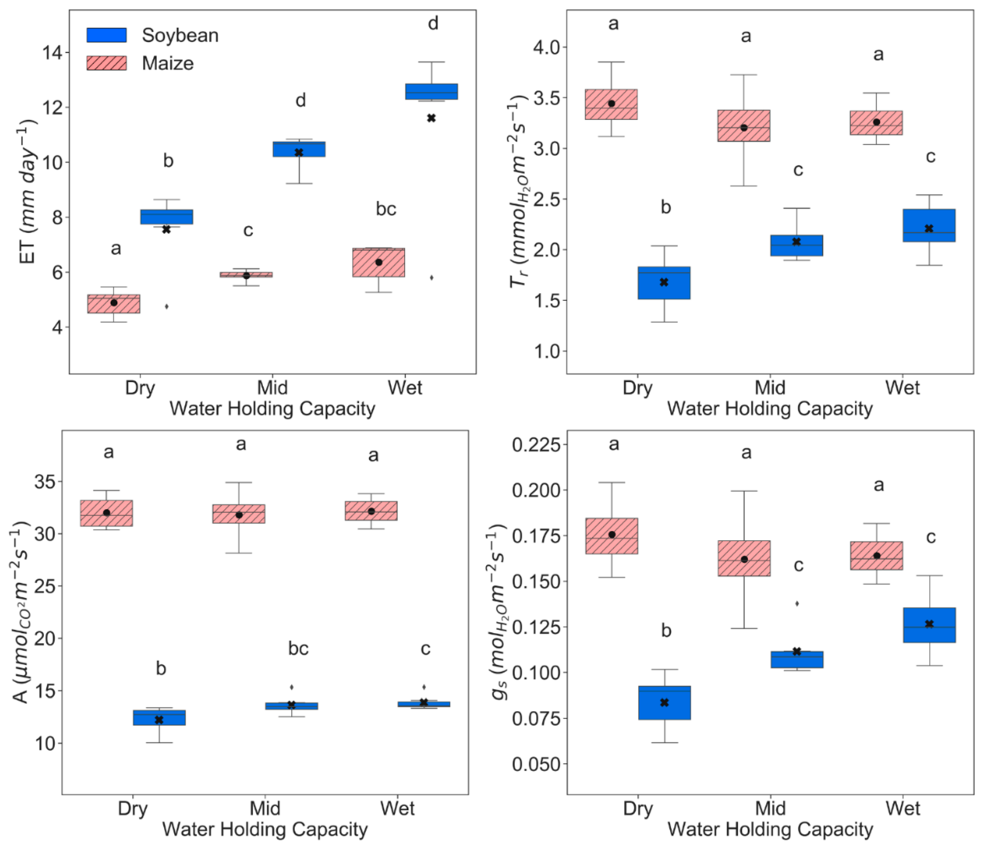
r, and A associated with soil drought have to be interpreted by looking at transpiration responses of the overall canopy. After 4–7 DoM, leaves were practically covering the full soil surface, especially in soybean plants. Thus, soil evaporation could be neglected, assuming canopy transpiration similar to ET. Our data showed that for a 60% soil water reduction, both crops experienced a significant reduction about the same order of magnitude in average canopy transpiration (around 23% for maize and 35% for soybean) (
Figure 3). However, maize and soybean plants presented different responses in T
r and g
s at the leaf level.
For soybean, a proportional decline of leaf g
s (≈34%) and leaf T
r (≈24%) was observed after the reduction of 35% ET (
Figure 3). This suggests that the strategy of soybean plants to cope with drought is through tight stomatal control, also shown by the significant rise of leaf vapor pressure deficit (VPD
leaf ≈ 13%) (
Figure S1) and T
L,Rad (≈3%) (
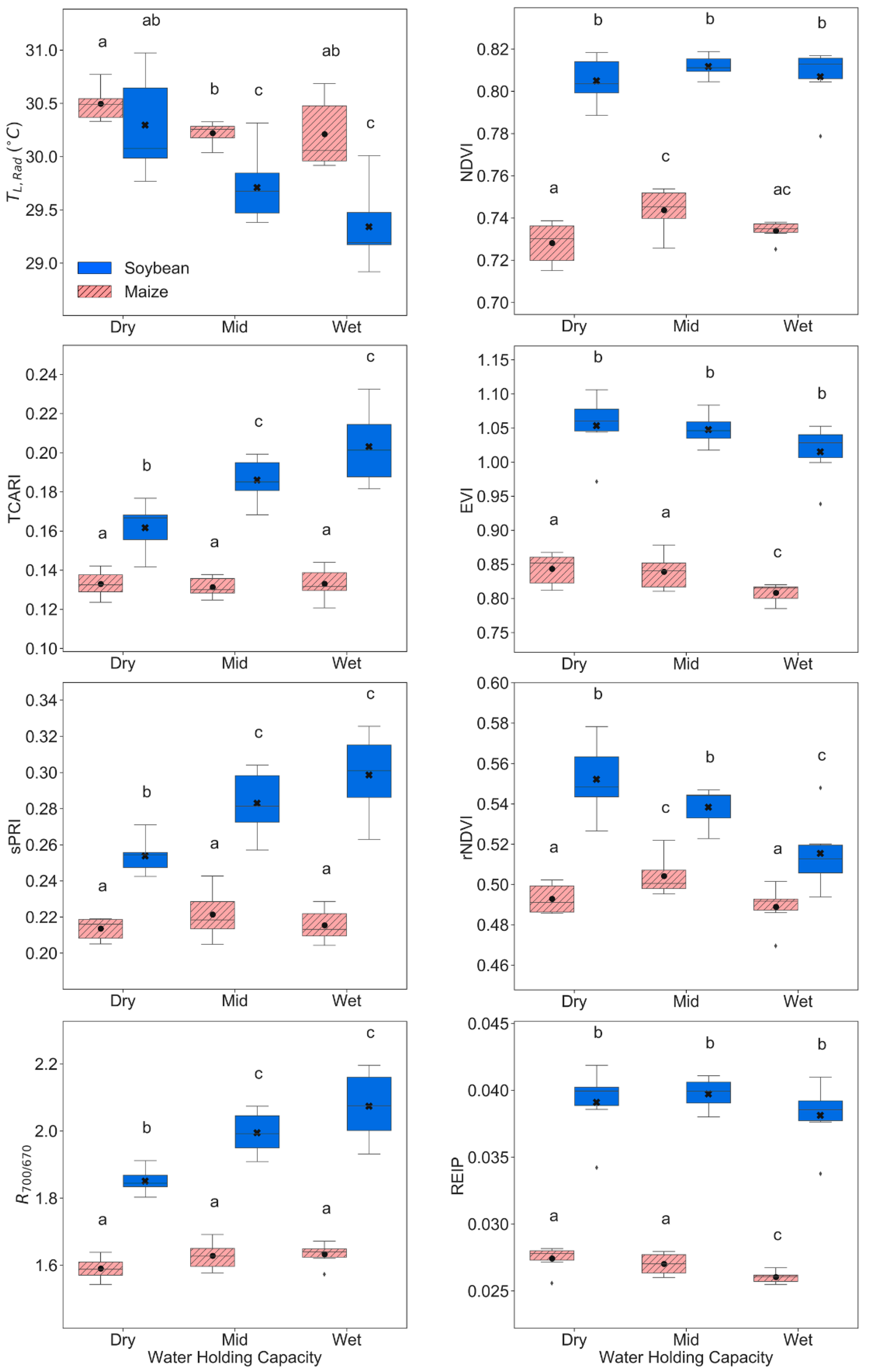
Figure 3). From this study, we found that T
L,Rad is a key remote sensing index to track drought responses in soybean plants, as it captures the warming effect from less cooling from lower T
r and g
s (
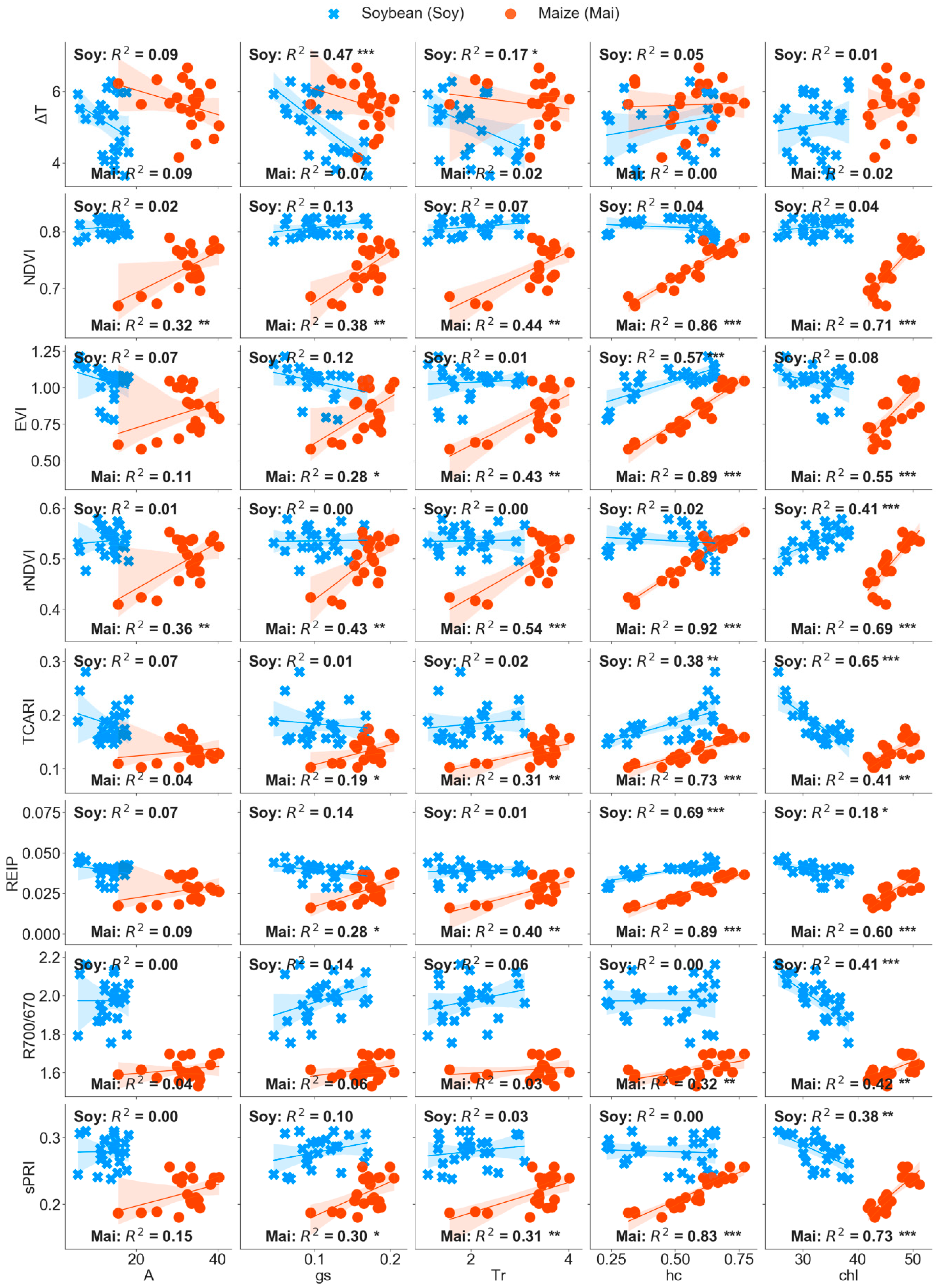
Figure 3). Furthermore, ΔT was the only index significantly correlated with soybean g
s and T
r (
Figure 6). Similar response in g
s of soybean plants has been also shown by others [
17,
19,
86]. Thigh stomatal control could be associated to soybean plants not acclimating well to soil water stress due to lack of adjustment in leaf hydraulic conductance [
87]. Thus, to avoid hydraulic failure, it tends to close stomata. As in soybean plants, most of the reduction in ET can be linked to reductions in leaf T
r, water stress impacts on growth (i.e., LAI decreases) did not seem to play a big role (
Table 3). The main support for this argument relies on LAI measurements at the end of the season with not significant differences between wet and dry soil water levels (
Table 3 and
Figure S5). In addition, remote sensing indices traditionally associated with LAI such as NDVI [
42,
53,
88], OSAVI [
37,
39,
85], and REIP [
75,
88], were not significantly affected by changes in soil water (
Table 4,
Figure 5 and
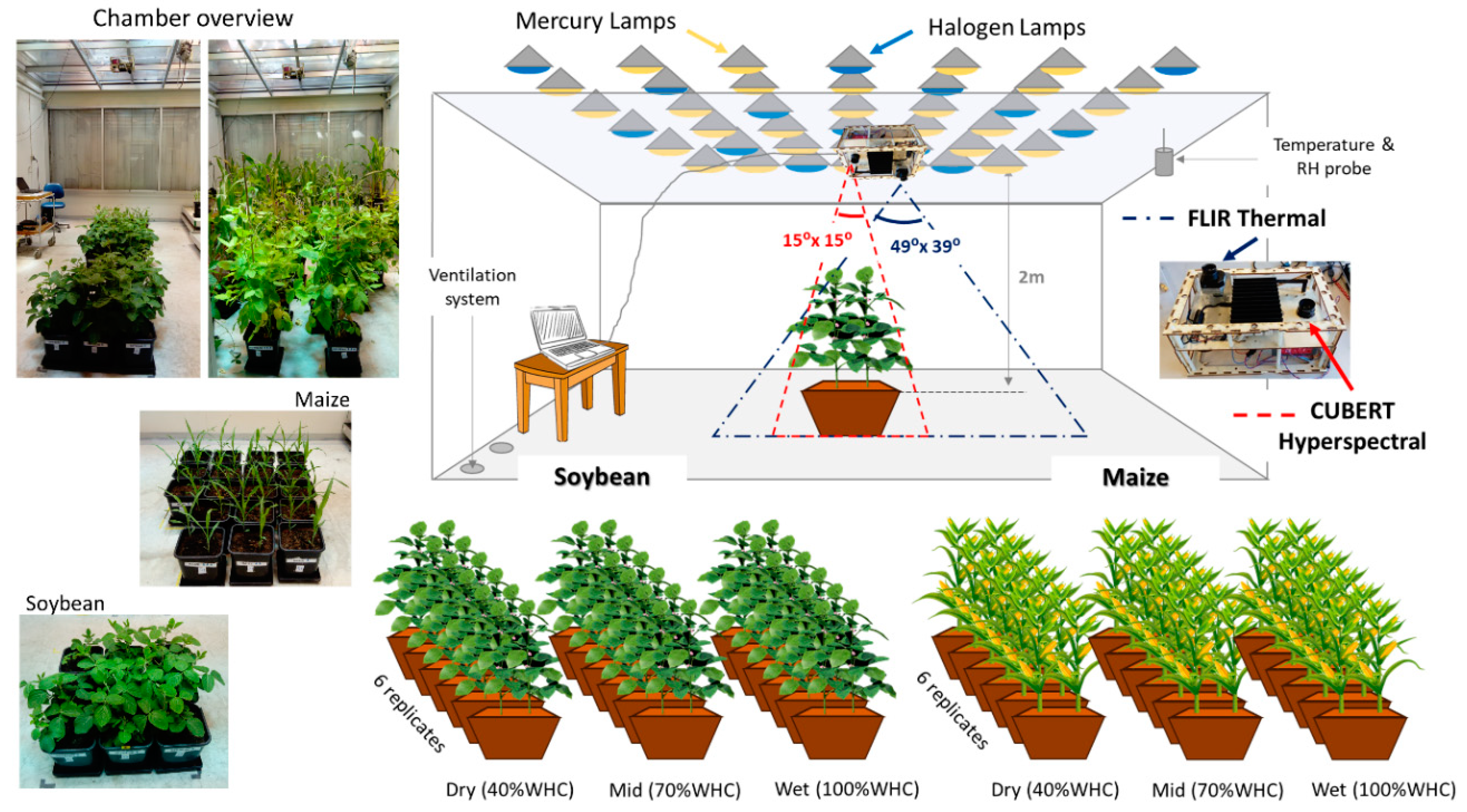
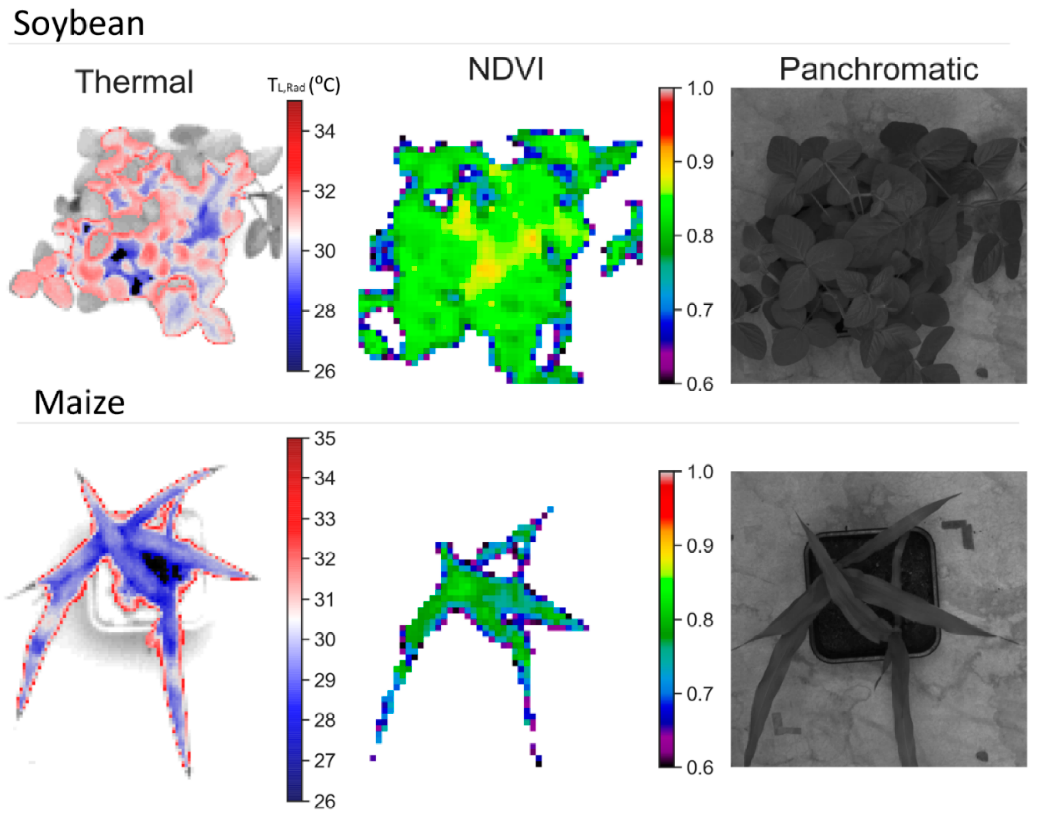
Figure S1). It is possible that, as VIs were calculated only from vegetation pixels (
Figure 2), their ability to detect decrease in LAI might be reduced. However, it can be seen that h
c, a proxy for cell enlargement and associated to growth [
7,
17], did not suffer significant changes due to drought (
Table 3). Because VIs were obtained from average pixels of top vegetation cover from a high resolution camera (10.5 mm/px), we assumed that most of the detected reflectance by the sensor was coming from top of canopy leaves and it is not considered as a composite plant-canopy reflectance. However, some of the pixels might incorporate reflectance of several overlapping leaves (
Figure 2) and leaf scattering effects might be observed on the NIR part of the spectrum [
32], which can be also related with changes in leaf angle due to drought effects [
10,
32,
89]. By removing soil background pixels (
Figure 2), we eliminated most of the reflectivity from soil, supported by similar behavior between NDVI and OSAVI, which minimizes soil effects [
70], with significant differences for soybean but not for maize (
Table 3). Thus, we could infer that soil brightness effects were low. Nevertheless, for further improvements on reflectance measurements, ‘bare soil’ reflectance for each soil water level can provide useful information to reduce soil brightness effects [
90].
In maize, all the leaf physiological variables (g
s, T
r, and A) (
Figure 3) as well as VPD
leaf and intercellular CO
2 concentration (C
i) (
Figure S1) were very similar among WHC groups. Nonetheless, such differences in T
r and A were enough to result in a significantly lower water use efficiency (WUE ≈ 10%) with 60% reduced soil water availability (
Figure S1). Therefore, the detected 23% drop of ET under soil water stress (
Figure 3) must be mostly driven by a reduction in LAI, as morphological adjustments are an effective mechanism to cope with water stress in maize plants [
8]. Our results support this hypothesis, where measurements of LAI performed at the end of the experiment were significantly lower with water stress for maize but not for soybean (
Table 3 and
Figure S5). Moreover, structural related VIs such as NDVI, rNDVI, OSAVI, EVI, and REIP showed significant effects between soil water levels (
Table 4) and significantly positive relations between these VIs with g
s and T
r (
Figure 6 and
Figure S4). In recent studies, structural VIs have also successfully been used to predicted water stress proxies (e.g., g
s, leaf water content, and leaf water potential) in maize plants [
91,
92]. In our study, the effect of growth through these VIs is shown by the high sensitivity of phenology (DoM), lack of significance with soil drought (WHC) (
Table 4), and the strong positive correlations with h
c (R
2 > 0.86) (
Figure 6 and
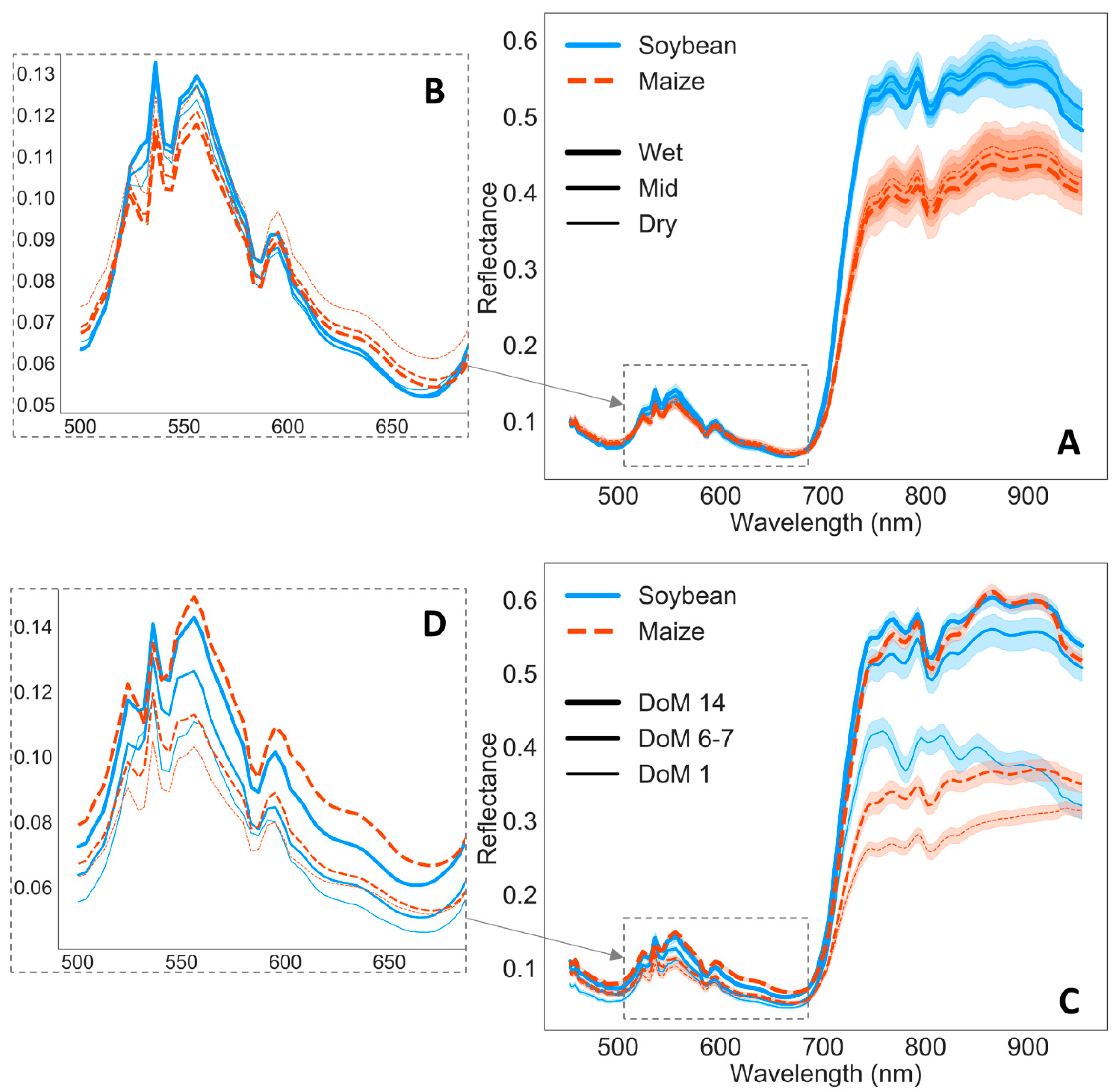
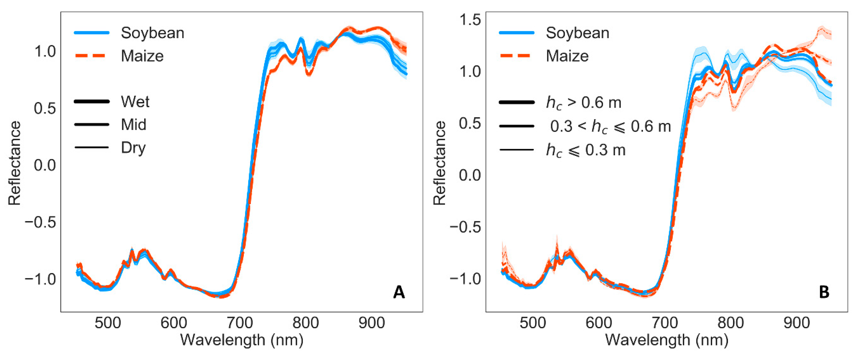
Figure S4). In addition, maize reflectance presented higher reflectance over time than soybean (
Figure 4C,D), which indeed could imply more variability due to growth, as changes in LAI can be detected in the NIR region close to the red-edge [
56,
75]. In contrast to soybean, maize T
L,Rad was not sensitive to drought (
Table 4) and ΔT did not vary with phenology. In addition, ΔT was the only remote sensing variable not related to any maize parameter (g
s, T
r, A, h
c, and chl) (
Figure 6). Unlike our results, others studies of greenhouse maize plants have been successful in detecting drought through thermal imaging, likely due to higher air temperature (27–28 °C) increasing soil water stress [
50,
93].
Despite of such a large mean reduction in soybean g
s from wet (100%) to dry (40%) WHC, soybean plants significantly increased about 15% their WUE (
Figure S1) as they only experienced a small decrease in A (≈12%) relative to the reduction in transpiration at canopy and leaf levels (
Figure 2). These could be explained by a 16% mean increase in top leaves chl concentration, measured with SPAD (
Figure S1). Zhang et al. (2016) [
19] also found increased chlorophyll content as well as decreased g
s, T
r, and A in greenhouse soybean plants with soil water reductions of about 40%. However, they reported declines in WUE of about 45%. Wijewardana et al. (2019) [
17] have interpreted WUE increases as an adaptive mechanism to drought due to transpiration decline under soil moisture stress in soybean plants. However, in their experiment, they observed a 24% decrease on chlorophyll content of soybean plants with 38% increase in carotenoids. Explanations to differences among studies might be associated to experimental design. For instance, plants in Wijewardana et al. (2019) [
17] were exposed to higher radiation and temperatures (29 °C) than in our experiment, with a longer cycle, which would increase soil water stress. Cultivar types also present different morphological and physiological adjustments to drought [
7,
86].
Moreover, VIs used to detect changes in chlorophyll concentration (TCARI, TCARI/OSAVI, and R
700/670) can track responses to soil drought across different dates, especially for R
700/670 (
Table 4,
Figure 6 and
Figure S4). Unlike soybean, maize leaf chl did not change across soil water levels (
Table 3), reflected also in the lack of significance in TCARI and TCARI/OSAVI indices. However, this was not the case for R
700/670 (
p-value < 0.01) (
Table 4), likely because this VI does not minimize LAI variations as TCARI and TCARI/OSAVI [
39]. Differences on chl response between crops can be related to decreased soybean reflectance in the VIS with soil drought (up to around 640 nm), whereas maize reflectance increased (
Figure 4A,B). Similarly, Feng et al. (2013) [
94] found greater maize reflectance under soil water stress in this region. VIs linked to photosynthetic efficiency like PRI are often used to detect soil moisture changes [
37,
41,
43,
45,
76]. However, PRI is also quite sensitive to structural changes, pigment levels, soil background, illumination effects, and viewing angles [
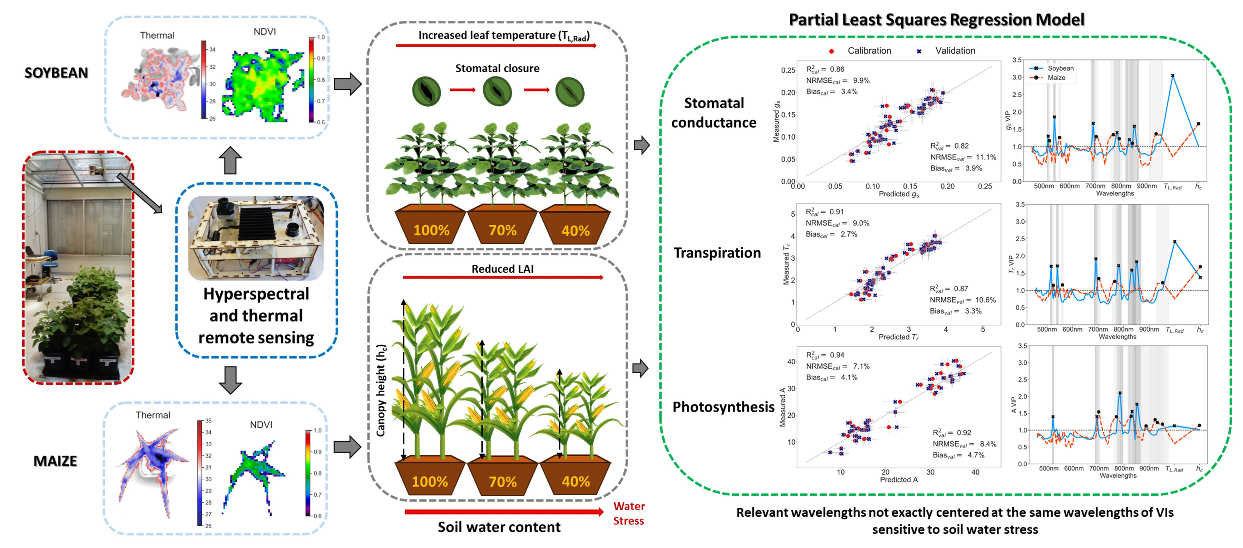
42,
43]. As the experiment was conducted in a growth chamber with high-pressure mercury and halogen lamps (peak at 538 nm), some of the PRI results might not be like in field conditions (
Figure 3). However, variations of PRI calculated with other bands as sPRI (510 nm and 560 nm) and PRI
570–515 were significantly reduced presenting less photosynthetic activity with drought (
Table 4), especially for soybean plants (C
3) as they are less efficient than C
4 species (maize) [
21,
22]. Note that soybean sPRI as well as R
700/670 were not influenced by changes across time (
Table 4), making them attractive to detect drought in soybean plants, likely subtracting growing effects. Unlike soybean, not a single maize VI was only significant across water groups (
Table 4).
One area of interest is the possibility to use remote sensing to detect isohydric and anisohydric behavior, which is concept related to leaf water potential (Ψ
L) [
95]. Leaf water content can be retrieved from optical (between 800 nm and 2500 nm) and microwave radiation [
10]. In our experiment, because our hyperspectral camera only covers the VNIR region (400–900 nm), we did not measure Ψ
L. However, if reductions in g
s are linked to reductions in Ψ
L as shown by Wijewardana et al. (2019) [
17], it could be inferred that soybean plants behaved more as isohydric crop compared to our type of maize plants. This could also be associated with the type of photosynthetic pathway as C
3 species such as soybean tend to exhibit more considerable reductions in g
s than their C
4 relatives under drought [
23]. Nevertheless, according to Costa et al. (2013) [
48], g
s is better indicator of soil water stress in isohydric plants, enabling thermal imaging to better detect drought, as we observed in our results (
Figure 6). In addition, Konings et al. (2017) [
25] also identified a maize cultivar as anisohydric. Still, the concept of iso/anisohydric appears more complex than can be represented as a binary factor, and could instead occur as a response to environmental thresholds or occur along a continuum [
95,
96]. Therefore, discrepancies in this classification are found for soybean [
48,
97] and maize crops [
16,
48,
97,
98,
99].
4.2. Synergies of Optical, Thermal, and Canopy Height Observations for PLS-R Modeling
In response to drought severity and duration, crops undertake different adjustments in plant physiology, morphology, and biochemistry. Some of those changes are noticeable from the drought onset (fast changes), while others are noticeable only after some time, also referred as slow changes [
10]. For example, stomatal closure occurs practically instantaneous under water stress, while effects on chlorophyll content and structure tend to be visible after longer periods of time [
10,
11,
13]. Our study showed that for soybean plants T
L,Rad was a faster indicator of physiological adjustments than VIS indices such as NDVI and PRI (
Figure 6 and
Figure S4) as shown also by [
45,
100,
101]). Nonetheless, improved detection of water stress can be achieved by combining thermal and optical imaging [
37,
46,
47,
102], as the energy balance is affected by drought. The temperature is the result of the balancing of several processes, including transpiration cooling and absorption of radiation. For example, maize plants were warmer than soybean plants (
Figure 5), despite presenting higher T
r for any soil moisture condition (
Figure 3).
Figure 4A shows how maize wet plants reflected less energy than wet soybean in the VNIR wavelengths, indicating more energy absorption, translated in significantly higher thermal emission. From the point of view of plant physiology, although h
c is a parameter at the canopy level, it integrates leaf level processes in response to stress: e.g., cell enlargement has been shown very sensitive to water stress [
11,
13], and h
c reduction could be associated with decrease on cell enlargement [
7,
17]. For this reason, h
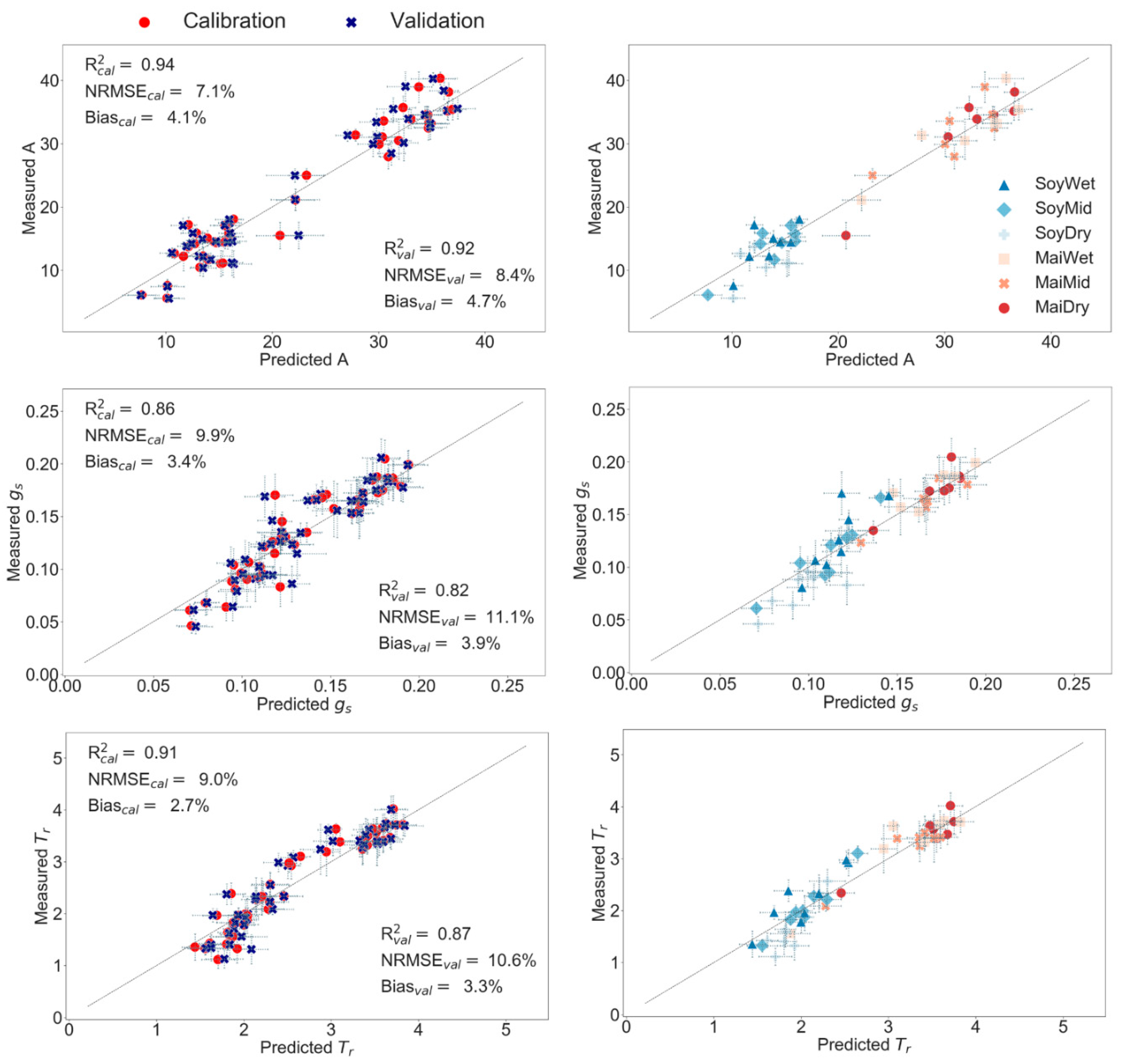
c was used as predictor for water stress. In addition, h
c is a growth indicator easily obtained from remote sensing [
52], that provided valuable information to model g
s, T
r, and A (
Figure 9).
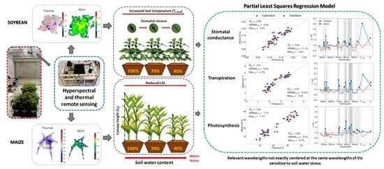
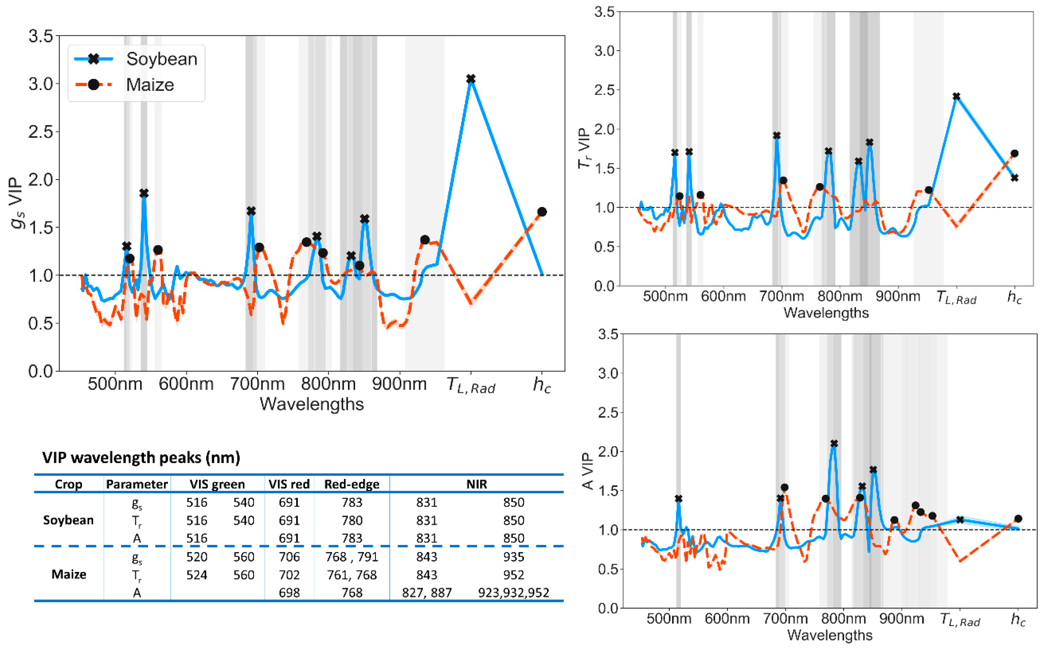
PLS-R is not only a tool to model crop physiology parameters, but the VIP scores can inform of the more relevant wavelengths and variables responding to soil drought. In fact, the highest VIP scores for g
s and T
r correspond to T
L,Rad in soybean and h
c in maize (
Figure 9), reflecting the dominant effects of soil drought: stomatal closure on soybean and plant growth on maize plants. Moreover, model improvements were appreciated in soybean g
s model when including T
L,Rad predictor, and in maize T
r model when adding h
c (
Table 5). A curious fact when looking at hyperspectral band contribution was that soybean crops shared importance on similar wavelengths among A, g
s, and T
r, whereas maize response varied between traits with low VIP signal (
Figure 8). From this, we can speculate that soybean processes are more interdependent than maize mechanisms.
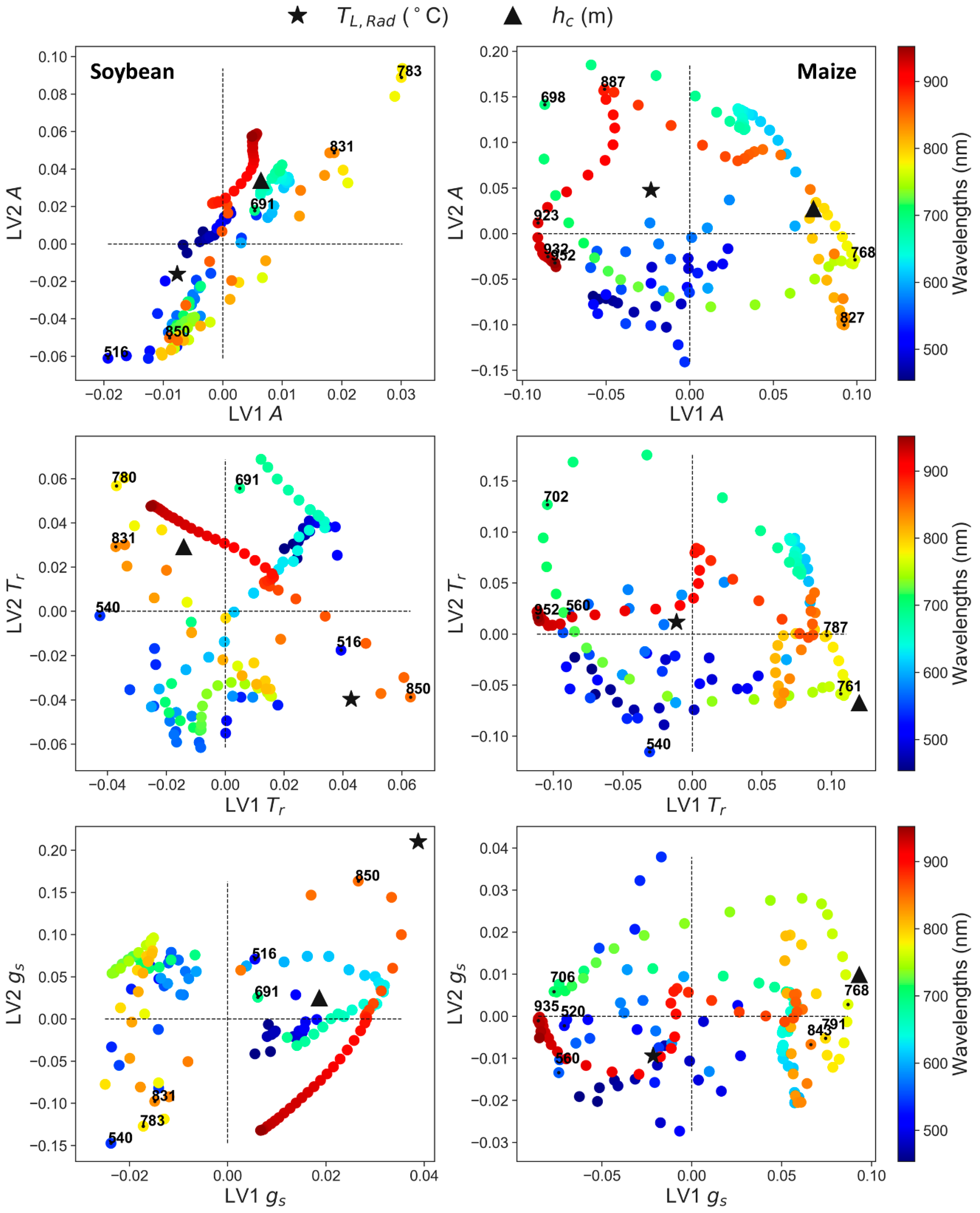
Because part of the information obtained from the new variables (T
L,Rad and h
c) could be implicit in some of the 138 bands of the hyperspectral sensor, we looked into the relation between LV1 and LV2 for all predictors (
Figure 10). Overall, we found that most of the bands showing high VIP scores (
Figure 9) were correlated with T
L,Rad and h
c (
Figure 10). These correlations could explain why model performance did not improve remarkably by adding the two new predictors (
Table 5). For soybean g
s, T
r, and A peaks with VIP scores above one were found in regions that correspond to absorption of chlorophyll b (516 nm), chlorophyll a (691 nm), red edge (780–783 nm), and the NIR plateau (831 and 850 nm) (
Figure 9). Most of these bands clearly overlap the ones used in the VIs studied (
Table 2), but they are not exactly centered at the same wavelength, highlighting the importance of using hyperspectral remote sensing with contiguous narrowband. Further research would be needed to confirm this finding across different illumination sources and conditions.
Regions around 515 nm and 700 nm have been reported to be very suitable to estimate A and indirectly g
s due to their ability to detect chlorophyll changes [
42,
75]. Similar to our result for soybean, Matthes et al. (2015) [
55] found maximum VIP scores between 670 and 680 nm when using PLS-R to predict GPP and NEE in pasture and rise sites under Mediterranean climate. In addition, a recent study concluded, based on PLS-R VIP analysis, that most important bands to predict wheat g
s, T
r, and A from hyperspectral data were mainly placed in the VIS and red-edge regions [
57]. Wavelengths around 780 nm presented one of the highest VIP values in soybean g
s, T
r, and A, in agreement with mARI being sensitive to T
r. Note that narrow wavebands (831 and 850 nm), often combined with water absorption bands in SWIR to obtain water and moisture indices [
42], were not used in VI calculations. In
Figure 9, soybean T
r and g
s VIP showed also a spike centered at the green band 540 nm, which might be partly due to artifacts caused by artificial illumination sources (
Figure 4). Nonetheless, Rapaport et al. (2015) [
15] also found that this band was one of the bands contributing the most to estimate leaf water potential to detect water stress under solar irradiance conditions.
In relation to artifacts caused by the lamps (
Figure 4), to some extent, they should be removed when calculating reflectance by the normalization with incoming irradiance and the normalization prior to PLSR processing. Even though it is possible that some of these artifacts could be related to temporal changes in the lamp’s irradiance caused by voltage oscillations, other authors have found similar effects in reflectance due to lamps irradiance spikes. Schuerger & Richards (2006) [
103] investigated reflectance of healthy and water stressed pepper plants under seven artificial illumination sources and they found that high pressure sodium and metal halide lamps, with irradiance spikes similar to those in our high pressure mercury and halogen lamps, introduced spikes in the reflectance spectra. Thus, peaks in the spectral irradiance distribution of the lamps, compared to the solar irradiance, may modify mostly plants reflection while the absorbed light might not be affected in the same proportion, and, therefore, plants release the extra light. Nevertheless, these small reflectance artifacts do not seem to show an inconvenient to effectively detect plant changes in reflectance due to water stress under these type of lamps [
103].
Unlike soybean, the contribution of wavelengths to maize g
s, T
r, and A PLS-R modeling was more spread over the whole spectra with lower VIP scores (
Figure 9). Nonetheless, there were a few common regions with spikes at two red-edge wavelengths (around 700 and 760–780 nm). Note that bands around 770 nm were near to h
c, explaining similar trend. This was not the case for 700 nm presenting negative loading in the first LV (
Figure 10). These bands are closely related to the rNDVI (705 and 750 nm), which relate to structural changes to detect drought [
76]. Bands at 705 nm and 700–740 nm relate to water stress while 760 nm accounts for water absorption [
42]. In line with this and using PLS-R, strong relations were found between red-edge bands and V
cmax (correlated to A) in nine agricultural crops [
58]. In
Figure 9, green bands (around 520 and 560 nm) for predicting maize g
s and T
r showed important contribution, but not same information as h
c (
Figure 10). These bands were not used in VI calculations, despite being close to PRI and its variants (
Table 2). Thus, they could be potential wavelengths to predict maize g
s and T
r under water stress. NIR band (843 nm) was also important (
Figure 9). h
c has been previously related with near infrared bands [
42], associated with LAI and leaf scattering [
32]. Maize A VIP was substantially higher at around 890 and 920–950 nm, while T
r VIP was prominent at 952 nm and g
s VIP at 935 nm (
Figure 9). In the NIR spectral bands, water absorption features are identified around 900 and 970 nm (water index) [
104]. Although our hyperspectral sensor detected changes related to water absorption between 870 nm and 960 nm, these wavelengths were more noisy than VIS bands with wider full width at half maximum (
Figure 9). Thus, the models might not detect high signals in water bands. According to Taylor et al. (2011) [
23], in C
4 species, drought effects in A and T
r might be more visible in the whole plant rather in specific leaf compared with C
3 plants.
Finally, it is worth mentioning that this study was conducted during a short vegetative period of two crops under specific controlled environmental conditions, presenting certain limitations. Thus, to assure the reproducibility of these results, further research will be required in more species, repeating and testing the method in a larger dataset as recommended by Matthes et al. (2015) [
55]. In addition, a step further will be to apply this study under external ambient conditions as similarly done by Rapaport et al. (2015) [
15].

 ,
, 


