Article

Evaluation of Remote Sensing-Based Irrigation Water Accounting at River Basin District Management Scale

1
Remote Sensing & GIS Group, Institute for Regional Development, University of Castilla-La Mancha, Campus Universitario s/n, 02071 Albacete, Spain
2
Deputy Directorate for Water Planning, DG Water—Ministry for the Ecological Transition and the Demographic Challenge (MITERD), 28071 Madrid, Spain
3
Deputy General Directorate of Irrigation, Natural Roads and Rural Infrastructures, Spanish Ministry of Agriculture, Food and Fisheries, 28005 Madrid, Spain
*
Author to whom correspondence should be addressed.
Remote Sens. 2020, 12(19), 3187; https://0-doi-org.brum.beds.ac.uk/10.3390/rs12193187
Submission received: 3 August 2020 / Revised: 21 September 2020 / Accepted: 25 September 2020 / Published: 29 September 2020

Abstract

:
The Water Framework Directive in Europe requires extending metering and water abstraction controls to accurately satisfy the necessary water resource requirements. However, in situ measurement instruments are inappropriate for large irrigation surface areas, considering the high investment and maintenance service costs. In this study, Remote Sensing-based Irrigation Water Accounting (RS-IWA) (previously evaluated for commercial plots, water user associations, and groundwater water management scales) was applied to over 11 Spanish river basin districts during the period of 2014–2018. Using the FAO56 methodology and incorporating remote sensing basal crop coefficient time series to simulate the Remote Sensing-based Soil Water Balance (RS-SWB), we were able to provide spatially and temporally distributed net irrigation requirements. The results were evaluated against the irrigation water demands estimated by the Hydrological Planning Offices and published in the River Basin Management Plans applying the same spatial (Agricultural Demand Units and Exploitation Systems) and temporal (annual and monthly) water management scales used by these public water managers, ultimately returning ranges of agreement (r2 and dr) (Willmott refined index) of 0.79 and 0.99, respectively. Thus, this paper presents an operational tool for providing updated spatio-temporal maps of RS-IWA over large and diverse irrigation surface areas, which is ready to serve as a complementary irrigation water monitoring and management tool.

Graphical Abstract

1. Introduction

AQUASTAT, the global information system on water resources, quantifies and differentiates human water abstractions based on three use categories: municipal (11%), industrial (19%), and agricultural (70%) [1]. At the continental level, Africa and Asia have an agricultural proportion of 80%, while the water used in Europe for agriculture makes up 21%. However, the same balance changes drastically over Mediterranean regions, where 80% of freshwater is abstracted for agricultural purposes [2].
Considering “the need for action to protect Community waters in qualitative as well as in quantitative terms” and the fact that “Waters in the Community are under increasing pressure from the continuous growth in demand for sufficient quantities of good quality water for all purposes”, the European Commission created DIRECTIVE 2000/60/EC [3], commonly known as the Water Framework Directive, in which a common framework for similar actions related to water is proposed. Unlike the more common use of administrative or political boundaries, the Water Framework Directive selects the River Basin District (RBD) as the common geographical and hydrological unit of interest, for which the River Basin Management Plan (RBMP) is needed to provide a detailed account of how the objectives set for the RBD will be reached within the timescale required [4]. With a lifecycle of six years, the RBMPs are presently in their second cycle (the period of 2015–2021).
Recently, the fifth European Commission report about the implementation of the Water Framework Directive by the RBMPs notified southern Europe that irrigation water is the principal pressure agent in water abstraction and suggested that relevant actions are required to extend the relevant metering and water abstraction controls [5]. By contrast, public water managers in charge of RBDs have already expressed dissatisfaction about using a water metering network solely based on volumetric meters, based on the high investment and maintenance costs implicated [6,7]. In the same vein, the Spanish National Centre of Irrigation Technology stated that each volumetric meter must be correctly installed to produce reliable results in successive years; later, correct maintenance must be implemented to prevent water residues from producing incorrect water records [6,7]. Therefore, there is a conflict between the legal framework, which expresses the necessity to establish and extend irrigation water accounting over large and diverse areas, and the inappropriate long-term use of in situ measurement instruments.
In this context, an important remote sensing characteristic is a large capacity for data acquisition over large areas. Presently, two of the satellites most commonly used for vegetation cover monitoring are Landsat 8 and Sentinel-2 (twins A and B), which cover 185 and 290 km swaths, respectively, as well as having spatial resolutions of 30–100 m (Landsat 8) and 10–60 m (Sentinel-2). Satellite images provide real-time information about the vegetation cover state, which, together with the temporal resolution (15 days in Landsat 8 and up to 5 days in Sentinel-2), allows the monitoring of vegetation evolution through remote sensing time series. Moreover, both satellites are supported by strong programmes that freely provide the satellite images to the public to return the related environmental and economic benefits to society [8,9].
In parallel, the FAO56 Irrigation and Drainage Paper number 56 Crop Evapotranspiration (ETc) provides guidelines for determining Crop Water Requirements [10] through globally homogenised methodologies combining evaporative atmospheric demands accurately calculated over a reference crop surface (also called reference evapotranspiration (ETo)) and a dimensionless crop coefficient (Kc) that expresses the evapotranspiration difference between the crop surface and the reference surface. Moreover, ETc estimation has two approaches: a single crop coefficient or a dual crop coefficient [11]. The latter divides Kc into the evaporative component (Ke, the soil evaporation coefficient) and its transpiration component (Kcb, the basal crop coefficient). Moreover, when crops suffer water restrictions, the water stress coefficient (Ks) is incorporated into the method to estimate the adjusted crop evapotranspiration (ETc adj).
The use of remote sensing techniques in the FAO56 methodology to estimate ETc follows different approaches, that Calera et al. [12] classified as: remote sensing surface energy balance [13,14,15], remote sensing-based Penman–Monteith direct approaches [16,17], and reflectance-based basal crop coefficients [18,19,20,21]. The first technique uses the vegetation surface temperature to estimate the actual ETc after accounting for the energy balance. This technique is able to monitor large areas while avoiding Kc calculations and is thus appropriate for diverse vegetation cover monitoring but inappropriate for use in large and diverse irrigation surface areas at a low temporal resolution and inappropriate spatial resolution [22]. The second approach uses the optical spectral range to obtain crop parameters (the leaf area index, albedo, and crop height) to include them into the Penman–Monteith equation and directly estimate ETc. This approach allows one to monitor large areas at adequate spatial and temporal resolutions for crop monitoring with operational applications used to monitor and determine irrigation surface areas [17]. However, several limitations are still present in ETc estimations regarding the crop-dependency relationships for the crop height or leaf area index, as well as high uncertainties in determining water stress or soil evaporation effects [12]. The third approach also uses the optical spectral range to convert reflectance values into Vegetation Indexes (VI) that are empirically related through linear relationships with Kc and Kcb [21,23]. Thus, in combination with local ETo records, this approach estimates ETc over large areas. Moreover, this approach’s spatial resolution is adequate for crop monitoring (operational applications are already being implemented) [24,25,26]. However, several limitations must be considered for ETc estimation. Because this approach is supported by agrometeorological stations that register ETo, soil evaporation is not included in the formulation, and the linear relationships may vary by crop type [22].
However, for irrigation water accounting, Pereira and Alves [27] distinguished between Crop Water Requirements and Irrigation Water Requirements. While the former is the sum of the depth of water needed over the crop cycle and provided by the environment as precipitation (P) or soil water content, to satisfy the water consumed through evapotranspiration (ETc) under optimal conditions or the adjusted crop evapotranspiration when conditions deviate from optimal levels (commonly expressed as ETc − P), the latter is the net depth of water provided by irrigation systems to satisfy crop water requirements during crop development when precipitation, soil water content, or groundwater contributions are not enough. Therefore, considering previous remote sensing approaches to ETc estimation, the sum of such variable at the end of the crop cycle corresponds to the crop water requirements; thus, it is necessary to determine the soil water balance at the root depth to derive irrigation water requirements [10,27].
One relevant case is irrigation agriculture at the national level in Spain. The last report from the Ministry for the Ecological Transition and the Demographic Challenge regarding the actual state of RBMPs [28] determined the different national sources of irrigation surface areas to be about 3.6 Mha on average, which indicates annual gross irrigation water demands of about 25,800 hm3. The superficial and groundwater origin resources are estimated to be 72% and 22%, respectively (this difference is provided by non-conventional sources [28]). The latest report on irrigation by the agricultural authorities [29] established that irrigation surfaces irrigated with drip systems comprised about 53% of the total, while sprinklers and surface irrigation systems comprised about 23% each. Finally, the same report stated that irrigated crop surfaces were distributed approximately as follows: cereal crops (25%), olive trees (22%), vineyards (10%), fruit trees (10%), citrus trees (8%), forage crops (7%), horticultural crops (7%), and industrial crops (6%).
In a legal context, the Water Framework Directive was transposed into three Spanish laws [30,31,32] that configure the normative context for the RBMPs. Later, the different Hydrological Planning Offices for each RBD estimated the irrigation water demands at different spatial and temporal irrigation water management scales. Hence, annual and monthly irrigation water demands are published in the RBMPs for different and spatial management scales according to increases in the surface area and area of influence, including the Agricultural Demand Unit (ADU), the Exploitation System (ES), and the whole RBD. The ADU is defined as agricultural surfaces with common characteristics such as geographic locations, water user associations, and irrigation technologies that also share the same sources of water. Their irrigation returns are incorporated into the same zone or sub-zone in the general system. In parallel, ESs are water bodies or groups of water bodies that share surface water and groundwater, hydraulic infrastructure installations, and water use and exploitation rules.
Bearing in mind the context described above, this paper presents research that aims to evaluate Remote Sensing-based Irrigation Water Accounting (RS-IWA) over large and diverse irrigation surface areas. This model was evaluated over 11 Spanish RBDs over the period of 2014–2018. The remote sensing data, such as the VI time series, results, thematic cartography, and methodological reports are freely available from SPIDERwebGIS® (http://maps.spiderwebgis.org/login/?custom=spider-siar).
Taking into consideration the large and diverse irrigation surface areas to be monitored, the capacity for remote sensing data acquisition over such areas, the ETc estimation approaches previously described, and the necessity to derive a soil water balance to estimate the irrigation water requirements for comparison with the irrigation water demands published in the RBMPs, this project developed a Remote Sensing-based Soil Water Balance (RS-SWB) technique that follows the FAO56 methodology under the assumed criteria of homogeneity, simplicity, replicability, and reliability to estimate the irrigation water demands over large and diverse irrigation surface areas. Hence, the Landsat 8 and Sentinel-2 satellites were selected, as they offer adequate spectral, temporal, and spatial resolutions for crop monitoring and ETc estimations. Particularly, we used the reflectance-based basal crop coefficient approach, which is linearly related with the VI, as the Kcb is later incorporated into a dual crop coefficient approach to derive the ETc adj under a soil water balance scenario, which ultimately provides spatially and temporally distributed maps of the net irrigation requirements (NIR). The RS-SWB was previously evaluated against different ground truths at different spatial and temporal scales, such as for commercial plots with volumetric meters and water user associations using irrigation water management data [33]. Evaluations using the national piezometric network after determining the groundwater withdrawals from the irrigation surface area greatly depend on these groundwater resources [34], as does using the annual irrigation water demands provided by the RBMPs at an RBD spatial scale in mainland Spain [35]. The next RS-IWA evaluation was performed using the same irrigation water management scales that the Hydrological Planning Offices take into consideration, including temporal (monthly and annual time scale) and ADU and ES spatial scales.

2. Materials and Methods
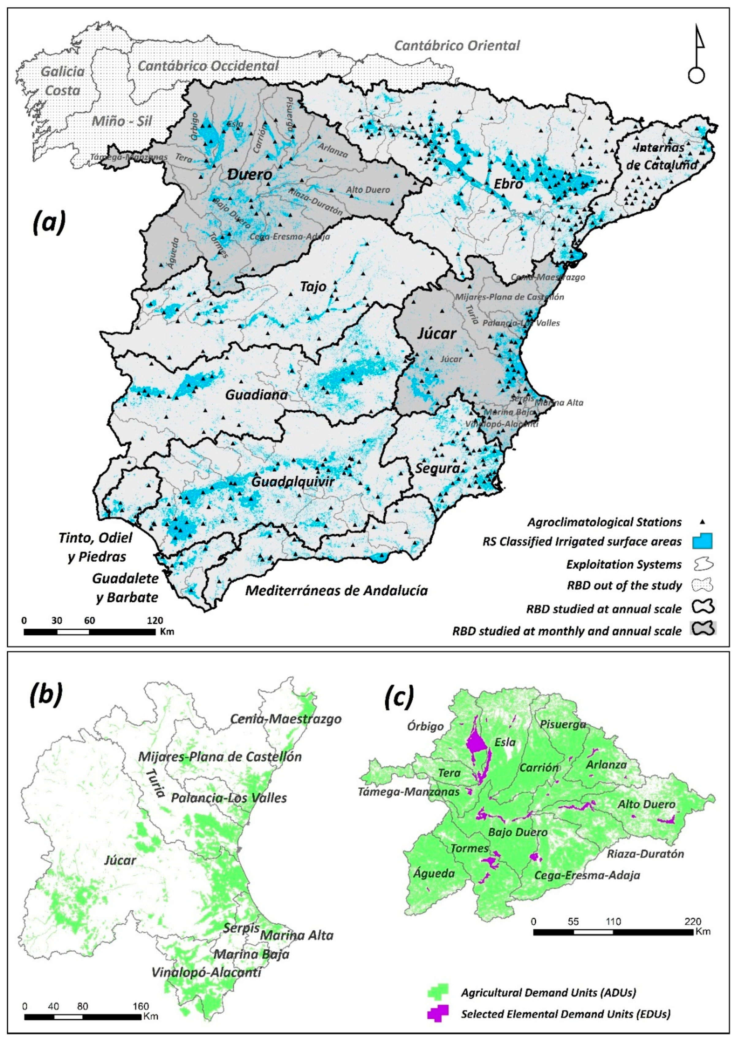
2.1. Study Area

The irrigated surface areas of 11 of the 15 RBDs in mainland Spain were monitored (Figure 1a) over the 5 study years of 2014–2018: Duero (DUE), Ebro (EBR), Internas de Cataluña (CIC), Júcar (JUC), Tajo (TAJ), Guadiana (GDN), Guadalquivir (GDQ), Segura (SEG), Mediterráneas de Andalucía (CMA), Guadalete and Barbate (GyB), and Tinto, Odiel, and Piedras (TOP). With a total surface area of about 440,000 km2 (87% of the total national surface), these 11 RBDs contain most Spanish irrigated surface areas. Hence, this extension includes great diversity and complexity in addressing diverse types of crops, irrigation systems, and agronomic management practices. The different scales of work represented in Figure 1 align with the irrigation water demands estimated by the Hydrological Planning Offices and published in the corresponding RBMPs, according to different temporal (annual and monthly) and spatial (ADU, ES, and (in the Duero RBD) Elemental Demand Unit, EDU) irrigation water management scales.
The most detailed analyses at both management scales were conducted in the Duero and Júcar RBDs and correspond to the ADU spatial management scale at a monthly and annual temporal frequency. We justify their choice over other RBDs by the diverse types of irrigated crops developed therein (herbaceous versus citrus and vineyards). In the Duero RBD, grain cereals stand out, with maize grown in about 19% of the irrigable area, alongside barley (≈17%) and wheat (≈16%), followed by forage crops such as alfalfa (≈6%) and industrial crops such as sunflower (≈5%). In the Júcar RBD, citrus occupies almost the half of the irrigated area (≈43%), followed by maize and rice (≈20%) and, finally, vineyards and horticultural crops, with about 9%. Moreover, both RBDs present different geographical conditions (eastern peninsular and Atlantic slopes versus western and Mediterranean slopes, respectively) and, consequently, different climatic characteristics according to the Köppen–Geiger characterization [36] (a temperate climate with a dry and temperate summer, Csb, in the Duero RBD, unlike the cold steppe climates, Bsk, and a temperate climate with a dry and warm summer, Csa, in the Júcar RBD). Finally, we also added transparency and accessibility to the published data (databases and shapefiles) using their webGIS viewers. In parallel, a second analysis including a larger surface area and an annual temporal scale was conducted in 69 ES spatial scales contained in the 11 RBDs mentioned above. Finally, the EDU spatial division already accounted for in the Duero RBD was also analysed at an annual temporal scale.

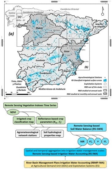
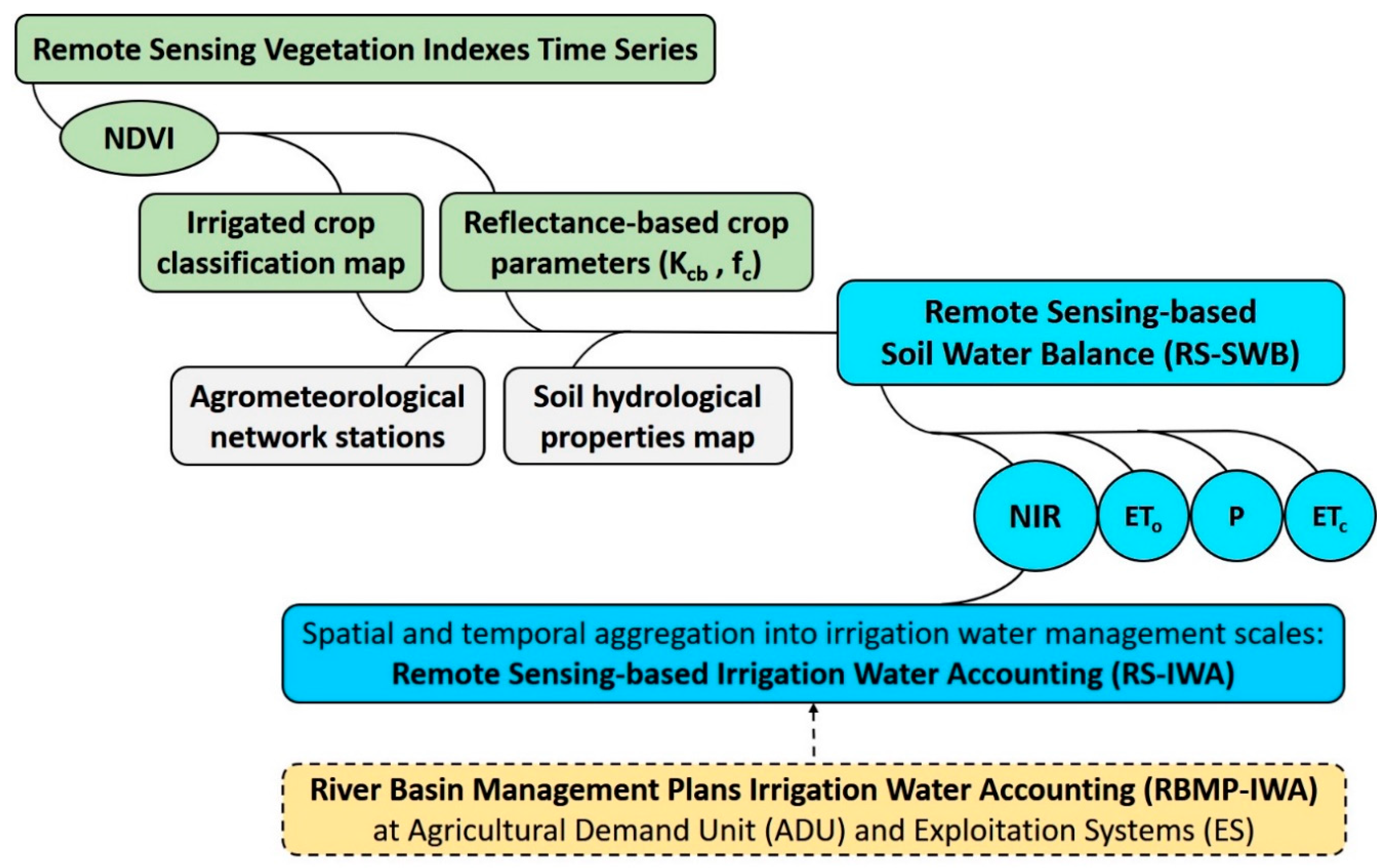
2.2. HidroMORE for Large Irrigation Areas

The RS-SWB (described in the following Section 2.3) was run using the latest version of the HidroMORE operational application to implement parallel processing with multithreading for running simulations over large areas [37]. Previously applied in different areas such as research [33,34,35,38,39,40], doctoral theses [41,42,43], and several research projects (SIRIUS EU project GA nº 262902, http://sirius-gmes.es/; DIANA EU project GA nº 703109, https://diana-h2020.eu/en/; CAPRA national Chilean project http://www.inia.cl/proyecto/502145/), HidroMORE spatially and temporally distributes the FAO56 model and integrates multispectral remote sensing data to provide the crop parameter evolution of the linear relationships between VI and both Kcb and the fraction of soil surface covered by vegetation (fc) [41]. Hence, using a pixel-by-pixel spatial scale and a daily temporal step (extended to the desired time range, such as x weeks, x months, x years, etc.), maps of the soil water balance variables are obtained as outputs from the model (i.e., ETo, P, ETc adj, and NIR), thereby producing an irrigation thematic cartography time series (Scheme 1). The set of satellite images used determines the total surface simulated, while the smallest spatial unit of work is the pixel size from the input satellite images. To implement the RS-SWB, HidroMORE uses the following input data: (a) VI time series, (b) a map of irrigated crops, (c) a map of soil types according to their hydrological properties, and (d) agroclimatic databases (daily P and ETo records).

2.2.1. VI Temporal Series

The normalized difference vegetation index (NDVI) was the VI selected to monitor crop evolution (see the justification in Section 2.3). While for the years of 2014 and 2015, the Landsat 8 satellite was used to process 938 scenes, during 2016–2018, the Sentinel-2 A and B satellites were selected to process 13,694 granules. Images were atmospherically corrected using an absolute normalization process [44], according to the selection of two different invariant surfaces to determine the NDVI linear regression values [45]. In addition, the inter-calibration of both satellites was achieved using coincident days to ensure the compatibility of the satellites with the NDVI time series over all the years. Moreover, as the selection of VI images is critical for correct irrigated crop monitoring, two criteria were followed: (i) selecting initial and final dates that covered the entire vegetative crop period and (ii) selecting images with the absence of clouds/shadows or images in which the presence of clouds/shadows could be correctly eliminated through masks and classification algorithms.
For the large and diverse irrigated surfaces monitored, the entire year was selected as the temporal date range. The final NDVI image selection after automatic cloud/shadow mask application was carried out through human supervision using the evolution of the VI time charts combined with colour RGB images loaded onto the SPIDERwebGIS® platform, which is specialized in handling such time series. The cloud/shadow classification algorithms varied according to the reference satellite used: (a) the Quality Assessment band for Landsat 8 (CFmask algorithm) and (b) the Sen2Cor algorithm for Sentinel-2 (http://step.esa.int/main/third-party-plugins-2/sen2cor/). The reliability of these algorithms was determined from different validation tests. The accuracy of CFmask in detecting clouds and shadows was around 90% [46], while for Sen2Cor, the precision results were around 80%, both for the high probability cloud classes and their shadows [47]. Despite these high values of cloud/shadow identification, difficulties remained in the correct classification of fine and high clouds [47], so time series monitoring was used to identify discontinuities and thus remove useless images.

2.2.2. Map of Irrigated Crops

The RS-SWB model applied by HidroMORE requires an annual map with the spatial distribution of the different irrigated crop classes to apply the methodology. Supported by official cartographic sources that facilitate the spatial delimitation assessment of irrigated areas (Common Agricultural Policy and ADU official cartography), these maps were constructed using a supervised multitemporal classification based on the VI thresholds, which require phenological cycle knowledge of the crops to be classified [48,49]. The final irrigated crop classes produced were spring, summer, spring–summer (double harvests), autumn–winter, and woody crops such as vineyards, olives, citrus, and fruit trees. Moreover, since crops with similar phenological and ground cover patterns have similar VI evolution and crop water requirements [48], the collected cycle was then used for the selection of threshold values for each type of irrigated crop class by VI time series at different phenological phases; these values are freely available on the project description website (see the Introduction section) and in the final report [50]. Hence, using these crop group classes and their VI profiles, we used the decision-tree approach on certain dates for crop class discrimination. The adopted classification facilitated the discrimination of the wide range of cultivated crops, as the crops were grouped according to the period within the year in which their phenological development takes place. Finally, the national irrigated surface area accounts according to previously described remote sensing approaches were proven and included by the Ministry for the Ecological Transition in an official report about the actual state of RBMPs at the national level [28].
HidroMORE uses specific information about each crop class to determine the soil water balance. The information collected in tables refers to the following parameters collected in FAO 56: the evapotranspiration depletion factor (p), the linear relationships of VI-Kcb and IV-fc, the maximum and minimum Kc values, the maximum and minimum root depth, the maximum and minimum VI, the water stress coefficient (Ks), and the irrigation period and irrigation dose per irrigation event.

2.2.3. Soil Hydrological Maps

The RS-SWB model applied by HidroMORE requires an annual spatially distributed map of soil hydrological properties. There are two sources for this map at the national scale [51,52]. However, none of these maps are digital. Hence, we used the map and database provided by the “European Soil Database Derived data” [53], which is mainly based on the “European Soil Database v2.0” [54] (E 1/1,000,000). This resource distributes open-source maps, including the total available water (TAW) and the maximum soil depth for root development, among other edaphological parameters.
These inputs are the most important for the necessary soil parameters to determine the cumulative net water depletion by roots in combination with the wilting point (θWP) and field capacity (θFC). The latter parameters are related with the provided TAW, so they are obtained from such information regarding the soil type knowing the TAW values. In addition, the soil evaporation from the exposed soil was modelled by applying the description of Torres and Calera [55] for the soil evaporation reduction coefficient and its correction factor under high evaporative rates, considering a depth of the surface soil layer of 0.1 m, as FAO56 recommends when the depth of the surface soil layer is unknown [10]. All this information is collected in tables that HidroMORE uses to run the RS-SWB.

2.2.4. Agrometeorological Databases

The RS-SWB model used with HidroMORE requires daily P and ETo data recorded by agrometeorological stations to spatially distribute the local information using the spatial interpolation (inverse distance weighting) of this local data. SIAR (the agrometeorological stations of the national network from the Agroclimatic Information System for Irrigation (http://www.siar.es/) of the Spanish Ministry of Agriculture, Food, and Fisheries) was used in combination with two regional agrometeorological networks (https://ruralcat.gencat.cat/web/guest/agrometeo.estacions and https://www.larioja.org/agricultura/es/informacion-agroclimatica/red-estaciones-agroclimaticas-siar). The annual average number of agrometeorological stations used was 536 (Figure 1a).

2.3. Remote Sensing-Based Irrigation Water Accounting for Large Areas

Remote Sensing-based Irrigation Water Accounting is the approach used to obtain the daily net irrigation requirements per pixel unit after applying a Remote Sensing-based Soil Water Balance to then spatially and temporarily aggregate these requirements to the desired work scale. The RS-SWB uses the well-known FAO56 methodology [10]. As expressed in Equation (1), this approach estimates the daily cumulative depth of evapotranspiration (depletion) from the root zone (Dr) that the crop extracts through adjusted crop evapotranspiration (ETc adj) in irrigation areas to subsequently apply a net irrigation depth (I) for the scenarios in which the precipitation (P) does not fully satisfy the crop water requirements. In parallel, as expressed in Equation (2) by the dual crop coefficient methodology [11], the ETc adj is estimated for the scenarios in which crops do not completely cover the ground surface (woody crops, horticultural crops, or herbaceous ones in the first stages) or require high irrigation frequency events (e.g., horticultural crops). Hence, the described crop development scenarios are common for large and diverse irrigation surface areas such as the present study area.
Dr i = Dr,i-1 − (P − RO)i − Ii − CRi + ETc adj,i + DPi
ETc adj,i = ETo · (Kcb · Ks + Ke)i
Avoiding the use of tabulated values for the basal crop coefficient (Kcb) or the fraction of soil surface covered by vegetation (fc) in large and diverse irrigation surface areas, the RS-SWB uses remote sensing capabilities to monitor crop evolution and obtain these crop parameters through dense VI time series [56,57] empirically derived from linear relationships (VI-Kcb act and VI-fc act). Besides focusing on operational applications, independent crop linear relationships are recommended [12,57,58,59]. For these reasons, and considering the ongoing debate on the use of independent VI linear relationships to estimate biophysical parameters, we selected the NDVI as the operative VI.
In this sense, Equation (3) expresses the linear relationship of the NDVI-Kcb selected [60]. Initially developed for vineyards, the NDVI-Kcb does not strongly differ from other published and evaluated linear relationships for maize [61,62] or sorghum [63] and was positively evaluated at different locations, such as vineyards in Chile [26] and Australia [64]; for different vegetation covers, such as savahan dehesa [65]; and in comparison with different VIs, such as the soil-adjusted vegetation index (SAVI) [66], in apple orchards [25]. In parallel, Equation (4) express the NDVI-fc linear relationship [67]. Originally developed for herbaceous crops such as maize and wheat, the NDVI-fc was applied to dry herbaceous and vineyards crops and as part of the RS-SWB to evaluate its reliability in soil water content estimations against ground truth data provided by ground sensors [40]. Moreover, the NDVI-fc was used in combination with other linear relationships to determine the spectral response evolution of maize and wheat, including the critical green-up step [68], and was evaluated to have good behaviour in comparison to ground measurements in vineyards [69].
Kcb act,i = 1.44 · (NDVI) − 0.1
fc act,i = 1.19 · (NDVI) − 0.16
Finally, at a daily frequency and pixel-based spatial unit scale, the RS-SWB inverts Equation (1) to obtain Equation (5). In this way, the NIR (mm/day) is estimated, producing thematic cartography for the temporally and spatially distributed balance applied. In this equation, the capillary rise (CRi) and superficial runoff (RO) were discarded. On the one hand, FAO56 does not recommend the use of CR when the water table is below 1 m from the soil surface [10] (a minority situation at the scale of the Iberian Peninsula) [70,71]. On the other hand, the RO was not computed by the HidroMORE software, as it was originally conceived for flat irrigation areas and works only with vertical fluxes, not lateral ones.
NIRi = (Dr,i-1 − Dr)i − P i + ETc adj, i + DP i
The methodological approach described above was positively evaluated at different irrigation management scales. At an annual temporal scale, along with three consecutive campaigns, the RS-IWA was compared with the ground truth data from commercial plots cultivated with wheat, barley, and maize and at the water user association management scale with a wide range of herbaceous crops and woody crops (mainly vineyards) [33]. Furthermore, the same approach was evaluated at a monthly temporal scale over four consecutive years and over a large irrigation surface area (about 100,000 ha, including herbaceous and woody crops) that is largely dependent on groundwater resources. The monthly groundwater withdrawal time series estimated by the RS-IWA were positively compared with strategically selected piezometric measurements from a piezometric network managed by the public authorities [34].

2.4. RBMP Irrigation Water Accounting Estimation (RBMP-IWA)

RBMPs are focused (among other objectives) on satisfying water demands, thereby rationalizing their use in harmony with the environment and other natural resources [31]. Thus, the knowledge of irrigation water demands is crucial for water demand management. However, due to the large extent of the territory that needs to be monitored and the high costs of the installation and maintenance of volumetric counters [72,73,74], the river basin authorities in Spain commonly determine water demands through spatially based indirect measurement approaches at the ADU, which is required by the national legal framework [30,31,32] as the minimum common spatial unit for irrigation water management in all Spanish RBMPs. The Hydrological Planning Offices are the public authorities in charge of this task, and large-scale efforts are made to combine different data sources to obtain the best estimations under the available resources. The 11 RBMPs consulted [75,76,77,78,79,80,81,82,83,84,85] followed similar approaches to irrigation water demand accounting, consisting of several sequential steps.
Firstly, the public water managers estimate the irrigable surface areas using sources such as the late national agricultural census (which dates from 2009), the surface related to water rights registration in the national private water registry (the variable dates for private water manager acquisitions), the information provided by the Common Agricultural Policy GIS (usually for the period 2010–2014), or, in some cases that do not cover the whole territory, RBD internal reports (based on field visits, regional surveys, or remote sensing techniques). In the second step, the proportion of crops or crop groups and their spatial distribution that covers the estimated irrigable surface areas are estimated by the public water managers. Again, the national agricultural census, the Common Agricultural Policy GIS, and regional surveys are the most common sources consulted. Thirdly, once the irrigable surface area and the proportion and distribution of crops or crop groups are estimated, the public water managers estimate the net irrigation water demand by multiplying the irrigable surface area proportion of each crop or crop group by their crop water requirements. The latter parameter relies on different data sources, such as the national recommendations provided in the ministerial law [30], which offer data ranges for parameters related to RBD spatial segmentation and crop or crop group division (i.e., 2900–7000 m3/ha·year in the Ebro RBD or 3400–6400 m3/ha·year in the Duero RBD for maize and sorghum, or 500–3350 and 1000–2900 m3/ha·year for the previous RBD in the case of winter cereals). However, previous recommendations are commonly complemented by and locally adapted with RBD internal reports based on local Irrigation Advisory Services that estimate the crop water demands in pilot areas. The fourth and final step consists of converting the estimated net irrigation water demands into gross irrigation water demands to account for the water that should be diverted to different irrigable surface areas. In this step, which is primarily based on national recommendations [30] and internal RBD reports, the Hydrological Planning Offices determine the irrigation efficiencies for the three irrigation water supply levels of application, distribution, and transport (i.e., 0.85–0.90 for open channel efficiency in the case of transport and distribution levels or 0.75–0.80 for the sprinkler application level) or a global efficiency coefficient that groups all levels.
For the previous approach, each Hydrological Planning Office fixes a base year for the irrigable surface areas and its probabilistic spatial crop distribution estimation over each ADU and then applies the crop water requirements and the irrigation efficiencies, thereby obtaining the irrigation water demand over large and diverse areas for this particular base year (in Spain, for the second hydrological planning cycle, the year of 2012 is commonly used). These values are then extrapolated to the next hydrological planning periods (2015–2021, 2021–2027, and so on) such that a unique yearly irrigation water demand value per ADU (or twelve values in the case of a monthly time scale) is used to cover all the years (or months) during the whole hydrological planning period (i.e., 2015–2021). The Hydrological Planning Offices extrapolate these values from the base year by considering future increments or decrements in the irrigable surface areas’ growth and/or planned investments for improving the irrigation efficiency of water user associations or irrigation water supply networks. As these changes do not quickly occur over such large and diverse areas, the differences between the estimated values for the base year and the following hydrological planning period are insignificant and only relevant for a few ADUs.
Note that the RBMPs group ADUs with similar characteristics into greater spatial scales called ESs, thereby allowing irrigation water management over greater scales. Besides the Duero RBD, a spatial unit smaller than the ADU is taken into consideration. Named the EDU, this unit is a subdivision of the ADU with common characteristics, such as the same water supply source.
Hence, considering the data available for the 11 RBMPs [75,76,77,78,79,80,81,82,83,84,85] at an annual temporal scale, the RBMPs publish the irrigation water demands of the ADU and ES and even, in some cases, at a monthly temporal scale for the ADUs. This public information was used at two spatial scales (ES and ADU) and, consequently, at two temporal scales (annual and monthly) in this research to compare the estimated RBMP-IWA with the results produced by RS-IWA.

2.5. RS-IWA Evaluation Approach in Comparison with RBMP-IWA at River Basin Spatial Scales

The daily NIR values estimated by RS-SWB at the pixel spatial scale were then spatially and temporally aggregated (RS-IWA) into the required water management scales that the RBMPs publish: monthly and annual temporal scales and EDU, ADU, and ES spatial scales (Section 2.4). Thus, by employing GIS spatial statistics (using Quantum GIS version 3.10 La Coruña), we obtained spatially and temporally distributed spatial statistics of the RS-IWA that were compared with RBMP-IWA (Scheme 1). The official cartography was directly downloaded from the RBD GIS viewers or RBD websites.
For the annual temporal scale, two irrigation water accounting comparisons are provided for the official period of 2015–2021 (named Annual estimated RBMP-IWA): (a) the annual sum for each study year to account for annual variability (named Annual RS-IWA) and (b) the annual average for the whole year dataset (named 5 year scale annual average RS-IWA) to bring the comparison closer to the published RBMP data (official value for the official period). For the monthly temporal scale, two irrigation water accounting comparisons are provided for the official period of 2015–2021 (named Monthly estimated RBMP-IWA): (a) the monthly sum for each study year to account for monthly variability (named Monthly RS-IWA) and (b) the monthly average over the whole year dataset (named 5 year scale monthly average RS-IWA) to bring the comparison closer to the published RBMP data (official value for the official period).
The statistical values used for the irrigation water accounting comparisons are the minimum (Min), maximum (Max), average (Av), standard deviation (σ), regression coefficient (r2), and Willmott refined index (dr) [86], which are commonly used in hydrological model evaluations. Both the absolute and relative values of the Root Mean Square Error (RMSE and RERMSE) and the Mean Absolute Error (MAE and REMAE) are also presented. However, although the RMSE is commonly used by researchers, the distribution and range of the comparison values in the present research work suggested the MAE to be the more representative of the two indexes [87].

3. Results

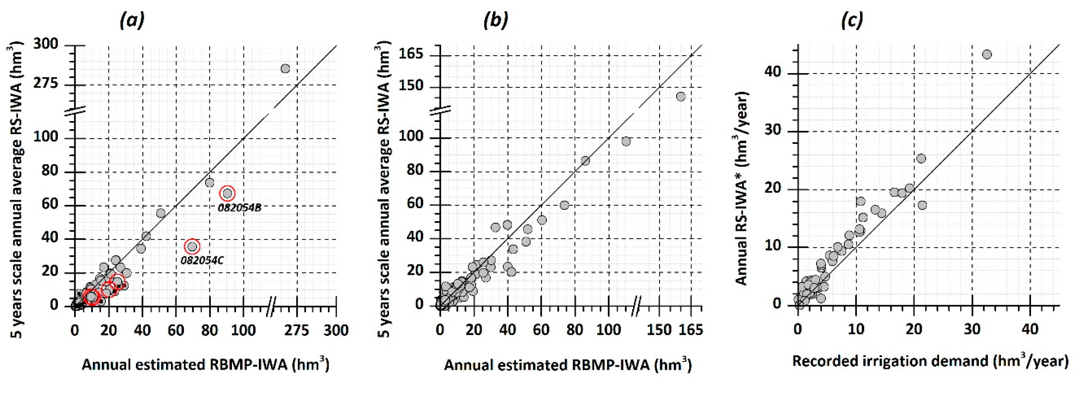
3.1. Annual RS-IWA Evaluation for Exploitation Systems in the Duero and Júcar RBDs

The daily NIR values obtained by the RS-SWB at a pixel-based spatial scale were then annually aggregated by their summation to compute the spatial statistics (described in Section 2.5) against the different ES irrigation water management spatial scales for the whole RBD in Júcar (9) and Duero (13) (Figure 1). Table 1 and Figure 2 show the irrigation water accounting comparison. While the Júcar RBD provides the net annual irrigation water demands in the RBMP, the Duero RBD provides the annual gross irrigation water demands; thus, to provide a coherent comparison between the published data and the model results, the global irrigation efficiency coefficient of 0.62, published by Duero RBMP, was used to convert the gross irrigation water demands into the net irrigation water demands. Furthermore, the irrigable surface areas estimated by the RBMP were compared with the irrigated surface areas estimated by the RS-SWB.
The 5 year scale annual average RS-IWA comparison with the official values for the 2015–2021 period showed a strong regression coefficient r2 for both the Duero and Júcar RBDs (0.95 and 0.99, respectively), as well as a strong Willmott refined index dr (0.88 and 0.93, respectively). In that sense, the REMAE provided values of 20% and 15% for the Duero and Júcar RBD, respectively. Case by case, the majority of the comparison values for the ESs in the Duero RBD showed a slight underestimation. However, this was not the case for the Júcar RBD, except for the Vinalopó–Alacantí ES. The latter case showed a larger underestimation, which, under our criteria, was based on the following: (a) the comparison between the irrigable surface area (RBMP) and irrigated surface area (RS-SWB) presented a larger negative relative error (−56%) compared to the other Júcar ESs, revealing many surface areas not considered by remote sensing techniques in this ES, and (b) the Júcar RBMP estimated a large irrigable surface area for successive annual crops (double harvest groups) with consequently high irrigation water demand estimations by the Hydrological Planning Offices. However, in this study, the crop classification for this area did not reveal an important surface for double harvest crop classes but did reveal an important surface for spring and summer classes (i.e., there was less irrigation water demand than that for the double harvest group). Even so, this underestimation does not invalidate the good r2 and dr agreement reached in this RS-IWA evaluation due to its low statistical weight compared to the other ESs.
For the Annual RS-IWA, the results show that the model captures annual variability based on the average, minimum, and maximum values in different years for each RBD. For example, the years of 2015 and 2017 in the Duero RBD present the highest values, indicating the years with higher irrigation water demands according to remote sensing, while the same phenomena are present in the Júcar RBD for the years of 2014 and 2016.

3.2. Annual RS-IWA Evaluation Regarding Agricultural Demand Units in Duero and Júcar RBDs

The daily NIR obtained by the RS-SWB at a pixel-based spatial scale were then annually aggregated by their summation to compute the spatial statistics (described in Section 2.5) against the different ADUs’ irrigation water management spatial scales for the whole RBD in Júcar (98) and Duero (290) (Figure 1b,c). Table 2 and Figure 3a,b show the irrigation water accounting comparisons. While the Júcar RBD provides the net annual irrigation water demand in the RBMP, the Duero RBD provides the annual gross irrigation water demand. Thus, one irrigation efficiency coefficient for each ADU in the Duero RBD (provided by the RBMP) was compared against the RS-IWA values.
The 5 year scale annual average RS-IWA comparison with the official values for the 2015-2021 period again shows a strong regression coefficient r2 of 0.96 for both the Duero and Júcar RBDs, as well as a strong Willmott refined index dr (0.90 and 0.88, respectively). The REMAE shows values of 26% and 28% for the Duero and Júcar RBDs, respectively. At this spatial scale, a common underestimation was observed for both RBDs. Hence, we highlight several ADUs in the Júcar RBD comparison in Figure 3a. The first group (black squares in Figure 3a) is represented by four ADUs, all located in the Vinalopó–Alacantí ES (082073A, 082075A, 082076A, and 092001A), that demand 84% of the irrigation water resources in this ES and were underestimated by the RS-IWA according to previous observations (commented in Section 3.1). The second group (red circles in Figure 3a) contains six ADUs (082034C, 082034D, 082054B, 082054C, 082054D, and 082054E) in which rice is the majority crop cultivated. In these ADUs, the RS-IWA underestimated the irrigation water demands by about 50% for the RBMP-IWA, except for the ADU 082054B, for which a 25% lower irrigation water demand was estimated by the RS-IWA. The difference between these two subgroups relies on their rice surface irrigation areas because, for the latter ADU, the proportion of rice is just 20%, compared to the other five ADUs, where the rice proportion is between 50 and 100%.
For the annual RS-IWA comparison, the model collects annual variability as observed previously in the ES spatial scale. However, in this case, we highlight the minimum values—i.e., the years with less irrigation water demands determined by the RS-IWA for both RBDs in 2016 and 2018.
Besides the annual irrigation water demands estimated by the Duero RBMP, annual monitoring measurement reports are available along three consecutive hydrological year (October to September for 2015–2016, 2016–2017, and 2017–2018) for the water consumed at the EDU spatial scale. Choosing the EDUs with a maximum bias of 20% between the irrigable and irrigated surface areas to use comparable data, we ultimately selected 49 EDUs. Figure 3c shows the irrigation water accounting comparison between the recorded measurements and the annual RS-IWA* (recomputed at annual temporal scales considering the hydrological year). The statistical analysis reveals results similar to previous findings, with a regression coefficient of r2 = 0.94, a Willmott refined index of dr = 0.81, and an REMAE of 24% (MAE = 2 hm3).

3.3. Monthly RS-IWA Evaluation of Agricultural Demand Units in the Júcar and Duero RBDs

The daily NIR obtained for the RS-SWB at a pixel-based spatial scale were then aggregated monthly by their summations to compute the spatial statistics (described in Section 2.5) for the different ADU irrigation water management spatial scales for the whole RBDs in Júcar (98) and Duero (290) (Figure 4). While the Júcar RBD provides the annual net irrigation water demand in the RBMP, the Duero RBD provides the annual gross irrigation water demand; thus, the irrigation efficiency coefficient for each ADU in the Duero RBD was compared against the RS-IWA values. The r2 and dr monthly time series are also represented in the figure.
Both time series for the 5 year scale monthly average RS-IWA and the Monthly RS-IWA follow similar monthly temporal patterns in their monthly estimated RBMP-IWA. In that sense, the maximum values are observed in spring or summer, while the minimum values occur in autumn and winter. However, for both RS-IWA time series, underestimations are common for all the years, especially in summer, while for some spring and autumn months, higher values were estimated. These values reflect time series decoupling for autumn in both RBDs, which is clearer in the Duero RBD, where higher monthly RS-IWA values are constant over the 5 years; therefore, the 5 year scale monthly average RS-IWA reflects this overestimation. Conversely, in the Júcar RBD, slight overestimations occur in spring.
For the monthly evolution of the statistical index, we observed strong results for the r2 and dr (about 0.9 and 0.8, respectively) in months where more irrigation water resources are consumed—i.e., during the central months of irrigation campaigns in both RBDs, mainly April to September. However, these values strongly decrease in the winter months, when the minimum water resources are consumed for the monthly estimated RBMP-IWA, yielding r2 values close to 0.0, especially in the Duero RBD, which also has dr monthly values close to −1.0. In the Júcar RBD, during the winter months, the statistical values are slightly higher than those in the Duero RBD. These results are related to the minimum (or absence, as in the Duero RBD) of irrigation water demand estimations from the RBMP. Hence, the comparison shows a remarkably similar numerical data range, albeit with a very low dispersion. Thus, while statistically speaking, r2 values close to zero show no correlation, mathematically speaking (and according to the r2 formulation), an output of values close to zero makes sense.
In addition to Figure 4, which shows the global situation in the RBDs according to the monthly irrigation water accounting and considering all the ADUs, Figure 5 shows the same irrigation water accounting time series but for the specific ADUs demanding the highest irrigation water volumes and belonging to different ESs. We included three ADUs per RBD: one of them principally depends on groundwater resources (Mancha Oriental and Bombeo Medina del Campo), while the other two depend greatly on surface water resources. Moreover, the monthly P and ETo values from the closest agrometeorological stations using the SIAR network were plotted. Including these climatic variables helps to explain the monthly variability of the RS-IWA.
Again, the maximum and minimum tendency values agree for both RS-IWA estimations in the monthly estimated RBMP-IWA. However, on a smaller scale and in response to climatic conditions, the RS-SWB shows variations in the estimation of the irrigation water demands when comparing the same months in different years (for example, May). Seasonal decoupling that does not manifest in other years is also observable for specific years (particularly in spring and autumn). In that sense, decoupling is also observable in the spring and autumn months. The highest decoupling was found every year for both of the ADUs with groundwater resource dependency, Mancha Oriental (Júcar RBD) and Bombeo Medina del Campo (Duero RBD). While the former ADU always reaches its monthly RS-IWA maximum values in spring, like the monthly estimated RBMP-IWA, in the latter case, these values are distributed in the spring and autumn seasons. Moreover, the RS-IWA distributes its maximum values over the summer months, while the RBMP-IWA estimates its maximum values in June.
For the statistical indices, we found strong r2 agreements for ADUs with a superficial origin of water resources (between 0.89 and 0.94), which are much lower for ADUs with groundwater resource origins (0.66 in Medina del Campo and 0.49 for Mancha Oriental). In the same way, we observed stronger dr agreements for ADUs with superficial water resources (between 0.86 and 0.91) and the weakest ones for ADUs with groundwater resources (0.72 and 0.63, respectively).

3.4. Annual RS-IWA Evaluation for the ES Spatial Scale for the 11 RBDs in Mainland Spain

The daily NIR obtained by the RS-SWB at a pixel-based spatial scale were then annually aggregated by their summation to compute the spatial statistics (described in Section 2.5) for the different ES irrigation water management spatial scales of the 11 RBDs under study (four in GDN, one in SEG, two in GyB, one in TOP, five in CMA, four in CIC, five in TAJ, 13 in DUE, eight in GDQ, 17 in EBR, and nine in JCR). Table 3 and Figure 6 show the irrigation water accounting comparison. In the eight RBDs (TAJ, GDN, SEG, CMA, GyB, DUE, GDQ, and JCR), the global RBD efficiency coefficient was available, so the annual net irrigation water demands were computed. However, for the other RBDs, we did not find this coefficient, so we used the average value of these eight RBDs (a range of values between 0.41 and 0.81, with an average of 0.68) to convert the annual gross irrigation water demand estimations into their net values.
Figure 6a shows strong agreements for r2 = 0.91 and dr = 0.84 in the comparison between the 5 year scale annual average RS-IWA and the annual estimated RBMP-IWA. However, the REMAE returns 41% (Table 3), which is clearly influenced by the annual REMAE of 62% returned for 2018 in comparison with the four preceding years, where the REMAE ranged from 30 to 45%. For the annual variability returned by the annual RS-IWA, the year of 2015 has the highest irrigation water demands, even larger than the annual estimated RBMP-IWA, while 2018 has the lowest. In terms of irrigation and irrigated surface area comparisons (Figure 6b), the statistical indices for each year separately, as well as the 5 year average, show good agreement, with an r2 in the range of 0.95 to 0.98 and a dr of 0.86 to 0.88. In that sense, the REMAE ranges from 27 to 34%, so any year could be highlighted as the best one.
Figure 6 shows five ESs highlighted with red circles showing high under- or overestimations of the 5 year scale annual average RS-IWA, in contrast with published data on the annual estimated RBMP-IWA. Hence, in the four ESs (the Segura ES in SEG RBD, Regulación General ES in GDQ RBD, Sierra Nevada ES in CMA RBD, and Bajo Ebro ES in EBR RBD), the RS-SWB strongly underestimates the annual RS-IWA, with one high overestimation (Oriental ES in TAJ RBD). These four ESs also underestimate the irrigated surface area. These findings support the idea that the irrigated surface area determines good agreement for irrigation water accounting. However, a deeper analysis reveals important ES characteristics that deserve analysis.
Underestimation of 620 and 460 hm3/year was detected in the two ESs selected (Bajo Ebro (EBR RBD) and Regulación General (GDQ RBD), respectively), where the rice crop surfaces are presented as about 30,000 and 40,000 ha. As mentioned previously for the six ADUs from the Júcar RBD with rice crop surfaces (Section 3.2), a new and highlighted underestimation was revealed for such crops. A different situation was revealed in the Sierra Nevada ES (CMA RBD), where horticultural crops under greenhouse conditions were the predominant crops (the El Ejido zone, Almería). Hence, with a surface of about 27,000 ha (60% of the irrigable surface area estimated by the RBMP), an underestimation of 230 hm3/year was obtained. However, the NIR of this crop group cannot be simulated by the RS-SWB, as the spectral response from the satellite for greenhouses is linked to the plastic cover, not to crop development. Moreover, the other three ESs that comprise the CMA RBD also feature greenhouses, although not as densely, so underestimation is not as great as that for the aforementioned ES. The last selected underestimation is linked with horticultural crops in successive harvesting during the year, as is the case for the Segura ES (SEG RBD). The RBMP estimated around 50% of the irrigable surface area dedicated to this goal, while the supervised classification did not reveal such a figure, instead indicating mainly spring and summer crops. Therefore, the underestimation of about 450 hm3 was related to an incorrect classification and, consequently, poor crop RS-SWB parametrization, while the RBMP estimates irrigation water demands considering several successive crop harvests in the same year.
On the other hand, we observed an overestimation (about 280 hm3) for the Oriental ES (GDN RBD). Although the irrigated surface area returned by the RS-SWB was slightly higher than the irrigable surface area estimated by the RBMP, we believe that the annual estimated RBMP-IWA is restricted because in the ES, the irrigated agriculture is groundwater-dependent, and the aquifer is classified as overexploited.

4. Discussion

The present research evaluated the RS-IWA’s reliability over large and diverse irrigation surface areas. Using the FAO56 approach and remote sensing images, an RS-SWB was applied to estimate the NIR at a daily temporal scale and a pixel-based spatial scale. The spatially distributed thematic cartography generated was then aggregated into the same spatial and temporal irrigation water management scales that public managers use for water management expressed in the RBMPs. Therefore, the RS-IWA was evaluated over three spatial scales (EDU, ADU, and ES) and two temporal scales (annual and monthly) using the official irrigation water demands published in the RBMPs.
The spatial adaptability of the NIR thematic cartography to a desired spatial management scale depends on the original satellite images’ spatial resolutions. In that sense, for 2014 and 2015, the present research used 30 m-scale satellite Landsat 8 data, while for 2016–2018, we used 10 m-scale data from the twin satellites of Sentinel-2 (A and B). In parallel, the temporal adaptability to the desired temporal management scale depends on the product’s temporal frequency generation. Thus, the RS-SWB operates with a daily time step using dense satellite VI time series to allow adequate crop evolution monitoring. Both irrigation management working scales are appropriate for irrigation water monitoring with different plot shapes and sizes [88], including Sentinel-2 products for precision agriculture [89]. Moreover, the temporal and spatial scales produced agree with different and actual remote sensing operative applications, such as ALEXI/DisALEXI, which generates daily evapotranspiration products up to a 30 m spatial scale [14]; MINARET, which annually estimates daily unstressed crop evapotranspiration at a 30 m spatial scale along the Guadalquivir RBD for water management purposes; and the daily TOP-SIMS maps in California on basal crop evapotranspiration, among other products, at a 30 m spatial scale.
To date, ETc has been commonly used to evaluate models over irrigation surface areas [90,91,92,93,94], as has the Crop Water Requirements approach [17,24,95]. However, increasingly, studies use the irrigation water volume, both the estimation and value recorded at the field plot level, to evaluate models over irrigation surface areas [26,96,97]. In this vein, the present research used NIR as a variable to evaluate the RS-IWA based on different criteria. On the one hand, there is no distributed instrument network for in situ ETc measurements [72] that can supply the required ground truths for the different irrigation management spatial scales used by water authorities. On the other hand, we can use the same magnitudes and products that water authorities publish in their RBMPs after their estimation by the Hydrological Planning Offices based on the best resources and tools available to these water managers. Thus, published data (without being strictly ground truths, since many data are estimations) play a legal role, whose numerical values are used as a reference for irrigation water management during each hydrological planning cycle. Therefore, the presented approach provides irrigation water accounting assisted by remote sensing, and the variables used to validate them represent a form of novelty. Recent work shows that similar procedures have already used data from water authorities and remote sensing to assess irrigation water requirements over large areas and provide recommendations such as for several River Basins located in Jordan [98] or the Tarim River Basin in China [99].
The RS-IWA evaluation was satisfactory at different temporal and spatial scales. The agreement indexes r2 and dr returned positive values within the range of 0.79–0.99, except for the winter season, when the agreement indexes were closer to zero when evaluated at the monthly time scale (nevertheless, these findings are not statistically representative, as already explained in Section 3.3). Furthermore, the REMAE maintained ranges of 11–40% in 28 of the 31 conducted evaluations, which is in line with the similar range of about 15–40% for typical errors when ETc is computed through the VI [22]. We used these ranges like qualitative indicators because their variables are not the same. Finally, we also highlighted the EDU spatial scale for the Duero RBD because the annual RS-IWA* evaluation compared to the ground truth volumetric measurements returned good results (r2 = 0.94, dr = 0.81, and REMAE = 24%), which were in line with similar findings produced (good agreements and RMSE of about 15%) by the same model over three consecutive years at the plot and water management user scales in a different location [33].
The presented operational approach incorporates annual and monthly climatic dynamics, mainly, the annual/monthly RS-IWA product, which corresponds to the precipitation recorded at different spatial scales and is in line with other research’s crop water requirement estimations [100,101]. Conversely, the 5 year scale annual/monthly average RS-IWA product was used to aggregate these climatic dynamics to incorporate successive study years. Thus, according to the seasonal and annual climatological reports (http://www.aemet.es/es/serviciosclimaticos/vigilancia_clima/resumenes) by the Spanish Meteorological Agency along with the present research work, two years were considered wet (2014 and 2016, with 680 and 682 mm, respectively, of annual precipitation), one year was very wet (2018, with 808 mm), and two more years were classified as dry years (2015 and 2017, with 500 and 474 mm, respectively). This annual variability was incorporated into the RS-SWB (Table 3), returning lower annual RS-IWA values for wet years and higher ones for dry years, which suggests that the annual RS-IWA is more accurate for the RBMP-IWA when a dry year occurs. In parallel, the behaviour of the monthly RS-IWA is similar, as expected based on previous findings. Therefore, the RS-SWB model incorporates monthly variability, as shown in Figure 5, from particular ADUs in the Duero and Júcar RBDs, where the lower irrigation water demand estimations respond to higher precipitation (i.e., June 2018) and vice versa, including the decoupling of the monthly RS-IWA time series for the RBMP-IWA. Such monthly temporal mismatching between remote sensing and official water managers’ approaches have been observed in similar studies in the case of the Doukkala region in Morocco [100] or the Haihe Plain in China [102].
For the RS-IWA spatial scale aggregation following the deep evaluation conducted over the Júcar and Duero RBDs, the results did not show strong evidence for which spatial scale provides better results. The REMAE at the EDU and ADU spatial scales varied from 24 to 43%, providing slightly better results in the ES spatial scale (with a range of 11–37%). However, when increasing the study area to 69 ESs over the 11 RBDs, good agreement indexes were found, but the REMAE for the product of the 5 year scale annual average RS-IWA was about 41% (because the year 2018 returned a 61% REMAE value, in contrast with the average value of 38%, considering the previous four study years, which is in agreement with the worst RS-IWA results being found for wet years). At this spatial scale, as noted in Section 3.4, the underestimations that trigger a higher REMAE are linked with ESs containing a high proportion of rice crops, greenhouses, or successive horticultural crops each year.
Moreover, such improvements are already available. The spatial locations of rice crops are correctly defined by the Common Agricultural Policy GIS, so actual public water methodologies from the RBMP methodology can be used to estimate the irrigation water demands. However, considering the remote sensing benefits of monitoring crop developments in near real time, we could use the operational approach of González-Dugo et al. [103] (applied using MINARET) to obtain rice crop extensions followed by the application of other vegetation indices, such as the SAVI, to estimate unstressed crop evapotranspiration (using certain adapted crop parameters), among other approaches.
In parallel, the horticultural crops under successive harvesting located in the Segura ES from the SEG RBD can be correctly monitored by remote sensing using the high temporal resolution provided by the twin satellites of Sentinel-2 (A and B). In this sense, recent research applying Random Forest classification approaches returned good results for carrot, pumpkin, and onion classifications [104]. However, we must bear in mind the diverse crop types under this crop group and the different strategies of farming using different water management approaches [105]. Consequently, aggregating all these elements into one group class will require further research to maintain an easy and operational methodology. Finally, the classification of greenhouses could be achieved using many recent advances by applying Sentinel-2 [106,107]. However, the RS-IWA under greenhouses remains a limitation for the methodology presented here because optical satellites are not able to monitor such crops.

5. Conclusions

Presently, operational applications in irrigated areas based on remote sensing techniques are available. Thus, enlarged remote sensing applications over large and diverse irrigation surface areas would offer public and private water managers a complementary tool for obtaining information and satisfy the European requirements at the Water Framework Directive level. In this sense, the good agreement reached between the RS-IWA evaluation and the RBMP-IWA data estimated by the Hydrological Planning Offices and published in the RBMP satisfies the initial objective of presenting a simple, homogeneous, and reproducible operational tool for large and diverse irrigation surface areas. Moreover, the thematic cartography is characterized by having great adaptability to the spatial and temporal irrigation water management scales used by water managers, so NIR maps are applicable at any management level.
Consequently, several RS-IWA products were introduced. First, the 5 year scale annual/monthly average RS-IWA, which aggregates the temporal behaviour of agroclimatic and agricultural strategies over five study years, is suggested for use when medium-/long-term accounting is required, such as for the six-hydrological-year cycle. Secondly, the annual/monthly RS-IWA, which incorporates variable climatological conditions and allows one to monitor the actual values of NIR, can be used to improve annual or monthly irrigation water resource monitoring.

Author Contributions

J.G.-R. and A.C. conceived and designed the methodology; M.B. and L.F. processed the satellite images; I.A., L.F. and J.G.-R. classified the surface irrigation areas; J.G.-R. run the RS-SWB; R.B. and T.O. supervised and analyzed the project results; J.G.-R. and J.G.-P. processed and analyzed the RS-IWA data; J.G.-R. and J.G.-P. wrote, reviewed and edited the manuscript. All authors have read and agreed to the published version of the manuscript.

Funding

The work was funded by the project named SPIDER-SIAR [27,28,29,30] by the Deputy Directorate General for Irrigation and Water Economy of the Spanish agricultural ministry. It was developed during 2014–2018 in mainland Spain. Its results, thematic cartography, and methodological reports are freely available from the SPIDERwebGIS®, SPIDER-SIAR group (http://maps.spiderwebgis.org/login/?custom=spider-siar).

Acknowledgments

The authors acknowledge the Hydrological Planning Offices who are presently studying and analyzing the thematic cartography supplied, as well as the project funding for acquiring deeper knowledge with new approaches and tools over large and diverse irrigation surface areas.

Conflicts of Interest

The authors declare no conflict of interest.

Acronyms

ADU Agricultural Demand Unit
EDU Elemental Demand Unit
NIR Net Irrigation Requirements
RBD River Basin District
RBMP River Basin Management Plan
RS-IWA Remote Sensing-based Irrigation Water Accounting
RS-SWB Remote Sensing-based Soil Water Balance
ES Exploitation System

References

  1. AQUASTAT Website. AQUASTAT—FAO’s Information System on Water and Agriculture. Available online: http://www.fao.org/nr/water/aquastat/water_use/index.stm (accessed on 1 September 2020).
  2. EEA Water Resources across Europe—Confronting Water Scarcity and Drought—European Environment Agency. 2019. Available online: https://www.eea.europa.eu/publications/water-resources-across-europe (accessed on 27 September 2020).
  3. The Council of the European Union. Directive 2000/60/EC of the European Parliament and of the Council of 23 October 2000 Establishing a Framework for Community Action in the Field of Water Policy; The Council of the European Union: Brussels, Belgium, 2000; Volume L327, pp. 1–82. [Google Scholar]
  4. European Commission. Introduction to the EU Water Framework Directive—Environment—European Commission. Available online: https://ec.europa.eu/environment/water/water-framework/info/intro_en.htm (accessed on 1 September 2020).
  5. European Commission. European Overview—Second River Basin Management Plans 5th Implementation Report; European Environmental Bureau (EEB): Brussels, Belgium, 2019. [Google Scholar]
  6. Del Cura, C.M.; Ramírez, J. Influencia de la Calidad del Agua en la Metrología de los Contadores de Riego. XXIX Congreso Nacional de Riegos. 2011. Available online: http://www.aeryd.es/empresas/aeryd/trabajos/2011-C-20.pdf (accessed on 27 September 2020).
  7. Pérez, J.; del Cura, C.M.; de Ribera, A.S. Influencia en la Disposición de un Contador en su Metrología. XXIX Congreso Nacaional de Riegos. 2011. Available online: http://www.aeryd.es/empresas/aeryd/trabajos/2011-C-19.pdf (accessed on 27 September 2020).
  8. Papadakis, D.; Milosavljevic, I. Copernicus Sentinel Benefits Study. Exploring Sectoral Uptake of Sentinel Data within Academic Publications. 2019. Available online: http://0-earsc-org.brum.beds.ac.uk/Sebs/wp-content/uploads/2019/07/CopernicusSentinelBenefitsStudy_UptakeOfSentinelDataInAcademicPublications_June2019.pdf (accessed on 8 July 2020).
  9. Serbina, L.; Miller, H.M. Landsat and Water—Case Studies of the Uses and Benefits of Landsat Imagery in Water Resources; U.S. Geological Survey Open-File Report. 2014–1108; U.S. Geological Survey: Reston, VA, USA, 2014; 61p. [Google Scholar] [CrossRef]
  10. Allen, R.G.; Pereira, L.S.; Raes, D.; Smith, M. Crop Evapotranspiration—Guidelines for Computing Crop Water Requirements. Available online: http://www.fao.org/3/X0490E/x0490e00.htm (accessed on 1 September 2020).
  11. Wright, J. New evapotranspiration crop coefficients. J. Irrig. Drain. Div. 1982, 108, 57–74. Available online: https://eprints.nwisrl.ars.usda.gov/id/eprint/382 (accessed on 27 September 2020).
  12. Calera, A.; Campos, I.; Osann, A.; D’Urso, G.; Menenti, M. Remote sensing for crop water management: From ET modelling to services for the end users. Sensors 2017, 17, 1104. [Google Scholar] [CrossRef] [PubMed] [Green Version]
  13. Bastiaanssen, W.G.M.; Menenti, M.; Feddes, R.A.; Holtslag, A.A.M. A remote sensing surface energy balance algorithm for land (SEBAL). 1. Formulation. J. Hydrol. 1998, 212–213, 198–212. [Google Scholar] [CrossRef]
  14. Anderson, M.C.; Kustas, W.P.; Norman, J.M.; Hain, C.R.; Mecikalski, J.R.; Schultz, L.; González-Dugo, M.P.; Cammalleri, C.; D’urso, G.; Pimstein, A.; et al. Mapping daily evapotranspiration at field to continental scales using geostationary and polar orbiting satellite imagery. Hydrol. Earth Syst. Sci. 2011, 15, 223–239. [Google Scholar] [CrossRef] [Green Version]
  15. Allen, R.G.; Tasumi, M.; Trezza, R. Satellite-based energy balance for Mapping Evapotranspiration with Internalized Calibration (METRIC)—Model. J. Irrig. Drain. Eng. 2007, 133, 380–394. [Google Scholar] [CrossRef]
  16. D’Urso, G.; Menenti, M.; Santini, A. Regional application of one-dimensional water flow models for irrigation management. Agric. Water Manag. 1999, 40, 291–302. [Google Scholar] [CrossRef]
  17. Vuolo, F.; D’Urso, G.; De Michele, C.; Bianchi, B.; Cutting, M. Satellite-based irrigation advisory services: A common tool for different experiences from Europe to Australia. Agric. Water Manag. 2015, 147, 82–95. [Google Scholar] [CrossRef]
  18. Kanemasu, E.T. Seasonal canopy reflectance patterns of wheat, sorghum, and soybean. Remote Sens. Environ. 1974, 3, 43–47. [Google Scholar] [CrossRef]
  19. Trout, T.; Johnson, L.; Gartung, J. Remote sensing of canopy cover in horticultural crops. HortScience 2008, 43, 333–337. [Google Scholar] [CrossRef] [Green Version]
  20. Jackson, R.D.; Huete, A.R. Interpreting vegetation indices. Prev. Vet. Med. 1991, 11, 185–200. [Google Scholar] [CrossRef]
  21. Bausch, W.C. Remote sensing of crop coefficients for improving the irrigation scheduling of corn. Agric. Water Manag. 1995, 27, 55–68. [Google Scholar] [CrossRef]
  22. Allen, R.G.; Pereira, L.S.; Howell, T.A.; Jensen, M.E. Evapotranspiration information reporting: I. Factors governing measurement accuracy. Agric. Water Manag. 2011, 98, 899–920. [Google Scholar] [CrossRef] [Green Version]
  23. Choudhury, B.J.; Ahmed, N.U.; Idso, S.B.; Reginato, R.J.; Daughtry, C.S.T. Relations between evaporation coefficients and vegetation indices studied by model simulations. Remote Sens. Environ. 1994, 50, 1–17. [Google Scholar] [CrossRef]
  24. D’Urso, G.; Richter, K.; Calera, A.; Osann, M.A.; Escadafal, R.; Garatuza-Pajan, J.; Hanich, L.; Perdigão, A.; Tapia, J.B.; Vuolo, F. Earth observation products for operational irrigation management in the context of the PLEIADeS project. Agric. Water Manag. 2010, 98, 271–282. [Google Scholar] [CrossRef]
  25. Odi-Lara, M.; Campos, I.; Neale, C.M.U.; Ortega-Farías, S.; Poblete-Echeverría, C.; Balbontín, C.; Calera, A. Estimating evapotranspiration of an apple orchard using a remote sensing-based soil water balance. Remote Sens. 2016, 8, 253. [Google Scholar] [CrossRef] [Green Version]
  26. Balbontín, C.; Campos, I.; Odi-Lara, M.; Ibacache, A.; Calera, A. Irrigation performance assessment in table grape using the reflectance-based crop coefficient. Remote Sens. 2017, 9, 1276. [Google Scholar] [CrossRef] [Green Version]
  27. Pereira, L.S.; Alves, I. Crop water requirements. In Reference Module in Earth Systems and Environmental Sciences; Elsevier: Amsterdam, The Netherlands, 2013. [Google Scholar] [CrossRef]
  28. Directorate-General of Water, Secretary of State for the Environment, M. for the E.T.; Hydrographic Studies Centre, Centre for Public Works Studies and Experimentation (CEDEX), Ministry of Public Works, M.; Transition, for the E. Summary of Spanish River Basin Management Plans. Second Cycle of the WFD (2015–2021). Available online: https://www.miteco.gob.es/es/agua/temas/planificacion-hidrologica/summary_book_rbmp_2nd_cycle_tcm30-508614.pdf (accessed on 27 September 2020).
  29. Spanish Ministry of Agriculture, Fisheries and Food. Encuesta de Superficies y Rendimientos de Cultivos. Informe Sobre Regadíos en España. 2019. Available online: https://www.mapa.gob.es/es/estadistica/temas/estadisticas-agrarias/boletin2019_tcm30-536911.pdf (accessed on 29 July 2020).
  30. MMA (Ministerio de Medio Ambiente). Instrucción de Planificación Hidrológica. Available online: https://www.boe.es/eli/es/o/2008/09/10/arm2656/con (accessed on 1 September 2020).
  31. MMA (Ministerio de Medio Ambiente). Texto Refundido de la Ley de Aguas. Available online: https://www.boe.es/eli/es/rdlg/2001/07/20/1/con (accessed on 1 September 2020).
  32. MMA (Ministerio de Medio Ambiente). Reglamento de la Planificación Hidrológica. Available online: https://www.boe.es/eli/es/rd/2007/07/06/907/con (accessed on 1 September 2020).
  33. Garrido-Rubio, J.; González-Piqueras, J.; Campos, I.; Osann, A.; González-Gómez, L.; Calera, A. Remote sensing–based soil water balance for irrigation water accounting at plot and water user association management scale. Agric. Water Manag. 2020, 238, 106236. [Google Scholar] [CrossRef]
  34. Garrido-Rubio, J.; Sanz, D.; González-Piqueras, J.; Calera, A. Application of a remote sensing-based soil water balance for the accounting of groundwater abstractions in large irrigation areas. Irrig. Sci. 2019, 37, 709–724. [Google Scholar] [CrossRef]
  35. Garrido-Rubio, J.; Calera, A.; Enguita, L.F.; Alcázar, I.A.; Mancebo, M.B.; Rodríguez, I.C.; Rubio, R.B. Remote sensing-based soil water balance for irrigation water accounting at the Spanish Iberian Peninsula. Proc. Int. Assoc. Hydrol. Sci. 2018, 380, 29–35. [Google Scholar] [CrossRef] [Green Version]
  36. Köppen, W.; Geiger, R. Handbuch der Klimatologie in fünf Bänden Das geographische System der Klimate; Borntraeger: Berlin, Germany, 1936. [Google Scholar]
  37. Moreno, R.; Arias, E.; Sanchez, J.L.; Cazorla, D.; Garrido, J.; Gonzalez-Piqueras, J. HidroMORE 2: An optimized and parallel version of HidroMORE. In Proceedings of the 2017 8th International Conference on Information and Communication Systems (ICICS), Irbid, Jordan, 4–6 April 2017; pp. 1–6. [Google Scholar] [CrossRef]
  38. Sánchez, N.; Martínez-Fernández, J.; González-Piqueras, J.; González-Dugo, M.P.; Baroncini-Turrichia, G.; Torres, E.; Calera, A.; Pérez-Gutiérrez, C. Water balance at plot scale for soil moisture estimation using vegetation parameters. Agric. For. Meteorol. 2012, 166–167, 1–9. [Google Scholar] [CrossRef]
  39. Sánchez, N.; Martínez-Fernández, J.; Rodríguez-Ruiz, M.; Torres, E.; Calera, A. Simulación del contenido de agua del suelo mediante teledetección en un contexto semiárido mediterráneo. Span. J. Agric. Res. 2012, 10, 521–531. [Google Scholar] [CrossRef] [Green Version]
  40. Sánchez, N.; Martínez-Fernández, J.; Calera, A.; Torres, E.; Pérez-Gutiérrez, C. Combining remote sensing and in situ soil moisture data for the application and validation of a distributed water balance model (HIDROMORE). Agric. Water Manag. 2010, 98, 69–78. [Google Scholar] [CrossRef]
  41. Prieto, T.; Alejandro, E. El Modelo FAO-56 Asistido por Satélite en la Estimación de la Evapotranspiración en un Cultivo Bajo Estrés Hídrico y Suelo Desnudo. Tesis Univiversidad de Castilla-La Mancha, de Castilla-La Mancha, Albacete, Spain, 2010. Available online: https://www.educacion.gob.es/teseo/mostrarRef.do?ref=894945 (accessed on 27 September 2020).
  42. Campos, I. Evapotranspiración y Balance de Agua del Viñedo Mediante Teledetección en el Acuífero Mancha Oriental. Ph.D. Thesis, En la Universidad de Castilla-La Mancha, Albacete, Spain, 2012. Available online: https://dialnet.unirioja.es/servlet/tesis?codigo=134868 (accessed on 27 September 2020).
  43. Sánchez, N. Teledetección óptica Aplicada a un Modelo Distribuido de Balance Híbrido (Hidromore) Para el Cálculo de Evapotranspiración y Humedad de Suelo. 2009. Available online: https://www.educacion.gob.es/teseo/mostrarRef.do?ref=891117 (accessed on 27 September 2020).
  44. Campos, I.; Odi, M.; Belmonte, M.; Martínez-Beltrán, C.; Calera, A. Obtención de Series Multitemporales y Multisensor de índices de Vegetación Mediante un Procedimiento de Normalización Absoluta. Available online: http://dns2.aet.org.es/congresos/xvi/XVI_Congreso_AET_actas.pdf (accessed on 1 September 2020).
  45. Chen, X.; Vierling, L.; Deering, D. A simple and effective radiometric correction method to improve landscape change detection across sensors and across time. Remote Sens. Environ. 2005, 98, 63–79. [Google Scholar] [CrossRef]
  46. Foga, S.; Scaramuzza, P.L.; Guo, S.; Zhu, Z.; Dilley, R.D.; Beckmann, T.; Schmidt, G.L.; Dwyer, J.L.; Joseph Hughes, M.; Laue, B. Cloud detection algorithm comparison and validation for operational Landsat data products. Remote Sens. Environ. 2017, 194, 379–390. [Google Scholar] [CrossRef] [Green Version]
  47. Main-Knorn, M.; Pflug, B.; Louis, J.; Debaecker, V.; Müller-Wilm, U.; Gascon, F. Sen2Cor for Sentinel-2. In Proceedings of the Image and Signal Processing for Remote Sensing, Warsaw, Poland, 11–13 September 2017; p. 3. [Google Scholar] [CrossRef] [Green Version]
  48. Belmonte, A.C.; González, J.M.; Mayorga, A.V.; Fernández, S.C. GIS tools applied to the sustainable management of water resources: Application to the aquifer system 08–29. Agric. Water Manag. 1999, 40, 207–220. [Google Scholar] [CrossRef]
  49. Belmonte, M.; Arellano, I.; Campos, I.; Calera, A.; Martínez-Beltrán, C. Constelación Multisensor Para el Seguimiento y Clasificación de Cultivos en el área de Estudio de la Mancha Oriental. Available online: http://www.aet.org.es/congresos/xiv/XIV_Congreso_AET_libro_actas.pdf (accessed on 1 September 2020).
  50. Rubio, R.B.; Belmonte, A.C.; Fuentetaja, I.C.; Muñoz, H.C.; Rubio, J.G. Informe Final del Proyecto SPIDER-SIAR. Años 2016–2017. Determinación de las Necesidades Hídricas en el Regadío Español Mediante Herramientas Basadas en el SIAR, la Teledetección y los SIG. 2016. Available online: http://maps.spiderwebgis.org/media/customlogins/spider-siar/assets/Informe_final_Proyecto_SPIDER-SIAR_Anos_2016-2017.pdf (accessed on 27 September 2020).
  51. Gómez-Miguel, V. Instituto Geográfico Nacional; Área de Banco de Datos de la Naturaleza, Mapa de Suelos de España. Escala 1:1.000.000; Instituto Geográfico Nacional: Madrid, Spain, 2005. [Google Scholar]
  52. Delgado, A.G.; Rodríguez, A.G.; Ojea, F.G.; Monturiol, F.; Gómez, J.L.M.; Guerrero, G.P.; Fernández, J.A.S. Mapa de Suelos de España. Península y Baleares. Escala 1/1.000.000. Descripción de las Asociaciones y Tipos Principales de Suelos; CSIC—Instituto Nacional de Edafología y Agrobiología José María Albared: Madrid, Spain, 1968. [Google Scholar]
  53. Hiederer, R. Mapping Soil Properties for Europe—Spatial Representation of Soil Database Attributes. Available online: https://publications.jrc.ec.europa.eu/repository/bitstream/JRC83425/lb-na-26082-en-n.pdf (accessed on 1 September 2020).
  54. Panagos, P.; Van Liedekerke, M.; Jones, A.; Montanarella, L. European Soil Data Centre: Response to European policy support and public data requirements. Land Use Policy 2012, 29, 329–338. [Google Scholar] [CrossRef]
  55. Torres, E.A.; Calera, A. Bare soil evaporation under high evaporation demand: A proposed modification to the FAO-56 model. Hydrol. Sci. J. 2010, 55, 303–315. [Google Scholar] [CrossRef]
  56. Tasumi, M.; Allen, R.G. Satellite-based ET mapping to assess variation in ET with timing of crop development. Agric. Water Manag. 2007, 88, 54–62. [Google Scholar] [CrossRef]
  57. Pôças, I.; Calera, A.; Campos, I.; Cunha, M. Remote sensing for estimating and mapping single and basal crop coefficientes: A review on spectral vegetation indices approaches. Agric. Water Manag. 2020, 233, 106081. [Google Scholar] [CrossRef]
  58. Melton, F.S.; Johnson, L.F.; Lund, C.P.; Pierce, L.L.; Michaelis, A.R.; Hiatt, S.H.; Guzman, A.; Adhikari, D.D.; Purdy, A.J.; Rosevelt, C.; et al. Satellite irrigation management support with the terrestrial observation and prediction system: A framework for integration of satellite and surface observations to support improvements in agricultural water resource management. IEEE J. Sel. Top. Appl. Earth Obs. Remote Sens. 2012, 5, 1709–1721. [Google Scholar] [CrossRef]
  59. Montgomery, J.; Hornbuckle, J.W.; Hume, I.; Vleeshouwer, J. IrriSAT—Weather Based Scheduling and Benchmarking Technology. Available online: http://www.agronomyaustraliaproceedings.org/images/sampledata/2015_Conference/pdf/agronomy2015final00449.pdf (accessed on 1 September 2020).
  60. Campos, I.; Neale, C.M.U.; Calera, A.; Balbontín, C.; González-Piqueras, J. Assessing satellite-based basal crop coefficients for irrigated grapes (Vitis vinifera L.). Agric. Water Manag. 2010, 98, 45–54. [Google Scholar] [CrossRef]
  61. Gonzalez-Piqueras, J.; Calera, A.; Gilabert, M.A.; Cuesta, A.; De la Cruz Tercero, F. Estimation of crop coefficients by means of optimized vegetation indices for corn. Remote Sens. Agric. Ecosyst. Hydrol. V 2004, 5232, 110. [Google Scholar] [CrossRef]
  62. Bausch, W.C.; Neale, C.M.U. Crop coefficients derived from reflected canopy radiation: A concept. Trans. Am. Soc. Agric. Eng. 1987, 30, 703–709. [Google Scholar] [CrossRef]
  63. López-Urrea, R.; Martínez-Molina, L.; de la Cruz, F.; Montoro, A.; González-Piqueras, J.; Odi-Lara, M.; Sánchez, J.M. Evapotranspiration and crop coefficients of irrigated biomass sorghum for energy production. Irrig. Sci. 2016, 34, 287–296. [Google Scholar] [CrossRef]
  64. Hornbuckle, J.W.; Car, N.J.; Christen, E.W.; Stein, T.-M.; Williamson, B. IrriSatSMS Irrigation Water Management by Satellite and SMS—A Utilisation Framework. Available online: http://hdl.handle.net/102.100.100/113714?index=1 (accessed on 1 September 2020 ).
  65. Campos, I.; Villodre, J.; Carrara, A.; Calera, A. Remote sensing-based soil water balance to estimate Mediterranean holm oak savanna (dehesa) evapotranspiration under water stress conditions. J. Hydrol. 2013, 494, 1–9. [Google Scholar] [CrossRef]
  66. Huete, A.R. A soil-adjusted vegetation index (SAVI). Remote Sens. Environ. 1988, 25, 295–309. [Google Scholar] [CrossRef]
  67. González-Piqueras, J. Evapotranspiración de la Cubierta Vegetal Mediante la Determinación del Coeficiente de Cultivo por Teledetección Extesión a Escala Regional: Acuífero 08.29 Mancha Oriental. Available online: http://hdl.handle.net/10550/14928 (accessed on 1 September 2020).
  68. González-Gómez, L.; Campos, I.; Calera, A. Use of different temporal scales to monitor phenology and its relationship with temporal evolution of normalized difference vegetation index in wheat. J. Appl. Remote Sens. 2018, 12, 1. [Google Scholar] [CrossRef]
  69. Campos, I.; Neale, C.M.U.; López, M.-L.; Balbontín, C.; Calera, A. Analyzing the effect of shadow on the relationship between ground cover and vegetation indices by using spectral mixture and radiative transfer models. J. Appl. Remote Sens. 2014, 8, 083562. [Google Scholar] [CrossRef]
  70. Fan, Y.; Li, H.; Miguez-Macho, G. Global patterns of groundwater table depth. Science 2013, 339, 940–943. [Google Scholar] [CrossRef] [Green Version]
  71. La Torre, A.M.-D.; Miguez-Macho, G. Groundwater influence on soil moisture memory and land-atmosphere fluxes in the Iberian Peninsula. Hydrol. Earth Syst. Sci. 2019, 23, 4909–4932. [Google Scholar] [CrossRef] [Green Version]
  72. Dalmau, B.; Vierbücher, L. Experiencia en el Establecimiento de Redes de Control de Extracciones de Agua Subterránea en Tarragona. Available online: https://www.igme.es/actividadesIGME/lineas/HidroyCA/publica/libros2_TH/art2/pdf/experien4.pdf (accessed on 1 September 2020).
  73. Mora, J.D. Experiencia en la Implantación de Contadores en los Acuíferos de la Cuenca alta del Guadiana. Available online: https://www.igme.es/actividadesIGME/lineas/HidroyCA/publica/libros2_TH/art2/pdf/experien3.pdf (accessed on 1 September 2020).
  74. Cornish, G.; Bosworth, B.; Perry, C.J.; Burke, J.J.; Food and Agriculture Organization of the United Nations. Water Charging in Irrigated Agriculture: An Analysis of International Experience; Food and Agriculture Organization of the United Nations: Rome, Italy, 2004; ISBN 9251052115. [Google Scholar]
  75. MAGRAMA. Plan Hidrológico de la Parte Española de la Demarcación Hidrográfica del Duero. 2015–2021. Anejo 5 Demandas de Agua. Apéndice III Metodología Usos de Regadíos. Available online: https://www.chduero.es/documents/20126/89007/PHD15-050_03_Demanda_Regadio-v03_00.pdf (accessed on 1 September 2020).
  76. MAGRAMA. Plan Hidrológico de la Demarcación Hidrográfica del Júcar. Memoria—Anejo 3 Usos y Demandas del Agua. 2015–2021. Available online: https://www.chj.es/Descargas/ProyectosOPH/Consulta publica/PHC-2015-2021/PHJ1521_Anejo03_UsosyDemandas_151126.pdf (accessed on 1 September 2020).
  77. Agencia Catalana del Agua. Generalitat de Catalunya. Plan de Gestión del Distrito de Cuenca Fluvial de Cataluña. 2016–2021. Available online: http://aca.gencat.cat/web/.content/30_Plans_i_programes/10_Pla_de_gestio/02-2n-cicle-de-planificacio-2016-2021/bloc1/101_pdg2_plagestio_dcfc_ES.pdf (accessed on 1 September 2020).
  78. MAGRAMA. Plan Hidrológico de la Parte Española de la Demarcación Hidrográfica del Ebro 2015–2021. Memoria. Available online: http://www.chebro.es:81/Plan Hidrologico Ebro 2015-2021/ (accessed on 1 September 2020).
  79. MAGRAMA. Plan Hidrológico de la Parte Española de la Demarcación Hidrográfica del Guadiana. 2015–2021. Anejo 4 Usos y Demandas del Agua. Available online: http://www.chguadiana.es/sites/default/files/2019-10/Anejo4_Usos_y_Demandas.zip (accessed on 1 September 2020).
  80. MAGRAMA. Plan Hidrológico de la Demarcación Hidrográfica del Guadalquivir. 2015–2021. Aenjo n° 3. Descripción de Usos, Demandas y Presiones. Available online: http://www.chguadalquivir.es/documents/10182/238324/ANEJO+N°+3.-+DESCRIPCIÓN+DE+USOS%2C+DEMANDAS+Y+PRESIONES.pdf/4c78ba2f-b2ac-4b09-ae36-4112676cd53e (accessed on 1 September 2020).
  81. MAGRAMA. Plan Hidrológico de la Demarcación Hidrográfica del Segura. 2015–2021. Anejo 3. Usos y Demandas del Agua. Available online: https://www.chsegura.es/static/plan-15-21/A03_usos_y_demandas.zip (accessed on 1 September 2020).
  82. MAGRAMA. Plan Hidrológico de la Demarcación Hidrográfica del Tajo. 2015–2021. Anejo 3. Usos y Demandas del Agua. Available online: http://www.chtajo.es/LaCuenca/Planes/PlanHidrologico/Planif_2015-2021/Documents/PlanTajo/PHT2015-An03.pdf (accessed on 1 September 2020).
  83. Consejería de Medio Ambiente y Ordenación del Territorio de la Junta de Andalucía. Plan Hidrológico de la Demarcación Hidrográfica del Guadalete-Barbate. 2015–2021. Anejo 3 Usos y Demandas del Agua. Available online: http://www.juntadeandalucia.es/medioambiente/portal_web/web/temas_ambientales/agua/planes_hidrologicos/plan_hidrologico2015_2021_gb/anejo_3_usos_y_demandas_gb.pdf (accessed on 27 September 2020).
  84. Consejería de Medio Ambiente y Ordenación del Territorio de la Junta de Andalucía. Plan Hidrológico de la Demarcación Hidrográfica del Tinto, Odiel y Piedras. 2015–2021. Anejo 3 Usos y Demandas del Agua. Available online: http://www.juntadeandalucia.es/medioambiente/portal_web/web/temas_ambientales/agua/planes_hidrologicos/plan_hidrologico2015_2021_top/anejo_3_usos_y_demandas_top.pdf (accessed on 27 September 2020).
  85. Consejería de Medio Ambiente y Ordenación del Territorio de la Junta de Andalucía. Plan Hidrológico de la Demarcación Hidrográfica de las Cuencas Mediterráneas Andaluzas. 2015–2021. Anejo 3 Usos y Demandas del Agua. Available online: http://www.juntadeandalucia.es/medioambiente/portal_web/web/temas_ambientales/agua/planes_hidrologicos/plan_hidrologico2015_2021_cma/anejo_3_usos_y_demandas_cma.pdf (accessed on 27 September 2020).
  86. Willmott, C.J.; Robeson, S.M.; Matsuura, K. A refined index of model performance. Int. J. Climatol. 2012, 32, 2088–2094. [Google Scholar] [CrossRef]
  87. Willmott, C.; Matsuura, K. Advantages of the mean absolute error (MAE) over the root mean square error (RMSE) in assessing average model performance. Clim. Res. 2005, 30, 79–82. [Google Scholar] [CrossRef]
  88. Belmonte, A.C.; Jochum, A.M.; García, A.C.; Rodríguez, A.M.; Fuster, P.L. Irrigation management from space: Towards user-friendly products. Irrig. Drain. Syst. 2005, 19, 337–353. [Google Scholar] [CrossRef]
  89. Weiss, M.; Jacob, F.; Duveiller, G. Remote sensing for agricultural applications: A meta-review. Remote Sens. Environ. 2020, 236, 111402. [Google Scholar] [CrossRef]
  90. Er-Raki, S.; Chehbouni, A.; Guemouria, N.; Duchemin, B.; Ezzahar, J.; Hadria, R. Combining FAO-56 model and ground-based remote sensing to estimate water consumptions of wheat crops in a semi-arid region. Agric. Water Manag. 2007, 87, 41–54. [Google Scholar] [CrossRef] [Green Version]
  91. Taghvaeian, S.; Neale, C.M.U.; Osterberg, J.C.; Sritharan, S.I.; Watts, D.R. Remote Sensing and GIS techniques for assessing irrigation performance: Case study in Southern California. J. Irrig. Drain. Eng. 2018, 144, 05018002. [Google Scholar] [CrossRef]
  92. Karatas, B.S.; Akkuzu, E.; Unal, H.B.; Asik, S.; Avci, M. Using satellite remote sensing to assess irrigation performance in Water User Associations in the Lower Gediz Basin, Turkey. Agric. Water Manag. 2009, 96, 982–990. [Google Scholar] [CrossRef]
  93. Droogers, P.; Immerzeel, W.W.; Lorite, I.J. Estimating actual irrigation application by remotely sensed evapotranspiration observations. Agric. Water Manag. 2010, 97, 1351–1359. [Google Scholar] [CrossRef]
  94. Ramos, J.G.; Kay, J.A.; Cratchley, C.R.; Casterad, M.A.; Herrero, J.; López, R.; Martínez-Cob, A.; Domínguez, R. Crop management in a district within the Ebro River Basin using remote sensing techniques to estimate and map irrigation volumes. Trans. Ecol. Environ. 2006, 96, 1743–3541. [Google Scholar] [CrossRef] [Green Version]
  95. Castaño, S.; Sanz, D.; Gómez-Alday, J.J. Methodology for quantifying groundwater abstractions for agriculture via remote sensing and GIS. Water Resour. Manag. 2010, 24, 795–814. [Google Scholar] [CrossRef]
  96. Gonçalves, I.Z.; Mekonnen, M.M.; Neale, C.M.U.; Campos, I.; Neale, M.R. Temporal and spatial variations of irrigation water use for commercial corn fields in Central Nebraska. Agric. Water Manag. 2020, 228, 105924. [Google Scholar] [CrossRef]
  97. Foster, T.; Gonçalves, I.Z.; Campos, I.; Neale, C.M.U.; Brozovic, N. Assessing landscape scale heterogeneity in irrigation water use with remote sensing and in situ monitoring. Environ. Res. Lett. 2019, 14, 024004. [Google Scholar] [CrossRef]
  98. Al-Bakri, J.; Shawash, S.; Ghanim, A.; Abdelkhaleq, R. Geospatial techniques for improved water management in Jordan. Water 2016, 8, 132. [Google Scholar] [CrossRef] [Green Version]
  99. Wang, F.; Chen, Y.; Li, Z.; Fang, G.; Li, Y.; Xia, Z. Assessment of the irrigation water requirement and water supply risk in the Tarim River Basin, Northwest China. Sustainability 2019, 11, 4941. [Google Scholar] [CrossRef] [Green Version]
  100. Akdim, N.; Alfieri, S.; Habib, A.; Choukri, A.; Cheruiyot, E.; Labbassi, K.; Menenti, M. Monitoring of irrigation schemes by remote sensing: Phenology versus retrieval of biophysical variables. Remote Sens. 2014, 6, 5815–5851. [Google Scholar] [CrossRef] [Green Version]
  101. Liu, Y.; Song, W.; Deng, X. Spatiotemporal patterns of crop irrigation water requirements in the Heihe River Basin, China. Water 2017, 9, 616. [Google Scholar] [CrossRef] [Green Version]
  102. Yang, Y.; Yang, Y.; Liu, D.; Nordblom, T.; Wu, B.; Yan, N. Regional water balance based on remotely sensed evapotranspiration and irrigation: An assessment of the Haihe Plain, China. Remote Sens. 2014, 6, 2514–2533. [Google Scholar] [CrossRef] [Green Version]
  103. González-Dugo, M.P.; Escuin, S.; Cano, F.; Cifuentes, V.; Padilla, F.L.M.; Tirado, J.L.; Oyonarte, N.; Fernández, P.; Mateos, L. Monitoring evapotranspiration of irrigated crops using crop coefficients derived from time series of satellite images. II. Application on basin scale. Agric. Water Manag. 2013, 125, 92–104. [Google Scholar] [CrossRef]
  104. Vuolo, F.; Neuwirth, M.; Immitzer, M.; Atzberger, C.; Ng, W.T. How much does multi-temporal Sentinel-2 data improve crop type classification? Int. J. Appl. Earth Obs. Geoinf. 2018, 72, 122–130. [Google Scholar] [CrossRef]
  105. Cahn, M.; Johnson, L. New approaches to irrigation scheduling of vegetables. Horticulturae 2017, 3, 28. [Google Scholar] [CrossRef] [Green Version]
  106. Aguilar, M.Á.; Jiménez-Lao, R.; Nemmaoui, A.; Aguilar, F.J.; Koc-San, D.; Tarantino, E.; Chourak, M. Evaluation of the consistency of simultaneously acquired Sentinel-2 and Landsat 8 imagery on plastic covered greenhouses. Remote Sens. 2020, 12, 2015. [Google Scholar] [CrossRef]
  107. Nemmaoui, A.; Aguilar, M.A.; Aguilar, F.J.; Novelli, A.; Lorca, A.G. Greenhouse crop identification from multi-temporal multi-sensor satellite imagery using object-based approach: A case study from Almería (Spain). Remote Sens. 2018, 10, 1751. [Google Scholar] [CrossRef] [Green Version]
Figure 1. Studied River Basin Districts (RBDs) at different temporal (annual and monthly) and spatial (Exploitation System (ES), Agricultural Demand Unit (ADU), and Elemental Demand Unit (EDU)) irrigation management scales: (a) RBDs in mainland Spain, (b) Júcar RBD, and (c) Duero RBD.
Remotesensing 12 03187 g001
Scheme 1. Overview framework for Remote Sensing-based Irrigation Water Accounting (RS-IWA).
Remotesensing 12 03187 sch001
Figure 2. Comparison between the irrigable and irrigated surface areas (left column) and annual estimated RBMP-IWA and RS-IWA over different ESs from the Duero and Júcar RBDs (right column).
Remotesensing 12 03187 g002
Figure 3. (a) and (b): Irrigation water accounting evaluations of RBMP-IWA and RS-IWA for all ADUs located in the Duero and Júcar RBDs respectively (In Figure 3a, the black squares represent the ADUs located in the Vinalopó–Alacantí ES, while the red circles represent the ADUs with the presence of rice; (c): The annual RS-IWA* evaluation against the volumetric measurements of 49 EDUs (Duero RBD).
Remotesensing 12 03187 g003
Figure 4. Monthly time series evaluation of RS-IWA for RBMP-IWA considering all ADUs in the Duero and Júcar RBDs. The monthly r2 and dr values are also represented.
Remotesensing 12 03187 g004
Figure 5. Irrigation water accounting time series for RBMP-IWA and RS-IWA in the three ADUs with higher irrigation water demands per ES in the Júcar and Duero RBDs.
Remotesensing 12 03187 g005
Figure 6. For the 69 ESs that belong to the 11 RBDs studied: (a) the 5 year scale annual average RS-IWA evaluation against the RBMP-IWA, (b) the irrigable and irrigated surface area comparison, and (c) a magnification of Figure 6a according to the RBD for the 5 year scale annual average RS-IWA evaluation against the annual estimated RBMP-IWA for each ES (except for the Júcar and Duero RBDs, as presented in Figure 2).
Remotesensing 12 03187 g006
Table 1. Comparison between the estimated annual River Basin Management Plan Irrigation Water Accounting (RBMP-IWA), the annual Remote Sensing Irrigation Water Accounting (RS-IWA), and the 5 year scale annual average RS-IWA for the ES spatial scales in the Júcar and Duero RBDs.
AvMinMaxσRMSERERMSEMAEREMAEr2dr
Duero RBDAnnual
RS-IWA
20141552.4407135412632210.920.86
20151732.7482158382229170.940.88
20161270.4359115584642330.940.82
20171430.4424137382629200.950.87
20181200.5365117564745370.980.81
5y RS-IWA1431.3408132392729200.950.88
Estimated RBMP1646.5500147
Júcar RBDAnnual
RS-IWA
201414813759236281917110.990.94
201513412667206423224180.990.92
201614810709220362425170.980.91
201714111700216382723160.980.92
201813314618190584429220.980.90
5y RS-IWA14112691213382721150.990.93
Estimated RBMP15718777239
Units: Av, Min, Max, σ, RMSE, and MAE are in hm3/year; relative errors are in %; and dr and r2 are dimensionless.
Table 2. Comparison between the estimated annual RBMP-IWA, the annual RS-IWA, and the 5 year scale annual average RS-IWA for the ADU spatial scale in the Júcar and Duero RBDs.
AvMinMaxσRMSERERMSEMAEREMAEr2dr
Duero RBDAnnual
RS-IWA
20146.20.016114.43.6581.7270.950.89
20156.90.018616.43.5501.7240.960.89
20165.00.010211.05.61112.2430.940.86
20175.70.016015.23.4591.5270.950.90
20184.70.011812.34.3921.8390.960.88
5y RS-IWA5.70.014613.83.3571.5260.960.90
Estimated RBMP6.30.016015.4
Júcar RBDAnnual
RS-IWA
201413.00.133135.38.6663.9300.960.86
201511.60.229531.27.1623.8330.960.86
201612.80.128731.56.2493.5270.960.87
201712.00.129831.87.1593.8310.960.87
201811.20.121724.48.2733.9350.970.86
5y RS-IWA12.10.128530.86.3523.4280.960.88
Estimated RBMP14.40.226830.3
Units: Av, Min, Max, σ, RMSE, and MAE are in hm3/year; relative errors are in %; and dr and r2 are dimensionless.
Table 3. Comparison between the estimated annual RBMP-IWA, the annual RS-IWA, and the 5 year scale annual average RS-IWA for the ES spatial scale of the 11 studied RBDs.
AvMinMaxσRMSERERMSEMAEREMAEr2dr
Annual
RS-IWA
20141822.417482771297170390.900.84
20152042.721873251175761300.890.86
20161690.414182471468677450.910.83
20171810.416352691357470380.900.84
20181490.5122621217811993620.910.79
5y RS-IWA1771.316432651347672410.910.84
Estimated RBMP2330.32105346
Units: Av, Min, Max, σ, RMSE, and MAE are in hm3/year; relative errors are in %; and dr and r2 are dimensionless.

