Surface Roughness Estimation in the Orog Nuur Basin (Southern Mongolia) Using Sentinel-1 SAR Time Series and Ground-Based Photogrammetry

Abstract

This study demonstrates an application-oriented approach to estimate area-wide surface roughness from Sentinel-1 time series in the semi-arid environment of the Orog Nuur Basin (southern Mongolia) to support recent geomorphological mapping efforts. The relation of selected mono- and multi-temporal SAR features and roughness is investigated by using an empirical multi-model approach and selected 1D and 2D surface roughness indices. These indices were obtained from 48 high-resolution ground-based photogrammetric digital elevation models, which were acquired during a single field campaign. The analysis is backed by a time series analysis, comparing Sentinel-1 features to temporal-corresponding observations and reanalysis datasets on soil moisture conditions, land surface temperature, occurrence of precipitation events, and presence and development of vegetation. Results show that Sentinel-1 features are hardly sensitive to the changing surface conditions over none to sparsely vegetated land, indicating very dry conditions throughout the year. Consequently, surface roughness is the dominating factor altering SAR intensity. The best correlation is found for the combined surface roughness index Z-Value (ratio between the root mean square height and the correlation length) and the mean summer VH intensity with an r² coefficient of 0.83 and an Root-Mean-Square Error of 0.032.

1. Introduction

The characterization of land surfaces properties is a key component in the study of landscape development and geomorphological mapping. Investigations are thereby frequently supported by air- and spaceborne remote sensing data, especially in vast and remote areas with low accessibility and restricted ground access. For several decades, optical sensors delivered imagery for such remote sensing based analyses (e.g., [1,2]); however, recent spaceborne Synthetic Aperture Radar (SAR) missions provide a new source of information to characterize land surface properties and their dynamics (e.g., [3,4]). The Sentinel-1 mission thereby marks a new epoch for civil SAR remote sensing, as it delivers open access to C-Band SAR data nearly globally, at high spatial and temporal resolutions, since 2015 [5]. This data allows for a wide range of applications suited to support physio-geographical research. Amongst others relevant applications, such as the detection of ground movement via interferometric SAR [6] or change detection (e.g., [7]), SAR data is also suited to estimate the surface roughness, as it is sensitive to horizontal and vertical variations of the surface elevation at scales <1 m [8]. This ability enlarges the spectrum of suited remote sensing methods for the characterization of land surface properties, e.g., to date, digital elevation models (DEM), derived from spaceborne sensors, are frequently used to characterize the macro- and meso-topography (e.g., [9]), while multi-spectral optical data allow for characterizing spectral soil and substrate properties (e.g., [10]). The application of SAR data for the estimation of surface roughness in natural environments and for barren lands is thereby the most advantageous in semi- and arid regions, as aridity likely simplifies the problem of soil roughness and moisture parametrization (see below). Top soils (or sediments) in arid environments are usually characterized by very dry conditions and the influence of the moisture on the SAR signal is of minor relevance, which in turn means that the SAR signal is for the most part a function of the local incidence angle and the micro-topography, the surface roughness, respectively. Moreover, the sparse coverage, or even the complete absence, of vegetation in such environments allow for simplifying the scattering models, as no vegetation layer has to be considered.

Even though, the Sentinel-1 data do not allow for a direct application of established backscattering models, such as the Oh [11,12], the Dubois [13] or integral equation model (IEM) [14], as these models were designed for quad polarized data [15] and do require the co-polarized information (HH/VV). Nevertheless, recent studies show attempts on the application of modified backscattering models with Sentinel-1 imagery and focus on the soil moisture estimation over agricultural soils (e.g., [15,16] further examples listed in [15]). Studies employ, for instance, a modified Dubois model [15]), or an extended/modified IEM [16]. However, it has to be noted that such modified models focus on the estimation of soil moisture in cultural environment, and they do require some kind of additional input data, either generated from synthetic datasets, empirical fitting, or coupled physical modelling. As such, these modelling designs are complex and site/application specific.

1.1. SAR Remote Sensing and Surface Roughness Estimation

Radar remote sensing is actively utilizing electromagnetic radiation at wavelength between 1 and 100 cm [17] and the sensitivity of a SAR system to properties of the land surface depends on the used wavelength, the polarization, the (local) incidence angle and the acquisition mode. Vice versa, the dielectric and geometrical properties of the target influence the radar signal and how radiation is returned to the sensor [17,18]. Usually two properties of the target have to be considered: the moisture content and the target geometry. In a simplified two-layer scheme, the moisture content is defined by the plant moisture (vegetation) and the soil moisture (ground). While the object geometry is defined in first order by the local exposition of the target to the sensor (i.e., expressed by the local incidence angle) and by the shape/geometry of the surface itself, by its surface roughness respectively [17]. As pointed out by [19] and [20], surface roughness can be quantified in by using statistical parameters, such as the root mean square height (RMSH), or the correlation length (CORL). Both indices can be derived from profiles of the surface elevation, or directly from a digital three-dimensional representation of the surface under study (e.g., [21,22,23]), while the latter was, up to date, less frequently explored.

As proposed by [24], generally SAR intensity increases with higher surface roughness; however, SAR intensity becomes insensitive to increasing surface roughness once a certain maximum roughness is exceeded. In this context, systems using shorter wavelength (e.g., X-Band) are more sensitive to subtle changes in the micro-topography as acquisitions taken with longer wavelength (e.g., L-Band), but tend to saturate faster with increasing surface roughness [17,25]. At the same time, backscattering is regulated by the moisture conditions and the SAR data can be used to characterize surface roughness and (soil) moisture conditions (e.g., [26,27,28]), in turn, most of the preceding work focused on the estimation of soil moisture conditions. The relationship between surface roughness (estimated in the field by using pin profilers (e.g., [28,29]) or remote sampling techniques (e.g., [21,22,23,30,31])) and SAR backscatter of various sensors (e.g., for Sentinel-1 [28]) was investigated by using semi-empirical models (e.g., [28,32]), but was also analyzed by using empirical models (e.g., [26,29]). Thereby, most studies concentrated on applications in cultural land, especially for agricultural soils, (e.g., [16,27]) and less research was carried out for natural environments (e.g., [29,33]).

1.2. Objectives

This study employs an application-oriented approach to estimate surface roughness area-wide in a natural semi-arid environment to support recent geomorphological mapping efforts. The analysis thereby focuses on the relation between Sentinel-1 SAR data and surface roughness in the Orog Nuur basin (southern Mongolia). This relation is investigated by using empirical modelling and in situ data collected in a single field campaign. Due to this and due to a lack of nearby meteorological stations, the analysis is backed by a time series analysis, comparing selected Sentinel-1 VV and VH intensities to temporal-corresponding data of the moderate resolution imaging spectroradiometer (MODIS), the Landsat mission, the global precipitation measurement (GPM) mission, and ERA5 reanalysis data. For the estimation of surface roughness, we are comparing and utilizing different 1D and 2D indices obtained from ground-based high resolution photogrammetric DEMs. We elaborate the empirical relationship between the surface roughness indices and the Sentinel-1 intensities of different polarizations (i.e., terrain-corrected gamma nought VV and VH) for selected mono- and multi-temporal metrics (i.e., single scene, as well as, minimum, mean and maximum intensities of the winter and summer season). The empirical relation is found by using a multi-model approach (i.e., very frequent permutation of training and reference samples during the regression modelling), which allows identifying the most balanced inversion function along with error estimates (i.e., the precision of the inversion function).

2. Materials and Methods

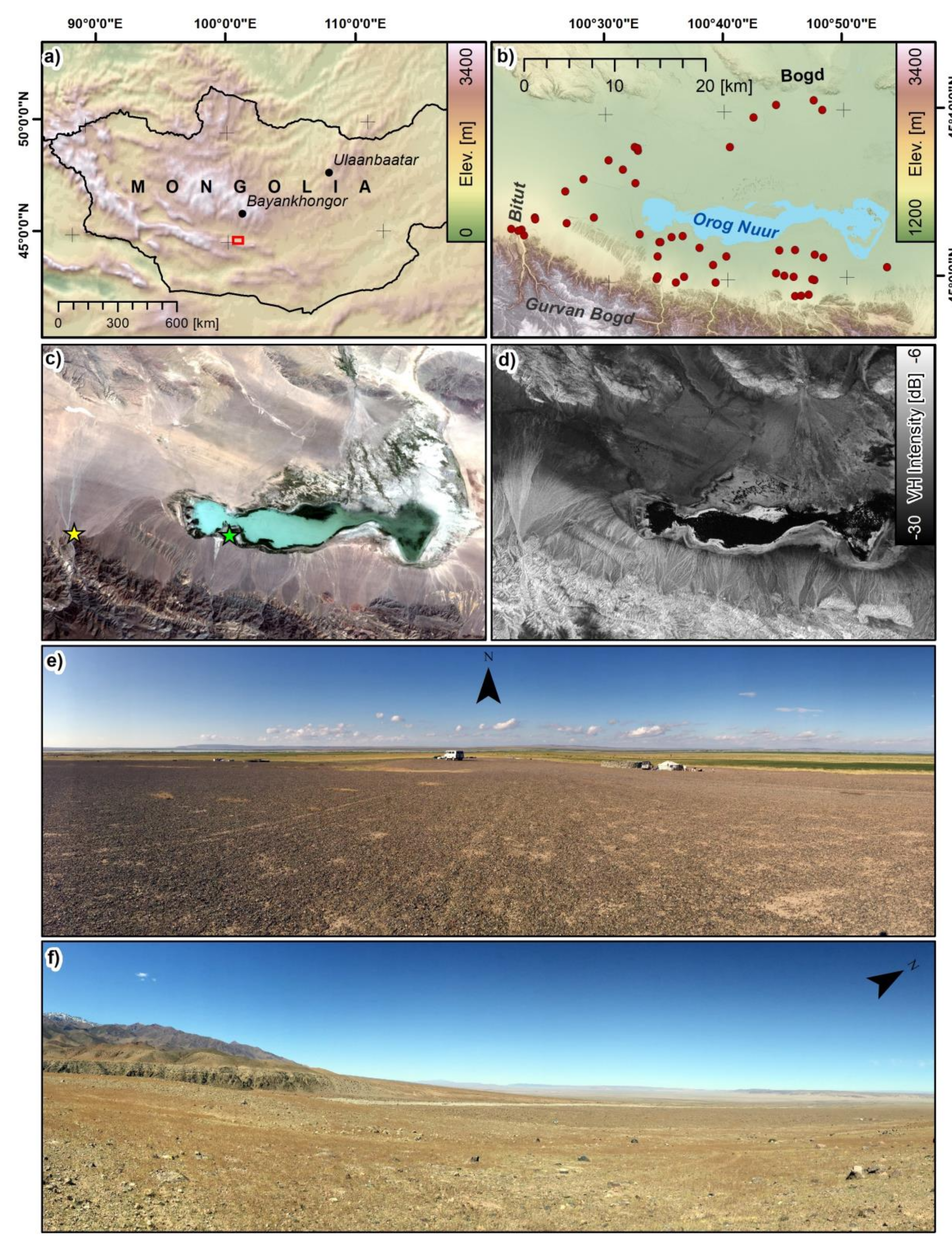
2.1. Study Area

The research was conducted around the lake Orog Nuur in the Valley of the Gobi Lakes in southern Mongolia. The Valley of the Gobi Lakes formed since the late Cenozoic [34,35]. Recent active tectonics result in earthquakes with a magnitude of up to M8.1. The last major earthquake occurred in 1957 and led to a vertical offset at the northern side of Gurvan Bogd of several meters [36,37]. The basin of the Orog Nuur is bound to the north by the Khangai and to the south by the Gobi Altai and the Gurvan Bogd. Lake Orog Nuur is at an elevation of 1168 m, while the Gurvan Bogd in the south reaches up to 3957 m. The central part of the Guvan Bogd consists of granites, metamorphic rocks, and basalts, while quaternary sediments fill the basin. The Orog Nuur has a size of roughly 140 km² and a depth of up to 3 m. However, considerable lake level variations occur in recent times as well as throughout the Holocene [38,39].

The main inflow of the lake is the Tuyn Gol river, which originates in the Khanghai Mountains and enters the basin of the Orog Nuur from the North (close to town of Bogd). A large variety of different types of surfaces occur in the basin of the Orog Nuur. The Tuyn Gol in the northern part of the basin deposited a major alluvial fan with a size of more than 200 km². In contrast, alluvial fans on the southern shore of the lake are much smaller but have steeper gradients. Several terrace generations indicate varying depositional and erosional conditions [39]. Close to the lake on the northern shore several active dune fields developed, and the main dune type are barchans.

The climate of the area is arid to semi-arid with annual precipitation values of around 100 mm in the basin and most likely higher values in mountain ranges [40]. The precipitation maximum is in June and August [39] under the influence of the mid-latitude westerlies. During wintertime, the area is influenced by the Siberian High with mean monthly temperatures of around −20 °C in the basin. In contrast, mean monthly temperatures in July are at 16 °C. Vegetation in the area is generally very sparse, or absent. It mainly occurs close to the lake or in the mountain valleys in sheltered positions. Close to the lake, dwarf bushes and reed-halophytes are the dominant communities [40].

2.2. Datasets

2.2.1. Sentinel-1

In this study, 68 acquisitions of Sentinel-1B were investigated. The datasets were downloaded as single-look-complex (SLC) products from the Sentinel data hub (scihub.copernicus.eu). The acquisitions were taken in descending orbit using the interferometric wide swath (IW) mode. All data provided intensities in VV and VH polarization. The set included scenes acquired between 23 January 2017 and 27 September 2019; one scene (10 September 2019) was taken during the period of fieldwork (6–17 September 2019).

The entire study area (Figure 1) lied in the second swath (IW2), having a mid-rage incidence angle of 39.4°. The IW2 datasets were processed using the Sentinel applications platform (SNAP) software (version 7.0.2), IDL 8.7.2, and ENVI 5.5. A processing chain developed in preliminary work [7,41,42] was used to processes the terrain-corrected gamma nought VV (GVV) and VH (GVH) intensities (following the approach of [43], which is approximated as “Terrain-Flattening” function in SNAP). The TanDEM-X DEM (Section 2.2.3) with a pixel spacing of 12 by 12 m was used for the calibration, the terrain flattening, and the range-doppler terrain correction. The SAR features were projected and resampled to a common grid (world geodetic system (WGS) 1984, Universal Transverse Mercator (UTM) Zone 47 North) using bilinear interpolation and a pixel spacing of 20 by 20 m.

Using this stack, the minimum, mean and maximum intensities in VV and VH were processed for the winter (December, January, February) and the summer (July, August, September) season. These metrics were derived in the temporal direction of the stack and were investigated as they might suppress the effect of soil moisture in SAR intensity, which is potential due to occasional precipitations or remnant of last time precipitation. Finally, 14 SAR features (

Table 1. List of investigated Sentinel-1 features.

Name	Description	Acquisition Date or Period
GVHsingle	Terrain-corrected gamma nought VH intensity	10 September 2019
GVVsingle	Terrain-corrected gamma nought VV intensity	10 September 2019
µGVHsummer	Mean terrain-corrected gamma nought VH intensity	July/August/September 2017–2019
µGVVsummer	Mean terrain-corrected gamma nought VV intensity	July/August/September 2017–2019
µGVHwinter	Mean terrain-corrected gamma nought VH intensity	December/January/February 2017–2019
µGVVwinterr	Mean terrain-corrected gamma nought VV intensity	December/January/February 2017–2019
minGVHsummer	Minimum terrain-corrected gamma nought VH intensity	July/August/September 2017–2019
minGVVsummer	Minimum terrain-corrected gamma nought VV intensity	July/August/September 2017–2019
minGVHwinter	Minimum terrain-corrected gamma nought VH intensity	December/January/February 2017–2019
minGVVwinterr	Minimum terrain-corrected gamma nought VV intensity	December/January/February 2017–2019
maxGVHsummer	Maximum terrain-corrected gamma nought VH intensity	July/August/September 2017–2019
maxGVVsummer	Maximum terrain-corrected gamma nought VV intensity	July/August/September 2017–2019
maxGVHwinter	Maximum terrain-corrected gamma nought VH intensity	December/January/February 2017–2019
maxGVVwinterr	Maximum terrain-corrected gamma nought VV intensity	December/January/February 2017–2019

) were compared with the surface roughness indices (Section 2.3), while the full time series of GVV and GVH were compared to the auxiliary data (Section 2.2.3).

The analyses involved two consecutive steps (described in Section 2.4). In the first step, the linear scaled intensities ($I_{linear}$) of the SAR features were investigated. In the second step, the intensities were converted to decibel (dB) ($I_{dB}$) using Equation (1):

$$I_{dB}=10lo{g}_{10}\left(I_{linear}\right).$$

(1)

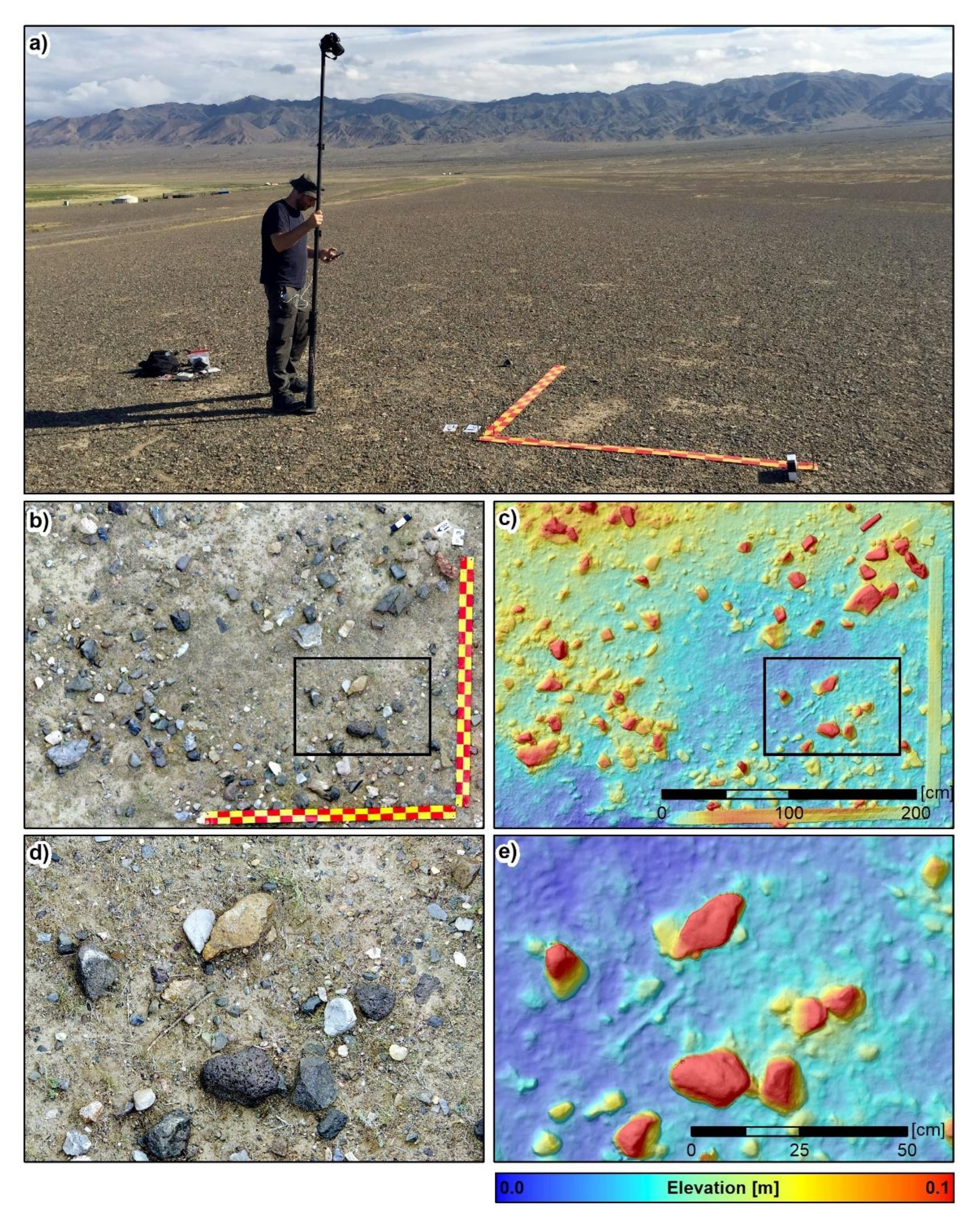
2.2.2. Fieldwork and Sampling

During the 6 September and 17 September, 2019, fieldwork was conducted in the Orog Nuur basin. Surface properties were documented for 48 plot locations (Figure 1). The plots were set up around the lake on sites that showed none to very sparsely vegetated ground. In the field, the plot locations were chosen based on expert judgment, so that they (i) represent different surface roughness types that are most typical for this region (e.g., alluvial fan surfaces, beach ridges, desert pavements, etc.), (ii) are placed in the center of a homogeneous area (covering at least 30 by 30 m) showing similar surface roughness properties over a larger distance, (iii) lie in open and gently sloped terrain (i.e., outside the mountain range), and (iv) have none or sparse vegetation coverage.

For each plot, the sites’ specifics were described and documented, and the location of the plot was recorded using a standard GPS device (Garmin GPSmap 60CSx). For all plots, the reported X/Y location error was less than +/- 5 m. The soil moisture of the upper soil profile was measured (see Section 2.2.3). A plot area of 2 by 2 m was marked using two 200 cm measuring tapes with a width of 10 cm. Further, a reference box with height of 9.7 cm was placed next to the measuring tapes, but outside the inner 2 by 2 m core area. During the following measurements, the tapes were secured to the ground using steel pins to avoid wind-induced movement. A standard camera (Pentax K-S2 with 20.1 mega pixels) was mounted on a pole (PHOTOMAST MK2), tilted towards the ground and elevated to 3.5 m height above ground. Using a focal length of 18 mm (which corresponds to 27 mm focal length due to the crop factor of the camera’s sensor), a shutter speed of <1/500 s and a maximum ISO of 400, images of the plot area were taken from various positions; however, avoiding shadows in the inner core area. The number of images ranged between 40 and 90 per plot. The acquisition setup is illustrated in Figure 2. These images were then used in photogrammetric processing to derive DEMs and ortho-mosaics. This was realized using the software Agisoft Photoscan 1.2.6 and following the standard processing workflow. In the first step, the images of one plot were aligned using high accuracy and generic pair selection.

The number of tie points ranged approximately between 15,000 and 30,000. In the second step, the dense point cloud was derived using high quality and aggressive depth filtering options. The number of points was on average 3E+7. The dense point cloud was then rotated to the true X, Y, and Z directions using markers that were manually placed on images showing the measuring tapes and assuming Z = 0 for all points (i.e., models then display the surface elevation relative to the plain defined by the two measuring tapes). In the third step, the DEM and the ortho-mosaic were processed with a pixel spacing of 0.2 cm, of 0.1 cm respectively, meeting the sampling interval for C-Band data (0.5 cm) recommended by [44].

Table 2. Accuracy of the ground-based DEMs displayed as absolute root mean square error (RMSE).

Dimension	RMSE (cm)	Number of Samples
X/Y	0.34	106
Z	0.90	96

reports the accuracies of the processed ground-based DEMs in X, Y, and Z direction.

The accuracies were estimated by comparing the known and estimated length and height of reference objects. The two 200 cm measuring tapes were used to assess the error in X and Y dimension, while the reference box was used to assess the absolute error in the Z dimension. The tapes and the box were placed inside the photographed area (i.e., they were therefore visible in the photogrammetric model), but outside the inner 2 by 2 m core area, for which the roughness indices were calculated in the later processing (Section 2.3 and Figure 3). The DEMs were of high precision and provided absolute root mean square errors (RMSE) of 0.34 cm in X/Y direction and 0.90 cm in Z direction. Thus, they were considered accurate enough to provide proxies on the surface roughness.

2.2.3. Auxiliary Data

Auxiliary datasets were used to judge on the quality of the reference data and the selected plot locations. Along with the ground-based photography, the soil moisture in the upper 7 cm of the soil profile was measured in September 2019 using a Delta-T WET-2 sensor. For each plot, several soil moisture measurements were conducted to ensure reliable estimates. It turned out that no single measurement exceeded a value of 7% soil moisture, but nearly all measurements (95%) showed soil moisture values less than 4%. Thus, all plots showed very dry conditions, at least during the period of fieldwork.

Further, the terrain slope was estimated for each plot location using the TanDEM-X DEM in order to account for potential macro topographic effects (i.e., these might reveal in the later analyses as this DEM was also used in the processing of the Sentinel-1 data). The DEM was provided by the German Aerospace Center (DLR) via a science proposal (see Acknowledgments). The DEM had a pixel spacing of 12 m by 12 m after projecting it to the coordinate system of the Sentinel-1 data. For the plot locations, the maximum slope was 5.2°, while the average slope was 2.3°. Thus, all plots were situated in gently sloped terrain.

To get insights on the past (2017–2019) land surface properties and precipitation events, we have investigated freely available time series of archive data, which are listed and described as follows. The main purpose of these datasets is to characterize the temporal dynamics of the site (i.e., analyzing the temporal behavior of properties that might affect the SAR signal, such as vegetation, land surface temperature, soil moisture, and precipitation). These datasets are further used to investigate the sensitivity of the SAR signal to changing surface conditions. The used auxiliary datasets were:

Precipitation: Information on past precipitation events (2017–2019) were collected from the observations of the global precipitation measurement (GPM) mission (gpm.nasa.gov). The used product (IMERG Final Run) shows the daily accumulated precipitation in mm at a spatial resolution of approximately 5 by 15 km.

Vegetation: The time series (2017–2019) of the MODIS product MOD13A1.006, which shows the normalized difference vegetation index (NDVI) aggregated at 16-day intervals and at a spatial resolution of 500 by 500 m, was accessed using the cloud-based processing service AppEEARS (Application for Extracting and Exploring Analysis Ready Samples; lpdaac.usgs.gov). In addition, results were compared to Landsat datasets acquired during the summer months (July, August, and September) in 2017, 2018, and 2019. Landsat data was processed in the Google Earth Engine [45] using a script developed in preliminary work [46].

Land surface temperature: Similar, the MODIS time series (2017–2019) of the product MYD11A2.006 was accessed using the AppEEARS service. It shows the average daily day and night land surface temperature (converted to °C) at a spatial resolution of 1 by 1 km.

Soil moisture: Information on soil moisture estimates were taken from the ERA5-Land reanalysis datasets provided by the European Centre for Medium-Range Weather Forecasts (ECMWF; ecmwf.int). The variable “Volumetric soil water layer 1” was investigated as it shows model results on the average daily soil moisture in m³/m³ for the upper 0 to 7 cm of the soil profile. The data had a spatial resolution of 8 by 10 km.

2.3. Surface Roughness Indices

From the ground-based DEMs several surface roughness indices (

Table 3. List of investigated surface roughness indices.

Name	Description	Direction	Estimation	Unit
RMSH profile	Root Mean Square Height	Vertical	X/Y Profiles	(m)
RMSH circular			Circular Profiles
RMSH 2D			Surface
CORL profile	Correlation Length	Horizontal	X/Y Profiles	(m)
CORL circular			Circular Profiles
CORL 2D			Surface
ZVAL profile	Z-Value	Vertical and horizontal	X/Y Profiles	-
ZVAL circular			Circular Profiles
ZVAL 2D			Surface
TORT profile	Tortuosity Index	Vertical and horizontal	X/Y Profiles	-
TORT circular			Circular Profiles
TORT 2D			Surface

) were calculated. Each index was estimated using the 2 by 2 m subset of the DEM and all processing steps were carried out in IDL 8.7.2. The DEMs were de-trended prior to the index estimation to remove effects caused by the overall terrain slope. The fit to the DEM surface was realized using the IDL function SFIT with a maximum degree of three for the fitting polynomial. As pointed out by [47] the detrending removes higher order effects of the macro-topography and is crucial to make the surface roughness estimates independent of the overall terrain slope. The detrending is most important for features accounting for the horizontal roughness variations and higher polynomial degrees might even be needed for sites with complex topographic settings [47]. We decided to stay with the same, rather low polynomial order for all plots, as sites were situated in a rather gentle sloped (natural) terrain. Further, a maximum degree of three for the fitting polynomial turned out to be sufficient in the later variogram analysis.

The roughness indices were estimated in three different ways using the DEMs: (i) First, indices were estimated from virtual profile lines that were placed along each row and each line of the fitted DEM. The DEMs had a pixel spacing of 0.2 cm and therefore 2000 profile lines were processed (1000 in X-direction and 1000 in Y-direction). From these 2000 measurements, the median roughness index value was estimated. In a pre-test, the lowest (minimum) and highest (maximum) index values were returned, but their correlation to the SAR intensities was always lower than the correlation obtained from the median, these correlations were also mostly not significant (p-value > 0.01, see Section 2.4). Therefore, in the further analyses, just the median values were considered. (ii) Second, the surface roughness indices were estimated using virtual profiles of 2 m length, centered on the midpoint of the inner 2 by 2 m core area. The median index value was then estimated from 180 profiles that were consecutively rotated by steps of 1° around the midpoint (i.e., the surface roughness estimation is then based on measurements in each azimuth direction). (iii) Third, indices were directly estimated from the digital representation of the surface in a two-dimensional (2D) space. The surface roughness indices considered in the analyses are described in the following.

Root mean square height (RMSH): The RMSH is the standard deviation (Equation (2)), where n is the number of the samples, $z\left(x_i\right)$ the height value at position $x_i$ and $\overline{z}$ the mean height. RMSH accounts for the vertical elevation changes and higher index values indicate higher surface roughness [19]. RMSH was calculated along the X/Y profiles, the circular profiles and for the samples of the variogram (see below).

$$RMSH=\sqrt{\frac{1}{n}{{\displaystyle \sum }}_{i=1}^n{\left(z\left(x_i\right)-\overline{z}\right)}^2}.$$

(2)

Correlation length (CORL): The CORL is calculated for the X/Y profiles and the circular profiles via the autocorrelation function (ACF) (Equation (3)). ACF calculates the correlation between two samples as a function of their spacing, the horizontal distance between both samples, respectively. In Equation (3), 〈〉 is the averaging, $z\left(x_i+\delta \right)$ is the profile elevation at position $x_i$ plus the lag distance $\delta$, and $z\left(x_i\right)$ the profile elevation at position $x_i$. ACF is normalized via the squared RMSH. The functions ranges from −1 to +1. ACF was processed in IDL using the A_CORRELATE function. The CORL is the value at which the ACF drops the $e^{-1}$ criteria (i.e., the lag distance at which two elevation values become statistically independent). In Equation (4), e is the mathematical constant Euler’s number. Lower values of CORL indicate higher horizontal variations of the surface [21,30].

$$ACF\left(\delta \right)=\frac{〈z\left(x_i+\delta \right)z\left(x_i\right)〉}{RMS{H}^2},$$

(3)

$$CORL=AC{F}^{-1}\left(e^{-1}\right).$$

(4)

CORL can be estimated directly from 2D surfaces (e.g., DEMs) by conducting a (semi-)variogram analysis [23,47]. The empirical (semi)-variogram ($\widehat{\gamma }$) is calculated for a sample (here 50,000 points) and an exponential model is fitted, representing the theoretical variogram ($\tilde{\gamma }$). The ACF can be calculated from $\tilde{\gamma }$ (Equation (6)), where $\tilde{\gamma }\left(\infty \right)$ is the value of $\tilde{\gamma }$ at 95% of the sill of the fitted exponential model and $\tilde{\gamma }\left(\delta \right)$ is the semi-variance at lag distance $\delta$ [47].

$$\widehat{\gamma }\left(\delta \right)=\frac{1}{2n}{{\displaystyle \sum }}_{i=1}^n{\left(z\left(x_i\right)-z\left(x_i+\delta \right)\right)}^2,$$

(5)

$$ACF\left(\delta \right)=1-\frac{\tilde{\gamma }\left(\delta \right)}{\tilde{\gamma }\left(\infty \right)}$$

(6)

The (semi)-variogram was processed in IDL using the VARIOGRAM function provided by J. Mc Creight (University of Colorado). The fitting of the exponential model was realized using the COMFIT function and the GOMPERTZ option. The fit between the exponential models and the empirical variograms was very high with r² values ranging from 0.81 to 0.99. Therefore, we consider an exponential model as appropriate, which is in accordance to results from other studies (e.g., [21]).

Z value (ZVAL): The ZVAL relates the RMSH and CORL by the ratio shown in Equation (7). The intention of this parameter is to account for vertical and horizontal variations in a single index [30]. Higher values of ZVAL are indicative for higher surface roughness.

$$ZVAL=\frac{RMSH}{CORL}.$$

(7)

Tortuosity index (TORT): For the X/Y profiles and the circular profiles TORT is defined by the ratio between the true length ($L$) of a profile and its projected horizontal length ($L_0$) (Equation (8)). Therefore, TORT accounts for vertical and horizontal variations along the profile. Here TORT was shifted to a minimum value of 0, while originally TORT has a minimum 1. TORT is increasing with increasing roughness [30].

$$TORT=\frac{L}{L_0}-1.$$

(8)

TORT can be estimated directly from the DEM by estimating the true area ($A$) of the surface and its projected horizontal area ($A_0$) (Equation (9)). Both areas were estimated in IDL using the function MESH_OBJ and MESH_SURFACEAREA. Again, TORT was shifted to a minimum value of 0

$$TOR{T}_{2D}=\frac{A}{A_0}-1.$$

(9)

2.4. Referencing and Inversion

A regression modelling was applied in order to investigate the capacity of the SAR variables (Table 1) to predict the surface roughness indices (Table 3) and to investigate the relation/correlation among the surface roughness indices and the Sentinel-1 features themselves. In the regression modelling, the paired independent (x) and dependent (y) variables are fitted to a user-supplied function by minimizing the error statistic. The model returns the fitted model parameters ($a_1, a_2, \dots a_n$) and the calculated/estimated function values ($\widehat{y}$). The number of the model parameters depends on the investigated model.

Here, two functions were investigated, which were a simple linear model (Equation (10)) and simple exponential model (Equation (11)). Both models are described by two model parameters ($a_1, a_2$). The modelling was performed in the IDL using the functions REGRESS, and CURVEFIT.

$$\widehat{y}=a_{1}x+a_2,$$

(10)

$$\widehat{y}=a_1{e}^{a_{2}x}.$$

(11)

The linear model was used whenever the surface roughness indices and/or the linear-scaled Sentinel-1 intensity features were analyzed. The exponential model was used whenever the surface roughness indices and the logarithmic-scaled Sentinel-1 features (i.e., showing intensities in decibels (Equation (1)) were used. This was done to account for the expected saturation of SAR intensity values with increasing surface roughness (see Section 2.2.1) and to account for the logarithmic scaling. The exponential model was further used to fit the semi-variogram for the estimation of the 2D autocorrelation length.

For all models, the Pearson Correlation Coefficient (r) was estimated. This coefficient is defined by the ratio of the covariance and the product of the individual standard deviations of two variables (Equation (12)). It was processed in IDL using the CORRELATE function. The coefficient quantifies the degree of determination between the two variables on observation and it ranges from −1 to +1, where an absolute value of one indicates perfect correlation and maximum determination, whereas a value of zero indicates no correlation and minimum determination [25]. Along with r, the p-value was processed using a two-sided t-test. The p-value was estimated using the IDL function LINCORR, provided by Simon Vaughan (University of Leicester). A correlation was assumed statistically significant if its corresponding p-value was below a value of 0.05. The importance of the p-value to judge whether a correlation is significant or not highly depends on the sample size and larger sample sizes inherently cause lower p-values [48]. However, as our sample size was rather small (n = 48) we consider the estimated p-values to be reliable and meaningful.

$$r=\frac{{{\displaystyle \sum }}_{i=1}^n\left(y_i-\overline{y}\right)\left({\widehat{y}}_i-\overline{\widehat{y}}\right)}{\sqrt{{{\displaystyle \sum }}_{i=1}^n{\left(y_i-\overline{y}\right)}^{2^{}}}\sqrt{{{\displaystyle \sum }}_{i=1}^n{\left({\widehat{y}}_i-\overline{\widehat{y}}\right)}^2}}.$$

(12)

Additionally, the root mean square error (RMSE) was used to quantify the precision of the models. RMSE is a measure for the deviation between the observed and predicted values (Equation (13)). In the equation, $\widehat{y_i}$ denotes the predicted values, $y_i$ denotes the observed values, and $n$ denotes the number of samples. RMSE is expressed in the same unit as the input variables. Along with this, the unbiased RMSE (ubRMSE) was processed as well [49,50].

$$RMSE=\sqrt[]{{{\displaystyle \sum }}_{i=1}^n\frac{{\left(\widehat{y_i}-y_i\right)}^2}{n}}.$$

(13)

The analyses finally involved two consecutive steps: (i) In the first step, the correlations among the surface roughness indices and the linear-scaled Sentinel-1 intensity features were analyzed. This was done assuming a linear model (Equation (10)) and using all available plots (n = 48). The result of this assessment was used to indicate the variables that were significantly correlated, while surface roughness indices showing very low correlation with the SAR features, or no significance, were omitted from the following analyses. (ii) In the second step, the relations between selected surface roughness indices (the ones indicated in the first step) and the logarithmic-scaled Sentinel-1 features were estimated. Therefore, this analysis aimed to indicate the best and most significant exponential models (Equation (11)) that allow inverting Sentinel-1 intensities to surface roughness indices. This was realized by splitting the reference data of all available plots (n = 48) into two sets that were used for training (n = 24) and validation (n = 24). Therefore, a training set was used to estimate the parameters of the exponential model ($a_1, a_2$), while the corresponding validation set was used to independently estimate the model quality (r, p-value, RMSE).

However, using this technique the quality of the model was dependent on the split in training and validation. A common way to overcome this limitation is the k-fold-cross validation (e.g., [51]), or the leave one out technique (e.g., [52]). As our sample size was rather small (n = 48), we doubt that these approaches ensure reliable estimates. Instead, a multi-model approach with 2000 iterations was applied. The split in training and validation sets was done randomly 2000 times for each variable pair under observation (one Sentinel-1 feature and one surface roughness index). During each iteration, the CURVEFIT function was applied to estimate the best fitting function parameters of the exponential model ($a_1, a_2$). The quality of the model was then reported. After the loop, the statistics (minimum, lower quartile (25%), median, upper quartile (75%), and maximum) of the r, p-value and RMSE values were calculated. This processing was repeated for all possible combinations of variable pairs (i.e., all Sentinel-1 features were tested against all selected surface roughness indices). To its end, this technique allows quantifying the model quality and the deviation of the estimated model parameters. Robust and significant relations between surface roughness indices and SAR intensities are revealed by high r, low RMSE, p-value < 0.01 and similar exponential models. Further, this technique allows finding the model function that shows the best trade-off between over- and under-estimation by selecting the model that best fits the median of all predicted values from all investigated models. This function inverts the SAR intensity; as well, the multi-model approach allows indicating the expected deviation (i.e., confidence interval). This deviation in turn specifies the inherent uncertainty that arise in the empirical modelling from the split of the samples in training and referencing and it can be drawn in the map-space along with the inversion results.

3. Results

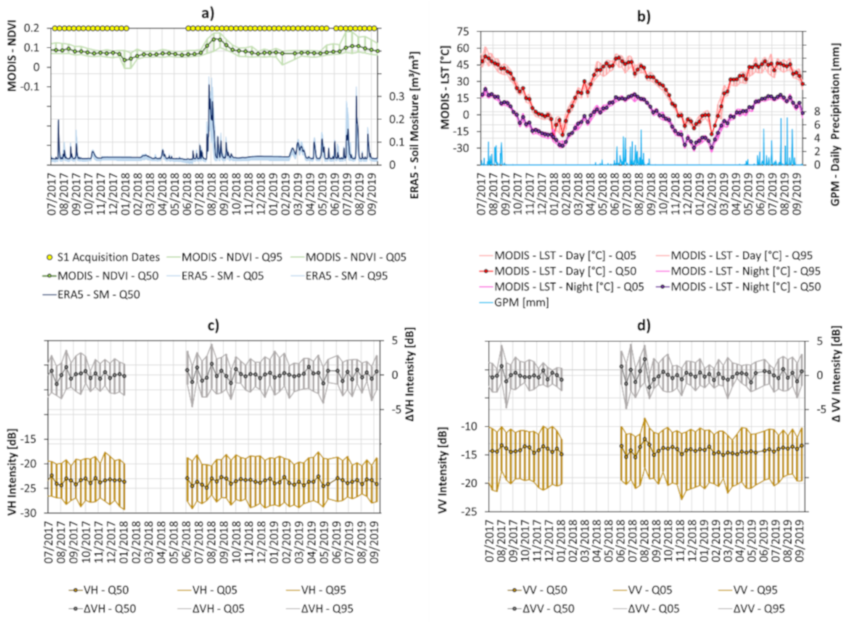
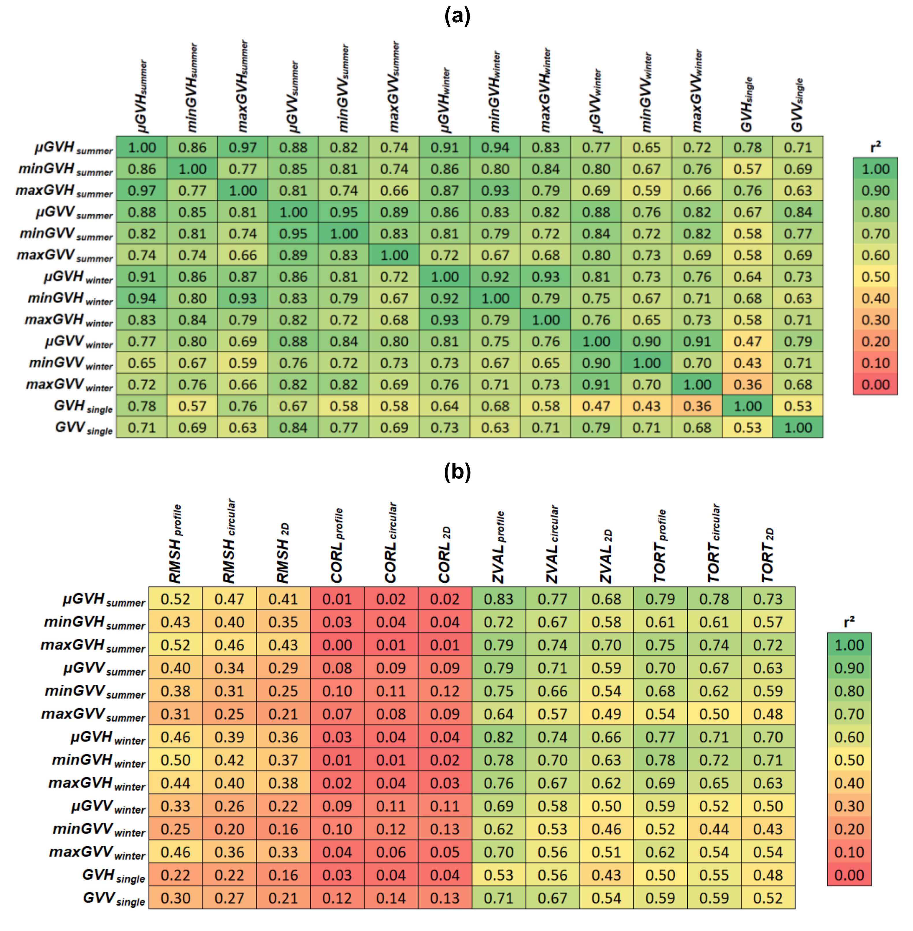
3.1. Relation of SAR Features and Auxilary Data

The initial analyses compare the time series of Sentinel-1 features and the auxiliary datasets. Figure 3 draws the features values between 1 July 2017, and 30 September, 2019, for plots located in >10 km distance to the lake (n = 23). The selection of the plots is done to avoid effects resulting from the coarse spatial resolution of ERA5 data and to cancel out pixels influenced by the lake and its surrounding vegetation. NDVI series (Figure 3a) between 2017 and 2019 shows that NDVI is generally very low over the plot locations (0.09 on average).

However, distinct phases of vegetation greening are observable over some of the plots in summer 2018 (between August 2018 to September 2018) and in summer 2019 (between June 2019 to September 2019), reaching NDVI values up to a maximum of 0.2. ERA 5 soil moisture data show distinct peaks up to 0.33, occurring in good accordance with temporal peaks of NDVI and precipitation (Figure 3b). Further, ERA5 data indicate very low soil moisture conditions (<0.05) for most parts of the year and for the period of fieldwork (6 to 17 September, 2019), which matches the in situ measurements (Section 2.2.3). Potential freeze of the surface, indicated by MODIS LST observations (Figure 3b), is most likely due between end of October (first observations with LST < 0°C during the night time) to the end of April (last observations with LST < 0°C during the night time). The VV and VH intensities (Figure 3c,d) are very stable over time and median intensity is around −23 dB (VH) and −14 (VV) for all seasons. The temporal variations over the plots locations, expressed by differencing the intensity values of consecutive acquisitions (∆VH and ∆VV), show, for the most part, small alterations < +/− 2 dB and a median of around 0 dB; however, a clear increase of VH and, especially, of VV intensities is observable in summer 2018, matching the period of increased NDVI values. Similar, VV intensities tend to increase gradually between early June 2019 and early September 2019 (best visible for ∆VV in Figure 3d), which corresponds to the period of increased NDVI values detected by MODIS. Interestingly, the VH intensities seem to be insensitive to this greening event, as median values are stable and variations (∆VH) do not show noticeable variations, but are of low magnitude for the respective period (early June to end of August 2019).

In summary, the analyses of the auxiliary and Sentinel-1 time series indicated that: (i) prior to the field work (June to August 2019) there was a phase of increased precipitation that likely led to increased soil moisture, as indicated by the ERA5 reanalysis data. During this phase, NDVI of MODIS increased and showed a NDVI peak up to 0.2. (ii) For the period of field work (September 2019) the NDVI values had already decreased to NDVI values < 0.09, while ERA5 data indicate very dry conditions of the upper 7 cm of the soil profile (soil moisture < 0.05). This matches the in-situ observations on the state of the vegetation (none to very sparse coverage) and the soil moisture measurements (soil moisture < 0.05). (iii) The SAR signal over the plots is very stable in time and no seasonal differences are distinguishable. Freeze and thaw cycles seem not to affect the VV/VH intensities. (iv) Some single events (potentially of high magnitude) affect the SAR signal, e.g., VV intensities show increased values in parallel to the increased NDVI values in summer 2019, while VH intensities seem to be insensitive to this event.

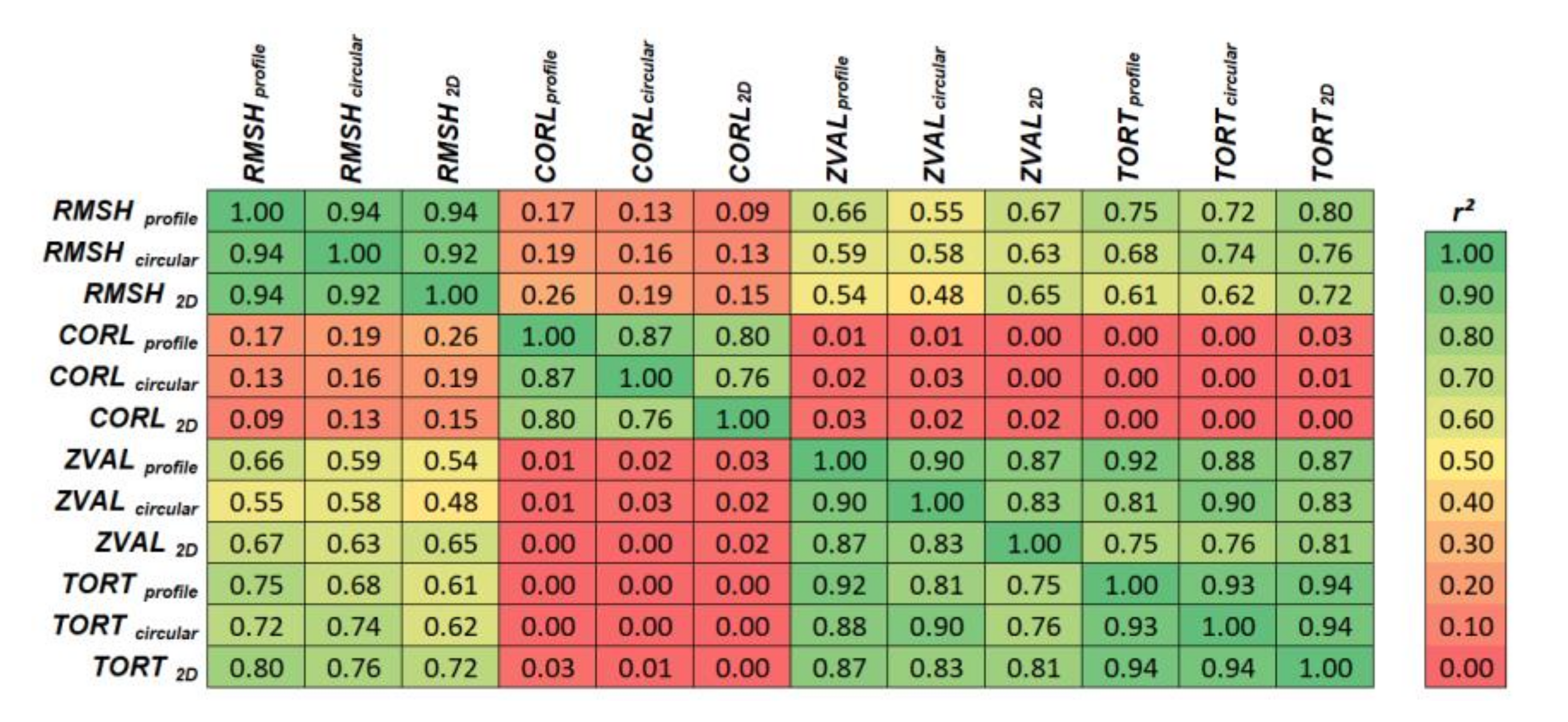
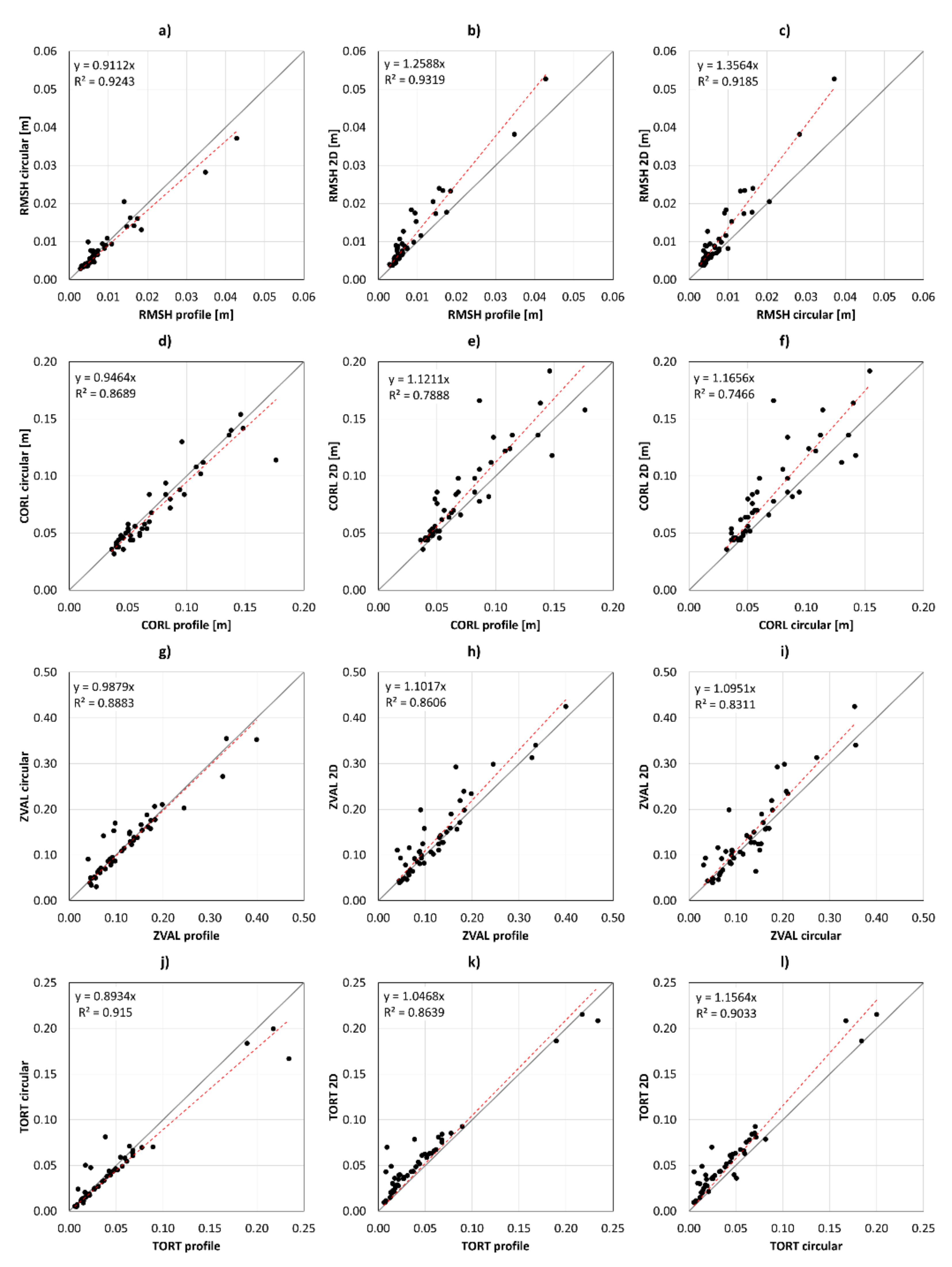
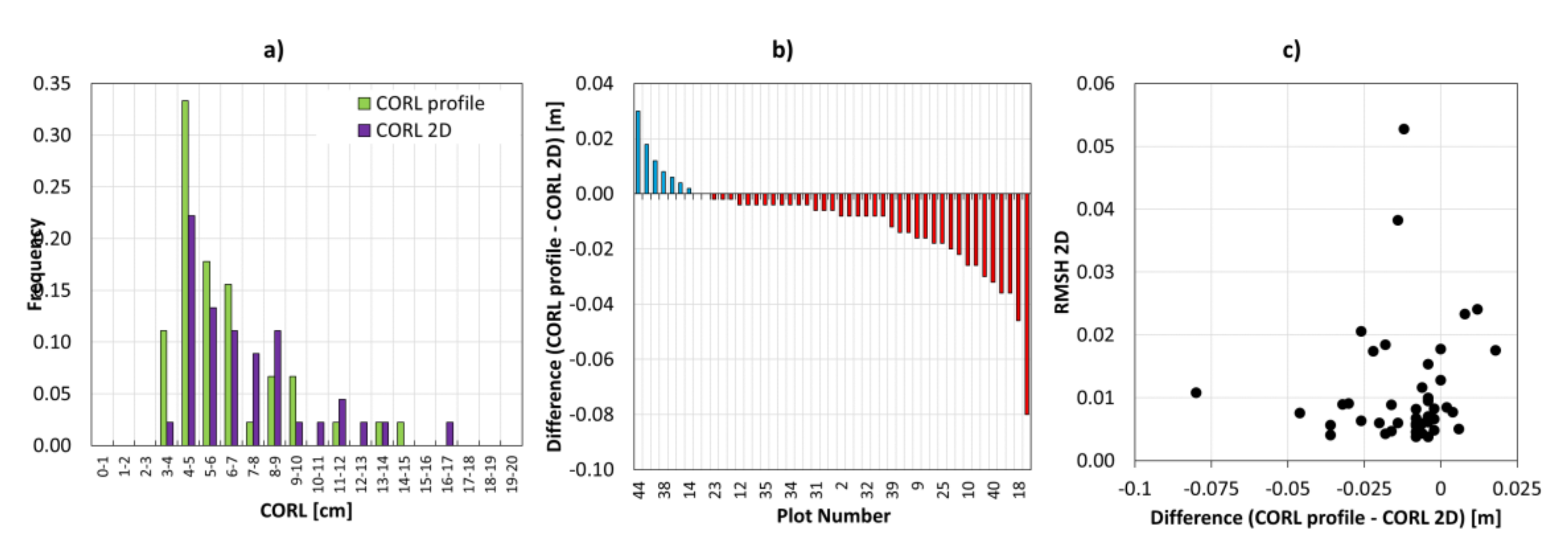
3.2. Relation of 1D and 2D Surface Roughness Indices

The 1D and 2D surface roughness indices were analyzed prior to the multi-model assessment, as the different approaches might cause different surface roughness estimates. Figure 4 and Figure 5 indicate the relation between the 1D (profile, circular) and 2D surface roughness indices (Table 3) using data from all plots (n = 48). It turned out that RMSH estimates of all approaches are very similar (Figure 5a–c) and r² values are around 0.92. Similar, the 1D and 2D estimates of ZVAL and TORT are highly correlated with a minimum r² of 0.83 (Figure 5g–l). Further, all CORL values are positively correlated (Figure 5d–f) and the correlation is highest for the CORL_circular and CORL_profile (r² of 0.87). CORL_2D is best correlated with CORL_profile (r² of 0.80). However, it is observed that the 2D estimates of CORL are biased and the 2D approach is indicating longer CORL values (Figure 6a,b). As this is pointing to a potential systematic error, the difference between CORL_profile and CORL_2D is compared to RMSH_2D, but no relation was found (Figure 6c).

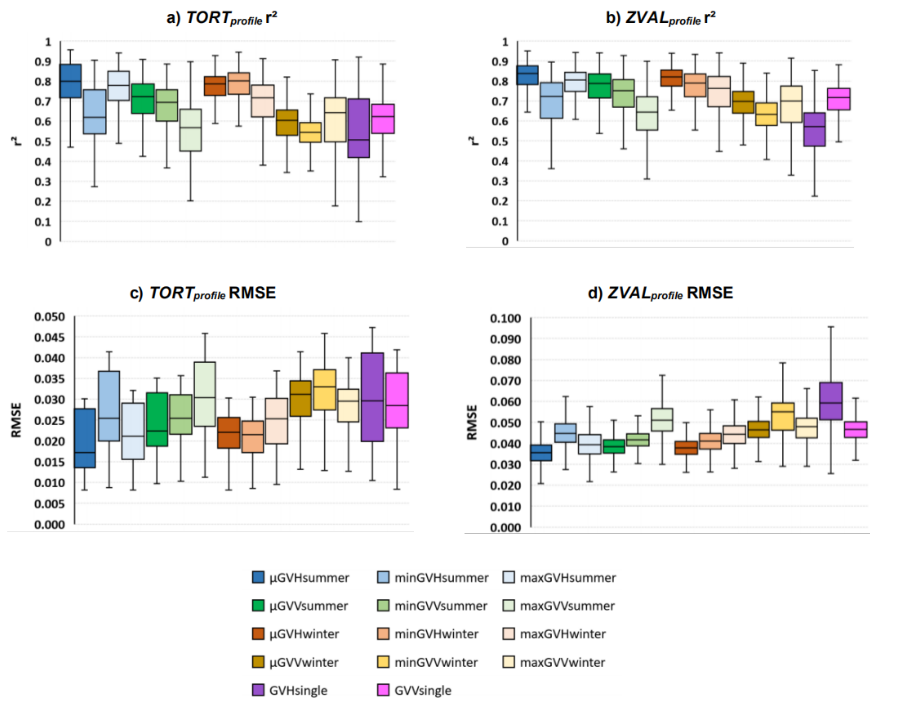
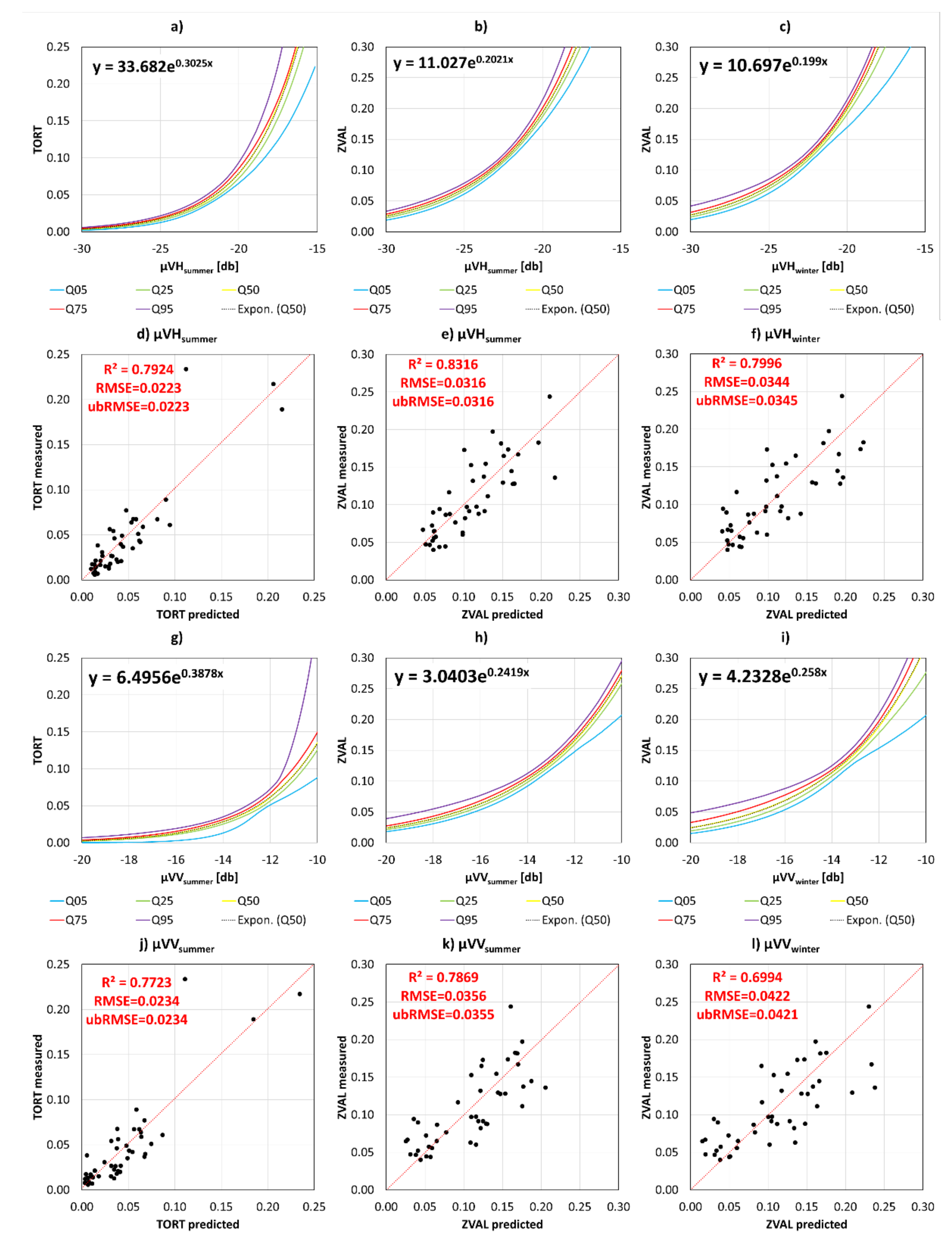
3.3. Relation of Surface Roughness Indices and SAR Intensities

Figure 7a draws the correlations among the investigated SAR features (Table 1) over the plot locations (n = 48). The results support the findings of the time series analysis (Figure 3) and correlations are high for almost all features. The missing seasonality of the SAR signal reveals high correlations of winter and summer features, e.g., r² of µGVH_summer and µGVH_winter is 0.91.

As well, the VV and VH intensities being highly correlated, e.g., r² of µGVH_summer and µGVV_summer is 0.88. Lowest correlations are found, when comparing minimum and maximum intensities of the multi-temporal features (minimum r² of 0.59 for minGVV_winter and maxGVH_summer). The intensities of the single scene (10 September, 2019) are highly correlated with the respective summer averages, e.g., r² of 0.78 for GVH_single and µGVH_summer, and r² of 0.84 for GVV_single and µGVV_summer.

Analyzing the relation between the SAR features and the surface roughness indices (Figure 7b), is observed when none of the CORL estimates are directly correlated with the SAR features (r² < 0.13, p-value > 0.05). Further, RMSH indices are only weakly correlated and best correlation is found for µGVH_summer (r² of 0.52, p-value < 0.05). Contrary, the indices TORT and ZVAL, which are sensitive to the horizontal and vertical variations of the surface, show higher r² values; for example, r² of 0.83 for µGVH_summer and ZVAL_profile and r² of 0.79 for µGVH_summer and TORT_profile. Again it is observed that differences due to the seasonality (summer/winter) are of minor relevance, e.g., r² is 0.82 for µGVH_winter and ZVAL_profile and therefore on the same level as the correlation of ZVAL_profile with µGVH_summer (r² of 0.83, as indicated above). The comparison reveals that correlation between a SAR feature and a surface roughness index is in all cases highest for the 1D estimate (Figure 7b). In most cases, the approach using the X/Y profiles to estimate the surface roughness index from the DEM yields the highest correlations with the SAR features, followed by the circular method, and the 2D approach.

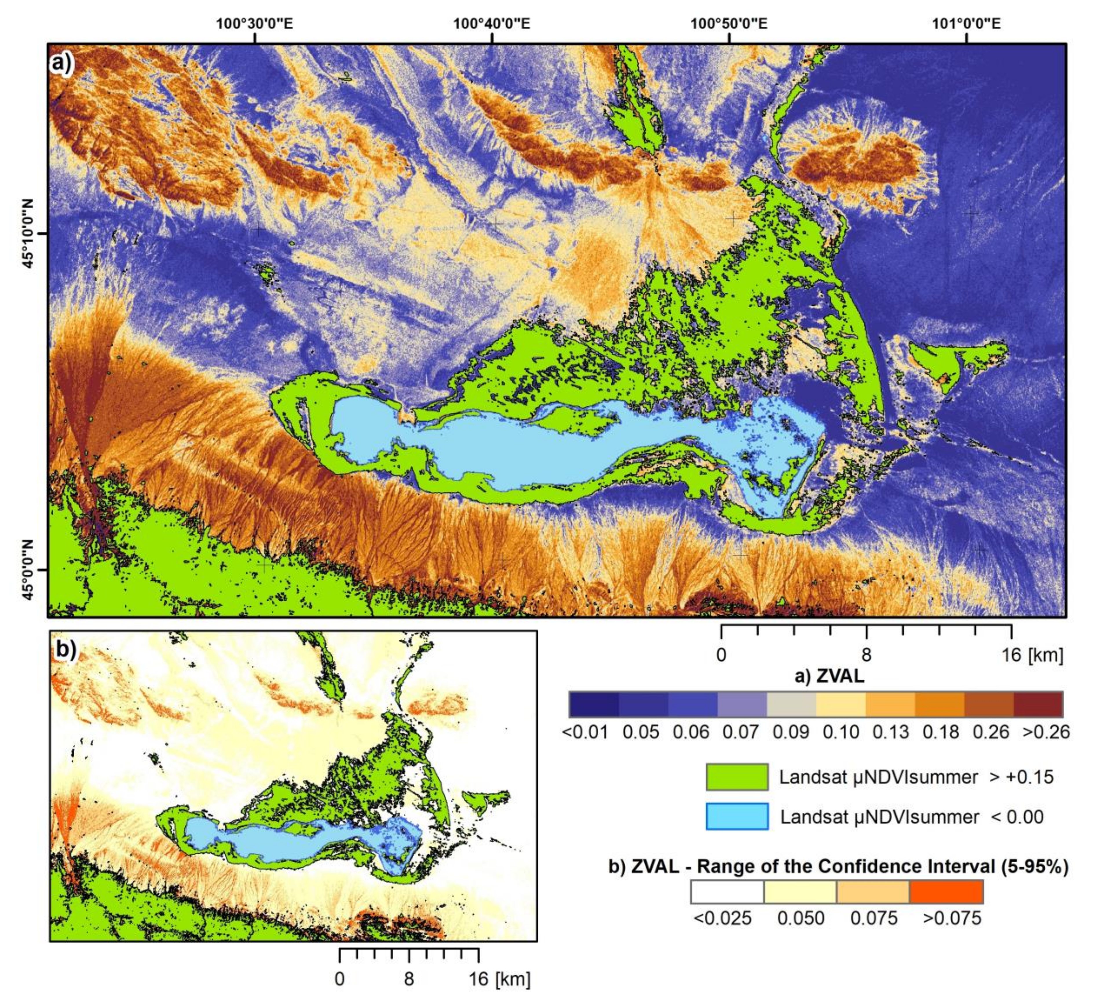
3.4. Referencing and Inversion

These results are further evaluated for ZVAL_profile and TORT_profile, which are the two roughness indices that showed the best correlation with the SAR features, by applying the multi-model assessment (specified in Section 2.4). Boxplots on resulting r² and RMSE are presented in Figure 8 for all SAR features, based on 2000 iterations.

In summary: (i) best relation between Sentinel-1 features and TORT/ZVAL is found for µGVH_summer and µGVH_winter, (ii) the mean intensity of a season is higher correlated with TORT/ZVAL than the corresponding minimum or maximum intensity of the same season, (iii) VH features are on average higher correlated with ZVAL/TORT than the respective VV features, (iv) the seasonal mean intensities of summer (µGVH_summer and µGVV_summer) and winter (µGVH_winter and µGVV_winter) provide higher correlations with ZVAL/TORT than the respective single scene intensities (GVH_single and GVV_single), (v) this systematic is also observed for the RMSE and higher r² values infer lower RMSE values (Figure 9c–d), on average.

Based on these results, the statistics on the inversion functions, which were used to generate the results drawn in Figure 8, are presented in Figure 9 for TORT and ZVAL and for the SAR features µGVH_summer, µGVV_summer, µGVH_winter and µGVV_winter. Panels (a-c) and (g-i) show selected percentiles (i.e., 5% (Q05), 25% (Q25), 50% (Q50), 75% (Q75), and 95% (Q95)) of the predicted function values of the exponential models. Therefore, the colored lines do not show single functions, but the statistics on all model outputs. The results are drawn for typical ranges of SAR intensities, (i.e., −30 to −15 dB for VH and −20 to −10 dB for VV) and surface roughness index values (i.e., 0.0 to 0.3 for ZVAL and 0.0 to 0.25 for TORT). Each panel in (a-c) and (g-i) shows one single exponential function with a dashed black line. This function best fits the 50% percentile (Q50) and its equation is denoted in the upper-left corner of the panel. Panels (d–f) and (j–l) draw the scatterplots of the ZVAL/TORT values predicted using these functions (x-axis) and the measured surface roughness values (y-axis), along with the 1:1 line and the resulting r², RMSE and ubRMSE values.

In summary, the following main findings are made: (i) models using the VH intensity showed a smaller spread of the predicted surface roughness values than models using the VV intensity, this is especially true for ZVAL > 0.15 and TORT > 0.10 (i.e., uncertainty of the estimates increases with the intensity, the surface roughness value, respectively). (ii) Inversion functions of summer and winter are very similar, while the spread of the functions is larger for the winter features. This leads to higher correlations of the summer features with the measured surface roughness indices, compared to the winter features. (iii) For all plots it is observed that inversion functions of ZVAL predict more similar values than inversion functions of TORT (i.e., spread between the 5% and 95% percentiles is larger for TORT compared to ZVAL). (iv) The best inversions are found for ZVAL and µGVH_summer (r² of 0.83), ZVAL and µGVH_winter (r² of 0.799), TORT and µGVH_summer (r² of 0.792), and ZVAL and µGVV_summer (r² of 0.787).

The final surface roughness estimation is therefore processed for ZVAL and µGVH_summer using the inversion function of Q50 (Figure 9e). Results are drawn in Figure 10a along with the range of confidence interval (Figure 10b), which is estimated as the difference between Q95 and Q05 (Figure 9). The inversion results are overlaid by a NDVI classification processed using the Landsat datasets. The mask indicates pixels with µNDVI < 0.0 and µNDVI > +0.15, limiting the inversion results to sites where radar intensities are likely not controlled by vegetation and/or water (cf. [53,54]). Highest ZVAL values are observed over the alluvial fans system at the northern slope of the Gurvan Bogd, while aeolian sediments in the west and east of the lake Orog Nuur are characterized by low ZVAL values, despite the elevated desert pavements and fossil beach ridges (located northwest of the lake) that are revealed by higher ZVAL values. Results further indicate decreasing ZVAL values towards the foot slopes of almost all alluvial fans of the Gurvan Bogd system. For some fans, a clear separation of different surfaces/aprons is visible, e.g., the Bitut fan shows at least three systems with different surface roughness properties.

4. Discussion

4.1. Estimation of Surface Roughness via Ground-Based Photogrammetry and Relation of 1D and 2D Surface Rougness Indices

Ground-based photogrammetry allows for a quick and reliable sampling of the micro-topography of selected small areas. The DEMs used in this research were of high quality having a pixel spacing of 2 mm and a RMSE < 0.4 cm in X/Y direction and RMSE < 0.9 cm in Z direction, which compares well with related studies that used similar sampling techniques (e.g., [21,30,47]), but also with accuracies achievable by manual pin profilers [20]. Thereby, more comprehensive referencing using several ground control points (e.g., as shown by [21,47]) will further enhance the accuracy of the DEMs on the expanse of more time needed to collect the data. The horizontal resolution of the used DEMs fulfills the sampling distance suggested by [55] (0.2 times the average correlation length), which is 5 mm considering the average correlation length of 0.1 m (calculated for all 48 plots).

In this study, the number of images per plot ranged between 40 and 90, which was sufficient to construct DEMs of 2 by 2 m. Similar number of images were for example used by [30], which used 30 and 78 images per plot to generate DEMs. Generally, more images from more different positions should be taken if the topographic setting is rather complex. The length of the (virtual) profiles was 2 m, which compares well with related studies (e.g., [16,27,29] used profiles of 0.9 to 1.0 m lengths), but does not fulfill the criteria’s raised by [56] (further discussed by [20]), which suggest profile lengths of 4 to 20 m (i.e., 40 to 200 times the expected correlation length), which is, in the field, difficult to realize.

The locations of the plot area were chosen so that they best represent the local terrain and roughness properties. The plots were placed in the homogeneous areas (covering at least 30 by 30 m) showing similar surface roughness properties over a larger distance (e.g., selected aprons of alluvial fans, desert pavements). Therefore, we consider the plot locations to be representative, which is crucial as the 2 × 2 m plots are compared to the 20 × 20 m Sentinel-1 pixels. Considering the ongoing discussion on how surface roughness should be estimated [20] and the mismatch between the size of the ground-based DEMs and the investigated Sentinel-1 pixels, future work will target approaches that offer a larger coverage of high-resolution DEMs, e.g., potentially by using low-altitude drone acquisitions. This would allow increasing the profile lengths, the sample size and therefore the reliability of the estimates. This will also support the analysis of sites that are more variable and where small ground-based DEMs cannot capture the full complexity of the terrain and its roughness.

The indices considered in this study were widely used in related work to quantify surface roughness (e.g., [16,28,29]) and they were estimated in three different ways: 1D along X/Y profiles, 1D along circular profiles and 2D using a variogram analysis. The 1D and 2D estimates provided similar values and high correlation was observed. However, 2D estimates of CORL were biased compared to the 1D estimates and longer correlation lengths were estimated by the 2D approach. Further, the 2D estimates were in all cases less correlated with the SAR features. The application of the variogram analysis is likely the reason for these observations, as it is not a straightforward method to compute the 2D ACF, as stated by [22]. The estimation of CORL via the variogram analysis requires the detrending, sampling and fitting of an (exponential) function. The estimation of CORL is, therefore, sensitive to the parameters of the fit, the number of samples, and the detrending, e.g., the polynomial degree [21]. Slight modifications of these parameters (e.g., the sill) can alter CORL values significantly, leading to different estimates (cf. [22,28,47]). This may finally explain why 2D estimates have a lower correlation with SAR data than the 1D estimates.

Accordingly, the relation between surface roughness indices and Sentinel-1 features was finally estimated by using the median roughness value of the 1D X/Y profile approach. A similar technique was employed by [16], who investigated several profiles of one plot location in two perpendicular directions, which leads to estimates that are more robust. The averaging further limits the underestimation of the surface roughness [20]. Nevertheless, future work will also address different approaches and indices, which were, for example, proposed in context of scale-depend surface roughness estimation of natural terrain [57] and also for SAR based estimates [58].

4.2. Relation of Sentinel-1 Features and Auiliary Data

Auxiliary datasets on the NDVI (MODIS), LST (MODIS), precipitation (GPM) and soil moisture (ERA5) were compared to the Sentinel-1 features between 2017 and 2019. This was done to indicate the sensitivity of the SAR signal to changing surface parameters and to characterize the dynamics within the study area. It was shown that single precipitation events (up to 7 mm/d) happen in the summer months (yearly accumulation <150 mm), while some of these events seem to be strong enough to cause an area-wide greening and development of sparse vegetation (at least for several days). Further, ERA5 soil moisture reanalysis data suggests that these events increased the soil moisture of the upper 7 cm of the soil profile shortly, which is reasonable as vegetation developed.

Even though there was a distinct seasonality visible in the auxiliary data, Sentinel-1 intensities (VV/VH) were hardly sensitive to the changing surface conditions. For example, there was no indication on changing backscattering during potential freezing and thawing of the land surface, which points to very dry conditions of the upper soil profile throughout the year: a significant amount of remnant soil-water would cause a change of the backscattering during the freeze and thaw the C-Band [59], but this was not observed in the time series of VV/VH. Similar, snow accumulation in winter must be very low or even absent, as no effects of snow-melt [60] were observable during spring time.

Contrary, vegetation development during the greening event in summer 2018 caused noticeable effects over some plots in the Sentinel-1 features and an increase in VH and VV intensities was observed. The greening event in summer 2019 in turn, did not cause such strong changes as the VH intensity stayed on the same level throughout the event, while VV intensity was tending to increase slightly (+2 dB on average over a one-month period) in parallel to the increasing NDVI. This observation might be caused by the vegetation (single short grasses) growing during phases of increased soil moisture and the VV might potentially be more sensitive to the vegetation height than the VH. This would infer that such vegetation does not cause increased volume scattering, as this would be likely detectable in the VH. However, the final reason for the observation is unclear from the available data.

The three weeks just before the field work (September 2019) were characterized by several precipitation events, vegetation greening and, therefore, likely by increased soil moisture of the upper soil profile. At the time of fieldwork, soil moisture was very low (i.e., very dry conditions were present), no precipitation events happened, and vegetation was very sparse or even absent. Knowing about the past conditions it is likely that the single Sentinel-1 dataset acquired during the time of fieldwork is affected by remnant soil moisture and, therefore, less suited for area-wide estimates of the surface roughness.

Due to this, several time series features were processed using the Sentinel-1 time series to suppress the potential soil moisture effect in the SAR intensity, which is potential due to the above-mentioned occasional precipitations or remnant moisture of past rainfalls. The processed metrics were the minimum, mean, and maximum VV/VH intensities of the winter and summer seasons. The potentially different soil moisture conditions might just be averaged out in the mean summer intensities, as several scenes are considered in the analyses and as rainfall events are usually locally restricted and of convective nature. Maximum and minimum, in turn, provide intensities on the most extreme conditions in terms of wetness and vegetation development, and, therefore, indicate the potential range of possible intensity values in the area. Finally, features derived from high winter acquisitions provide SAR data taken during the driest conditions of the year due to the potential freeze of the surface and the absences of precipitation and vegetation.

4.3. Relation of Surface Roughness Indices and Sentinel-1 Features

It was found that surface roughness indices either sensitive to the vertical or the horizontal variations of the profiles were only weakly correlated with the SAR intensities. Instead, only the two indices TORT and ZVAL, which address for the vertical and horizontal variations, were correlated. Similarly, [29] has found best relationship between C-Band SAR data and the ZVAL for natural sites in high arctic environment, while results of [61] over different agricultural soils showed better correlations for surface roughness indices just sensitive to horizontal surface variations compared to indices combining the horizontal and vertical component. As such, the environmental setting and/or the treatment of the surface (e.g., harrowing, plowing) has major influence on the sensitivity. Anyway, in this study, the relation between SAR features and surface roughness indices was always higher for combined indices and best results (for µGVH_summer and ZVAL) showed a strong relation with r² values up to 0.83. At the same time, surface roughness indices just sensitive to the vertical component were higher correlated with the SAR data (r² values up to 0.52) than surface roughness indices just sensitive to the horizontal component (r² values up to 0.14).

The mean intensities, derived from acquisitions made in the summer months of 2017, 2018, and 2019, showed higher correlations with the surface roughness indices, compared to the single scene acquired during fieldwork (10 September, 2019). Most likely, this is due to the temporal averaging that significantly reduces speckle and, as mentioned above, suppresses potential soil moisture effects in the SAR intensity. Such effects might be present in the acquisition taken at 10 September, 2019 as pointed out by the analyses of the auxiliary data.

Noticeably, the difference between winter and summer SAR intensities and their relation to the surface roughness indices was small, which indicates very dry moisture conditions throughout the year, as the freezing of soils with increased soil moisture would be revealed by significant different backscattering intensities [59]. In addition to this, the surface roughness properties in the test sites can be regarded as rather stable, considering the plot locations (outside of active channels) and the active morphodynamics, which makes the surfaces comparable between different seasons. In this region, significant large-scale alterations of surface properties are expected to take place on scales of decades rather than on years. Consequently, the correlation between the winter metrics and surface roughness indices (ZVAL and TORT) was nearly as good as the correlation between the summer metrics and surface roughness indices. This result is further supported by the correlations between the minimum and maximum intensities and the surface roughness indices (ZVAL and TORT). The r² values were very similar (difference of about 0.06 on average), always lower compared to the correlations of the surface roughness indices with the mean intensities, but most frequently high with r² values ranging from 0.62 to 0.79.

The photogrammetric approach allowed for a rather quick sampling of surface roughness properties; however, the number of plots that can be sampled during fieldwork is still limited by the terrain accessibility and the time that is needed to document the site specifics and to take the images. Likewise, the number of samples is comparably low in related work, e.g., [29] conducted surface roughness measurements from 134 locations; [16] related 24 and 85 measurements of two sites with Sentinel-1 data. Because of the low number of samples (48 in this study), the estimation of the model parameters and the model quality is dependent on the split of the reference data in training and validation sets. This issue was for example addressed by [29], who used a random split of the reference data in 70% for training and two sets (each having 15%) for validation. In this study, a multi-model approach with 2000 iterations was applied to analyze the dependencies between surface roughness indices and SAR intensities independently. The iterative nature and the random selection thereby address for variations inherently caused by the reference data. Consequently, the technique allows for the selection of a single model that best balances over and under estimation. Here, this model was selected by finding the model that best fits the median of all model outputs. Using this approach, empirical models with r² values ranging from 0.7 to 0.8 were found for ZVAL and TORT using terrain-corrected gamma nought VV/VH intensities. Furthermore, the corresponding statistics on all inversion functions allow judging on the reliability of the identified model and confidence intervals can be deduced along with the inversion results.

5. Conclusions

Results indicated that the ground-based photogrammetric approach permitted a quick sampling of surface properties and the derivation of 1D and 2D surface roughness indices. The used setup allowed for processing of high quality DEMs with a pixel spacing of 2 mm and a RMSE < 0.4 cm in X/Y direction and RMSE < 0.9 cm in Z direction. Nevertheless, considering the mismatch between the size of the ground-based DEMs (2 × 2 m) and the investigated Sentinel-1 pixels (20 × 20 m), a larger coverage of the ground-based DEMs is recommended for future work, especially for sites in more patchy and heterogeneous terrain. Comparing the 1D and 2D surface roughness indices, a high correlation was observed, but 2D estimates of the autocorrelation length were biased and longer lengths were estimated by the 2D variogram analysis. Further, the 2D estimates were in all cases less correlated with the SAR features. Among the investigated 1D indices, the relation between SAR features and surface roughness was always higher for combined indices and the best results showed a strong relation with r² values up to 0.83. Surface roughness indices just sensitive to the vertical component were higher correlated with the SAR data (r² values up to 0.52) than surface roughness indices just sensitive to the horizontal component (r² values up to 0.14).

The comparison of the Sentinel-1 VV and VH intensities with temporal corresponding auxiliary data (NDVI, soil moisture reanalysis data, land surface temperature, precipitation) revealed that Sentinel-1 datasets were hardly sensitive to the changing surface conditions (beside temporary vegetation development) over none to sparsely vegetated land and no indication on changing backscattering during potential freezing or thawing of the land surface was observed. This indicates very dry conditions of the upper soil profile throughout the year, which is an advantage for surface roughness estimation. Consequently, the relation between the SAR winter metrics and surface roughness indices was nearly as good as the relation between the SAR summer metrics and surface roughness indices. This observation allowed for temporal averaging prior to the surface roughness inversion, which resulted in stronger relations compared to estimates derived using a single Sentinel-1 dataset. Finally, empirical derived inversion functions were processed, along with error estimates, using a multi-model approach. The best models showed r² values around 0.8 and were found for combined roughness indices (ZVAL and TORT) and for VV/VH mean intensities.

Sentinel-1 intensity is strongly related with the micro-topography of the study area and the surface roughness, respectively, and it is therefore suited to characterize land surface properties relevant for geomorphological mapping efforts. Future work will address the integration of the Sentinel-1 surface roughness estimates in combination with information on the meso- and macro-scale topography (e.g., derived from TanDEM-X DEM) and multispectral properties (e.g., from Landsat or Sentinel-2), but will also target a thorough analysis of the remotely sensed time series to capture the land surface dynamics within the study area.

References

1. Fryberger, S.; Goudie, A.S. Arid geomorphology. Prog. Phys. Geogr. Earth Environ. 1981, 5, 420–428. [Google Scholar] [CrossRef]
2. Tueller, P.T. Remote sensing science applications in arid environments. Remote Sens. Environ. 1987, 23, 143–154. [Google Scholar] [CrossRef]
3. Gaber, A.; Soliman, F.; Koch, M.; El-Baz, F. Using full-polarimetric SAR data to characterize the surface sediments in desert areas: A case study in El-Gallaba Plain, Egypt. Remote Sens. Environ. 2015, 162, 11–28. [Google Scholar] [CrossRef]
4. Scott, C.P.; Lohman, R.B.; Jordan, T.E. InSAR constraints on soil moisture evolution after the March 2015 extreme precipitation event in Chile. Sci. Rep. 2017, 7, 4903. [Google Scholar] [CrossRef]
5. European Space Agency (ESA). Sentinel-1 ESA’s Radar Observatory Mission for GMES Operational Services. Available online: https://earth.esa.int/web/guest/document-library/browse-document-library/-/article/sentinel-1-esa-s-radar-observatory-mission-for-gmes-operational-services (accessed on 1 January 2020).
6. Geudtner, D.; Torres, R.; Snoeij, P.; Davidson, M.; Rommen, B. Sentinel-1 System capabilities and applications. In Proceedings of the 2014 IEEE Geoscience and Remote Sensing Symposium, Quebec City, QC, Canada, 13–18 July 2014; pp. 1457–1460. [Google Scholar]
7. Ullmann, T.; Sauerbrey, J.; Hoffmeister, D.; May, S.M.; Baumhauer, R.; Bubenzer, O. Assessing Spatiotemporal Variations of Sentinel-1 InSAR Coherence at Different Time Scales over the Atacama Desert (Chile) between 2015 and 2018. Remote Sens. 2019, 11, 2960. [Google Scholar] [CrossRef] [Green Version]
8. Ulaby, F.T.; Long, D.G. Microwave Radar and Radiometric Remote Sensing; The University of Michigan Press: Ann Arbor, MI, USA, 2014; ISBN 978-0-472-11935-6. [Google Scholar]
9. Pipaud, I.; Loibl, D.; Lehmkuhl, F. Evaluation of TanDEM-X elevation data for geomorphological mapping and interpretation in high mountain environments—A case study from SE Tibet, China. Geomorphology 2015, 246, 232–254. [Google Scholar] [CrossRef]
10. Sahwan, W.; Lucke, B.; Kappas, M.; Bäumler, R. Assessing the spatial variability of soil surface colors in northern Jordan using satellite data from Landsat-8 and Sentinel-2. Eur. J. Remote Sens. 2018, 51, 850–862. [Google Scholar] [CrossRef] [Green Version]
11. Oh, Y.; Sarabandi, K.; Ulaby, F.T. An empirical model and an inversion technique for radar scattering from bare soil surfaces. IEEE Trans. Geosci. Remote Sens. 1992, 30, 370–381. [Google Scholar] [CrossRef]
12. Oh, Y.; Sarabandi, K.; Ulaby, F.T. An inversion algorithm for retrieving soil moisture and surface roughness from polarimetric radar observation. In Proceedings of the IGARSS’94—1994 IEEE International Geoscience and Remote Sensing Symposium, Pasadena, CA, USA, 8–12 August 1994; IEEE: Pasadena, CA, USA, 1994; Volume 3, pp. 1582–1584. [Google Scholar]
13. Dubois, P.C.; van Zyl, J.; Engman, T. Measuring soil moisture with imaging radars. IEEE Trans. Geosci. Remote Sens. 1995, 33, 915–926. [Google Scholar] [CrossRef] [Green Version]
14. Fung, A.K.; Li, Z.; Chen, K.S. Backscattering from a randomly rough dielectric surface. IEEE Trans. Geosci. Remote Sens. 1992, 30, 356–369. [Google Scholar] [CrossRef]
15. Singh, A.; Gaurav, K.; Meena, G.K.; Kumar, S. Estimation of Soil Moisture Applying Modified Dubois Model to Sentinel-1; a Regional Study from Central India. Remote Sens. 2020, 12, 2266. [Google Scholar] [CrossRef]
16. Baghdadi, N.; El Hajj, M.; Choker, M.; Zribi, M.; Bazzi, H.; Vaudour, E.; Gilliot, J.-M.; Ebengo, D. Potential of Sentinel-1 Images for Estimating the Soil Roughness over Bare Agricultural Soils. Water 2018, 10, 131. [Google Scholar] [CrossRef] [Green Version]
17. Richards, J.A. Remote Sensing with Imaging Radar; Signals and Communication Technology; Springer: Berlin/Heidelberg, Germany, 2009; ISBN 978-3-642-02019-3. [Google Scholar]
18. Cloude, S. Polarisation: Applications in Remote Sensing; Oxford University Press: Oxford, UK; New York, NY, USA, 2014; ISBN 978-0-19-871997-7. [Google Scholar]
19. Gadelmawla, E.S.; Koura, M.M.; Maksoud, T.M.A.; Elewa, I.M.; Soliman, H.H. Roughness parameters. J. Mater. Process. Technol. 2002, 123, 133–145. [Google Scholar] [CrossRef]
20. Verhoest, N.; Lievens, H.; Wagner, W.; Álvarez-Mozos, J.; Moran, M.; Mattia, F. On the Soil Roughness Parameterization Problem in Soil Moisture Retrieval of Bare Surfaces from Synthetic Aperture Radar. Sensors 2008, 8, 4213–4248. [Google Scholar] [CrossRef] [PubMed] [Green Version]
21. Marzahn, P.; Seidel, M.; Ludwig, R. Decomposing Dual Scale Soil Surface Roughness for Microwave Remote Sensing Applications. Remote Sens. 2012, 4, 2016–2032. [Google Scholar] [CrossRef] [Green Version]
22. Snapir, B.; Hobbs, S.; Waine, T.W. Roughness measurements over an agricultural soil surface with Structure from Motion. ISPRS J. Photogramm. Remote Sens. 2014, 96, 210–223. [Google Scholar] [CrossRef]
23. Blaes, X.; Defourny, P. Characterizing Bidimensional Roughness of Agricultural Soil Surfaces for SAR Modeling. IEEE Trans. Geosci. Remote Sens. 2008, 46, 4050–4061. [Google Scholar] [CrossRef]
24. Peake, W.H.; Oliver, T.L. The Response of Terrestrial Surfaces at Microwave Frequencies; Defense Technical Information Center: Fort Belvoir, VA, USA, 1971. [Google Scholar]
25. Jensen, J. Remote Sensing of the Environment: An Earth Resource Perspective, 2nd ed.; Pearson: Upper Saddle River, NJ, USA, 2006; ISBN 0-13-188950-8. [Google Scholar]
26. Sano, E.E.; Huete, A.R.; Troufleau, D.; Moran, M.S.; Vidal, A. Relation between ERS-1 synthetic aperture radar data and measurements of surface roughness and moisture content of rocky soils in a semiarid rangeland. Water Resour. Res. 1998, 34, 1491–1498. [Google Scholar] [CrossRef]
27. Bousbih, S.; Zribi, M.; Lili-Chabaane, Z.; Baghdadi, N.; El Hajj, M.; Gao, Q.; Mougenot, B. Potential of Sentinel-1 Radar Data for the Assessment of Soil and Cereal Cover Parameters. Sensors 2017, 17, 2617. [Google Scholar] [CrossRef] [Green Version]
28. Ezzahar, J.; Ouaadi, N.; Zribi, M.; Elfarkh, J.; Aouade, G.; Khabba, S.; Er-Raki, S.; Chehbouni, A.; Jarlan, L. Evaluation of Backscattering Models and Support Vector Machine for the Retrieval of Bare Soil Moisture from Sentinel-1 Data. Remote Sens. 2019, 12, 72. [Google Scholar] [CrossRef] [Green Version]
29. Collingwood, A.; Treitz, P.; Charbonneau, F. Surface roughness estimation from RADARSAT-2 data in a High Arctic environment. Int. J. Appl. Earth Obs. Geoinf. 2014, 27, 70–80. [Google Scholar] [CrossRef]
30. Bretar, F.; Arab-Sedze, M.; Champion, J.; Pierrot-Deseilligny, M.; Heggy, E.; Jacquemoud, S. An advanced photogrammetric method to measure surface roughness: Application to volcanic terrains in the Piton de la Fournaise, Reunion Island. Remote Sens. Environ. 2013, 135, 1–11. [Google Scholar] [CrossRef]
31. Gharechelou, S.; Tateishi, R.A.; Johnson, B. A Simple Method for the Parameterization of Surface Roughness from Microwave Remote Sensing. Remote Sens. 2018, 10, 1711. [Google Scholar] [CrossRef] [Green Version]
32. Hajnsek, I.; Pottier, E.; Cloude, S.R. Inversion of surface parameters from polarimetric SAR. IEEE Trans. Geosci. Remote Sens. 2003, 41, 727–744. [Google Scholar] [CrossRef]
33. van der Wal, D.; Herman, P.M.J.; Wielemaker-van den Dool, A. Characterisation of surface roughness and sediment texture of intertidal flats using ERS SAR imagery. Remote Sens. Environ. 2005, 98, 96–109. [Google Scholar] [CrossRef]
34. Cunningham, D. Active intracontinental transpressional mountain building in the Mongolian Altai: Defining a new class of orogen. Earth Planet. Sci. Lett. 2005, 240, 436–444. [Google Scholar] [CrossRef]
35. Vassallo, R.; Ritz, J.-F.; Braucher, R.; Jolivet, M.; Carretier, S.; Larroque, C.; Chauvet, A.; Sue, C.; Todbileg, M.; Bourlès, D.; et al. Transpressional tectonics and stream terraces of the Gobi-Altay, Mongolia: Fluvial incision vs uplift in gobi-altay. Tectonics 2007, 26. [Google Scholar] [CrossRef] [Green Version]
36. Ritz, J.-F.; Vassallo, R.; Braucher, R.; Brown, E.T.; Carretier, S.; Bourlès, D.L. Using in situ–produced 10Be to quantify active tectonics in the Gurvan Bogd mountain range (Gobi-Altay, Mongolia). In Situ-Produced Cosmogenic Nuclides and Quantification of Geological Processes; Geological Society of America: Boulder, CO, USA, 2006; ISBN 978-0-8137-2415-7. [Google Scholar]
37. van der Wal, J.L.N.; Nottebaum, V.C.; Gailleton, B.; Stauch, G.; Weismüller, C.; Batkhishig, O.; Lehmkuhl, F.; Reicherter, K. Morphotectonics of the northern Bogd fault and implications for Middle Pleistocene to modern uplift rates in southern Mongolia. Geomorphology 2020, 367, 107330. [Google Scholar] [CrossRef]
38. Szumińska, D. Changes in surface area of the Böön Tsagaan and Orog lakes (Mongolia, Valley of the Lakes, 1974–2013) compared to climate and permafrost changes. Sediment. Geol. 2016, 340, 62–73. [Google Scholar] [CrossRef]
39. Lehmkuhl, F.; Nottebaum, V.; Hülle, D. Aspects of late Quaternary geomorphological development in the Khangai Mountains and the Gobi Altai Mountains (Mongolia). Geomorphology 2018, 312, 24–39. [Google Scholar] [CrossRef]
40. Yu, K.; Lehmkuhl, F.; Diekmann, B.; Zeeden, C.; Nottebaum, V.; Stauch, G. Geochemical imprints of coupled paleoenvironmental and provenance change in the lacustrine sequence of Orog Nuur, Gobi Desert of Mongolia. J. Paleolimnol. 2017, 58, 511–532. [Google Scholar] [CrossRef]
41. Ullmann, T.; Büdel, C.; Baumhauer, R.; Padashi, M. Sentinel-1 SAR Data Revealing Fluvial Morphodynamics in Damghan (Iran): Amplitude and Coherence Change Detection. Int. J. Earth Sci. Geophys. 2016, 2, 1–14. [Google Scholar] [CrossRef] [Green Version]
42. Ullmann, T.; Serfas, K.; Büdel, C.; Padashi, M.; Baumhauer, R. Data Processing, Feature Extraction, and Time-Series Analysis of Sentinel-1 Synthetic Aperture Radar (SAR) Imagery: Examples from Damghan and Bajestan Playa (Iran). Z. Geomorphol. 2019, 62, 9–39. [Google Scholar] [CrossRef]
43. Small, D. Flattening Gamma: Radiometric Terrain Correction for SAR Imagery. IEEE Trans. Geosci. Remote Sens. 2011, 49, 3081–3093. [Google Scholar] [CrossRef]
44. Barber, M.; Grings, F.; Álvarez-Mozos, J.; Piscitelli, M.; Perna, P.; Karszenbaum, H. Effects of Spatial Sampling Interval on Roughness Parameters and Microwave Backscatter over Agricultural Soil Surfaces. Remote Sens. 2016, 8, 458. [Google Scholar] [CrossRef] [Green Version]
45. Gorelick, N.; Hancher, M.; Dixon, M.; Ilyushchenko, S.; Thau, D.; Moore, R. Google Earth Engine: Planetary-scale geospatial analysis for everyone. Remote Sensing of Environment 2017, 202, 18–27. [Google Scholar] [CrossRef]
46. Nill, L.; Ullmann, T.; Kneisel, C.; Sobiech-Wolf, J.; Baumhauer, R. Assessing Spatiotemporal Variations of Landsat Land Surface Temperature and Multispectral Indices in the Arctic Mackenzie Delta Region between 1985 and 2018. Remote Sensing 2019, 11, 2329. [Google Scholar] [CrossRef] [Green Version]
47. Marzahn, P.; Rieke-Zapp, D.; Ludwig, R. Assessment of soil surface roughness statistics for microwave remote sensing applications using a simple photogrammetric acquisition system. ISPRS J. Photogramm. Remote Sens. 2012, 72, 80–89. [Google Scholar] [CrossRef]
48. Lin, M.; Lucas, H.C.; Shmueli, G. Research Commentary—Too Big to Fail: Large Samples and the p -Value Problem. Inf. Syst. Res. 2013, 24, 906–917. [Google Scholar] [CrossRef] [Green Version]
49. Zhang, X.; Zhang, T.; Zhou, P.; Shao, Y.; Gao, S. Validation Analysis of SMAP and AMSR2 Soil Moisture Products over the United States Using Ground-Based Measurements. Remote Sens. 2017, 9, 104. [Google Scholar] [CrossRef] [Green Version]
50. Entekhabi, D.; Reichle, R.H.; Koster, R.D.; Crow, W.T. Performance Metrics for Soil Moisture Retrievals and Application Requirements. J. Hydrometeorol. 2010, 11, 832–840. [Google Scholar] [CrossRef]
51. Rodriguez, J.D.; Perez, A.; Lozano, J.A. Sensitivity Analysis of k-Fold Cross Validation in Prediction Error Estimation. IEEE Trans. Pattern Anal. Mach. Intell. 2010, 32, 569–575. [Google Scholar] [CrossRef] [PubMed]
52. Wong, T.-T. Performance evaluation of classification algorithms by k-fold and leave-one-out cross validation. Pattern Recognit. 2015, 48, 2839–2846. [Google Scholar] [CrossRef]
53. El Hajj, M.; Baghdadi, N.; Bazzi, H.; Zribi, M. Penetration Analysis of SAR Signals in the C and L Bands for Wheat, Maize, and Grasslands. Remote Sens. 2018, 11, 31. [Google Scholar] [CrossRef] [Green Version]
54. Baghdadi, N.; El Hajj, M.; Zribi, M.; Bousbih, S. Calibration of the Water Cloud Model at C-Band for Winter Crop Fields and Grasslands. Remote Sens. 2017, 9, 969. [Google Scholar] [CrossRef] [Green Version]
55. Oh, Y.; Hong, J.-Y. Effect of Surface Profile Length on the Backscattering Coefficients of Bare Surfaces. IEEE Trans. Geosci. Remote Sens. 2007, 45, 632–638. [Google Scholar] [CrossRef]
56. Oh, Y.; Kay, Y.C. Condition for precise measurement of soil surface roughness. IEEE Trans. Geosci. Remote Sens. 1998, 36, 691–695. [Google Scholar] [CrossRef] [Green Version]
57. Shepard, M.K.; Campbell, B.A.; Bulmer, M.H.; Farr, T.G.; Gaddis, L.R.; Plaut, J.J. The roughness of natural terrain: A planetary and remote sensing perspective. J. Geophys. Res. 2001, 106, 32777–32795. [Google Scholar] [CrossRef]
58. Campbell, B.A.; Shepard, M.K. Lava flow surface roughness and depolarized radar scattering. J. Geophys. Res. 1996, 101, 18941–18951. [Google Scholar] [CrossRef]
59. Baghdadi, N.; Bazzi, H.; El Hajj, M.; Zribi, M. Detection of Frozen Soil Using Sentinel-1 SAR Data. Remote Sens. 2018, 10, 1182. [Google Scholar] [CrossRef] [Green Version]
60. Nagler, T.; Rott, H.; Ripper, E.; Bippus, G.; Hetzenecker, M. Advancements for Snowmelt Monitoring by Means of Sentinel-1 SAR. Remote Sens. 2016, 8, 348. [Google Scholar] [CrossRef] [Green Version]
61. Martinez-Agirre, A.; Alvarez-Mozos, J.; Lievens, H.; Verhoest, N.E.C. Influence of Surface Roughness Measurement Scale on Radar Backscattering in Different Agricultural Soils. IEEE Trans. Geosci. Remote Sens. 2017, 55, 5925–5936. [Google Scholar] [CrossRef] [Green Version]
Figure 1. Study area, location of reference plots and remote sensing datasets: (a) location of the study area (extent shown by the red polygon), (b) TanDEM-X digital elevation model terrain elevation (Elev.) and slope, location of the ground plots (shown by the red points), (c) Landsat RGB composite of mean summer (2017-2019) surface reflectance, (d) Sentinel-1 terrain-corrected gamma nought VH intensity in decibel [dB] of mean summer (2017-2019) intensities, (e) photograph (6 September, 2019) towards north on a fossil beach ridge close to lake Orog Nuur (photo location indicated in (c) by the green star) and (f) photograph (15 September, 2019) towards west close to the apex of the Bitut alluvial fan (photo location indicated in (c) by the yellow star).
Remotesensing 12 03200 g001
Figure 2. Example on the ground-based acquisition of images that were used to process the photogrammetric RGB ortho-mosaics and digital elevation models (DEM): (a) overview on the set-up using a pole that was elevated to 3.5 m above ground and a remote controller, (b) example on a true-color ortho-mosaic (pixels pacing of 1 mm by 1 mm), (c) example on a DEM (pixels pacing of 2 mm by 2 mm) and (d,e) enlargements of the ortho-mosaic and the DEM. The measuring tapes have a length of 200 cm and a width of 10 cm. The black and white reference box (visible in the lower right corner of the first subfigure) has a height of 9.7 cm. Note that the location of the digital models does not correspond to the location shown in the first subfigure.
Remotesensing 12 03200 g002
Figure 3. Time series of the auxiliary data and Sentinel-1 features: (a) Sentinel-1 acquisitions, ERA5 soil moisture (0-7 cm of the soil profile) (m3/m3), MODIS NDVI (16-day intervals), (b) daily MODIS day/night land surface temperature (LST) (°C) and daily accumulated precipitation of the GPM (mm), (c) VH intensity and difference in VH intensity between two consecutive acquisitions (tn+1-tn) (∆VH) (dB), and (d) VV intensity and ∆VV (dB). Data were sampled over plot locations (n = 23) in >10 km distance to the lake. Q50 indicates the median value, while Q05 and Q95 draw the 5% and 95% percentile values.
Remotesensing 12 03200 g003
Figure 4. Correlation matrix (n = 48) of 1D (profile, circular) and 2D surface roughness indices (Table 3) displayed as r2. Correlations with r2 > 0.5 are significant (p-value < 0.05).
Remotesensing 12 03200 g004
Figure 5. Relation between 1D (profile, circular) and 2D surface roughness indices (n = 48) (Table 3): (ac) Root mean square height (RMSH) in meter (m), (df) correlation length (CORL) in meter (m), (gi) ZVAL and (jl) tortuosity index (TORT).
Remotesensing 12 03200 g005
Figure 6. Difference between 1D (profile) and 2D correlation length (n = 48): (a) Histograms of correlation lengths (CORLprofile and CORL2D), (b) difference between CORLprofile and CORL2D and (c) difference between CORLprofile and CORL2D plotted against RMSH2D.
Remotesensing 12 03200 g006
Figure 7. Correlation analyses: (a) Correlation matrix of Sentinel-1 features (Table 1) and (b) correlation matrix surface roughness indices (1D/2D) (Table 3) and Sentinel-1 features. Data displayed as r2 based on data of all plot locations (n = 48). Correlations with r2 > 0.5 are significant (p-value < 0.05).
Remotesensing 12 03200 g007
Figure 8. Results of the multi-model assessment (Section 2.4) for SAR features (Table 1) and surface roughness indices: (a) TORTprofile r2, (b) ZVALprofile r2, (c) TORTprofile root mean square error (RMSE), and (d) ZVALprofile RMSE.
Remotesensing 12 03200 g008
Figure 9. Statistics on the exponential inversion functions of the multi-model assessment and relation of predicted vs. measured surface roughness values: (a) µGVHsummer and TORT, (b) µGVHsummer and ZVAL, (c) µGVHwinter and ZVAL, (d) predicted vs. measured TORT based on the inversion of µGVHsummer, (e) predicted vs. measured ZVAL based on the inversion of µGVHsummer, (f) predicted vs. measured ZVAL based on the inversion of µGVHwinte, (g) µGVVsummer, and TORT, (h) µGVVsummer and ZVAL, (i) µGVVwinter and ZVAL, (j) predicted vs. measured TORT based on the inversion of µGVVsummer, (k) predicted vs. measured ZVAL based on the inversion of µGVVsummer, and (l) predicted vs. measured ZVAL based on the inversion of µGVVwinter. Q50 indicates the median value, while Q05 and Q95 draw the 5% and 95% percentile values of the 2000 models (i.e., the statistics on all exponential inversion functions). Predictions of the surface roughness values in (ei) and (jl) are derived from the model that best fits Q50.
Remotesensing 12 03200 g009
Figure 10. Surface roughness estimates based on Sentinel-1 data: (a) ZVAL estimated using µGVHsummer and the inversion function best fitting Q50 in Figure 10b and (b) range of the confidence interval (Q95-Q05) found using the difference between the inversion functions best fitting Q95 and Q05 in Figure 10b. Green and blue polygons show mean Landsat summer NDVI (µNDVIsummer) values greater than +0.15 and lower 0 and mask closed vegetation formations and open water surfaces.
Remotesensing 12 03200 g010