Automatic Extraction of Water Inundation Areas Using Sentinel-1 Data for Large Plain Areas

Abstract

Accurately quantifying water inundation dynamics in terms of both spatial distributions and temporal variability is essential for water resources management. Currently, the water map is usually derived from synthetic aperture radar (SAR) data with the support of auxiliary datasets, using thresholding methods and followed by morphological operations to further refine the results. However, auxiliary datasets may lose efficacy on large plain areas, whilst the parameters of morphological operations are hard to be decided in different situations. Here, a heuristic and automatic water extraction (HAWE) method is proposed to extract the water map from Sentinel-1 SAR data. In the HAWE, we integrate tile-based thresholding and the active contour model, in which the former provides a convincing initial water map used as a heuristic input, and the latter refines the initial map by using image gradient information. The proposed approach was tested on the Dongting Lake plain (China) by comparing the extracted water map with the reference data derived from the Sentinel-2 dataset. For the two selected test sites, the overall accuracy of water classification is between 94.90% and 97.21% whilst the Kappa coefficient is within the range of 0.89 and 0.94. For the entire study area, the overall accuracy is between 94.32% and 96.7% and the Kappa coefficient ranges from 0.80 to 0.90. The results show that the proposed method is capable of extracting water inundations with satisfying accuracy.

1. Introduction

Water shortages have been happening all the time around the world and the water crisis has been ranked among the top five global risks [1]. Water dynamics are critical to understanding the ecosystem process. Furthermore, they are linked to various environmental, societal, and economic risks [1], as well as people’s living standards. Therefore, there is an urgent need for quantifying the water dynamics in both spatial distribution and temporal variability, which has become an active research field recently [1,2,3,4,5,6]. There are some existing water map products that can be used for monitoring surface water at a continental or global scale [7], such as the global water body dataset (SWBD), the Water Indication Mask [8], the global water occurrence product of the Joint Research Center (JRC) of the European Commission [4], open permanent water bodies (SAR-WBI) [9], water product MOD44W [10], etc. However, due to a lack of sufficient spatial and/or temporal resolutions, these products cannot timely characterize heterogeneity and variations on surface water. Accordingly, they need to be improved for a better understanding of surface water changes at a higher spatial and temporal resolution.

Satellite-based remote sensing techniques, including optical systems and active microwave systems, are widely used for surface water extraction. As for optical systems, lots of spectral water index based water map extraction methods are devised, such as the normalized difference water index (NDWI) [11], the modified normalized difference water index (MNDWI) [12], the automated water extraction index (AWEI) [13], and the improved spectral water index based on MNDWI [14]. These optical remote-sensing-based methods can derive convincing water maps when using high-quality cloud-free optical imagery. The optical remote sensing images with a low spatial and high temporal resolution, such as the AVHRR and MODIS data [7], have been widely used to map the dynamics of surface water in a short time period. However, the coarse spatial resolution of these images results in the misclassification of water bodies because of mixed water and non-water pixels. For images with a higher spatial resolution, such as the Sentinel-2 MSI and Landsat 8 [13,15], they always have a low temporal frequency and irregular time series because of the weather conditions. Thus they are unsuitable for persistently and accurately monitoring surface water dynamics for near real-time use. In contrast to optical systems, the active microwave monitoring techniques like synthetic aperture radar (SAR) have considerable advantages over optical systems and can provide reliable information for water level estimation and surface water extraction because they are cloud-proof and illumination independent [3]. By combining SAR data with elevation data sources like DEMs, altimetry, and LiDAR, it is feasible to estimate water level or flood depth [16,17,18,19] which has a close relationship with surface water changes and is essential for regional water cycle modeling and water dynamics monitoring. To derive water maps, several bundles of SAR-based methods are presented, including supervised classification methods [5], histogram-based thresholding [2,3,6], and multi-temporal thresholding [20]. Automatic water extraction methods [2,3,5,6,21,22] are much more preferred for rapid and efficient monitoring of the variations of water inundations. For supervised classification methods, accurate results are usually obtained if selected training samples can represent most occasions. However, training samples are often selected subjectively and manually, hence this process is commonly time-consuming. It is also hard to obtain training samples for water inundations with large variations, especially for large datasets. Generally speaking, the thresholding-based methods can effectively separate water from non-water areas. The key step for thresholding is to determine the suitable threshold [23]. The empirically chosen thresholds can be used to divide water from non-water pixels [3,22], but it needs many trials to decide an optimal threshold for a given image, let alone large datasets. There are a number of thresholding methods [24,25] available, such as the KI [26] and the Otsu [27]. With the help of some auxiliary data, such as DEM and height above the nearest drainage (HAND) map, the water map derived by thresholding can be further refined to improve the results [2,3,5,6,21,22]. However, the terrain effect in large plain areas can be ignored and thus the corresponding methods need to be improved. Some mathematical morphological methods (e.g., erosion and dilation) are also used for further refining the initial water map [3,22,28]. However, the results are sensitive to the kernel size in morphological operations and the kernel size usually needs to be adjusted case by case. Thus, an adaptive method is desired to address such limitations.

The region-based active contour model (ACM) proposed by Zhang [29] can handle images with weak edges by utilizing the statistical information inside and outside the water and non-water contours to control the direction of evolution, no matter whether the contours contain weak edges or not. Hence it is ideal for refining the edges between water and non-water areas. However, due to the complicated situation on the SAR image, there may be some obvious water pixels (target) that cannot be separated from non-water (background) by using the ACM model directly. This is because they are not considered as water targets in the initialization step and also in the evolution steps. In addition, it needs much more time to converge when dealing with images with a large size, especially for remote-sensing applications. Therefore, it is quite important to offer confident target initialization for the ACM model, not only for precisely deriving the water but also speeding up convergence.

Dongting Lake (China) is within a plain area and its surface water is of great seasonal variations [30,31]. An automatic SAR-based water extraction method is needed to timely monitor its surface water dynamics. As aforementioned, there is great potential for future integration of the thresholding and the ACM model to extract water maps from SAR data, because thresholding can provide reliable initial water maps, whilst the ACM model can further refine the extracted water maps. Therefore, a heuristic and automatic water extraction (HAWE) method using the Sentinel-1 C-band SAR data and the auxiliary data SRTM DEM is proposed for extracting water inundation in this situation. In HAWE, we at first use the tile-based thresholding to generate the initial water map, and then use the ACM model for further refinement with the initial water map adopted as heuristic initial inputs. The HAWE method was tested by four Sentinel-1 SAR scenes acquired on different dates and two test sites were selected to evaluate the accuracy of the proposed approach.

2. Study Area and Datasets

2.1. Study Area

The Dongting Lake plain locates in the north of Hunan province, China (see in Figure 1), which is one of the biggest freshwater lakes in China and receives partial water from and flows water into the Yangtze River [30,31]. The Dongting Lake plain (China) covers an area of 18,780 km², of which 15,200 km² is within Hunan province and the rest 3580 km² is in Hubei province. It is also an important agricultural, ecological, and economic zone alongside the Yangtze River.

Previous studies have revealed that the water inundation areas in this region change significantly because of the precipitation variations in different seasons [30,31]. Two subsets, denoted as validation Site A and Site B in Figure 1, are selected for testing the proposed approach. Each of them covers an area of 10 × 10 km, where site A is prone to be seriously affected by flood and the surface water of site B is relative stable.

2.2. Remote Sensing Datasets

Sentinel-1 SAR data was employed in this research and it observes the earth’s surface with various observation strategies, swath widths, and spatial resolutions [32]. Previous studies [28,33] have shown that the dual-polarization (horizontally transmitted horizontally and vertically received, HH+HV) SAR data provides the most reliable information for extracting surface waters. However, only dual-polarization (vertically transmitted vertically and horizontally received, VV+VH) data is available at most circumstances for Sentinel-1 SAR. Twele [28] suggested that Sentinel-1 VV-polarized data can provide better results than VH-polarized data. As a result, we finally adopt the Sentinel-1 SAR Level-1 ground range detected (GRD) products in the IW mode with VV polarization. We select four Sentinel-1 SAR scenes with VV-polarization observed by Sentinel-1 A satellite on different dates, including dry and rainy season, as summarized in

Table 1. The acquisition date and identifier information for the Sentinel-1 synthetic aperture radar (SAR) and Sentinel-2 MSI data used in this study *.

No.	Sentinel-1 SAR		Sentinel-2 MSI
	Date (dd/mm/yyyy)	Absolute Orbit Number	Date (dd/mm/yyyy)	Tile Number
1	23/05/2017	016708	18/05/2017	T49RFM, T49RFN
2	22/07/2017	017583	17/07/2017	T49RFM, T49RFN
3	20/09/2017	018458	15/09/2017	T49RFM, T49RFN
4	09/10/2018	024058	05/10/2018	T49RFM, T49RFN

* Descriptions: (a). Each row represents corresponding data information for Sentinel-1 SAR or Sentinel-2 MSI data. (b). The first column ‘No.’ is the index of the selected data. (c). The 2nd and 3rd columns are the acquisition date and the unique identifiers for the Sentinel-1 SAR data. (d). The 4th and 5th columns are the acquisition date and the two adjacent tile numbers for the Sentinel-2 MSI data that covered the whole study area.

. Besides, we also employ the SRTM DEM data with one arc-second spatial resolution, which can be downloaded by SNAP toolkit, for range doppler terrain correction and radiometric calibration [3,13,28].

Eight Sentinel-2 MSI scenes in the Level-1C product [34], shown in Table 1, are used for testing the results of the proposed approach. We select two Sentinel-2 MSI tiles for a given acquisition date because neither of them could cover the whole study area. As a result, we need to stitch them together and use the merged tiles as the study area. For the satellite image acquisition date, Sentinel-2 MSI is 4–5 days earlier than Sentinel-1 SAR. It is reasonable to assume that there is only insignificant water inundation variation in such a short time period.

3. Methodology

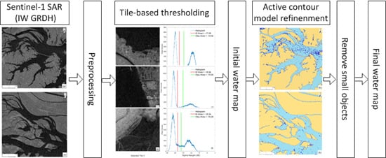
The HAWE method consists of four main parts (in Figure 2): (a) SAR preprocessing using the SNAP toolkit, (b) automatic tile-based thresholding and deriving initial water map as heuristic inputs, (c) applying the ACM to refine the initial water map, and (d) removing small objects from the refined water map and outputting the final water classification. Then, we compare the water map extracted by the HAWE with the Sentinel-2 MSI reference data, which is derived by steps 6 and 7, and the compare process is accomplished by step 8. The SNAP toolkit is used for preprocessing Sentinel 1 or 2 data, and the Matlab 2017a software is applied for water map extraction and accuracy evaluation.

3.1. Preprocessing of Sentinel-1 SAR

In this step, Sentinel-1 datasets with Level-1 GRDH products (10 m) are processed by the SNAP toolkit, including geometric correction, radiometric correction, de-speckle filtering, linear to sigma naught (dB) transformation, and finally, extracting the image of the study area, as outlined in Figure 1. The purpose of step 1 SAR preprocessing is to derive de-noised, geometric, and radiometric corrected SAR images for the study areas. The graph processing tool (GPT) embedded in the SNAP toolkit allows the aforementioned sub-steps to be processed automatically. Geometric correction, combined with SRTM DEM data, is aimed to correct the terrain distortion and to improve the geolocation accuracy. Afterwards, the Sentinel-1 SAR scene is range-doppler terrain corrected and projected to the WGS-84 geographical coordinate system. We set the Sentinel-2 MSI as the reference image and select the ground control points on both images to co-register the Sentinel-1 image by the polynomial model. The geometric corrected scene is calibrated to the backscatter coefficients and exported as sigma naught images [6]. As the VV-polarized image can generate better results [28] than HH polarized one, only the VV-polarized output option is selected. The calibrated scenes are filtered to reduce the inherent speckle noise, using the Lee Sigma filter with a 7 × 7 window and the sigma with 0.9. The backscattered coefficients are then converted into decibel-scale (dB) and the images of the study area are cropped in the following steps. In summary, the result of this step is geometric corrected, re-projected and calibrated backscatter coefficients (in dB) images for the study area.

3.2. Automatic Tile-Based Thresholding and Initial Water Map Classification

Step 2 “Automatic thresholding” and step 3 “Initial water map classification” are used to derive the heuristic water map for the next processing steps, with the former step obtaining the threshold and the latter classifying water and non-water regions. We at first divide the whole image into different tiles and then select qualified tiles to compute the optimal local thresholds, which is then averaged to generate the initial water map (classification). To choose qualified tiles, a bi-level quad tree structure [28] is applied and the detail steps are listed as follows:

(i) Tiling the entire scene into different tiles (batches or blocks) $L_i^{+}\left(i=1,2,\dots ,K\right)$ with the size of $c\times c$ pixels, which are called parent level tiles, and each parent tile is further separated into four children sub-tiles $L_{ij}^{-}\left(j=1,2,3,4\right)$ and each sub-tile has a size of $c/2\times c/2$ pixels.

(ii) Selecting the initial $N_1$ candidate tiles. Firstly, for each parent tile $L_i^{+}(i=1,2,\dots ,K)$, the mean backscatter intensity $\mu (L_{ij}^{-})$ for each sub-tile $L_{ij}^{-}(j=1,2,3,4)$ is calculated. The standard deviation of these $\mu (L_{ij}^{-})$ values, denoted as $\sigma (L_i^{+})$, are sorted in ascending order. The parent tiles with $\sigma (L_i^{+})$ value above 95% quantile and mean intensity less than the mean of all parent tiles are finally selected as the initial $N_1$ candidate tiles, because these two criterions assure the selected tiles of having large spatial heterogeneity and more than one semantic class [22,28]. As for the number of $N_1$, there are usually enough $N_1$ tiles be chosen in this step and its value ranges from 22 to 51 [21], which is sufficient to fulfill the success of the following steps. If $N_1$ is too small, it is recommended to reduce the size of both parent tiles and sub-tiles to its half and also decrease the quantile from 95 to 90%, which allows many more candidate tiles to be selected.

(iii) Selection of $N_2$ qualified tiles for thresholding. The standard deviation $\sigma (L_n^{+}),n=1,2,\dots ,N_1$ of the initial $N_1$ candidate tiles are sorted in descending order. The tiles with the highest standard deviation and the average backscattered intensity less than the mean value of all $N_1$ tiles are chosen as the qualified tiles. As suggested in previous studies [21,28], $N_2=5$ is adopted in this study.

(iv) Deriving the optimal threshold from $N_2$ qualified tiles and generating the initial water map. For each qualified tile, the KI thresholding method [26] is applied to derive the thresholds, which are then averaged to obtain the optimal threshold. The initial water map is derived by thresholding on the entire scene with the optimal threshold.

3.3. Active Contour Refinement of Initial Water Map

There are usually some water pixels missing in the initial water map that need to be refined. Step 4 “Active contour refinement for initial water map” is designed to accomplish this goal, which can delineate accurate boundaries between water and non-water and derive convincing water maps. The ACM model can automatically detect the exterior and interior boundaries and stop the contours at weak or blurred edges, hence, it is ideal for further refinement of the initial water map. According to the ACM model [29], the level set formulation is given as follows, in which the contours between water and non-water are evolved in each iteration step:

$$\frac{\partial \varphi }{\partial t}=spf(I(x))\cdot \alpha \left|\nabla \varphi \right|,x\in \Omega$$

(1)

where $\Omega$ is the domain for a given image $I$; $\nabla$ is the gradient operator to compute the image gradient for each pixel; $\alpha$ controls the smoothness of zero level set (the boundaries between water and non-water areas); $\varphi$ is the level set function to define the status of water or non-water areas and the boundaries between them.

$spf(\cdot )$ is the signed pressure force (SPF) function, which modulates the signs of the pressure force. As a result, the water and non-water boundaries will shrink when pixels are located outside the water area and expanded when inside the water area.

$$spf(I(x))=\frac{I(x)-\frac{c_1+c_2}{2}}{\max (\left|I(x)-\frac{c_1+c_2}{2}\right|)}$$

(2)

where $c_1$ and $c_2$ are the average intensities of the inner contour (the water area) and external contour (the non-water area), respectively, which can be derived by:

$$c_1(\varphi )=\frac{{\int }_{\Omega }I(x)\cdot H(\varphi )dx}{{\int }_{\Omega }H(\varphi )dx}$$

(3)

$$c_2(\varphi )=\frac{{\int }_{\Omega }I(x)\cdot (1-H(\varphi ))dx}{{\int }_{\Omega }(1-H(\varphi ))dx}.$$

(4)

Herein $H(\varphi )$ is the Heaviside function, which smoothes the distributions of $\varphi$, and its regularized version is given as:

$$H_{\epsilon }(z)=\frac{1}{2}(1+\frac{2}{\pi }\arctan (\frac{z}{\epsilon })).$$

(5)

The parameter $\epsilon$ is used to extract the accurate contour. According to Zhang [29], $\epsilon =1.5$ is recommended for extracting the accurate contours.

The ACM model [29] contains six steps as detailed below:

(1) Initializing the level set function $\varphi$ with the initial water map as

$$\varphi (x,t=0)=\{\begin{array}{cc}\hfill -1,& x\in {\Omega }_0-\partial {\Omega }_0\hfill \\ \hfill 0,& x\in \partial {\Omega }_0\hfill \\ \hfill 1,& x\in \Omega -{\Omega }_0\hfill \end{array}$$

(6)

where ${\Omega }_0$ is the water pixels extracted from Sentinel-1 SAR, and $\partial {\Omega }_0$ is the boundary of ${\Omega }_0$.

(2) In order to handle large scenes and accelerate the computation speed, the SAR image is evenly split into blocks with a size of 2 × 2 k pixels. For each block, do steps from (3) to (6) until all blocks are processed.

(3) Compute $c_1(\varphi )$ and $c_2(\varphi )$ for each block under processing using Equations (3) and (4).

(4) Evolve the level set function using Equation (1).

(5) Regularize the level set function with a Gaussian filter (with the standard deviation $\sigma =1$ and a kernel size of $K=5$) by an image convolution operator.

(6) Continue step (2) until the number of iterations reaches 30 or the level set function has converged.

3.4. Removing Small Objects to Derive the Final Results of Classification

After refining the initial water map, the water and non-water pixels can be divided by setting $\varphi <0$. However, there are still some small objects (islands) of water or land that should be rectified or eliminated. Step 5 “Remove small objects and output final results" is employed to complete this task. According to [3,22], we set the minimum size of small lakes or islands as 300 pixels, which means that any small lakes or islands with an area measured by the number of pixels less than 300 will be removed.

3.5. Processing of Sentinel-2 MSI and Performance Evaluation

The aim of step 6 “MSI preprocessing” is to obtain the subset of Sentinel-1 MSI images. Step 7 “derivation reference data” is used to obtain the water map as reference data for SAR extraction evaluation, which is done in step 8 “Water extraction accuracy evaluation”. The Sentinel-2 MSI Level-1C products are radiometric corrected and provide the Top-Of-Atmosphere (TOA) reflectance. However, there are still residual atmospheric effects in TOA reflectance data and need to be eliminated. The Sen2Cor [35], a Level-2A (L2A) processor embedded in the SNAP toolkit, is used to remove the atmospheric effects and derive the Level-2A surface reflectance products. Then they are co-registered with the corresponding Sentinel-1 SAR image to obtain the subset image of the study area.

The automated water extraction index (AWEI) [13] is applied to Sentinel-2 MSI to extract water inundations as reference data. Two AWEI forms, AWEInsh, and AWEIsh, can be used in different situations. According to Feyisa [13], the separation of water and non-water bodies can be done by applying AWEIsh coefficients that force non-water pixels below 0 and water pixels above 0.

$${AWEI}_{sh}={\rho }_{band2}+2.5\times {\rho }_{band3}-1.5\times ({\rho }_{band8}+{\rho }_{band11})-0.25\times {\rho }_{band12}$$

(7)

where $\rho$ represents the surface reflectance of Sentinel-2 MSI. The water extent extracted by Sentinel-2 MSI using the AWEIsh index is used as the reference water inundations in this study because it is good at extracting water maps from MSI with good performance [13,36].

4. Results

4.1. Extracted Water Inundation Areas

The extracted water inundation areas for test sites A and B (as illustrated in Figure 1) are shown in Figure 3 and Figure 4, respectively. As can be seen, most of the water inundation areas in the validation sites A and B were correctly extracted and the refined contours of water and non-water areas are much more accurate, especially for Figure 3c and Figure 4c,e,g. There are still some narrow rivers that are missed in the detected results because these objects are excluded from the initial water map and are prone to be neglected when the contours of water are evolving [29]. In addition, these rivers are too narrow to be detected by active contour-based refinement, and the backscatter intensities of these objects are also relatively higher than the derived overall optimal threshold and thus are considered as non-water objects.

In theory, open water areas often have a relatively smooth surface and produce much less backscattered signals to the SAR sensor. So, the water bodies generally appear darker color than non-water objects, such as built areas and forests. Thus, it is easy to separate water from non-water by thresholding. However, due to the inherent speckle noise, weather conditions, and acquisition time, the initial water map derived by thresholding could fail to detect certain water bodies, such as the small ponds, reservoirs, and narrow rivers. As a result, the detected initial water map tends to underestimate water inundation areas, as shown in Figure 3. Beginning with the initial water map, the desired water inundation areas, and contours of water bodies are eventually derived by the active contour refinement method.

The functions of applying the active contour model to the initial water map are mainly marked in two aspects. Firstly, comparing with some mathematical morphology methods, the active contour model method can refine the water and non-water boundaries as more accurate and closer as possible to the natural reality, no matter whether they are weak or blurred edges. Secondly, the evolution process of the active contour model method can combine some small water objects with similar backscatter intensity in open water areas, which seems reasonable and is in conformity with real situations. These small water objects often exist because of the inherent speckle noise in SAR data or small water waves induced by wind.

4.2. Comparison and Performance Evaluation

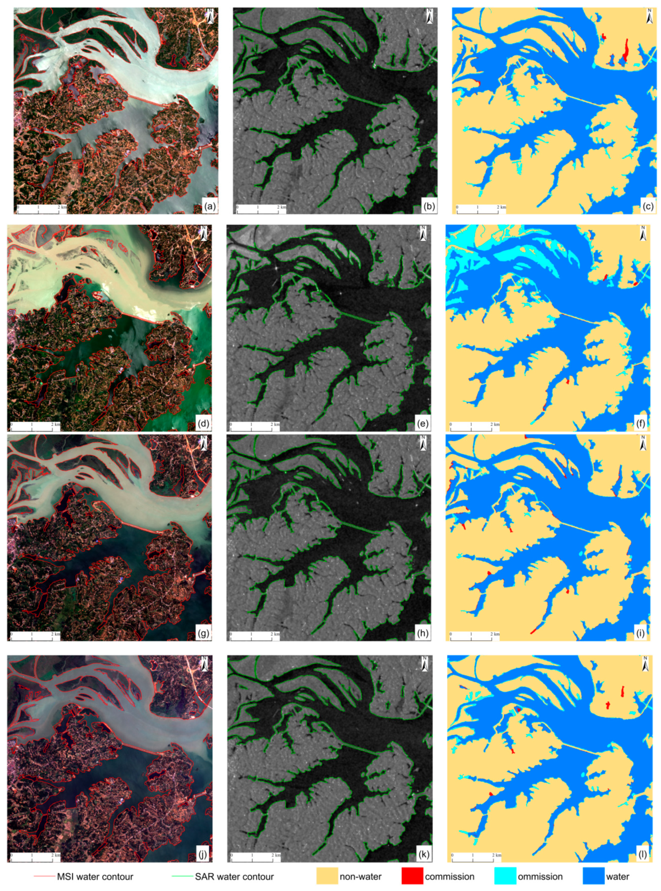
The water and non-water contours for test sites A and B extracted from Sentinel-1 SAR and Sentinel-2 MSI, as well as the water classification overlay, are shown in Figure 5 and Figure 6 for comparison. The Sentinel-2 MSI extracted water map is set as the reference data because reliable water information can be derived by the AWEI method and its spatial resolution (10 m) is finer than that of Sentinel-1 SAR data, which was upsampled from 20 × 22 m to 10 × 10 m. When they were overlaid, most of the water inundation areas are consistent with each other. While there are still some differences between them, especially for the water and non-water edges, isolated islands, or narrow rivers, which are prone to be inundated in different seasons and are failed to be detected as discussed in Section 4.1. Due to a flooding event, there were dramatic surface water discrepancies between extracted results from the Sentinel-1 SAR (acquired on 22 July 2017) and the Sentinel-2 MSI reference data (acquired on 17 July 2017), as shown in Figure 5f and Figure 6f. As reported in [37], there was a long persistent heavy rain in Hunan province since 22 June 2017, which had induced severe flooding around the entire province, including the Dongting Lake (China). On 17 July 2017, when the Sentinel-2 MSI scene was acquired, the floods were receded slowly but still with lots of lands and islands inundated. While on 22 July 2017, when the Sentinel-1 SAR was acquired, the flood receded completely with pre-inundated lands and islands exposed again. The commission surface waters mainly occurred in narrow rivers or edges and ends of large open water areas for the validation site A. The omission surface waters rarely occurred for the validation site A, which occurred frequently within the edges and ends of large open water areas for the validation site B. However, most of these commission surface waters were actual water bodies by visual interpretation checking, which were underestimated by the AWEIsh method in the reference data.

To sum up briefly, the differences between the extracted surface water from Sentinel-1 SAR and the reference data are mainly caused by the following reasons: (i) The inconsistent spatial resolution between the Sentinel-1 SAR (nominal 10 m) and Sentinel-2 MSI (real 10 m), in which images with coarse spatial resolution are prone to produce mixed pixel problems for the water and non-water edges; (ii) there are 4–5 days of delay for image acquisition. Though it is reasonable to assume that there is insignificant change in water inundation areas in such a short time period, it is inevitable that considerable changes happen during different time periods, especially for a flooding event period, as shown in Figure 5f and Figure 6f; (iii) the AWEIsh method may fail to detect the surface water under some circumstances, which may also yield differences; (iv) some water bodies are excluded from the initial water map because its backscatter intensities are relatively higher than the finally derived optimal threshold. The higher backscatter intensity may also hinder the water contours’ evolution process and led to misclassification.

Taking the Sentinel-2 MSI based water extraction as the reference data, the Sentinel-1 SAR based water extraction was pixel-wisely compared to determine several quantitative metrics, including the producer’s accuracy (PA), user’s accuracy (UA), overall accuracy (OA), and Kappa coefficient (K). The definitions of these quantitative metrics are given as follows [38,39,40]:

$$\mathrm{OA}=\frac{{\mathrm{P}}_{11}+{\mathrm{P}}_{22}}{N}\times 100\%$$

(8)

$$\mathrm{PA}\_water=\frac{{\mathrm{P}}_{11}}{{\mathrm{P}}_{11}+{\mathrm{P}}_{21}}\times 100\%$$

(9)

$$\mathrm{PA}\_\mathrm{non}\text{-}water=\frac{{\mathrm{P}}_{22}}{{\mathrm{P}}_{12}+{\mathrm{P}}_{22}}\times 100\%$$

(10)

$$\mathrm{UA}\_water=\frac{{\mathrm{P}}_{11}}{{\mathrm{P}}_{11}+{\mathrm{P}}_{12}}\times 100\%$$

(11)

$$\mathrm{UA}\_\mathrm{non}\text{-}water=\frac{{\mathrm{P}}_{22}}{{\mathrm{P}}_{21}+{\mathrm{P}}_{22}}\times 100\%$$

(12)

$$\mathrm{K}=\frac{N{\displaystyle \sum _{i=1}^2{\mathrm{P}}_{ii}}-{\displaystyle \sum _{i=1}^2{\mathrm{P}}_{i+}\ast {\mathrm{P}}_{+i}}}{N^2-{\displaystyle \sum _{i=1}^2{\mathrm{P}}_{i+}\ast {\mathrm{P}}_{+i}}}$$

(13)

where, P₁₁, P₁₂, P_21, and P₂₂ construct an error matrix (confusion matrix), which denotes, respectively, the number of water pixels on both the SAR extraction and the reference data, the number of water pixels on SAR extraction which are non-water pixels on the reference data, the number of non-water pixels on the SAR extraction which are water pixels on the reference data, and the number of non-water pixels on both the SAR extraction and the reference data; ${\mathrm{P}}_{i+}$ and ${\mathrm{P}}_{+i}$ are the marginal totals of row $i$ and column $i$ for the error matrix, respectively; $N={\mathrm{P}}_{11}+{\mathrm{P}}_{12}+{\mathrm{P}}_{21}+{\mathrm{P}}_{22}$ is the total number of pixels.

Table 2. Quantitative metric values of the proposed heuristic and automatic water extraction (HAWE) method for two selected test sites and the whole study area *.

Test Sites	SAR Date (dd/mm/yyyy)	OA (%)	PA Water (%)	UA Water (%)	PA Non-Water (%)	UA Non-Water (%)	K
Site A	23/05/2017	95.54	99.50	89.32	93.30	99.70	0.91
	22/07/2017	78.15	100	64.01	64.27	100	0.58
	20/09/2017	94.91	99.68	88.04	92.13	99.80	0.89
	09/10/2018	94.90	99.88	87.12	92.29	99.93	0.89
Site B	23/05/2017	96.35	98.68	92.08	94.97	99.18	0.92
	22/07/2017	90.51	99.37	81.07	84.65	99.51	0.81
	20/09/2017	97.21	98.41	94.67	96.43	98.95	0.94
	09/10/2018	96.66	99.12	92.23	95.27	99.48	0.93
Whole Study Area	23/05/2017	96.71	85.65	94.21	98.94	97.16	0.88
	22/07/2017	93.31	75.44	98.92	99.70	91.90	0.81
	20/09/2017	96.80	84.80	97.27	99.47	96.71	0.89
	09/10/2018	97.41	86.95	95.51	99.27	97.72	0.90

* Descriptions: (a). Each row shows the corresponding quantitative metric values of water extraction from the HAWE method on different test sites and dates. (b). The 1st column ’Test Sites’ shows the corresponding test site, including Site A, Site B, and the whole study area, as shown in Figure 1; the 2nd column gives the data acquisition date for Sentinel-1 SAR data. (c). The 3rd to the 8th columns represent the relevant metric values in terms of producer’s accuracy (PA) water, user’s accuracy (UA) water, overall accuracy (OA), PA non-water, UA non-water, and Kappa coefficient (K) as defined in Equations (8)–(13).

shows the comparison results for the sites A, B, and the whole study area. In Table 2, there are minor differences in terms of the classification accuracy for test site A, with the OA varying between 94.90% and 95.54% and the K ranging from 0.89 to 0.91, except for the date 22 July 2017. While for the validation site B, the OA (between 90.51% and 97.21%) and K (between 0.81 and 0.94) are both slightly higher than that of the test site A. This is because most of the surface water is fully protected by natural dikes and the water inundation areas for the validation site B are much more stable than site A, hence the evaluation accuracies for validation site B are considerably higher. When compared to Sentinel-2 MSI water extraction results, the root mean squared error (RMSE) of water area extracted by Sentinel-1 SAR is 11.65 km² on site A and 4.94 km² on site B for all dates. The main reason is that there are some narrow rivers or small reservoirs that are not detected due to the low backscatter intensity or exclusion in the initial water map.

With respect to the water and non-water classification accuracy over the whole study area, the OA and K values derived on different dates are generally consistent, varying within 94.32–96.8% and 0.80–0.89, respectively, where it seems only the PA water values show a slightly larger variability than others. The statistical evaluations for the study area indicate that the proposed method can obtain desired water maps for the Sentinel-1 SAR time series, where different backscattered intensities help to make the water extent separation a hard problem.

5. Discussion

5.1. The Effects of Different Thresholding Methods on Accuracy

The selected tiles, which are generally located in water and non-water junctions and usually show bimodal histogram characteristics, are used for deriving the overall optimal threshold for the entire scene. For comparison, the Otsu [27] thresholding is also applied to derive the optimal threshold. The Otsu thresholding finds the threshold value when the sum of the foreground and background spreads is at its minimum. It involves iterating through all the possible threshold values to calculate a measure of spread for the pixel levels at both sides of the threshold. KI thresholding method is a minimum error thresholding algorithm which minimizes the probability of classification error. As water backscatter intensity is relatively low, the corresponding SAR image can be usually characterized by a bimodal intensity histogram. The Sentinel-1 SAR dataset acquired on 23 May 2017 is selected as an example to show the effect of the different tile-based thresholding on generating the initial water map. The final selected qualified tiles and their corresponding intensity histograms and the optimal local thresholds for each tile are shown in Figure 7. There are a certain amount of water and non-water areas in the selected tiles which show a significant bimodal histogram. As for the tile-based optimal thresholds, there are significant differences between those from the KI and Otsu methods. More specifically, the thresholds derived by the KI method are generally less than that of the Otsu method.

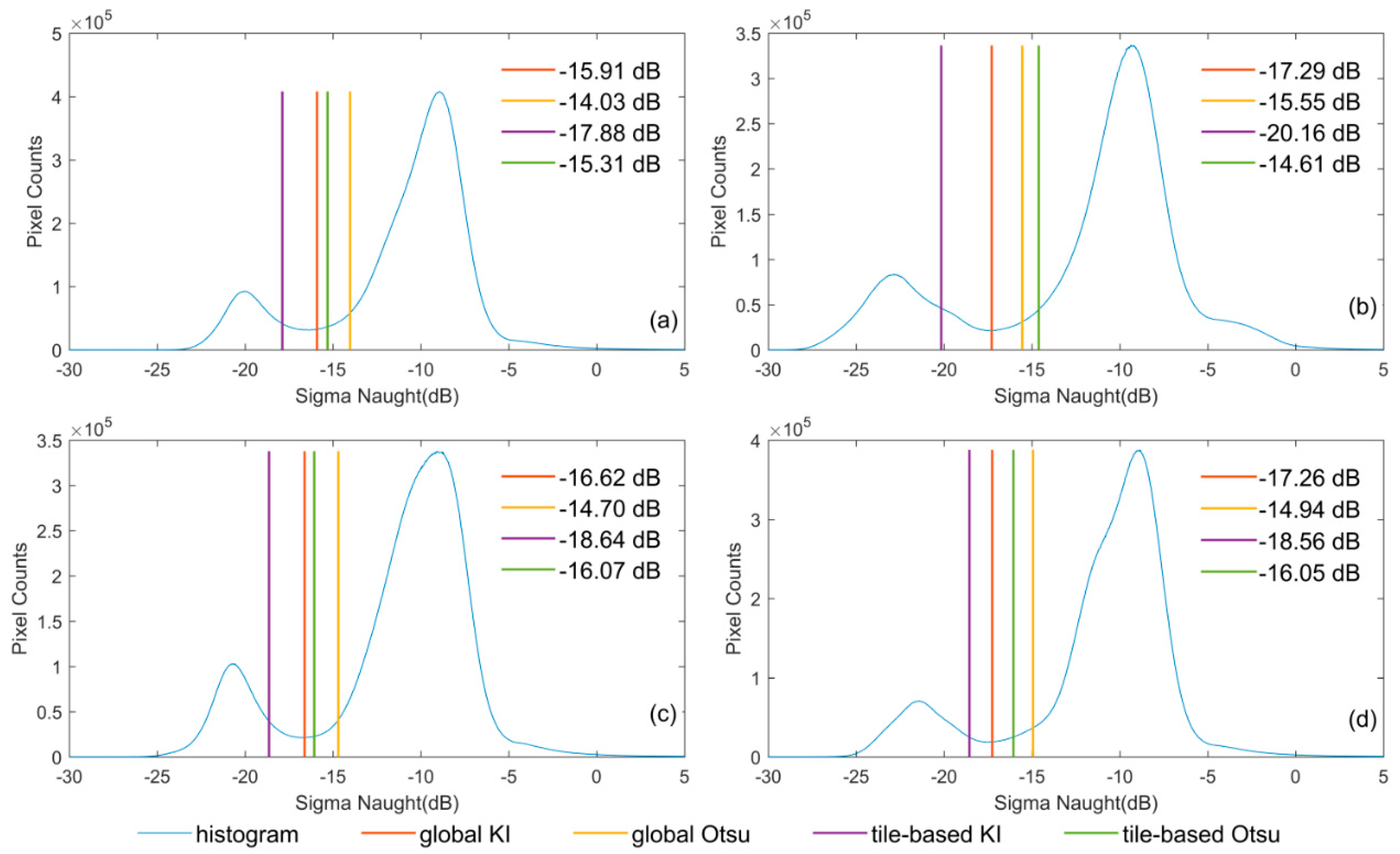
The KI and Otsu methods applied directly to the entire image, named the global KI and global Otsu method respectively, are used for comparison with the tile-based KI and Otsu methods. Relevant results are compared in Figure 8. As seen, there are significant differences among these results, where the thresholds derived by tile-based KI have the lowest intensities, followed by the global KI method, while both the global and tile-based Otsu methods have yielded higher thresholds than that of the KI method. The global Otsu method can always obtain higher thresholds than tile-based Otsu, except for Figure 8b. The final derived optimal thresholds vary from different dates for all methods. From the visual perspective of bimodal histograms, the global KI method has better results. However, the tile-based KI method, whose values are relatively lower than that of any other methods, can derive water body pixels with the highest degree of confidence. The global Otsu and tile-based Otsu methods, whose values are obviously higher than previous studies [5,6,21,28], are prone to misclassify some non-water pixels as water, which will overestimate surface waters and bring risks to the active contour refinement process.

The final results of water classification derived by the HAWE method, in which the global or tile-based KI and Otsu methods are used to generate the initial water map, are compared with the reference data. According to the results shown in

Table 3. Mean (standard deviation) quantitative metric values of water extraction results for the whole study area with the initial water map derived by different thresholding *.

Quantitative Metrics	Global KI	Global Otsu	Tile-Based KI	Tile-Based Otsu
OA (%)	94.88(2.16)	88.97(3.05)	96.06(1.86)	95.00(2.84)
Kappa	0.82(0.06)	0.68(0.10)	0.87(0.04)	0.82(0.08)
PA water (%)	84.34(4.12)	62.74(10.72)	83.21(5.25)	90.38(2.34)
PA non-water (%)	97.00(3.00)	98.35(0.99)	99.34(0.32)	95.82(3.75)
UA water (%)	86.45(11.02)	93.08(4.19)	96.48(2.06)	81.32(12.85)
UA non-water (%)	96.86(0.74)	88.14(3.12)	95.87(2.68)	98.26(0.36)

* Descriptions: (a). Each row shows the quantitative metric values from different initial water maps derived from four approaches for the whole study area. (b). The 1st column ‘Quantitative Metrics’ shows different metrics as defined in Equations (8)–(13). (c). The 2nd to the 5th columns represent the corresponding mean (standard deviation) metric values for initial water maps derived from different approaches.

, for the OA and the Kappa coefficient K, the tile-based KI generally outperforms others, with a relatively higher mean accuracy (95.22% for OA and 0.83 for K) and a lower standard deviation (1.12% for OA and 0.04 for K), followed by the global KI and tile-based Otsu, while the global Otsu has the lowest accuracy. This means that although a lower threshold was derived by the tile-based KI method, the final water classification still has good results and seems more stable than other thresholding methods. For PA and UA of water and non-water, there are significant differences among different thresholding methods and tile-based thresholding methods can produce better results than that of global thresholding.

5.2. The Effect of Iterations on Water Boundary Evolution

When the ACM model was applied to refine the initial water classification map, two important parameters including the $\alpha$ and the iteration number need to be further discussed. The parameter $\alpha$ controls the smoothness of the zero-level set (contours). Empirically we set $\alpha =20$ in this study as it can result in stable shapes for water inundation contours. In contrast to $\alpha$, the iteration number, which controls the evolutions of level set function and checks up whether water boundaries have converged, affects the final results to a great extent.

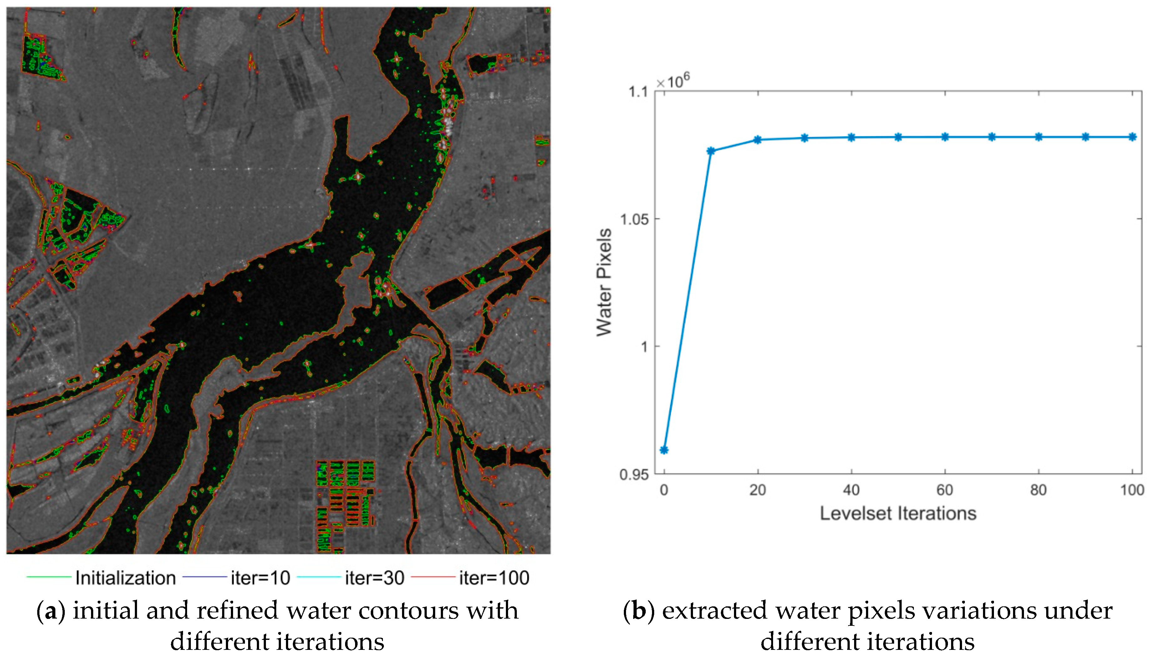
To further evaluate how this parameter affects the final results of extracted water maps, we selected an area in this study area and conducted experiments by setting different numbers of iterations varying from 10 to 100 with an interval of 10, and the results are shown in Figure 9 for comparison. Obviously, the initial water map derived by step 3, as shown in Figure 9a, has underestimated the water extent, where the water and non-water boundaries are also inaccurate. The accurate boundaries between water and non-water can be easily derived by introducing the ACM into the refinement process, as it evolves the edges by computing the image gradient during the iterations. The evolution process converges fast after a few iterations and the water and non-water boundaries are evolved to desired shapes, which can also be found in Figure 9b where the number of extracted water pixels keeps stable after 30 iterations. This is due to the fact that the initialization of water classification has detected most of the confident water inundations, which can accelerate the converge process in refinement and can also further enhance the accuracy of water and non-water boundaries.

5.3. Comparisons with Other Methodologies

To compare the proposed approach with other methodologies, we choose the tile-based KI thresholding (T-KI) [21,26], the image-based KI thresholding method [26], the ACM method [29], and the histogram-based thresholding method (HTM) [3,22] to extract the water maps followed by removal of small objects for comparison. In the ACM method, the iterations are 200 times and other parameters are kept the same as the proposed method. In the HTM, pixels with intensities, less than −18 dB are regarded as confident water and larger than −14 dB are classified as confident land where the kernel size in morphological operations is 3 × 3 window. The OA and K measurements are used to evaluate the results on two selected test sites and the results are compared in

Table 4. The OA and K accuracies of water extraction results derived by different methods for two selected test sites *.

Test Site	SAR Date (dd/mm/yyyy)	OA (%)					K
		T-KI	KI	ACM	HTM	HAWE	T-KI	KI	ACM	HTM	HAWE
Site A	23/05/2017	91.86	94.46	84.94	93.57	95.54	0.82	0.88	0.70	0.86	0.91
	22/07/2017	68.84	78.79	82.24	77.49	78.15	0.43	0.59	0.64	0.57	0.58
	20/09/2017	92.69	95.69	87.57	95.07	94.91	0.85	0.91	0.75	0.90	0.89
	09/10/2018	92.67	94.54	85.97	95.03	94.90	0.84	0.88	0.72	0.89	0.89
Site B	23/05/2017	94.37	95.78	92.32	96.04	96.35	0.88	0.91	0.84	0.92	0.92
	22/07/2017	61.91	89.72	87.44	89.27	90.51	0.22	0.79	0.75	0.78	0.81
	20/09/2017	85.57	97.02	92.29	94.33	97.21	0.68	0.94	0.84	0.88	0.94
	09/10/2018	91.71	96.45	92.48	95.56	96.66	0.82	0.92	0.85	0.90	0.93

* Descriptions: (a). Each row shows the quantitative evaluations, OA and K, of different water map extraction methods on different dates for Site A or Site B. The bold figures indicate the highest values for OA or K. (b). The 1st column specifies the corresponding test site, and the 2nd column ‘SAR Date’ is the data acquisition date for the SAR data. (c). From the 3rd to the 12th columns are the OA and K values for corresponding methods including T-KI, KI, ACM, HTM, and HAWE, respectively.

.

As seen from Table 4, the tile-based thresholding (T-KI) can derive a confident water map but with relatively low accuracy. This is because the selected tiles used for determining threshold usually contain enough water and non-water pixels, but they cannot separate all water pixels from non-water pixels. Due to the heterogeneity and complexity of the ground surface, the accuracy of the water map by the ACM method is still not good enough and thus needs to be improved. The KI thresholding can produce good results but the edges between water and non-water are hard to be accurately detected. The HTM method is easy for implementation and is efficient to derive water maps with comparable accuracy, but the corresponding empirical thresholds for separating water and non-water as well as the morphological kernel size for further refinement need to be decided carefully in different situations. The HAWE, by combining the advantages of T-KI and ACM, can significantly improve the results and keep the OA and K metrics the highest for different dates on the two test sites. It suggests that the proposed method can produce more accurate and robust results for water map extraction using the Sentinel-1 SAR times series regardless of the changes of dry or rainy seasons.

5.4. Advantages and Disadvantages

Though optical sensors can be used to derive convincing water inundations, they are severely affected by bad weather conditions, such as the cloud, haze, and rain, making it hard for persistently monitoring the surface water changes with a relatively high temporal resolution. For the study area, the available optical imageries with few clouds and high quality are quite rare. Whereas, SAR is capable of acquiring data independent on weather and daylight and providing reliable information for surface water. Note SAR backscatter intensities for the same water zones may vary from each other during different seasons, making it difficult for dividing water and non-water with quite a similar backscatter intensity. The proposed approach can tackle this limitation and performs quite well in the study area for deriving accurate water inundation maps. There are some advantages to the proposed method we would like to highlight. Firstly, the initial water map derived by the tile-based thresholding assures confident water areas are included and thus can be used as heuristic inputs for further water map refinement, which avoids misclassifying the water body, expanding the water boundary, and speeding up the convergence process in the refinement phase. Secondly, it is a fully automated method with only a few predefined parameters, and only one auxiliary data is needed. Furthermore, most inundated water areas can be correctly extracted owing to the combination of tile-based thresholding and active contour model, and it is also resistant to the inherent speckle noise in Sentinel-1 SAR. In addition, the contours (boundaries) between water and non-water areas can be accurately extracted because the ACM model uses image gradient information to evolve the contours, which is better and much more accurate than morphological operations without any prior knowledge of the images. Finally, our algorithm is simple, easy to implement, and quite efficient. As the initial water classification was derived by tile-based thresholding, most water and non-water areas have been correctly extracted, and thus the convergence rate can be accelerated when conducting evolutions of the level set function. To further speed up the computations, the level set function evolution can be implemented in parallel on the divided blocks.

Missing detection of water inundation areas occasionally occurs in our approach because some water bodies are excluded in the initialization level set function. As mentioned in Section 4.2, when the tile-based thresholding was applied to the entire scene, some regions such as small ponds, pools, reservoirs, and narrow rivers, whose backscatter intensity is relatively higher than the final optimal threshold, are not classified as initial water bodies and are prone to be classified as non-water in the final results of water classification. To overcome this problem, it is feasible to raise the threshold to include more water pixels in the initial water classification. While some non-water objects with similar backscatter will also be classified as water bodies. Actually, for large study areas such as Dongting Lake (China), these small ponds, pools, reservoirs, and narrow rivers are not important and can be neglected.

6. Conclusions

In this study, a heuristic and automatic water extraction (HAWE) approach for the extraction of water inundation area data was presented and tested on the Dongting Lake plain (China), where the topography is mostly flat plains and the water inundation areas are prone to change with different seasons due to the seasonal precipitation variations in this drainage basin. By adopting the tile-based thresholding, an initial water map with confident water pixels can be derived as heuristic inputs for further refinement. In the refinement process, the ACM model makes use of the statistic information from the SAR image itself to evolve the contours between water and non-water areas. This process can avoid empirical parameter settings for morphological operations case by case and derive a more accurate extraction of water inundations. The entire process in the HAWE can be implemented with few predefined parameters and can automatically generate the final water classification map for the SAR time series.

The performance of the proposed method has been evaluated using two test sites within the Dongting Lake plain (China). The results have indicated that the proposed method is able to achieve satisfying classification results in terms of the overall accuracy (between 78.15% and 97.21%) and the Kappa coefficient (ranging from 0.58 to 0.94) of water extraction. We also compared the proposed approach with other methods, such as the direct tile-based method and ACM without initial water map, and the results also show that our method can outperform several other methods listed in this study.

The limitation of this approach is that it may fail to detect some small water bodies or narrow rivers with relatively higher backscatter intensities, because neither initial water map nor the evolution process could identify them as water pixels. Raising the threshold may help to include these water bodies in the initial water map and solve the problem to some extent, however, it may also introduce non-water objects into the final results. In fact, for water inundation areas monitoring at large study areas, these small ponds, pools, reservoirs, and narrow rivers can be reasonably neglected due to their low importance as we mainly concern about the change analysis of the surface water for the overall study area.

References

- Palmer, M.; Ruhi, A. Measuring Earth’s rivers. Science 2018, 361, 546–547. [Google Scholar] [CrossRef] [PubMed]
- Martinis, S.; Twele, A.; Voigt, S. Towards operational near real-time flood detection using a split-based automatic thresholding procedure on high resolution TerraSAR-X data. Nat. Hazards Earth Syst. Sci. 2009, 9, 303–314. [Google Scholar] [CrossRef]
- Gstaiger, V.; Huth, J.; Gebhardt, S.; Wehrmann, T.; Kuenzer, C. Multi-sensoral and automated derivation of inundated areas using TerraSAR-X and ENVISAT ASAR data. Int. J. Remote Sens. 2012, 33, 7291–7304. [Google Scholar] [CrossRef]
- Pekel, J.-F.; Cottam, A.; Gorelick, N.; Belward, A.S. High-resolution mapping of global surface water and its long-term changes. Nature 2016, 540, 418. [Google Scholar] [CrossRef]
- Huang, W.; DeVries, B.; Huang, C.; Lang, M.; Jones, J.; Creed, I.; Carroll, M. Automated extraction of surface water extent from Sentinel-1 data. Remote Sens. 2018, 10, 797. [Google Scholar] [CrossRef] [Green Version]
- Martinis, S.; Plank, S.; Ćwik, K. The Use of Sentinel-1 Time-Series Data to Improve Flood Monitoring in Arid Areas. Remote Sens. 2018, 10, 583. [Google Scholar] [CrossRef] [Green Version]
- Pekel, J.F.; Vancutsem, C.; Bastin, L.; Clerici, M.; Vanbogaert, E.; Bartholomé, E.; Defourny, P. A near real-time surface water detection method based on HSV transformation of MODIS multi-spectral time series data. Remote Sens. Environ. 2014, 140, 704–716. [Google Scholar] [CrossRef] [Green Version]
- Wendleder, A.; Wessel, B.; Roth, A.; Breunig, M.; Martin, K.; Wagenbrenner, S. TanDEM-X Water Indication Mask: Generation and First Evaluation Results. IEEE J. Sel. Top. Appl. Earth Obs. Remote Sens. 2013, 6, 171–179. [Google Scholar] [CrossRef] [Green Version]
- Santoro, M.; Wegmüller, U.; Lamarche, C.; Bontemps, S.; Defourny, P.; Arino, O. Strengths and weaknesses of multi-year Envisat ASAR backscatter measurements to map permanent open water bodies at global scale. Remote Sens. Environ. 2015, 171, 185–201. [Google Scholar] [CrossRef]
- Carroll, M.L.; Townshend, J.R.; DiMiceli, C.M.; Noojipady, P.; Sohlberg, R.A. A new global raster water mask at 250 m resolution. Int. J. Digit. Earth 2009, 2, 291–308. [Google Scholar] [CrossRef]
- McFeeters, S.K. The use of the Normalized Difference Water Index (NDWI) in the delineation of open water features. Int. J. Remote Sens. 1996, 17, 1425–1432. [Google Scholar] [CrossRef]
- Xu, H. Modification of normalised difference water index (NDWI) to enhance open water features in remotely sensed imagery. Int. J. Remote Sens. 2006, 27, 3025–3033. [Google Scholar] [CrossRef]
- Feyisa, G.L.; Meilby, H.; Fensholt, R.; Proud, S.R. Automated Water Extraction Index: A new technique for surface water mapping using Landsat imagery. Remote Sens. Environ. 2014, 140, 23–35. [Google Scholar] [CrossRef]
- Du, Y.; Zhang, Y.; Ling, F.; Wang, Q.; Li, W.; Li, X. Water Bodies’ Mapping from Sentinel-2 Imagery with Modified Normalized Difference Water Index at 10-m Spatial Resolution Produced by Sharpening the SWIR Band. Remote Sens. 2016, 8, 354. [Google Scholar] [CrossRef] [Green Version]
- Rokni, K.; Ahmad, A.; Selamat, A.; Hazini, S. Water Feature Extraction and Change Detection Using Multitemporal Landsat Imagery. Remote Sens. 2014, 6, 4173–4189. [Google Scholar] [CrossRef] [Green Version]
- Musa, Z.N.; Popescu, I.; Mynett, A. A review of applications of satellite SAR, optical, altimetry and DEM data for surface water modelling, mapping and parameter estimation. Hydrol. Earth Syst. Sci. 2015, 19, 3755–3769. [Google Scholar] [CrossRef] [Green Version]
- Boergens, E.; Nielsen, K.; Andersen, O.B.; Dettmering, D.; Seitz, F. River Levels Derived with CryoSat-2 SAR Data Classification—A Case Study in the Mekong River Basin. Remote Sens. 2017, 9, 1238. [Google Scholar] [CrossRef] [Green Version]
- Biondi, F.; Tarpanelli, A.; Addabbo, P.; Clemente, C.; Orlando, D. Pixel Tracking to Estimate Rivers Water Flow Elevation Using Cosmo-SkyMed Synthetic Aperture Radar Data. Remote Sens. 2019, 11, 2574. [Google Scholar] [CrossRef] [Green Version]
- Cian, F.; Marconcini, M.; Ceccato, P.; Giupponi, C. Flood depth estimation by means of high-resolution SAR images and lidar data. Nat. Hazards Earth Syst. Sci. 2018, 18, 3063–3084. [Google Scholar] [CrossRef] [Green Version]
- Clement, M.A.; Kilsby, C.G.; Moore, P. Multi-temporal synthetic aperture radar flood mapping using change detection. J. Flood Risk Manag. 2018, 11, 152–168. [Google Scholar] [CrossRef]
- Martinis, S.; Kersten, J.; Twele, A. A fully automated TerraSAR-X based flood service. ISPRS J. Photogramm. Remote Sens. 2015, 104, 203–212. [Google Scholar] [CrossRef]
- Kuenzer, C.; Guo, H.; Huth, J.; Leinenkugel, P.; Li, X.; Dech, S. Flood mapping and flood dynamics of the Mekong Delta: ENVISAT-ASAR-WSM based time series analyses. Remote Sens. 2013, 5, 687–715. [Google Scholar] [CrossRef] [Green Version]
- Bazi, Y.; Bruzzone, L.; Melgani, F. Image thresholding based on the EM algorithm and the generalized Gaussian distribution. Pattern Recognit. 2007, 40, 619–634. [Google Scholar] [CrossRef]
- Sahoo, P.K.; Soltani, S.; Wong, A.K.C. A survey of thresholding techniques. Comput. Vis. Graph. Image Process. 1988, 41, 233–260. [Google Scholar] [CrossRef]
- Petrou, M.; Matrucceli, A. On the stability of thresholding SAR images. Pattern Recognit. 1998, 31, 1791–1796. [Google Scholar] [CrossRef]
- Kittler, J.; Illingworth, J. Minimum error thresholding. Pattern Recognit. 1986, 19, 41–47. [Google Scholar] [CrossRef]
- Otsu, N. A Threshold Selection Method from Gray-Level Histograms. IEEE Trans. Syst. Man Cybern. 1979, 9, 62–66. [Google Scholar] [CrossRef] [Green Version]
- Twele, A.; Cao, W.; Plank, S.; Martinis, S. Sentinel-1-based flood mapping: A fully automated processing chain. Int. J. Remote Sens. 2016, 37, 2990–3004. [Google Scholar] [CrossRef]
- Zhang, K.; Zhang, L.; Song, H.; Zhou, W. Active contours with selective local or global segmentation: A new formulation and level set method. Image Vis. Comput. 2010, 28, 668–676. [Google Scholar] [CrossRef]
- Sun, F.; Zhao, Y.; Gong, P.; Ma, R.; Dai, Y. Monitoring dynamic changes of global land cover types: Fluctuations of major lakes in China every 8 days during 2000–2010. Chin. Sci. Bull. 2014, 59, 171–189. [Google Scholar] [CrossRef]
- Zhou, Y.; Ma, J.; Zhang, Y.; Li, J.; Feng, L.; Zhang, Y.; Shi, K.; Brookes, J.D.; Jeppesen, E. Influence of the three Gorges Reservoir on the shrinkage of China’s two largest freshwater lakes. Glob. Planet. Chang. 2019, 177, 45–55. [Google Scholar] [CrossRef]
- Torres, R.; Snoeij, P.; Geudtner, D.; Bibby, D.; Davidson, M.; Attema, E.; Potin, P.; Rommen, B.; Floury, N.; Brown, M.; et al. GMES Sentinel-1 mission. Remote Sens. Environ. 2012, 120, 9–24. [Google Scholar] [CrossRef]
- Matgen, P.; Hostache, R.; Schumann, G.; Pfister, L.; Hoffmann, L.; Savenije, H. Towards an automated SAR-based flood monitoring system: Lessons learned from two case studies. Phys. Chem. Earth A/B/C 2011, 36, 241–252. [Google Scholar] [CrossRef]
- Drusch, M.; Del Bello, U.; Carlier, S.; Colin, O.; Fernandez, V.; Gascon, F.; Hoersch, B.; Isola, C.; Laberinti, P.; Martimort, P. Sentinel-2: ESA’s optical high-resolution mission for GMES operational services. Remote Sens. Environ. 2012, 120, 25–36. [Google Scholar] [CrossRef]
- Louis, J.; Debaecker, V.; Pflug, B.; Main-Knorn, M.; Bieniarz, J.; Mueller-Wilm, U.; Cadau, E.; Gascon, F. Sentinel-2 Sen2Cor: L2A processor for users. In Proceedings of the Living Planet Symposium, Prague, Czech, 9–13 May 2016. [Google Scholar]
- Fisher, A.; Flood, N.; Danaher, T. Comparing Landsat water index methods for automated water classification in eastern Australia. Remote Sens. Environ. 2016, 175, 167–182. [Google Scholar] [CrossRef]
- Li, J. The Flood Situation in the Yangtze River Basin Has Obviously Alleviated and the Emergency Response of the Fourth Level of the Flood Emergency Terminated by the Flood Control Headquarters. Available online: http://m.xinhuanet.com/2017-07/17/c_1121333933.htm (accessed on 9 August 2019).
- Cohen, J. A Coefficient of Agreement for Nominal Scales. Educ. Psychol. Meas. 1960, 20, 37–46. [Google Scholar] [CrossRef]
- Congalton, R.G. A review of assessing the accuracy of classifications of remotely sensed data. Remote Sens. Environ. 1991, 37, 35–46. [Google Scholar] [CrossRef]
- McHugh, M.L. Interrater reliability: The kappa statistic. Biochem. Med. 2012, 22, 276–282. [Google Scholar] [CrossRef]
Figure 1.
Dongting Lake plain (China) and two test sites. The Sentinel-1 scene with vertically transmitted vertically received (VV) polarization acquired on 23 May 2017.
Figure 2.
The diagram shows the workflow of the automated water inundation extraction and accuracy evaluation based on Sentinel-1 SAR and Sentinel-2 MSI.
Figure 3.
The initial water contours using tile-based KI thresholding method, refined water contours by the active contour model (ACM) model, and final extracted water inundations for validation site A; (a,c,e,g) show the initial and refined water contours, as well as the Sentinel-1 scene in VV polarization acquired on 23 May 2017, 22 July 2017, 20 September 2017, and 9 October 2018, respectively; (b,d,f,h) show the corresponding final water and non-water classification.
Figure 4.
The initial water contours using tile-based KI thresholding method, refined water contours by ACM model, and final extracted water inundations for validation site B; (a,c,e,g) show the initial and refined water contours, as well as the Sentinel-1 scene in VV polarization acquired on 23 May 2017, 22 July 2017, 20 September 2017, and 9 October 2018, respectively; (b,d,f,h) show the corresponding final water and non-water classification.
Figure 5.
The extracted water contours and final water classification overlays for Sentinel-2 MSI (as reference) and Sentinel-1 SAR for validation site A: (a,d,g,j) represent water contours derived by automated water extraction index (AWEI) method and true color compositions of Sentinel-2 MSI acquired on 18 May 2017, 17 July 2017, 15 September 2017, and 5 October 2018, respectively; (b,e,h,k) are extracted water contours using proposed method and Sentinel-1 SAR scene in VV polarization acquired on 23 May 2017, 22 July 2017, 20 September 2017, and 9 October 2018, respectively; (c,f,i,l) are overlays of the final water classification from Sentinel-1 SAR and Sentinel-2 MSI.
Figure 6.
The extracted water contours and final water classification overlays for Sentinel-2 MSI (as reference) and Sentinel-1 SAR for the test site B: (a,d,g,j) are water contours using the AWEI method and true color compositions of the Sentinel-2 MSI acquired on 18 May 2017, 17 July 2017, 15 September 2017, and 5 October 2018, respectively; (b,e,h,k) are extracted water contours using the proposed method and Sentinel-1 SAR scene in VV polarization acquired on 23 May 2017, 22 July 2017, 20 September 2017, and 9 October 2018, respectively; (c,f,i,l) are overlays of final water classification from Sentinel-1 SAR and Sentinel-2 MSI.
Figure 7.
The selected qualified tiles and the tile-based optimal threshold by different methods for Sentinel-1 SAR VV polarization acquired on 23 May 2017. (a,c,e,g,i) are finally selected qualified tiles with a size of 400 × 400 pixels; (b,d,f,h,j) are histograms and the tile-based optimal threshold corresponding to each selected qualified tile.
Figure 8.
Histograms and the corresponding optimal local thresholds derived by different methods for the Sentinel-1 SAR VV polarization scenes. (a–d) represents the Sentinel-1 SAR images acquired on 23 May 2017, 22 July 2017, 20 September 2017, and 9 October 2018, respectively.
Figure 9.
The refinement of initial thresholding results and extracted water pixels varying under different iterations.