Exploration of Indoor Barrier-Free Plane Intelligent Lofting System Combining BIM and Multi-Sensors

Abstract

Lofting is an essential part of construction projects and the high quality of lofting is the basis of efficient construction. However, the most common method of lofting currently which uses the total station in a multi-person cooperative way consumes much manpower and time. With the rapid development of remote sensing and robot technology, using robots instead of manpower can effectively solve this problem, but few scholars study this. How to effectively combine remote sensing and robots with lofting is a challenging problem. In this paper, we propose an intelligent lofting system for indoor barrier-free plane environment, and design a high-flexibility, low-cost autonomous mobile robot platform based on single chip microcomputer, Micro Electro Mechanical Systems-Inertial Measurement Unit (MEMS-IMU), wheel encoder, and magnetometer. The robot also combines Building Information Modeling (BIM) laser lofting instrument and WIFI communication technology to get its own position. To ensure the accuracy of localization, the kinematics model of Mecanum wheel robot is built, and Extended Kalman Filter (EKF) is also used to fuse multi-sensor data. It can be seen from the final experimental results that this system can significantly improve lofting efficiency and reduce manpower.

1. Introduction

The process of construction mainly includes construction preparation, project construction, project acceptance, etc. The lofting is included in the construction project and project acceptance. It is the process of interpreting construction plans and marking the location of points or axis. Lofting is performed to ensure a project is built according to engineering design plans [1,2] and it is an essential and basic link in building construction which runs through the whole construction project.

The quality of a project’s lofting depends on its efficiency and cost. In the early stages, limited by the lofting tools and methods, several operators were required to invest a lot of energy and time in lofting and calibration at the construction site. In the past decade, with the rapid development of surveying and mapping industry, the appearance of total station has greatly improved the lofting efficiency. As an instrument integrating the functions of measuring horizontal angle, vertical angle, distance, and elevation difference, it can be applied in almost all surveying fields and is easy to operate [3,4]. However, both the harsh environment of most construction sites, such as tunnels, bridges, and high-rise buildings and the atrocious weather have a non-negligible influence on the operators and the construction period. In recent years, robot technology has been continuously developed and widely used in agriculture and forestry monitoring [5,6,7], industrial measurement and control [8,9], indoor monitoring [10,11], and other fields. Many researchers apply unmanned aerial vehicles, unmanned ground robots, underwater robots, etc. to measurement and control area.

However, the use of ground mobile robots in lofting is still rare, and it is not easy to realize “unmanned lofting”. First, lofting requires high precision, many rubber wheel robots have low flexibility, which affects the accuracy of localization. Second, although Global Positioning System-Real Time Kinematic (GPS-RTK) lofting method is convenient [12], due to the high-attenuation of GPS signals indoors, this method cannot be used in the indoor environment. Third, most indoor lofting environment has few or similar features which also makes the method based on feature matching not applicable to the special environment of lofting [13,14].

In the field of surveying and mapping, lofting instruments and methods are continuously updating. At present, the most convenient instruments are GPS-RTK lofting instrument and Building Information Modeling (BIM) laser lofting instrument, of which GPS-RTK lofting instrument is not suitable for the indoor environment. BIM laser lofting instrument is a lofting instrument combining BIM model and laser localization system. Unlike the total station, this instrument can be operated by a single operator, greatly reducing manpower. It locks the prism through laser localization system to obtain the three-dimensional coordinates of the prism on the construction site. BIM provides the instrument with an independent coordinate system and necessary geometric information for lofting [15]. Workers can record lofting errors according to the model, and only need to establish a coordinate system according to the actual of the project in the model building stage, without complicated coordinate conversion. During lofting, only one worker is needed to hold a prism and walks around the construction site to find the points to be lofted according to the instructions of the Personal Digital Assistant (PDA). Currently, many companies have mass-produced this kind of instrument, such as Japan’s Topcon Company, Switzerland’s Leica Company, and America’s Trimble Company. In this paper, an intelligent lofting system is designed on the basis of this kind of instrument, and an autonomous mobile ground robot is constructed to replace humans. Among them, the instrument is BIM laser lofting instrument of Japan Topcon brand, model LN-100.

Therefore, this paper builds a robot platform using Mecanum wheels instead of traditional rubber wheels. We also combine Micro Electro Mechanical Systems-Inertial Measurement Unit (MEMS-IMU) (including accelerometer, gyroscope), magnetometer, wheel encoder, BIM laser lofting instrument, and other sensors to estimate the state of the ground robot. A wheel encoder is used to set the velocity of the robot. The BIM laser lofting instrument localizes the robot and sends the information to the embedded STM32F103 series processor mounted on the robot through WIFI communication and serial communication. Both the MEME-IMU and magnetometer provide the attitude of the robot. After that, we use the Extended Kalman Filter (EKF) algorithm to fuse these data to estimate the robot’s high-precision attitude. The STM32F103 series processor processes the data in real-time and controls the robot to move autonomously to the points to be lofted.

We mainly study the plane intelligent lofting in the indoor barrier-free environment. How to get the state of the ground robot and how to reach the points to be lofted in a timesaving and laborsaving manner is the focus of this paper. The ‘state’ here refers to the two-dimensional coordinates of the ground robot in the lofting environment x, y and Yaw angle $\psi$. The main innovations and contributions of this paper are:

(1)

The Meacanum wheels are deployed in the system, which improves localization accuracy from the hardware;

(2)

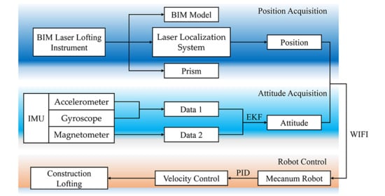
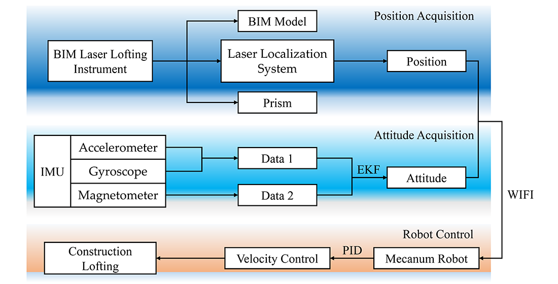
In data acquisition, we discuss the localization and attitude separately which will effectively reduce the amount of estimation and calculation. Figure 1 shows the integration framework;

(3)

We adopt a simple and efficient ground robot motion control theory. It is suitable for Mecanum wheel robots and indoor barrier-free environment;

(4)

We propose a system combining multi-sensors and BIM laser lofting instrument. It expands the relevant market and provides a reference for the future three-dimensional intelligent lofting under multi-scenes.

The paper is organized as follows. Section 2 summarizes the related work of robot localization and lofting environmental adaptability. The design of the robot platform is shown in Section 3. Brief introduction of BIM laser lofting instrument and acquisition of location information are introduced in Section 4. Section 5 presents multi-sensor data fusion for attitude estimation. The theory of robot motion control is described in Section 6. Section 7 shows the experimental results. Section 8 is the discussion of the experimental results. Finally, the conclusion is given in Section 9.

2. Related Work

There are many operating steps in construction lofting, such as setting up instruments, aligning, leveling, locating, and marking, among which locating accurately is a critical step. Therefore, for the robot to reach the control points accurately in a strange environment, it is essential to get the robot’s state.

Many scholars have carried out researches on the localization of robots in a strange environment. The related work mainly includes the requirement of precision, application environment, selecting and combining sensors, and others. Multi-sensors are usually used in these researches to estimate the state information of ground robots or flying robots. GPS-RTK positioning method is mature enough and has high positioning accuracy. Jiang [16] has successfully used GPS technology for the layout of the bridge construction horizontal control network and the bridge axis lofting work, and achieved high enough lofting accuracy. However, this method is commonly used for outdoor navigation or positioning and is not suitable for the indoor environment. Simultaneous localization and mapping (SLAM) technology is currently the main method for robot localization in indoor environment. It can be applied in an indoor environment and can be used for real-time mapping of the environment so that the robots can work in this environment for a long time. Many indoor robots have adopted this technology [17,18]. However, this method usually needs to compare with the dynamic map to reduce the errors. Different construction sites are completely different, therefore, SLAM technology cannot be well applied in lofting. Ultra-wideband (UWB) is also one of the common methods for indoor localization, but its accuracy is not enough [19,20]. IMU as one of the most commonly used sensors for robot state estimation can be seen in almost all current robot localization researches. However, due to the huge accumulative errors caused by wheel slip, sensor drift, and other reasons [21] (pp. 483–484), it can hardly be used alone in high-precision state estimation research. More sensors must be used for position or attitude correction, such as Lidar, camera or magnetometer, etc. Lidar/IMU [22,23,24], camera/IMU [25,26,27], Lidar/Camera/IMU [28,29,30], and other multi-sensor combinations methods can estimate the robot’s state through feature matching algorithms. However, these methods still have problems such as insufficient real-time performance and environmental adaptability. Non-feature or similar features of the lofting environment also makes these methods inapplicable. Although these methods cannot be fully applied to lofting conditions, IMU is still very efficient in estimating robot state at present.

In [31], the author proposed a method of using two GPS-RTK units to fuse IMU data to estimate the vehicle’s three-dimensional attitude, position, and velocity. However, this method cannot solve the robot localization problem in indoor or signal occlusion environment. Liu [32] describes a robot localization method based on laser SLAM, but high-precision laser radar is often costly. To solve this problem, visual slam was proposed. This method can match depth data by using feature matching algorithm [33], but the accuracy of this method needs to be corrected by loop detection which wastes a lot of time. A dim environment will also affect localization. In [34], the author used the EKF algorithm to fuse multi-sensor data including laser SLAM, visual SLAM, IMU, magnetometer, and other sensors to locate the robot. It was verified that the method can be applied to indoor and outdoor environments through many experiments. These methods of fusing multi-sensor data have achieved good results from an unknown location in an unknown environment. However, as for lofting, the robot usually starts from a known point and the first party will provide at least two known points (or a known direction and a known point) and the points to be lofted. Therefore, the points to be lofted can be reached only by solving the relative localization relationship between points. The above-mentioned methods will increase the calculation amount and cost. In [35], the author achieved state estimation by analyzing the kinematic model of the robot and corrected wheel-slippage error to a certain extent. However, this approach, which used IMU and wheel encoder requires very accurate motion estimation and cannot solve the problem of accumulative error fundamentally. The lack of external sensors for position correction will also produce huge accumulative errors after long-time or long-distance operation. Ferreira [36] described the method of integrating sensors inside buildings and BIM to determine the location of people in buildings. Although this is the localization of people, it can be seen that BIM has a guiding significance for indoor localization in some degree. Considering the existing technologies, application scenarios, and the purpose of improving lofting efficiency, this paper focuses on the localization and navigation of ground robots. It is used in the indoor barrier-free plane environment by combining BIM laser lofting instrument, BIM model, wheel encoder, MEME-IMU, and magnetometer. The final experiment shows that the results meet the lofting accuracy requirements of most construction projects.

3. General Design

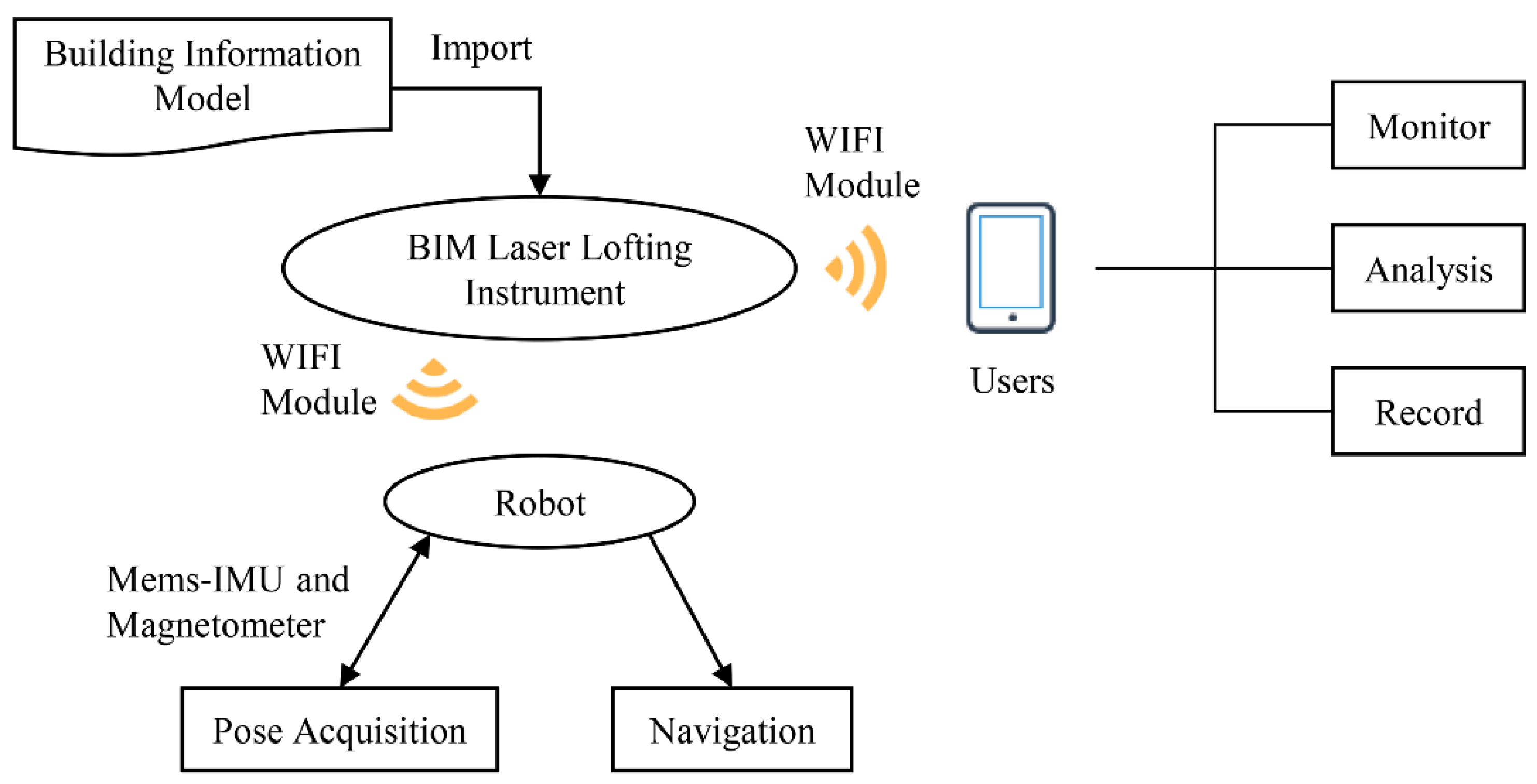
The intelligent lofting system mainly includes three parts: a ground robot, a BIM laser lofting instrument, and a user terminal. Among them, the ground robot moves on the construction site autonomously, communicates with the BIM laser lofting instrument by WIFI module, and processes the data sent by the lofting instrument and multi-sensors. BIM laser lofting instrument gets the robot plane position information in real-time and sends it to the robot and the user terminal through the WIFI module. The user terminal carries out monitoring, manual analysis, and data recording on the construction site according to the feedback information. Figure 2 shows the general structure of the intelligent lofting system. This section mainly introduces the hardware design of the robot.

3.1. Robot Platform Design

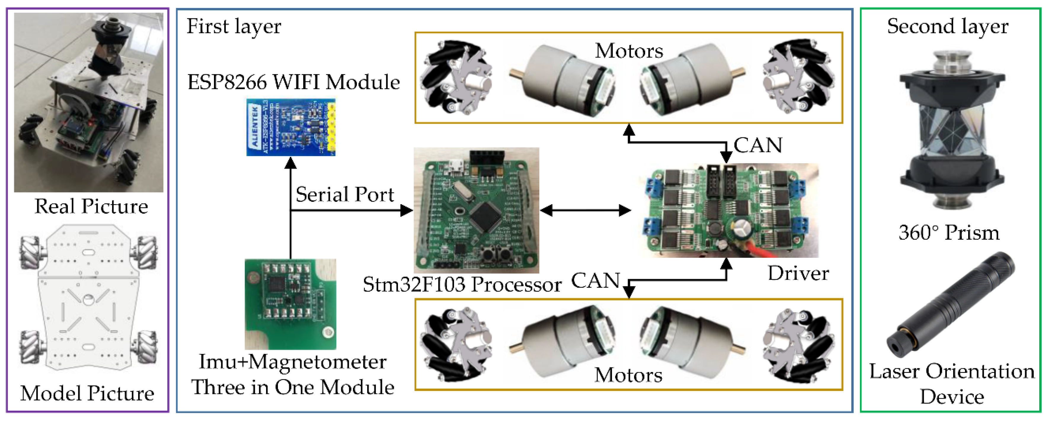
The flexibility and robustness of the ground robot are the basic guarantees for high-precision localization so the size of the robot should not be too large. In this paper, the Mecanum Wheel Chassis of the Home of Balancing Trolley was selected as the chassis of the ground robot, and the secondary development was carried out on it. The chassis of the robot adopted aluminum alloy chassis with a total weight of about 3 KG. The overall size of the chassis was 200 × 250 × 70 mm. We deployed a 7 W DC motor to realize four-wheel drive, and used a 12 V lithium battery with a capacity of 3500 mah as the power supply. We also used the STM32F103 series processor as the control system of the robot, and connected the motor, and drive through the CAN bus. The maximum speed of it was 1.2 m/s, the maximum payload was 6 KG, and the maximum runtime can reach 5 h. In addition, the wheel was matched with an MG513 encoder deceleration motor, which can distinguish rotation of 0.23°.

The BIM laser lofting instrument can obtain the position of the prism on the construction site by linking with the prism through a laser beam. Therefore, the coordinate of the robot on the construction site can be obtained by combining the prism with the robot. To effectively combine the prism with the robot, the ground robot adopted a structure of double-layer. STM32F103 series processor, MEMS-IMU, and magnetometer were installed on the first layer, and a 360° prism and laser orientation device was fixed on the second layer by a customized chassis. This design can ensure the prism to receive laser beams at all angles and will not cause beam occlusion. Figure 3 shows the overall design of the robot.

3.2. Mecanum Wheel

Traditional ground robots usually use rubber wheels as driving wheels, which are low cost, high load-bearing, and durable. However, they are difficult to rotate in the moving, which is not conducive to reaching points in a high-precision way. To solve this problem, the Mecanum wheel with 360° self-rotation characteristic was selected. The Mecanum wheel was invented by the Swedish engineer Bengt Ilon [37], and it can translate and rotate in any direction in the plane through the interaction among a plurality of wheels. This section introduces the mechanical analysis of a single Mecanum wheel and the feasibility of self-rotation.

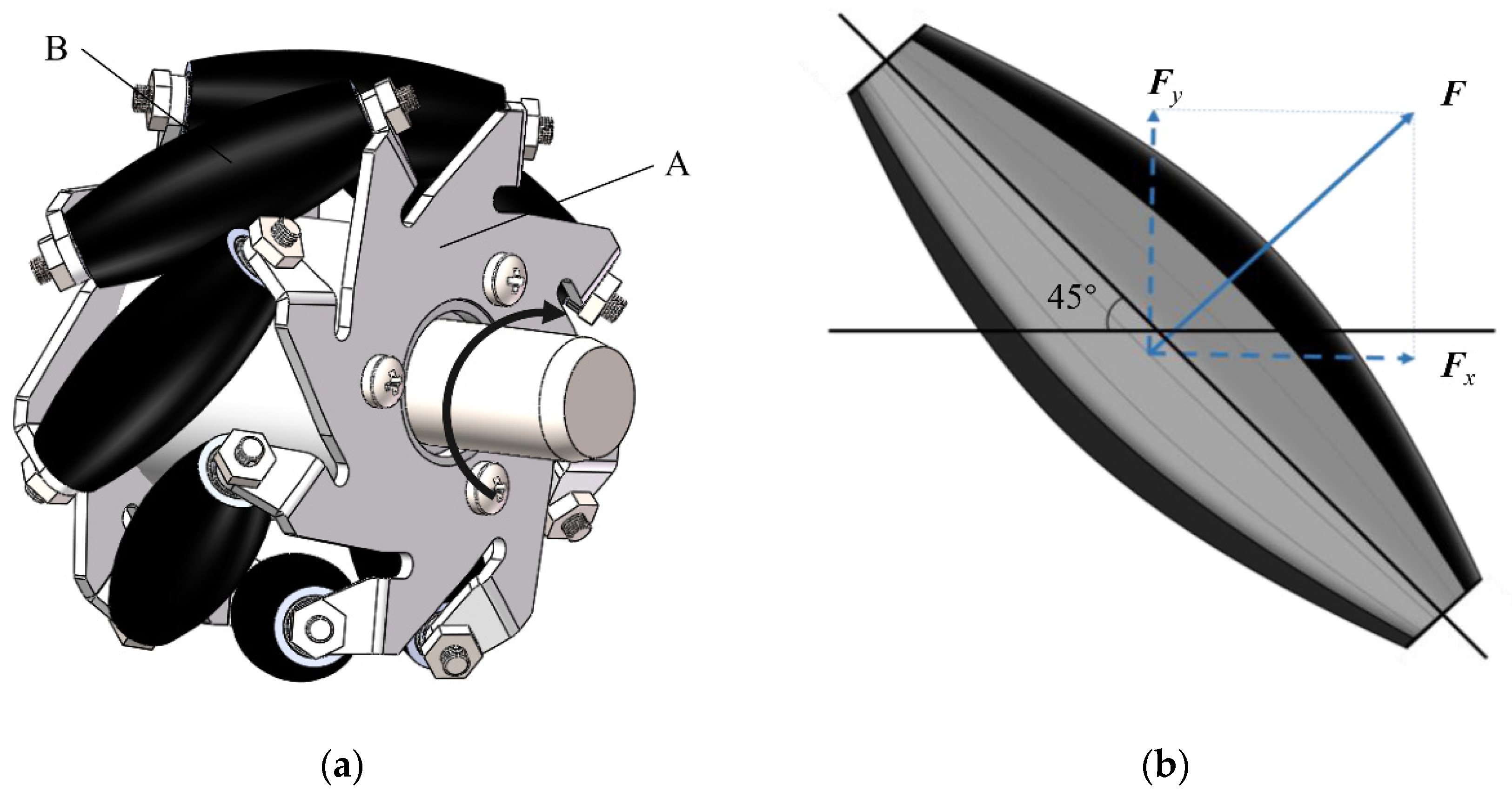
Figure 4a is the structural diagram of the Mecanum wheel, which mainly comprises a hub A and wheel roller B. A is the main support of the whole wheel, and B is a drum mounted on the hub. The angle between A and B is usually ±45°.

Figure 4b shows the force model of the bottom wheel. When the motor drives the wheel to rotate clockwise, friction force F perpendicular to the centerline of the roller is generated. F can be decomposed into a lateral direction force F_x and a longitudinal direction force F_y as shown by the dotted line. It can be seen that unlike a conventional rubber wheel, the Mecanum wheel generates an extra component force F_x perpendicular to the forward direction.

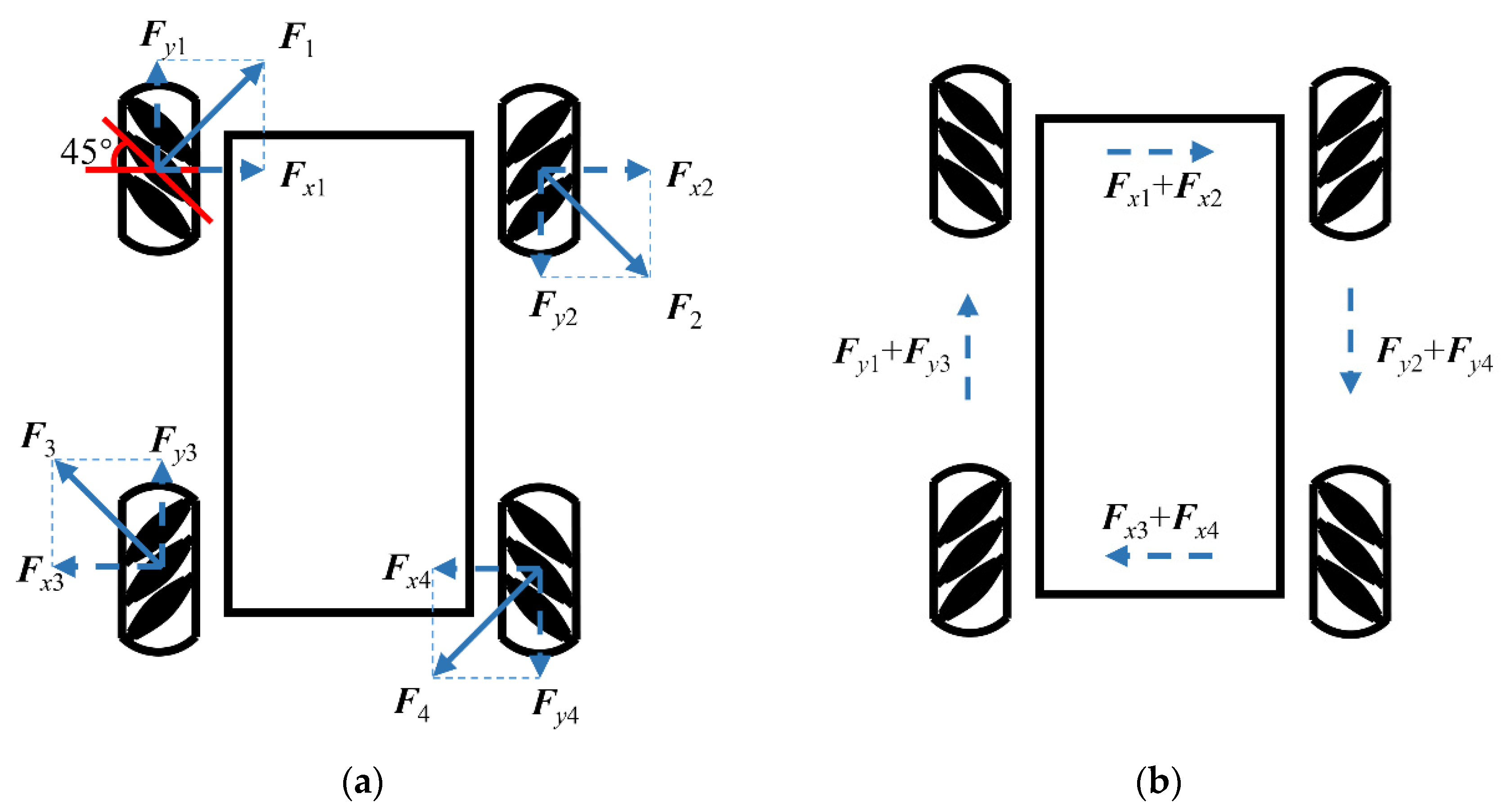
According to the above-mentioned characteristics of the Mecanum wheel, the robot can self-rotate 360° through the cooperation of multiple wheels. In our system, there were four Mecanum wheels and each wheel equipped a separate motor drive. As shown in Figure 5a, to verify the feasibility of self-rotation, taking the clockwise rotation of the robot as an example. When the wheels 1, 2, 3, and 4 rotate clockwise at the same velocity, they generate friction forces F₁, F₂, F₃ and F₄ perpendicular to the centerline of the wheel roller, and the forces are decomposed:

$${\overrightarrow{\mathit{F}}}_i={\overrightarrow{\mathit{F}}}_{xi}+{\overrightarrow{\mathit{F}}}_{yi}(i=1,2,3,4)$$

(1)

where F_xi is the lateral component of force F_i; F_yi is the longitudinal component of force F_i.

Due to the interaction between the forces, the force model can be simplified to Figure 5b, of which, the angle between the hub axis and roller axis is 45°, so F_xi = F_yi(i = 1,2,3,4). Taking F_x1 + F_x2 and F_x3 + F_x4 as an example, the two parallel forces are the same in magnitude and opposite in direction, so the generated force couple will make the robot produce a pure rotation effect and make it rotate. The cooperation of the four Mecanum wheels can provide the robot with 3 degrees of freedom necessary for the omnidirectional rotation in the horizontal plane.

3.3. Inverse Kinematic Analysis

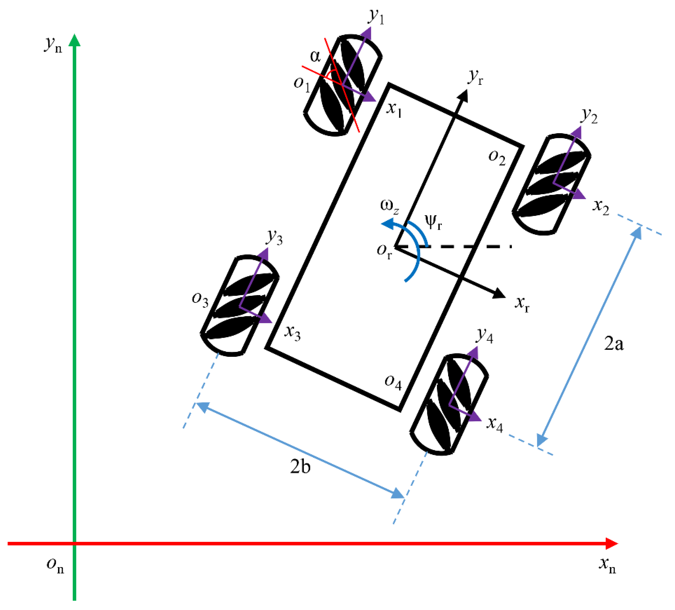
The velocity control of the robot can ensure that it operates stably and efficiently. Figure 6 shows the inverse kinematics analysis of the Mecanum wheel robot. The robot was equipped with four wheels symmetrically, wherein the angle α = 45° in our system. When the robot is placed on the ground horizontally, the position and the angle corresponding to the center point o_r of the robot are taken as state variables. The vehicle coordinate system ∑o_r is established based on point o_r, which is also the placement point of the prism.

At this time, the state of the robot in the vehicle coordinate system ∑o_r is ${\mathit{P}}_{\mathrm{r}}={[\begin{array}{ccc}{x}_{\mathrm{r}}& y_{\mathrm{r}}& {\psi }_{\mathrm{r}}\end{array}]}^{\mathrm{T}}$, and the kinematic formula of each wheel is expressed as:

$$\{\begin{array}{l}{V}_x^{(\mathrm{r})}=(V_1-V_2-V_3+V_4)/4\hfill \\ V_y^{(\mathrm{r})}=(V_1+V_2+V_3+V_4)/4\hfill \\ {\omega }_z^{(\mathrm{r})}=(-V_1+V_2-V_3+V_4)/4\ast (a+b)\hfill \end{array}$$

(2)

where $V_x^{(\mathrm{r})}$ is the lateral velocity component in the vehicle coordinate system, with the right as positive, $V_y^{(\mathrm{r})}$ is the longitudinal velocity component in the vehicle coordinate system, with the upward as positive, ${\omega }_z^{(\mathrm{r})}$ is the angular velocity around the center of the car body, with counterclockwise as positive, V_i (i = 1, 2, 3, 4) is the linear velocity of wheel i, a is half the length of the car, b is half the width of the car.

And the velocity of the robot in the navigation coordinate system ∑o_n is:

$${\mathit{V}}^{(\mathrm{n})}=\left[\begin{array}{c}{V}_x^{(\mathrm{n})}\\ V_y^{(\mathrm{n})}\\ {\omega }_z^{(\mathrm{n})}\end{array}\right]=\mathit{R}({\psi }_{\mathrm{r}}){\mathit{V}}^{(\mathrm{r})}=\left[\begin{array}{ccc}\cos {\psi }_{\mathrm{r}}& -\sin {\psi }_{\mathrm{r}}& 0\\ \sin {\psi }_{\mathrm{r}}& \cos {\psi }_{\mathrm{r}}& 0\\ 0& 0& 1\end{array}\right]\left[\begin{array}{c}{V}_x^{(\mathrm{r})}\\ V_y^{(\mathrm{r})}\\ {\omega }_z^{(\mathrm{r})}\end{array}\right]$$

(3)

where V⁽ⁿ⁾ is the horizontal velocity component, vertical velocity component, and angular velocity of the robot in the ∑o_n, $\mathit{R}({\psi }_{\mathrm{r}})$ is the transformation matrix from ∑o_r to ∑o_n.

The velocity of each wheel in the navigation coordinate system can be obtained from Equations (2) and (3):

$$\left[\begin{array}{c}{V}_1\\ V_2\\ V_3\\ V_4\end{array}\right]=\left[\begin{array}{ccc}\cos {\psi }_{\mathrm{r}}-\sin {\psi }_{\mathrm{r}}& \cos {\psi }_{\mathrm{r}}+\sin {\psi }_{\mathrm{r}}& -(\mathrm{a}+\mathrm{b})\\ -(\cos {\psi }_{\mathrm{r}}+\sin {\psi }_{\mathrm{r}})& \cos {\psi }_{\mathrm{r}}-\sin {\psi }_{\mathrm{r}}& \mathrm{a}+\mathrm{b}\\ -(\cos {\psi }_{\mathrm{r}}+\sin {\psi }_{\mathrm{r}})& \cos {\psi }_{\mathrm{r}}-\sin {\psi }_{\mathrm{r}}& -(\mathrm{a}+\mathrm{b})\\ \cos {\psi }_{\mathrm{r}}-\sin {\psi }_{\mathrm{r}}& \cos {\psi }_{\mathrm{r}}+\sin {\psi }_{\mathrm{r}}& \mathrm{a}+\mathrm{b}\end{array}\right]\left[\begin{array}{c}{V}_x^{(\mathrm{n})}\\ V_y^{(\mathrm{n})}\\ {\omega }_z^{(\mathrm{n})}\end{array}\right]$$

(4)

Although the velocity of the real motion model of the robot is calculated, the velocity of the wheels lags behind due to friction and other reasons during actual running. Direct velocity calculation is difficult to keep the car stable, therefore, this paper uses wheel encoders and PID control to set the velocities:

$$V=k_p{e}_v+k_i{\displaystyle \int e_v}+k_d\stackrel{•}{e_v}$$

(5)

where k_p is the proportional coefficient, k_i is the integral coefficient, k_d is the differential coefficient, $e_v=V_i-V_i^{(real)}(i=1,2,3,4)$, $V_i^{(real)}$ is the real velocity of wheels which can be obtained from wheel encoder feedback.

To verify the stability of the velocity control, a set of experiments was carried out. We commanded the robot to reach the designated position (10, 0) from the origin (0, 0) in a straight line, with a total length of 10 m and 10 times experiments. The experimental results are shown in

Table 1. The results of speed control experiment.

Experiments	Starting Position/m	Expected Position/m	Actual Position/m	Error/mm
1	(0, 0)	(10, 0)	9.990	10
2	(0, 0)	(10, 0)	9.996	4
3	(0, 0)	(10, 0)	9.991	9
4	(0, 0)	(10, 0)	9.993	7
5	(0, 0)	(10, 0)	9.993	7
6	(0, 0)	(10, 0)	9.992	8
7	(0, 0)	(10, 0)	9.993	7
8	(0, 0)	(10, 0)	9.997	3
9	(0, 0)	(10, 0)	9.990	10
10	(0, 0)	(10, 0)	9.992	8

:

It can be seen from Table 1 that the maximum error is 10 mm, the Root Mean Squared Error (RMSE) is 2.1932 mm.

4. BIM Laser Lofting Instrument

In this paper, we use a BIM laser lofting instrument and 360° prism to get the high-precision position of the robot. BIM laser lofting instrument refers to a new generation of lofting instrument that combines BIM and laser dynamic beam orientation system. The instrument is easy to operate, and can be automatically leveled or manually leveled with one key after startup. “What we see is what we get” on the construction site is realized through highly visible guiding light, and each point is lofted independently without cumulative errors. Users can use the Personal Digital Assistant (PDA) to monitor the position of the prism in real-time and move it to the points to be lofted according to instructions, with the maximum lofting distance is up to 100 m and measuring accuracy is ±3 mm (Distance)/5″ (Angle). We selected the BIM laser lofting instrument of Topcon LN-100 to carry out our experiment. Figure 7a shows the introduction of the instrument, and Figure 7b is a 360° prism used together.

Table 2. The main parameters of Topcon LN-100.

LN-100	Parameters
Measuring accuracy	±3 mm (Distance)/5″ (Angle)
Laser tracking range	0.9–100 m
Working range	360° (Horizontal), ±25°(Vertical)
Leveling range	±3°
Wireless LAN	802.11 n/b/g
Communication range	100 m

shows the main parameters of the Topcon LN-100.

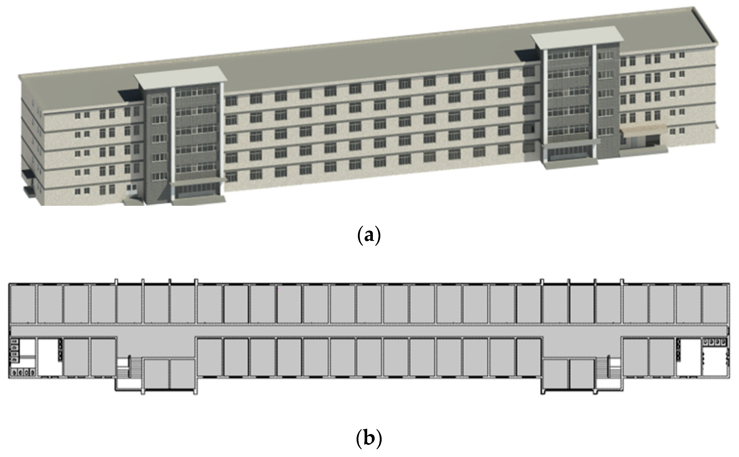
Among them, BIM mentioned above refers to a digital model with geometric information, state information, and professional attributes of building construction. In the process of lofting, the model mainly provides an independent coordinate system, known points, and position of points to be lofted. Users can intuitively observe the position relationship between prism and points to be lofted through the model. Figure 8 is a BIM of a teaching building in Tongji University built by Autodesk Revit, where Figure 8a is the overall appearance of the building model, and Figure 8b is the first floor of the building.

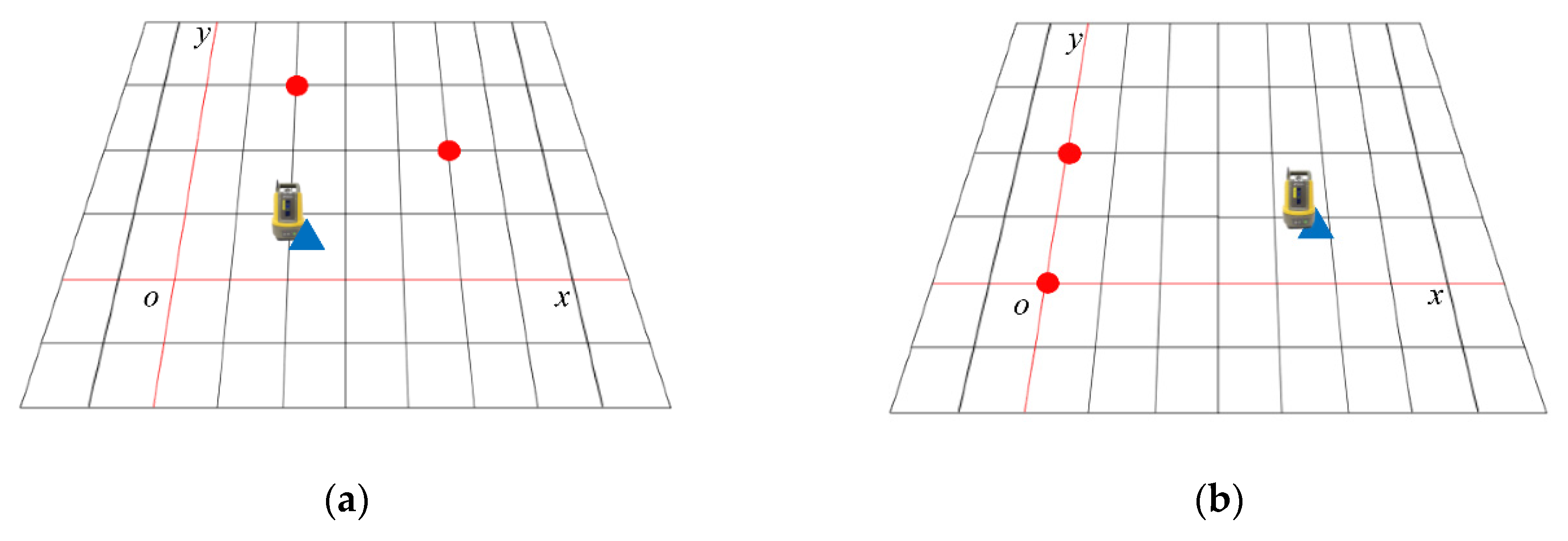
This instrument provides four station layout methods, which are applicable to almost all lofting construction environment. The four methods are, respectively, Resection method, Reference Axis (Base Point and Reference Axis) Measurement method, Backsight Point (Known Point) Measurement method, and Backsight Point (Reference Axis on the Base Point) Measurement method. Figure 9 is a schematic diagram of the four station setting methods, in which red points represent known positions, and blue triangles represent random positions:

• Resection: the instrument is set up arbitrarily and measure two or more known points to establish a coordinate system;
• Reference Axis (Base Point and Reference Axis) Measurement: the instrument is set up arbitrarily and measure the base point (0,0) and the point on the reference axis (x axis or y axis) to establish a coordinate system;
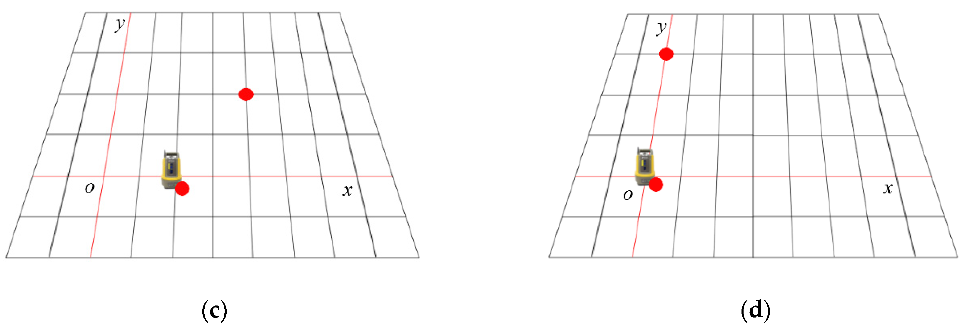
• Backsight Point (Known Point) Measurement: position the instrument on a known point, measure another known point to establish a coordinate system;
• Backsight Point (Reference Axis on the Base Point) Measurement: position the instrument on the base point (0,0), measure the point on the reference axis (x axis or y axis) to establish a coordinate system.

In our experiment, the 360° prism was fixed at the geometric center of the robot. The robot and Topcon LN-100 are connected via the WIFI communication module and Transmission Control Protocol (TCP). The position (x,y) of the prism received by the WIFI module was sent to the processor in real-time, wherein, the data transmission frequency is 20 Hz and the maximum communication distance can reach 100 m.

5. Multi-Sensors Fusion Algorithm

For the attitude estimation of the ground robot, it is usually output by multi-sensors. We use MEMS-IMU and magnetometer to get the attitude of the ground robot. Among them, magnetometer and accelerometer in MEMS-IMU output one group of robot attitude, and gyroscope in MEMS-IMU output another group of robot attitude. However, due to the defects and accumulative errors of a single sensor, neither of the two groups of estimations can be used as the attitude of the robot for a long time alone. Therefore, the EKF algorithm is adopted to fuse the two groups of data for optimal estimation of robot attitude. This part will introduce the EKF algorithm fusing multi-sensor data.

5.1. Sensors Angle Output

The common attitude measurement sensors cannot directly obtain angle data. For example, the data output by the gyroscope is usually the angular velocity of the robot and must be converted into angle through integration. This part briefly analyzes the conversion process of accelerometer, magnetometer, and gyroscope:

5.1.1. Accelerometer

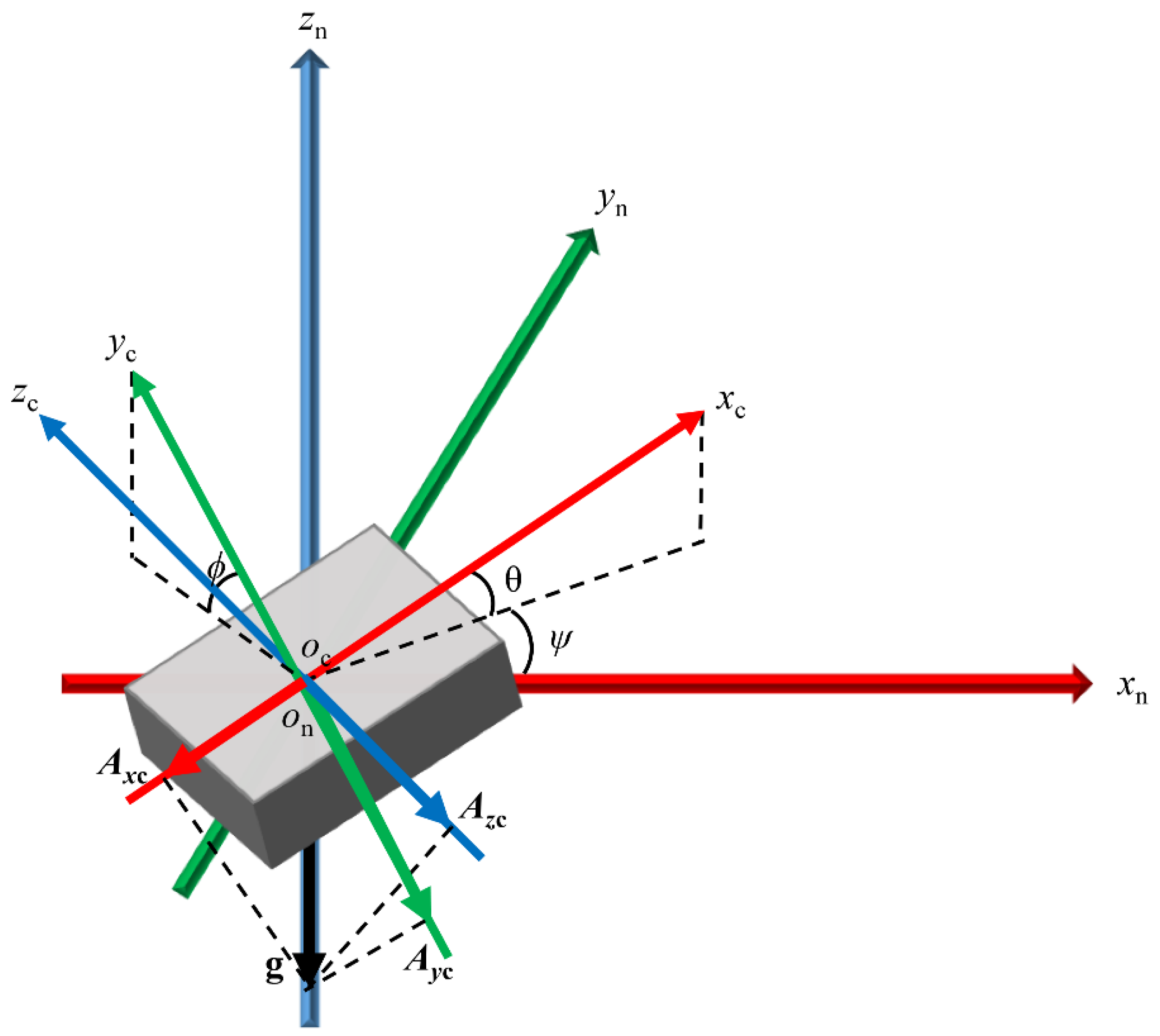
The accelerometer can further get the attitude of the object by collecting acceleration components of gravity acceleration on each axis of the object. The navigation coordinate system in this paper is set as the east (x) north (y) sky (z) coordinate system. As shown in Figure 10, a calibrated accelerometer T_a is obliquely placed in space, its rotation process is $\mathit{R}(\mathbf{·})=\mathit{X}(\mathbf{·})\mathit{Y}(\mathbf{·})\mathit{Z}(\mathbf{·})$, and assumes that it rotates all in the positive direction of the attitude angle. It finally outputs the projection component ${\mathit{A}}_{\mathrm{c}}={\left[\begin{array}{ccc}{A}_x^{(\mathrm{c})}& A_y^{(\mathrm{c})}& A_z^{(\mathrm{c})}\end{array}\right]}^{\mathrm{T}}$ of the gravity acceleration g on the three axis x_c, y_c, z_c of the carrier coordinate system ∑o_c.

The rotation matrix is calculated as follows:

$$\begin{array}{ll}\left[\begin{array}{c}{A}_x^{(\mathrm{c})}\\ A_y^{(\mathrm{c})}\\ A_z^{(\mathrm{c})}\end{array}\right]& =\mathit{R}(\mathbf{·})\left[\begin{array}{c}0\\ 0\\ \mathrm{g}\end{array}\right]=\mathit{X}(\mathbf{·})\mathit{Y}(\mathbf{·})\mathit{Z}(\mathbf{·})\left[\begin{array}{c}0\\ 0\\ \mathrm{g}\end{array}\right]\\ & =\left[\begin{array}{ccc}1& 0& 0\\ 0& \cos \phi & \sin \phi \\ 0& -\sin \phi & \cos \phi \end{array}\right]\left[\begin{array}{ccc}\cos \theta & 0& -\sin \theta \\ 0& 1& 0\\ \sin \theta & 0& \cos \theta \end{array}\right]\left[\begin{array}{ccc}\cos \psi & \sin \psi & 0\\ -\sin \psi & \cos \psi & 0\\ 0& 0& 1\end{array}\right]\left[\begin{array}{c}0\\ 0\\ \mathrm{g}\end{array}\right]\\ & =\left[\begin{array}{c}-\mathrm{g}\sin \theta \\ \mathrm{g}\sin \phi \cos \theta \\ \mathrm{g}\cos \phi \cos \theta \end{array}\right]\end{array}$$

(6)

where g is the gravity acceleration, taking g = 9.8 m/s², $\mathit{R}(\mathbf{·})$ is the rotation matrix, ${\mathit{A}}_{\mathrm{c}}={\left[\begin{array}{ccc}{A}_x^{(\mathrm{c})}& A_y^{(\mathrm{c})}& A_z^{(\mathrm{c})}\end{array}\right]}^{\mathrm{T}}$ is the components of the gravitational acceleration on the three-axis of the carrier coordinate system ∑o_c, φ, θ and ψ is the Roll angle, Pitch angle, and Yaw angle of accelerometer T_a in ∑o_c.

According to Equation (6), the converted angle of the data collected by the accelerometer is:

$$\{\begin{array}{c}\theta =\arcsin (-A_x^{(\mathrm{c})}/\mathrm{g})\\ \phi =\arctan (A_y^{(\mathrm{c})}/A_z^{(\mathrm{c})})\end{array}$$

(7)

5.1.2. Magnetometer

The magnetometer can get the magnetic field intensity components on each axis of the object, and then calculate the Yaw angle ψ. Its conversion principle is similar to the accelerometer, so it will not be illustrated here with a figure. First, without considering the magnetic declination, assume that a calibrated magnetometer T_m is obliquely placed on the ground. Then, T_m outputs the magnetic field intensity components ${\mathit{M}}_{\mathrm{c}}={\left[\begin{array}{ccc}{M}_x^{(\mathrm{c})}& M_y^{(\mathrm{c})}& M_z^{(\mathrm{c})}\end{array}\right]}^T$ of the earth’s magnetic field H on the three axis x_c, y_c, z_c of the carrier coordinate system ∑o_c. Finally, the Yaw angle ψ can be calculated as follows:

$$\psi =\arctan (M_y^{(\mathrm{c})}/M_x^{(\mathrm{c})})$$

(8)

However, in the actual running of the robot, it is impossible to keep a constant plane motion. The unevenness of the road surface and the ground gap will cause the robot to generate an instantaneous Pitch angle or Roll angle. Due to the influence of Pitch and Roll, Equation (8) is no longer valid. Therefore, without considering the magnetic declination, assume that magnetometer T_m is placed obliquely in space and its rotation matrix is $\mathit{R}(\mathbf{·})=\mathit{X}(\mathbf{·})\mathit{Y}(\mathbf{·})\mathit{Z}(\mathbf{·})$, all rotation in the positive direction of the attitude angle. Then the rotation matrix can be calculated as follows:

$$\begin{array}{ll}\left[\begin{array}{c}{M}_x^{(\mathrm{c})}\\ M_y^{(\mathrm{c})}\\ M_z^{(\mathrm{c})}\end{array}\right]& =\mathit{R}(\mathbf{·})\left[\begin{array}{c}0\\ H_y\\ H_z\end{array}\right]=\mathit{X}(\mathbf{·})\mathit{Y}(\mathbf{·})\mathit{Z}(\mathbf{·})\left[\begin{array}{c}0\\ H_y\\ H_z\end{array}\right]\\ & =\left[\begin{array}{c}\cos \theta \sin \psi H_y-\sin \theta H_z\\ (\sin \phi \sin \theta \sin \psi +\cos \phi \cos \psi )H_y+\sin \phi \cos \theta H_z\\ (\cos \phi \sin \theta \sin \psi +\sin \phi \cos \psi )H_y+\cos \phi \cos \theta H_z\end{array}\right]\end{array}$$

(9)

where the Pitch angle θ and Roll angle ψ are known from Equation (7), $\mathit{H}={\left[\begin{array}{ccc}0& H_y& H_z\end{array}\right]}^{\mathrm{T}}$ is the magnetic field intensity of point o_c in the earth’s magnetic field coordinate system, and H_x = 0 because the geomagnetic direction is from the geomagnetic south pole to the geomagnetic north pole, ${\mathit{M}}_c={\left[\begin{array}{ccc}{M}_x^{(\mathrm{c})}& M_y^{(\mathrm{c})}& M_z^{(\mathrm{c})}\end{array}\right]}^{\mathrm{T}}$ is the component of the earth’s magnetic field on the three-axis of the carrier coordinate system ∑o_c.

Simultaneous Equations (7) and (9) can get the Yaw angle $\psi$ as follows:

$$\psi =\arctan (\frac{M_x^{(\mathrm{c})}\cos \theta +M_y^{(\mathrm{c})}\sin \theta \sin \phi +M_z^{(\mathrm{c})}\sin \theta \cos \phi }{\cos \phi M_y^{(\mathrm{c})}-\sin \phi M_z^{(\mathrm{c})}})$$

(10)

The Yaw angle ψ obtained by magnetometer, Pitch angle θ, and Roll angle φ obtained by acceleration are fused with gyroscope data as a group of attitude.

5.1.3. Gyroscope

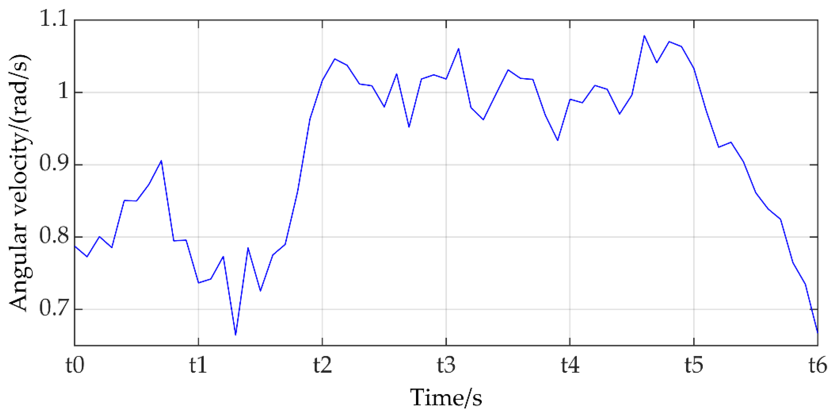
The gyroscope collects angular velocity ${\omega }_i(i=x,y,z)$ of each axis when the object rotates and further gets the attitude of the object through integration with time.

As shown in Figure 11, taking the Pitch angle as an example. Assuming that the gyroscope’s Pitch angle at time $t_0$ is ${\theta }_0$, at time $t_1$ is ${\theta }_1$, and its angular velocity during this period is a function ${\omega }_y(t)$, then:

$${\theta }_1={\theta }_0+{\displaystyle \underset{t_0}{\overset{t_1}{\int }}{\omega }_y(t)dt}$$

(11)

where ${\omega }_y(t)$ is the relationship between angular velocity on the axis $y$ and time $t$.

The calculation of the $\phi$ Roll angle and the Yaw angle $\psi$ is the same as above, namely:

$$\{\begin{array}{c}{\phi }_1={\phi }_0+{\displaystyle \underset{t_0}{\overset{t_1}{\int }}{\omega }_x(t)dt}\\ {\psi }_1={\psi }_0+{\displaystyle \underset{t_0}{\overset{t_1}{\int }}{\omega }_z(t)dt}\end{array}$$

(12)

Pitch angle $\theta$, Roll angle $\phi$, and Yaw angle $\psi$ obtained by the gyroscope are fused with accelerometer and magnetometer data as another group of attitudes.

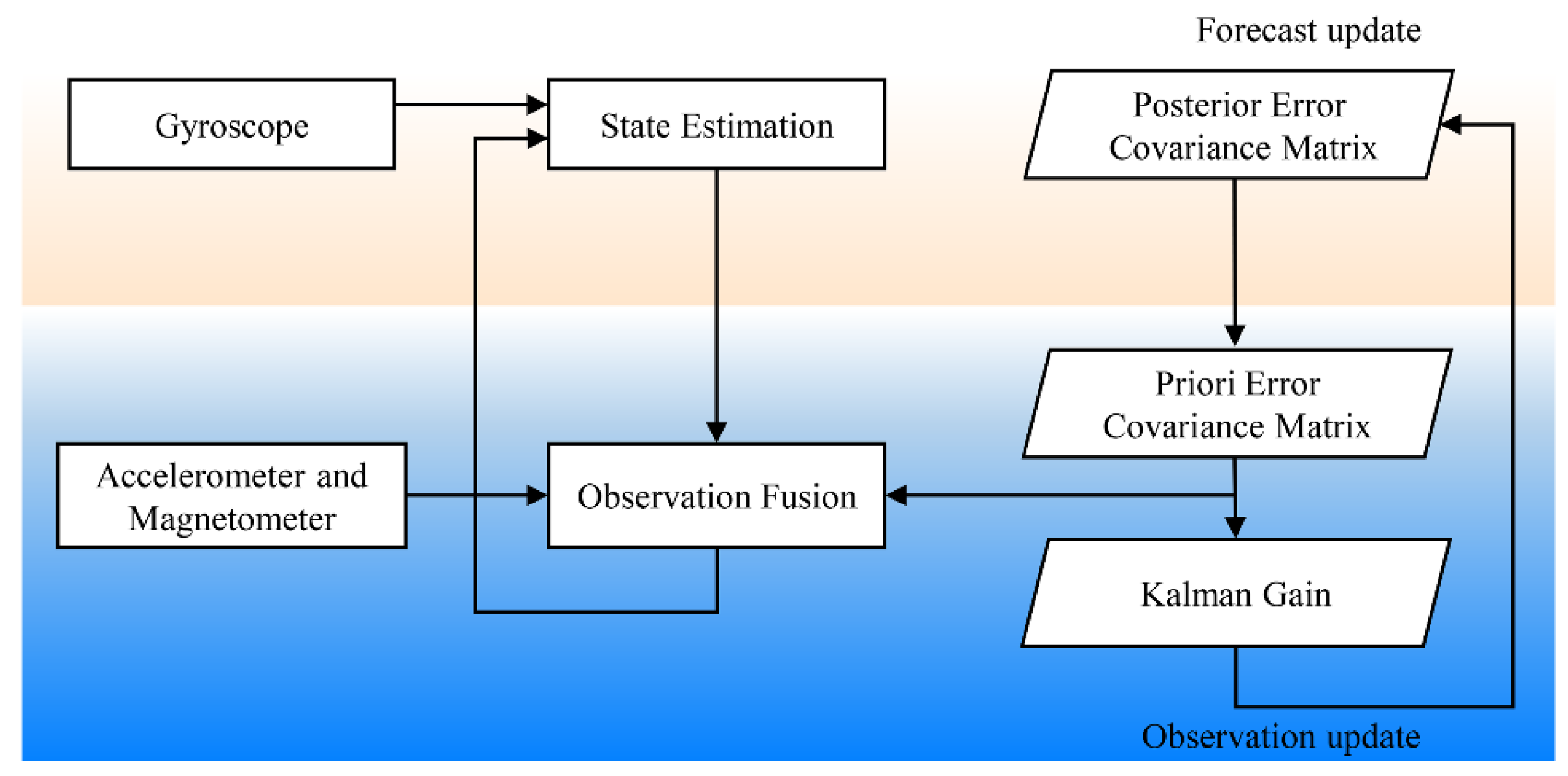
5.2. Data Fusion Algorithm

Kalman filter is one of the most efficient algorithms to fuse multi-sensor data when estimating the state of a robot at present. This algorithm continuously optimizes the state of the system by inputting observation data and outputs the optimal estimation of the state of the system. However, this algorithm is generally applicable to linear systems and is not applicable to the robot system in this paper. Considering the nonlinear characteristics of the system and the high efficiency of the fusion algorithm, we adopted the EKF algorithm for multi-sensor data fusion of nonlinear systems.

Extended Kalman Filter

In this study, the sensors were directly fixed to the robot and have been pre-calibrated. The state equation of the system is expressed as:

$${\mathit{x}}_k=f({\mathit{x}}_{k-1},{\mathit{u}}_{k-1},{\mathit{w}}_{k-1})=\left[\begin{array}{cc}{(\mathit{I}+\frac{T}{2}\mathit{\gamma }({\mathit{w}}_{ik}))}_{4\times 4}& {\mathbf{0}}_{4\times 3}\\ {\mathbf{0}}_{3\times 4}& {\mathit{I}}_{3\times 3}\end{array}\right]{\mathit{x}}_{k-1}+{\mathit{w}}_{k-1}$$

(13)

where regardless of the input variables of the system, ${\mathit{u}}_{k-1}=0$, ${\mathit{x}}_k$ is state variable, $T$ is the update time, $\frac{1}{2}\mathit{\gamma }({\mathit{w}}_{ik})$ is a quaternion differential equation expression, ${\mathit{w}}_{k-1}$ is process noise, which follows Gaussian distribution with a mean value of 0, namely ${\mathit{w}}_k~N(0,Q)$.

The state variable is selected as:

$${\mathit{x}}_k={\left[\begin{array}{ccccccc}{q}_{\omega }& q_x& q_y& q_z& w_{xk}^{(\mathrm{g})}& w_{yk}^{(\mathrm{g})}& w_{zk}^{(\mathrm{g})}\end{array}\right]}^{\mathrm{T}}$$

(14)

where $\mathit{q}={\left[\begin{array}{cccc}{q}_{\omega }& q_x& q_y& q_z\end{array}\right]}^{\mathrm{T}}$ is a quaternion in the world coordinate system to represent the robot’s attitude, ${\mathit{w}}_{ik}^{(\mathrm{g})}(i=x,y,z)$ represents gyro drift deviation on the axis $i$ at time k.

$\mathit{\gamma }({\mathit{w}}_{ik})$ is expressed as:

$$\mathit{\gamma }({\mathit{w}}_{ik})=\left[\begin{array}{cccc}0& -({\omega }_{xk}-w_{xk}^{(\mathrm{g})})& -({\omega }_{yk}-w_{yk}^{(\mathrm{g})})& -({\omega }_{zk}-w_{zk}^{(\mathrm{g})})\\ {\omega }_{xk}-w_{xk}^{(\mathrm{g})}& 0& {\omega }_{zk}-w_{zk}^{(\mathrm{g})}& -({\omega }_{yk}-w_{yk}^{(\mathrm{g})})\\ {\omega }_{yk}-w_{yk}^{(\mathrm{g})}& -({\omega }_{zk}-w_{zk}^{(\mathrm{g})})& 0& {\omega }_{xk}-w_{xk}^{(\mathrm{g})}\\ {\omega }_{zk}-w_{zk}^{(\mathrm{g})}& {\omega }_{yk}-w_{yk}^{(\mathrm{g})}& -({\omega }_{xk}-w_{xk}^{(\mathrm{g})})& 0\end{array}\right]$$

(15)

where ${\mathit{\omega }}_{ik}(i=x,y,z)$ represents the angular velocity on the axis $i$ at time k, which can be got from gyroscope.

The observation equation of the system is expressed as:

$${\mathit{z}}_k=h({\mathit{x}}_k,{\mathit{v}}_k)=\left[\begin{array}{cc}{\mathit{R}}_{3\times 3}^{(\mathrm{n})}& {\mathbf{0}}_{3\times 3}\\ {\mathbf{0}}_{3\times 3}& {\mathit{R}}_{3\times 3}^{(\mathrm{n})}\end{array}\right]\left[\begin{array}{c}0\\ 0\\ -\mathrm{g}\\ 0\\ H_y\\ H_z\end{array}\right]+v_k=\left[\begin{array}{c}{\mathit{h}}_1^{\mathrm{a}}\\ {\mathit{h}}_2^{\mathrm{m}}\end{array}\right]+v_k$$

(16)

where ${\mathit{z}}_k$ is the observation variable, and the accelerometer and magnetometer data are used for the observation, ${\mathit{R}}_{3\times 3}^{(\mathrm{n})}$ is rotation matrix represented by quaternions, $\mathrm{g}$ is gravity acceleration, $H_y$ and $H_z$ refers to the north geomagnetic component and the vertical geomagnetic component of the navigation coordinate system ∑o_n, ${\mathit{h}}_1^{\mathrm{a}}$ is the observation equation of accelerometer, ${\mathit{h}}_2^{\mathrm{m}}$ is the observation equation of magnetometer, ${\mathit{v}}_k$ is observation noise, which follows Gaussian distribution with a mean value of 0, namely ${\mathit{v}}_k~N(0,R)$.

From Equations (13) and (16), it can be seen that functions $f(\mathbf{·})$ and $h(\mathbf{·})$ are nonlinear and need to be linearized. EKF gets state transition matrices ${\mathit{F}}_k$ and ${\mathit{H}}_k$ by solving partial derivatives of nonlinear functions, that is Jacobi matrices:

$${\mathit{F}}_k={\frac{\partial f}{\partial {\mathit{x}}_k}|}_{x={\widehat{x}}_{k-1}}=\left[\begin{array}{cc}{(\mathit{I}+\frac{T}{2}\mathit{\gamma }({\mathit{w}}_k))}_{4\times 4}& {\mathit{\delta }}_{4\times 3}^1\\ {\mathbf{0}}_{3\times 4}& {\mathit{I}}_{3\times 3}\end{array}\right]$$

(17)

$${\mathit{H}}_k={\frac{\partial h}{\partial {\mathit{x}}_k}|}_{x={\widehat{x}}_k}=2\left[\begin{array}{cc}{\delta }_{3\times 4}^2& 0_{3\times 3}\\ {\delta }_{3\times 4}^3& 0_{3\times 3}\end{array}\right]$$

(18)

where, ${\widehat{\mathit{x}}}_k$ is the estimation of ${\mathit{x}}_k$, ${\mathit{\delta }}^1$ is the partial derivative of $f(\mathbf{·})$ to ${\mathit{\omega }}_{ik}$, and the expression is:

$${\mathit{\delta }}^1=\frac{\partial f}{\partial {\mathit{w}}_{ik}}=\frac{T}{2}\left[\begin{array}{ccc}{q}_x& q_y& q_z\\ -q_{\omega }& q_z& -q_y\\ -q_z& -q_{\omega }& q_x\\ q_y& -q_x& -q_{\omega }\end{array}\right]$$

(19)

${\mathit{\delta }}^2$ is the partial derivative of ${\mathit{h}}_1^{\mathrm{a}}$ to $\mathit{q}$, and the expression is:

$${\delta }^2=\frac{\partial {\mathit{h}}_1^{\mathrm{a}}}{\partial \mathit{q}}=\left|\mathrm{g}\right|\left[\begin{array}{cccc}{q}_y& -q_z& q_{\omega }& -q_x\\ -q_x& -q_{\omega }& -q_z& -q_y\\ -q_{\omega }& q_x& q_y& -q_z\end{array}\right]$$

(20)

${\mathit{\delta }}^3$ is the partial derivative of ${\mathit{h}}_2^{\mathrm{m}}$ to $\mathit{q}$, and the expression is:

$${\mathit{\delta }}^3=\frac{\partial {\mathit{h}}_2^{\mathrm{m}}}{\partial \mathit{q}}=\left[\begin{array}{cccc}{H}_y{q}_z+H_z{q}_y& H_y{q}_y-H_z{q}_z& H_y{q}_x+H_z{q}_{\omega }& H_y{q}_{\omega }-H_z{q}_x\\ H_y{q}_{\omega }-H_z{q}_x& -H_y{q}_x-H_z{q}_{\omega }& H_y{q}_y-H_z{q}_z& -H_y{q}_z-H_z{q}_y\\ -H_y{q}_x-H_z{q}_{\omega }& -H_y{q}_{\omega }+H_z{q}_x& H_y{q}_z+H_z{q}_y& H_y{q}_y-H_z{q}_z\end{array}\right]$$

(21)

Finally, the state update equation is obtained:

$${\widehat{\mathit{x}}}_k={\widehat{\mathit{x}}}_k^{-}+{\mathit{K}}_k({\mathit{z}}_k-\mathit{h}({\widehat{\mathit{x}}}_k^{-},0))$$

(22)

where ${\widehat{\mathit{x}}}_k^{-}$ is the prior estimation of ${\mathit{x}}_k$, ${\mathit{K}}_k$ is the Kalman gain, and the expressions of ${\widehat{\mathit{x}}}_k^{-}$ and ${\mathit{K}}_k$ are as follows:

$${\widehat{\mathit{x}}}_k^{-}={\mathit{F}}_k{\widehat{\mathit{x}}}_{k-1}^{-}$$

(23)

$${\mathit{K}}_k={\mathit{P}}_k^{-}{\mathit{H}}_k^{\mathrm{T}}{({\mathit{H}}_k{\mathit{P}}_k^{-}{\mathit{H}}_k^{\mathrm{T}}+\mathit{R})}^{-1}$$

(24)

In Equation (24), ${\mathit{P}}_k^{-}$ is the error covariance matrix of prior estimation at time k, the expression is as follows:

$${\mathit{P}}_k^{-}={\mathit{F}}_k{\mathit{P}}_{k-1}{\mathit{F}}_{k-1}^{\mathrm{T}}+\mathit{Q}$$

(25)

where ${\mathit{P}}_{k-1}$ is the error covariance matrix of posterior estimation at time k − 1, its update equation is:

$${\mathit{P}}_k=(\mathit{I}-{\mathit{K}}_k{\mathit{H}}_k){\mathit{P}}_k^{-}$$

(26)

The update of state variables is obtained through Equation (22), the final attitude is output by the conversion relationship between quaternion and Euler angle. The Yaw angle $\psi$ is taken as the main attitude basis in the lofting. The attitude solution diagram is shown in Figure 12.

6. Motion Control

The robot can get its own actual position and attitude $(x,y,\psi )$ in an independent coordinate system through the BIM laser lofting instrument and fusion algorithm. However, how to reach the points to be lofted efficiently is still a key problem. Considering the time-saving purpose of lofting, we adopt a simple robot motion control theory based on the omnidirectional self-rotation characteristic of the Mecanum wheel.

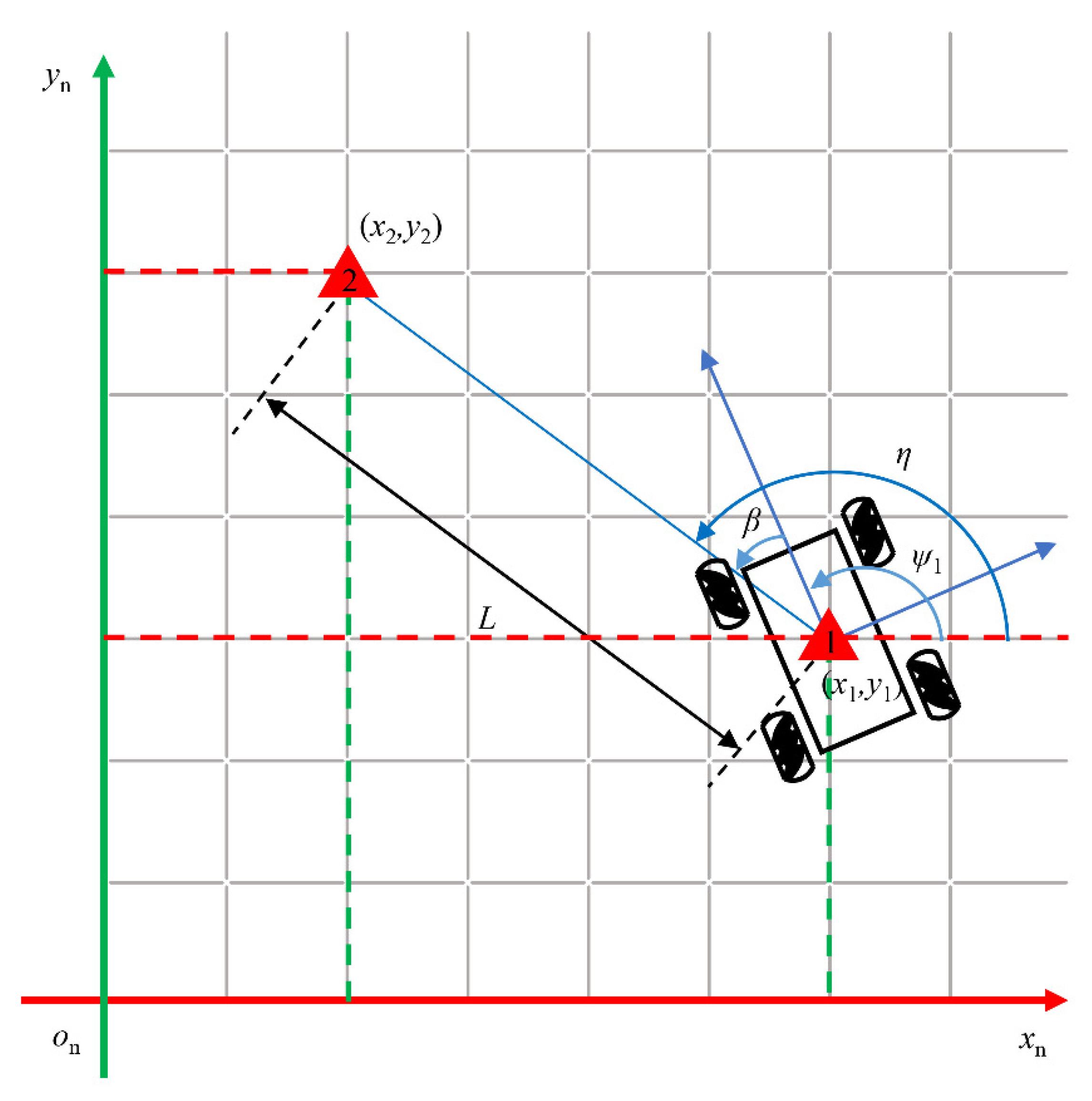
As shown in Figure 13, the robot is at point 1 and needs to reach the point 2 to be lofted. At this time, the position and attitude of the robot at point 1 is $(x_1,y_1,{\psi }_1)$, the position of point 2 is $(x_2,y_2)$ which is provided by the first party. To complete the lofting of point 2, the robot needs to rotate the angle $\beta$ around the geometric center and move forward $L$. The calculations about $\beta$ and $L$ can be solved by known data.

The solving formula are as follows:

$$\{\begin{array}{l}\beta =\eta -{\psi }_1=\arctan 2(\frac{y_2-y_1}{x_2-x_1})-{\psi }_1\hfill \\ L=\sqrt{{(x_2-x_1)}^2+{(y_2-y_1)}^2}\hfill \end{array}$$

(27)

where, $(x_1,y_1)$ is the position of the robot at point 1, ${\psi }_1$ is the attitude of the robot at point 1, $(x_2,y_2)$ is the position of point 2, $\eta$ is the angle between the line of point 1 and point 2 and the positive direction of the x-axis, $\beta$ is the required rotation angle of the robot, $L$ is the distance between point 1 and point 2.

However, it is almost impossible for the robot to accurately rotate the angle $\beta$ or move forward $L$. When the robot deviates from the expected trajectory, it will correct in real-time according to its position and attitude $(x_{now},y_{now},{\psi }_{now})$ at this time. The methods of solving ${\beta }_{now}$ and $L_{now}$ are similar to (27), namely:

$$\{\begin{array}{l}{\beta }_{now}={\eta }_{now}-{\psi }_{now}=\arctan 2(\frac{y_2-y_{now}}{x_2-x_{now}})-{\psi }_{now}\hfill \\ L_{now}=\sqrt{{(x_2-x_{now})}^2+{(y_2-y_{now})}^2}\hfill \end{array}$$

(28)

where, $(x_{now},y_{now})$ is the real-time position of the robot, ${\psi }_{now}$ is the real-time attitude of the robot, ${\eta }_{now}$ is the angle between the line between the real-time position of the robot and point 2 and the positive direction of the x-axis, ${\beta }_{now}$ is the required real-time rotation angle of the robot, $L$ is the distance between the real-time position of the robot and point 2.

7. Experiment and Results

This part mainly introduces the power distribution of the robot and verifies the feasibility of the system, the localization accuracy of the robot is also verified through practical experiments.

7.1. Introduction of Power Distribution

The robot platform introduced in this paper was mainly equipped with wheel encoder, MEMS-IMU, and magnetometer sensors. It is used in combination with a BIM laser lofting instrument, which is an external sensor, to determine the point position in lofting. Among them, the wheel encoder is used to set the velocity of the robot. The BIM laser lofting instrument links with a prism fixed at the top of the robot and outputs the position information of the robot under 20 Hz. After that, the position information is sent to the embedded STM32F103 series processor of the robot through WIFI communication for data processing. MEMS-IMU and magnetometer estimate the robot attitude through EKF. The data is sent to the STM32F103 series processor through serial communication and the fusion algorithm is executed by the processor. The processor has 72 MHz CPU, 125 Dmips, 256 kb flash memory and can output the attitude estimation at 200 Hz.

7.2. Experimental Results

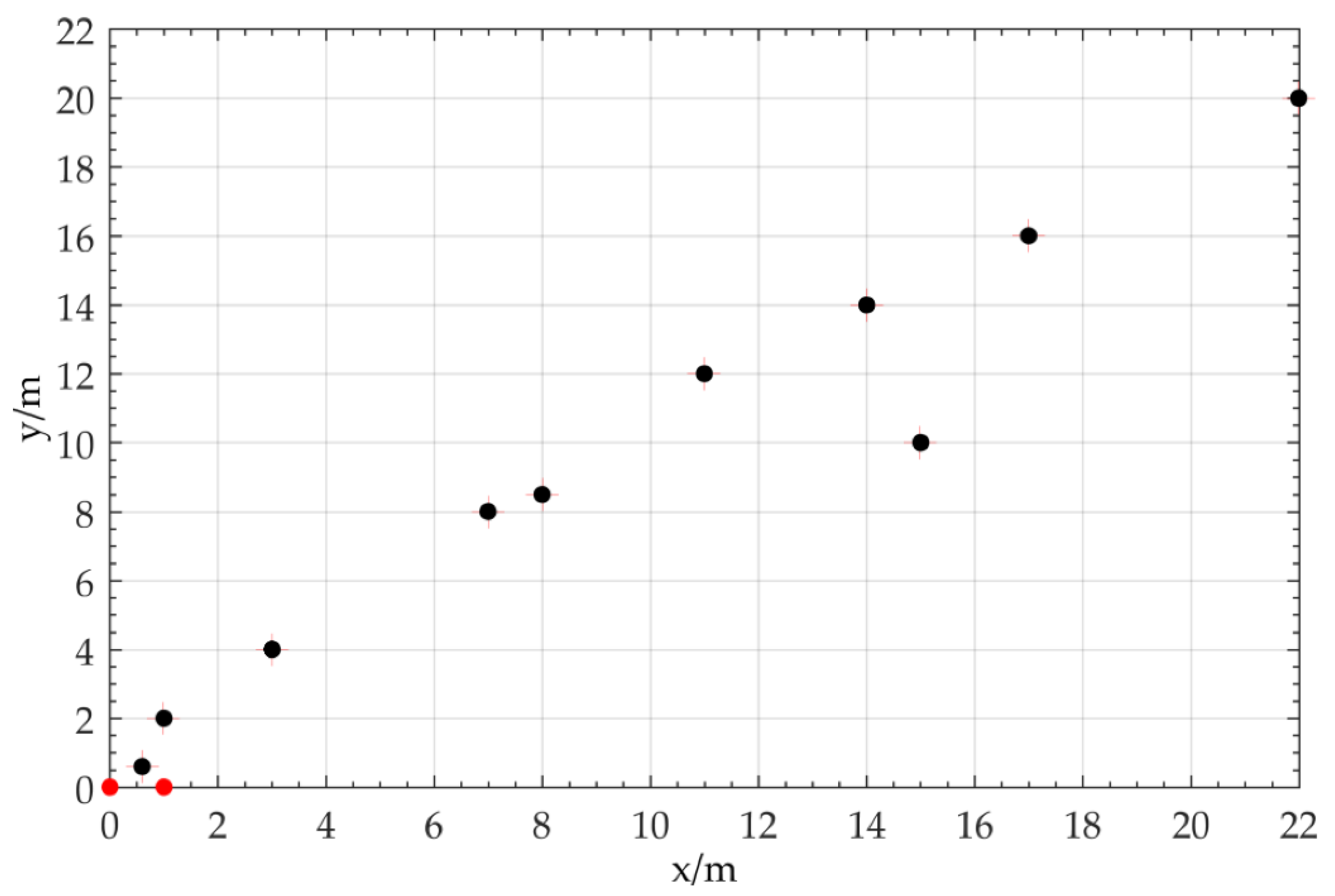
To verify the accuracy of localization, this experiment was carried out in an indoor barrier-free environment. The sensors were pre-corrected and the minor errors in initial orientation and alignment were ignored. We adopted the custom coordinate system method and set the instrument arbitrarily. Figure 14 is the points layout and result diagram of this experiment, 12 points were selected for the experiment, of which 2 red points were the initial points ((0, 0) was the installation position of the BIM laser lofting instrument, and (1, 0) was the initial position of the robot), and the remaining 10 black points were the points to be lofted, ‘+’ were the lofting result of 10 black points. Experimental distance from 0.72 m to 29 m. The experimental results are shown in

Table 3. The results of localization experiment.

Points	Points Position/m	Actual Position/m	Error/mm
Instrument location	(0, 0)
Start point	(1, 0)
1	(0.6, 0.6)	(0.603, 0.593)	7.6
2	(1, 2)	(0.992, 1.993)	10.6
3	(3, 4)	(3.000, 3.991)	9.0
4	(7, 8)	(6.994, 7.993)	9.2
5	(8, 8.5)	(8.004, 8.495)	6.4
6	(15, 10)	(14.993, 10.004)	8.0
7	(11, 12)	(10.994, 11.998)	6.3
8	(14, 14)	(14.005, 13.996)	6.4
9	(17, 16)	(16.995, 16.007)	8.6
10	(22, 20)	(21.994, 19.998)	6.3

.

The localization accuracy of the robot is crucial for lofting. Table 3 shows the positions of ten points to be lofted and the actual localization accuracy. It can be seen from Table 3, the average localization error in the experiment is 7.84 mm, RMSE is 1.427 mm, and the maximum error is the only 10.6 mm, which meets most of the lofting requirements. To compare the lofting time between our method and the traditional method, we use a total station to stake out the same ten points. For 10 points, the robot takes 7.43 min, and the total station takes 19.6 min. It can be seen that the robot lofting method proposed in this paper improves efficiency by about 163.8% compared with the traditional lofting method and reduces manpower.

8. Discussion

The intelligent lofting system proposed in this article has practical application values for many projects, such as indoor decoration and indoor lofting, and can improve the efficiency of lofting under the premise of high enough accuracy.

Table 4. The accuracy control standards for indoor lofting in GB 50210 and GB50242 of China.

	Full Floor Length	Allowable Deviation
Single door window	<30 m	15 mm
	≥30 m	20 mm
Adjacent doors and windows		10 mm
Fire hydrant		20 mm
Plumbing equipment		15 mm
Central position of floral decoration		10 mm

is the accuracy control standards for indoor lofting in GB 50210 and GB50242 of China.

According to Table 3 and Table 4, our method meets the standards of most indoor lofting projects. But for the maximum localization error, we think it is due to the error of the BIM laser lofting instrument itself and robot manufacturing error. The sensors’ resolution and the environment of the experiment site will also have an impact on accuracy. Among them, the lofting environment is one of the main factors that affect accuracy. The rugged ground will have a serious impact on the balance of the Mecanum wheel, which will also affect our subsequent outdoor lofting research. Improving the localization algorithm and the robot motion control theory to further improve lofting accuracy is also one of the future research directions of this paper.

As for the issue of lofting time, whether it is the method proposed in this article or the traditional method, we record the ground marking time as 10s. This time is more realistic, although the marking time of the robot may be shorter in the future. The leveling time of the instrument cannot be ignored, because fast leveling is also one of the advantages of the BIM laser lofting instrument.

9. Conclusions

We propose an intelligent lofting system for the indoor barrier-free plane environment combined with a BIM laser lofting instrument. This method has certain application value for indoor decoration, indoor point layout, indoor equipment pre-placement, etc. In this paper, the design of the robot platform, velocity control, robot localization, and motion control theory are described. From the final experimental results, it can be seen that the method has achieved the expected goal. For the most important localization problem, we propose a method of combining internal and external multi-sensor data to estimate the state of the robot. Compared with the traditional method, the accuracy of this method meets the requirements of most indoor lofting, and the efficiency is higher, and the robot platform runs well.

The proposal of this method has certain significance for some large-area, boring and repetitive indoor lofting work, such as tile position lofting in large office buildings, indoor decoration, factory equipment pre-placement, etc. Compared with the traditional total station lofting method, our method further reduces the manpower through the robot, improves the lofting speed, and expands the sales path of the BIM laser lofting instrument under the premise of ensuring the lofting accuracy. However, its main limitation at present is that it is only suitable for two-dimensional and indoor Barrier-free lofting environment, which is difficult to meet most of the outdoor lofting projects or indoor obstacle environment. The maintenance of the robot also costs.

Further work will adopt more sensors to the system, focus on intelligent lofting in indoor and outdoor obstacle environment, and improve localization algorithm and motion control theory to improve the localization accuracy. We believe that this method can effectively solve the existing problems in lofting and greatly improve lofting efficiency.

References

- Gu, X.; Bao, F.; Cheng, X. Construction Engineering Survey. In Elementary Surveying, 4th ed.; Yang, N., Ed.; Tongji University Press: Shanghai, China, 2011; p. 288. [Google Scholar]
- Paul, S. Using a Transit and Tape. In Construction Surveying & Layout, 1st ed.; William, D.M., Ed.; Building News: Anaheim, UK; Washington, DC, USA, 2002; pp. 43–61. [Google Scholar]
- Luo, Y.; Chen, J.; Xi, W.; Zhao, P.; Qiao, X.; Deng, X.; Liu, Q. Analysis of tunnel displacement accuracy with total station. Measurement 2016, 83, 29–37. [Google Scholar] [CrossRef]
- Qingjuana, S.; Hui, C. Surveying and Plotting Method for the River Channel Section Based on the Total Station and CASS. Procedia Eng. 2012, 28, 424–428. [Google Scholar] [CrossRef] [Green Version]
- Bechar, A.; Vigneault, C. Agricultural robots for field operations: Concepts and components. Biosyst. Eng. 2016, 149, 94–111. [Google Scholar] [CrossRef]
- Hansen, K.D.; Garcia-Ruiz, F.; Kazmi, W.; Bisgaard, M.; la Cour-Harbo, A.; Rasmussen, J.; Andersen, H.J. An Autonomous Robotic System for Mapping Weeds in Fields. In Proceedings of the IFAC Proceedings Volumes, Gold Coast, Australia, 26–28 June 2013; pp. 217–224. [Google Scholar]
- Unal, I.; Kabas, O.; Sozer, S. Real-Time Electrical Resistivity Measurement and Mapping Platform of the Soils with an Autonomous Robot for Precision Farming Applications. Sensors 2020, 20, 251. [Google Scholar] [CrossRef] [Green Version]
- Vithanage, R.K.W.; Harrison, C.S.; De Silva, A.K.M. Autonomous rolling-stock coupler inspection using industrial robots. Robot. Comput. Integr. Manuf. 2019, 59, 82–91. [Google Scholar] [CrossRef] [Green Version]
- Guo, S.; Diao, Q.; Xi, F. Vision Based Navigation for Omni-directional Mobile Industrial Robot. Procedia Comput. Sci. 2017, 105, 20–26. [Google Scholar] [CrossRef]
- Neumann, P.P.; Hüllmann, D.; Bartholmai, M. Concept of a gas-sensitive nano aerial robot swarm for indoor air quality monitoring. Mater. Today Proc. 2019, 12, 470–473. [Google Scholar] [CrossRef]
- AlHaza, T.; Alsadoon, A.; Alhusinan, Z.; Jarwali, M.; Alsaif, K. New Concept for Indoor Fire Fighting Robot. Procedia-Soc. Behav. Sci. 2015, 195, 2343–2352. [Google Scholar] [CrossRef] [Green Version]
- Xu, J.; Zhang, L.; Zhu, Y.; Gou, H. The Application of GPS-RTK in Engineering Measurement and Position. In Proceedings of the 2009 Second International Symposium on Knowledge Acquisition and Modeling, Wuhan, China, 30 November–1 December 2009; pp. 186–189. [Google Scholar]
- Mueller, A.; Himmelsbach, M.; Luettel, T.; Hundelshausen, F.V.; Wuensche, H.-J. GIS-based topological robot localization through LIDAR crossroad detection. In Proceedings of the 2011 14th International IEEE Conference on Intelligent Transportation Systems (ITSC), Washington, DC, USA, 5–7 October 2011; pp. 2001–2008. [Google Scholar]
- Patruno, C.; Colella, R.; Nitti, M.; Reno, V.; Mosca, N.; Stella, E. A Vision-Based Odometer for Localization of Omnidirectional Indoor Robots. Sensors 2020, 20, 875. [Google Scholar] [CrossRef] [Green Version]
- Frías, E.; Díaz-Vilariño, L.; Balado, J.; Lorenzo, H. From BIM to Scan Planning and Optimization for Construction Control. Remote Sens. 2019, 11, 1963. [Google Scholar] [CrossRef] [Green Version]
- Jiang, S.Y. Discussion on the Application of GPS Technology in Bridge Construction Plane Control Net and in Survey of Bridge Axis Lofting. Appl. Mech. Mater. 2014, 580–583, 2842–2847. [Google Scholar] [CrossRef]
- Lee, S.; Lee, S.; Baek, S. Vision-Based Kidnap Recovery with SLAM for Home Cleaning Robots. J. Intell. Robot. Syst. 2011, 67, 7–24. [Google Scholar] [CrossRef]
- Breuer, T.; Giorgana Macedo, G.R.; Hartanto, R.; Hochgeschwender, N.; Holz, D.; Hegger, F.; Jin, Z.; Müller, C.; Paulus, J.; Reckhaus, M.; et al. Johnny: An Autonomous Service Robot for Domestic Environment. J. Intell. Robot. Syst. 2011, 66, 245–272. [Google Scholar] [CrossRef]
- Liu, F.; Li, X.; Wang, J.; Zhang, J. An Adaptive UWB/MEMS-IMU Complementary Kalman Filter for Indoor Location in NLOS Environment. Remote Sens. 2019, 11, 2628. [Google Scholar] [CrossRef] [Green Version]
- Benini, A.; Mancini, A.; Longhi, S. An IMU/UWB/Vision-based Extended Kalman Filter for Mini-UAV Localization in Indoor Environment using 802.15.4a Wireless Sensor Network. J. Intell. Robot. Syst. 2012, 70, 461–476. [Google Scholar] [CrossRef]
- Gregory, D.; Michael, J. Inertial sensors, GPS, and odometry. In Springer Handbook of Robotics, 2nd ed.; Springer: Berlin/Heidelberg, Germany, 2008; Volume 20, pp. 477–479. [Google Scholar]
- Kumar, G.A.; Patil, A.K.; Patil, R.; Park, S.S.; Chai, Y.H. A LiDAR and IMU Integrated Indoor Navigation System for UAVs and Its Application in Real-Time Pipeline Classification. Sensors 2017, 17, 1268. [Google Scholar] [CrossRef] [Green Version]
- Zhang, X.; Shi, H.; Pan, J.; Zhang, C. Integrated navigation method based on inertial navigation system and Lidar. Opt. Eng. 2016, 55, 044102. [Google Scholar] [CrossRef]
- Liu, S.; Atia, M.M.; Karamat, T.B.; Noureldin, A. A LiDAR-Aided Indoor Navigation System for UGVs. J. Navig. 2014, 68, 253–273. [Google Scholar] [CrossRef] [Green Version]
- Suhr, J.K.; Jang, J.; Min, D.; Jung, H.G. Sensor Fusion-Based Low-Cost Vehicle Localization System for Complex Urban Environment. IEEE Trans. Intell. Transp. Syst. 2017, 18, 1078–1086. [Google Scholar] [CrossRef]
- Faralli, A.; Giovannini, N.; Nardi, S.; Pallottino, L. Indoor real-time localisation for multiple autonomous vehicles fusing vision, odometry and IMU data. In Proceedings of the Third International Workshop on Modelling and Simulation for Autonomous Systems, Rome, Italy, 15–16 June 2016; pp. 288–297. [Google Scholar]
- Jiang, X.; Chen, G.; Capi, G.; Ishll, C.; Mai, Y.; Lai, Y. Development of an indoor positioning and navigation system using monocular SLAM and IMU. In Proceedings of the First International Workshop on Pattern Recognition, Tokyo, Japan, 11 July 2016; p. 100111L. [Google Scholar]
- Chen, M.; Yang, S.; Yi, X.; Wu, D. Real-time 3D mapping using a 2D laser scanner and IMU-aided visual SLAM. In Proceedings of the 2017 IEEE International Conference on Real-time Computing and Robotics (RCAR), Okinawa, Japan, 14–18 July 2017; pp. 297–302. [Google Scholar]
- Deilamsalehy, H.; Timothy, C. Sensor fused three-dimensional localization using IMU, camera and LiDAR. In Proceedings of the 2016 IEEE SENSORS, Orlando, FL, USA, 30 October–2 November 2016; pp. 376–378. [Google Scholar]
- Nieuwenhuisen, M.; Droeschel, D.; Beul, M.; Behnke, S. Autonomous Navigation for Micro Aerial V ehicles in Complex GNSS-denied Environment. J. Intell. Robot. Syst. 2016, 84, 199–216. [Google Scholar] [CrossRef]
- Aghili, F.; Salerno, A. Driftless 3D Attitude Determination and Positioning of Mobile Robots By Integration of IMU With Two RTK GPSs. IEEE/ASME Trans. Mechatron. 2013, 18, 21–31. [Google Scholar] [CrossRef]
- Liu, F.; Chen, Y.; Li, Y. Research on Indoor Robot SLAM of RBPF Improved with Geometrical Characteristic Localization. In Proceedings of the IEEE 2017 29th Chinese Control And Decision Conference (CCDC), Chongqing, China, 28–30 May 2017; pp. 3325–3330. [Google Scholar]
- Lee, T.J.; Kim, C.H.; Cho, D. A Monocular Vision Sensor-Based Efficient SLAM Method for Indoor Service Robots. IEEE Trans. Ind. Electron. 2019, 66, 318–328. [Google Scholar] [CrossRef]
- Du, H.; Wang, W.; Xu, C.; Xiao, R.; Sun, C. Real-Time Onboard 3D State Estimation of an Unmanned Aerial Vehicle in Multi-Environment Using Multi-Sensor Data Fusion. Sensor 2020, 20, 919. [Google Scholar] [CrossRef] [PubMed] [Green Version]
- Yi, J.; Wang, H.; Zhang, J.; Song, D.; Jayasuriya, S.; Liu, J. Kinematic Modeling and Analysis of Skid-Steered Mobile Robots With Applications to Low-Cost Inertial-Measurement-Unit-Based Motion Estimation. IEEE Trans. Robot. 2009, 25, 1087–1097. [Google Scholar]
- Ferreira, J.C.; Resende, R.; Martinho, S. Beacons and BIM Models for Indoor Guidance and Location. Sensors 2018, 18, 4374. [Google Scholar] [CrossRef] [PubMed] [Green Version]
- Gfrerrer, A. Geometry and kinematics of the Mecanum wheel. Comput. Aided Geom. Des. 2008, 25, 784–791. [Google Scholar] [CrossRef]
Figure 1.
The framework of data integration.
Figure 2.
General design scheme of intelligent lofting system.
Figure 3.
Overall design of robot platform.
Figure 4.
Mecanum wheel: (a) The structure of Mecanum; (b) The force model of bottom wheel.
Figure 5.
The force model of robot: (a) Force model of clockwise rotation; (b) Simplified force model.
Figure 6.
Kinematic model of the robot.
Figure 7.
Building Information Modeling (BIM) laser lofting instrument: (a) The introduction of Topcon LN-100; (b) Sokkia 360° prism matched with Topcon LN-100.
Figure 8.
BIM: (a) A teaching building of Tongji University; (b) The first floor of the building.
Figure 9.
The methods of instrument layout: (a) Resection; (b) Reference Axis (Base Point and Reference Axis) Measurement; (c) Backsight Point (Known Point) Measurement; (d) Backsight Point (Reference Axis on the Base Point) Measurement.
Figure 10.
The relationship between acceleration and attitude.
Figure 11.
Pitch angular velocity and time function graph of gyroscope.
Figure 12.
The diagram of attitude solution.
Figure 13.
Motion Control of the robot.
Figure 14.
Points layout and result diagram of the experiment.