Article

Estimation of Nitrogen in Rice Crops from UAV-Captured Images

by
Julian D. Colorado
1,*,
Natalia Cera-Bornacelli
1,
Juan S. Caldas
1,
Eliel Petro
2,
Maria C. Rebolledo
2,3,
David Cuellar
1,
Francisco Calderon
1,
Ivan F. Mondragon
1 and
Andres Jaramillo-Botero
4,5
1
School of Engineering, Pontificia Universidad Javeriana Bogotá, Carrera 7 No. 40-62, Bogotá 110231, Colombia
2
International Center for Tropical Agriculture (CIAT), Km 17 Recta Cali-Palmira, Cali 110231, Colombia
3
CIRAD, UMR AGAP, F-34398|Univ Montpellier, CIRAD, INRA, Montpellier SupAgro, 34000 Montpellier, France
4
Chemistry and Chemical Engineering Division, California Institute of Technology, Pasadena, CA 91125, USA
5
Electronics and Computer Science, Pontificia Universidad Javeriana Cali, Calle 18 No. 118-250, Cali 760031, Colombia
*
Author to whom correspondence should be addressed.
Remote Sens. 2020, 12(20), 3396; https://0-doi-org.brum.beds.ac.uk/10.3390/rs12203396
Submission received: 2 July 2020 / Revised: 17 September 2020 / Accepted: 22 September 2020 / Published: 16 October 2020
(This article belongs to the Special Issue UAVs for Vegetation Monitoring)

Abstract

:
Leaf nitrogen (N) directly correlates to chlorophyll production, affecting crop growth and yield. Farmers use soil plant analysis development (SPAD) devices to calculate the amount of chlorophyll present in plants. However, monitoring large-scale crops using SPAD is prohibitively time-consuming and demanding. This paper presents an unmanned aerial vehicle (UAV) solution for estimating leaf N content in rice crops, from multispectral imagery. Our contribution is twofold: (i) a novel trajectory control strategy to reduce the angular wind-induced perturbations that affect image sampling accuracy during UAV flight, and (ii) machine learning models to estimate the canopy N via vegetation indices (VIs) obtained from the aerial imagery. This approach integrates an image processing algorithm using the GrabCut segmentation method with a guided filtering refinement process, to calculate the VIs according to the plots of interest. Three machine learning methods based on multivariable linear regressions (MLR), support vector machines (SVM), and neural networks (NN), were applied and compared through the entire phonological cycle of the crop: vegetative (V), reproductive (R), and ripening (Ri). Correlations were obtained by comparing our methods against an assembled ground-truth of SPAD measurements. The higher N correlations were achieved with NN: 0.98 (V), 0.94 (R), and 0.89 (Ri). We claim that the proposed UAV stabilization control algorithm significantly improves on the N-to-SPAD correlations by minimizing wind perturbations in real-time and reducing the need for offline image corrections.

Graphical Abstract

1. Introduction

Farmers use soil plant analysis development (SPAD) devices as a field diagnostic tool to estimate nitrogen (N) content in the plant and to predict grain yield [1,2]. For rice crops, N provides critical insight into plant-growth, crop yield, and biomass accumulation [3]. Furthermore, monitoring N allows farmers to properly adapt crop management practices [4,5]. However, using SPAD devices for crop diagnosis is still time consuming. With the advent of low-cost unmanned aerial vehicles (UAVs), several authors have reported faster and accurate remote sensing tools and methods [6,7] to estimate the N canopy from aerial multispectral imagery [8,9]. One of the most common methods used, relies on sensing the canopy reflectance in both visible (VIS) and near-infrared (NIR) wavelengths, using hyperspectral sensors [10,11,12,13].
Multiple vegetation indices (VI) have been established to associate specific spectral reflectance wavelengths with the crop variables of interest [14,15]. Although these VIs can be used to estimate the N contents in rice plants, there is no single standard set of VIs that works across all crop stages, rice varieties, soils, and atmospheric conditions. Most of the existing body of work associated with the estimation of N contents in plants, has been conducted using multi-variable regressions [5,16], in which linear functions are defined by combining and weighting each VI according to the regression model. This approach is simple, but sometimes inaccurate since the evolution of the crop tends to exhibit highly nonlinear effects that affect the N content over time. Machine and deep learning methods have recently gained traction, in solving these issues. Machine learning has the potential to drive significant breakthroughs in plant phenotyping [17,18,19,20].
For canopy N estimation, training machine learning algorithms requires the precise extraction of VI features from the aerial multispectral imagery. Several authors have applied data fusion methods from different sensors [21,22,23] for applying image mosaicing techniques [24,25,26,27], computing crop surface models based on dense image matching (DIM) techniques [28], or applying photogrammetry methods that are computationally expensive [26,27,29,30]. Other approaches rely on the real-time segmentation and image registration for the extraction of relevant features associated with the leaf/canopy N, including edge detection thresholding, color histograms, and clustering (otsu, K-means, watershed) [31,32,33].
In this work, we improve on the stabilization control of the UAV for acquiring accurate plot imagery, instead of relying on mosaicing or photogrammetry methods. Commercial UAV quadrotors used for the monitoring of the canopy N usually come with a proportional-integral-derivative (PID) waypoint navigation autopilot. The lack of proper UAV angular stabilization in the presence of large wind perturbations limits the accuracy of image registration algorithms, therefore affecting the estimation of canopy N content through image processing. To address this problem, we demonstrate a nonlinear trajectory-tracking controller that enables precise UAV positioning through a stabilization/attitude control loop. We call this method backstepping+ desired angular acceleration function (BS + DAF). This approach incorporates UAV aerodynamics information within the control law to produce roll and pitch acceleration commands to reduce abrupt angular acceleration changes caused by external wind disturbances. This added compliance enables the UAV to hover over the crop plots precisely, which in turn allows for capturing imagery that can be individually processed in real-time.
Here, we combine an autonomous UAV to acquire multispectral imagery from a crop, with machine learning methods as a means to high-throughput nitrogen content estimation. Three major contributions are involved:
(i)
The development and validation of a novel UAV attitude control called BS+DAF. The UAV captures multispectral imagery with relevant above-ground data that must correlate with the SPAD measurements at the ground-level of the crop. The proposed controller is aimed at maintaining precise angular stabilization during flight by properly rejecting wind disturbances, enabling improvements in the estimations of N.
(ii)
The application and validation of a segmentation algorithm called GrabCut [34], instead of the traditional edge detection thresholding methods, color histograms, and clustering techniques used in agriculture. The GrabCut approach achieves smooth pixel information with richer detail of the canopy structure, enabling the accurate segmentation of the multispectral imagery and the proper VI-based feature extraction.
(iii)
The integration of machine learning methods to process nonlinear N dynamics with the calculations of the VIs during all stages of crop growth. A comprehensive characterization of the crop by designing a ground-truth dataset with several contrasting rice genotypes and accurate direct measurements of leaf nitrogen (training model).

2. Materials and Methods

2.1. System

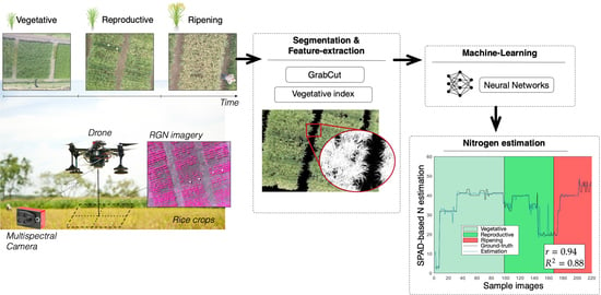
Figure 1 details the proposed approach. Our UAV is a quadrotor called the AscTec Pelican (manufactured by Intel’s Ascending Technologies (https://robots.ros.org/astec-pelican-and-hummingbird/)). This UAV comes with a C++ software development kit (SDK) that enables onboard code development with ease. A high-level Atom Intel processor (HLP) offers enough computing power to run solutions in real-time, whereas a low-level processor (LLP) handles the sensor data fusion and rotor control with an update rate of 1kHz. As shown in Figure 1, we developed a closed-loop attitude controller to drive the low-level rotor’s control running in the LLP. This control method depends on the dynamics of the UAV to properly reject wind disturbances and keep the UAV steady. During flight, a dataset of multispectral imagery is precisely collected aiming at the above-ground estimation of nitrogen by using machine learning methods. In previous work [35], our UAV system was tested during two years of in-field experiments with the aim of estimating above ground biomass accumulation. Here, we have extended the capabilities of the system in Figure 1 by developing and integrating novel methods for UAV flight control, multispectral imagery segmentation for VI feature extraction, and their impact on nitrogen estimation using machine learning algorithms.
The UAV was equipped with the Parrot Sequoia multispectral sensor (https://www.parrot.com/business-solutions-us/parrot-professional/parrot-sequoia) fabricated with 4 separate bands: green, red, red-edge, and near-infrared. The camera offers a resolution of 1280 × 960 for each independent spectral sensor, yielding a crop-to-image resolution of 1.33 cm/pixel according to the flying altitude of 20 m. In addition, the multispectral camera comes with a radiometric calibration target that enables offline reflectance calibration across the spectrum of light captured by the camera, and an onboard irradiance sensor designed to correct images for illumination differences, all of which enables its outstanding performance in cloudy conditions, as evaluated in [36]. In our application, this calibration procedure was executed prior to any flight mission of the UAV. Additional sensors such as an IMU, magnetometer, and GPS are also embedded within the sunshine sensor. 
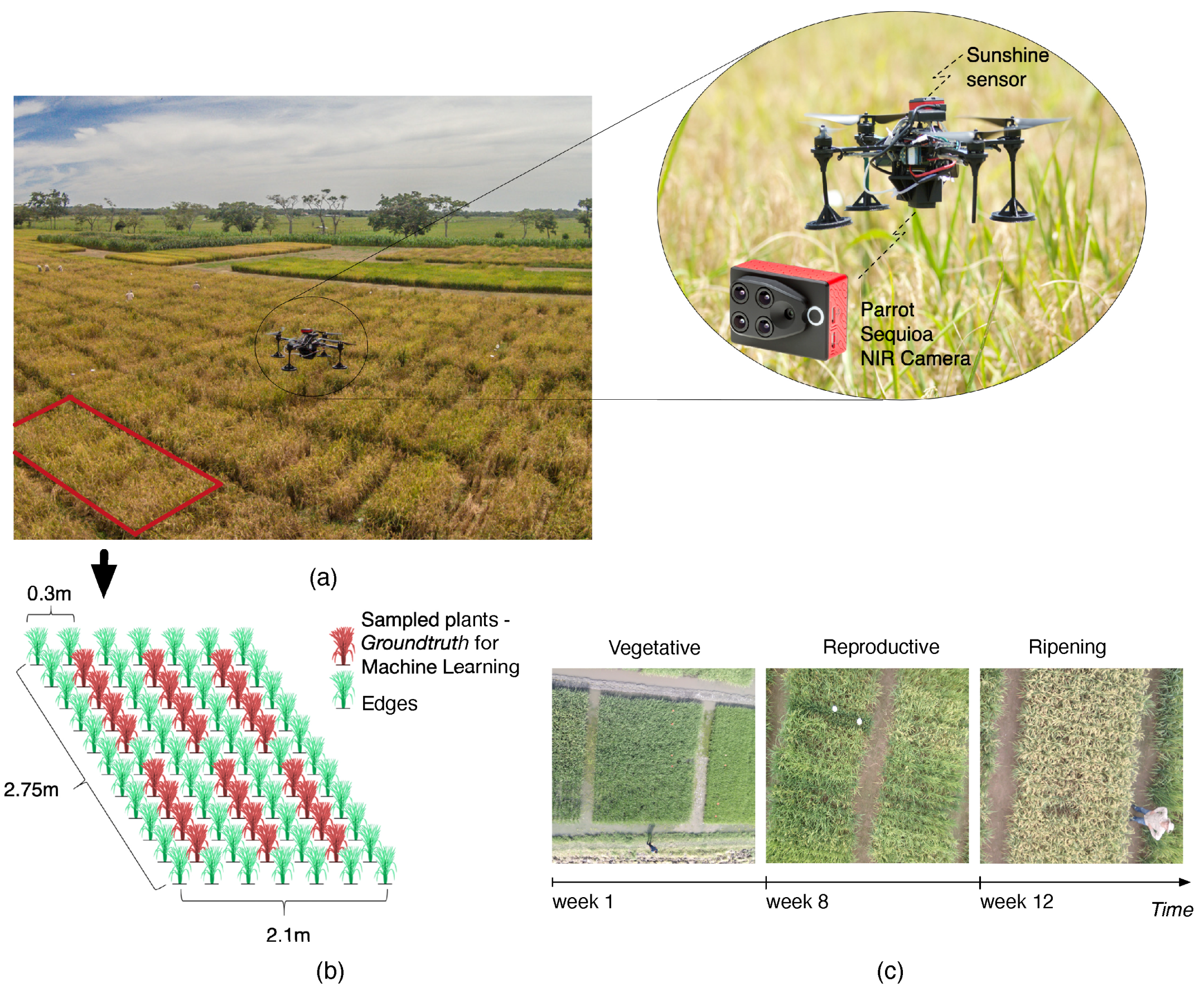
Figure 2a depicts the mounted camera setup, while Table 1 details the general specifications of our system.

2.2. Rice Crops

The crops were designed with 3 spatial repetitions containing 8 contrasting rice genotypes in terms of N concentration, biomass accumulation, and flowering: FED50, MG2, ELWEE, NORUNKAN, IR64, AZUCENA, UPLRI7, and LINE 23. These rice varieties have a phenological cycle ranging between 86–101 days , as detailed in Figure 3b. The experimental design consisted of six months of in-field sampling with three different planting crops. For each experiment, the amount of applied nitrogen and water was modified as follows:
  • Experiment 1: 200 kgha 1 of nitrogen and limited crop irrigation.
  • Experiment 2: 200 kgha 1 of nitrogen with permanent crop irrigation.
  • Experiment 3: 100 kgha 1 of nitrogen with permanent crop irrigation.
Experimental trials were conducted during the dry season. To assess the effects of limited and permanent irrigation on the crops, leaf temperature (MultispeQ (https://www.photosynq.com)), and soil humidity (AquaPro (http://aquaprosensors.com)) were constantly monitored. Fertilizers were applied accordingly in order to maintain the crops through the phenological cycle. Given that, the same amount of fertilizers were applied for the experiments: 60 kgha 1 of P 2 O 5 (diammonium phosphate) and 130 kgha 1 of K 2 O (potassium chloride), as detailed in the experimental protocol available in the Supplementary Materials section.
Figure 2 details some characteristics of the crop. As shown in plots (a), (b), the length of a plot was about 2.75 m with a distance between plants of 25 cm and 30 cm between rows. Within each plot, we defined 6 sampled areas with 1 linear meter in length (containing four plants). A ground-truth was defined based on the direct measurements of plant chlorophyll using a SPAD 502 Plus meter (Konica-Minolta) over these sampled areas. Measurements from the crop were obtained during three stages of rice growth: vegetative, reproductive, and ripening. Figure 3b details the specifications of the crop experiments reported here.
Table 2 details how the dataset was collected, in which the SPAD value corresponds to the average of 24 measurements conducted over each plot, as depicted in Figure 3b. All ground-truth data are available through the Open Science Framework in the Supplementary Materials section. On the other hand, Figure 3a shows the linear correlation used to relate the measured SPAD value with the leaf-blade N concentration [37].
As mentioned, vegetation indices are widely used to quantify both plant and soil variables by associating certain spectral reflectances that are highly related to variations in canopy chemical components such as nitrogen. From the extensive list of vegetation indices (VIs) available [38,39,40,41], we selected 7 VIs with sufficient experimental evidence and quantitative trait loci (QTL)-based characterization regarding their high correlation with rice nitrogen [42]. Table 3 details the selected VIs. These formulas are applied in different wavelengths for taking into account the changes in canopy color, since several factors affect the spectral reflectances of the crop: solar radiation, plant morphology and color, leaf angles, undergrowth, soil characteristics, and water.
In our system, the parrot sequoia camera has a solar radiation sensor that compensates the light variations in the canopy. The change in the rice canopy color is perhaps the most notable variation during the phenological cycle. In the vegetative stage, the green color is predominant whereas in the reproductive stage, panicle formation starts and thus yellow features appear in the images. In ripening, the maturation of the plants occur while the leaves begin to senesce, turning the yellow color predominant. These changes can be observed in Figure 2c. Furthermore, different wavelengths of light have a different level of plant absorption depending on the leaf composition given by several genetic traits. In particular, the relation between the selected VIs in Table 3 with the photosynthetic activity and canopy structural properties has allowed the association of certain spectral reflectances that are highly related to the physico-chemical canopy N variations in plants, especially the green, red, red-edge, and near infrared bands.
The selected VIs exhibit a strong dependence on the NIR reflectance due to leaf chlorophyll absorption, providing an accurate approach to determine the health status of the plants and the canopy N. Most of the existing body of research focused on multispectral-based N estimations [14,21,40,42,43], combine the information provided by several vegetation indices in order to avoid saturation issues. For instance, the NDVI, which is one of the most common VIs used, tends to saturate with dense vegetation. In turn, the NDVI alone is not accurate during the reproductive and ripening stages of rice growth. Here, we combine several VIs across the crop stages, to ensure data on wavelengths located in the red-edge and another spectral reflectances that accurately express the healthy status of the leaves (higher NIR and green-band readings).

2.3. UAV Stabilization Control

The estimation of the canopy N requires the precise extraction of Vegetative Index features from the acquired multispectral imagery. Capturing aerial images during UAV hovering that accurately matches with the GPS positions of the SPAD measurements at ground-level is essential.
As previously detailed in Figure 1, three closed-loop controllers are needed to regulate: (i) the X-Y position based on GPS feedback, (ii) the Z altitude based on barometric pressure and laser readings (pointing downwards), and (iii) the ϕ , θ , ψ attitude based on IMU data. The UAV is constantly subjected to wind disturbances that cause unsteady angular motions and therefore imprecise trajectory tracking. Consequently, aerial imagery captured across the crop with the UAV system is affected. To overcome this issue, we replaced both roll and pitch PID-based controllers by a robust nonlinear backstepping (BS) control.
The classical BS method has several advantages. It explicitly takes into account the nonlinearities of the UAV model defined in Equation (A2) (see Appendix A), and most importantly, allows the incorporation of a virtual control law to regulate angular accelerations. For this, we have derived a desired acceleration function (DAF) for roll and pitch. This enhanced controller is called backstepping+DAF (BS+DAF). Our goal is to use the dynamics equations of motion (EoM) defined in Algorithm A1 within the control law in order to compensate for abrupt angular acceleration changes, concretely in roll and pitch. The DAF terms improve the responsiveness of the control law to external perturbative forces. Appendix B details the control law derivation for roll and pitch.
The BS + DAF control supports on the Lyapunov stability concept that guarantee asymptotic stabilization around the equilibrium points. For our application, we require both roll ϕ a pitch θ angles to remain in zero while the UAV is hovering above the crop for capturing multispectral imagery, i.e.,  e ϕ = ϕ d ϕ 0 and e θ = θ d θ 0 . Otherwise, the set-point references for both roll and pitch controllers are defined by the X-Y position controller.
As previously mentioned, high wind-speed perturbations affect the UAV during hovering. Nonetheless, our controller law is sensitive to angular acceleration changes caused by external wind disturbances, thanks to both error dynamics ( e 2 ) and the DAF terms ( ϕ ¨ d ) in Equation (A18) (Appendix B). Given that, we present how to model the effects of the wind over the UAV aerodynamics, by following the wind effect model (WEM) developed by [44]. 
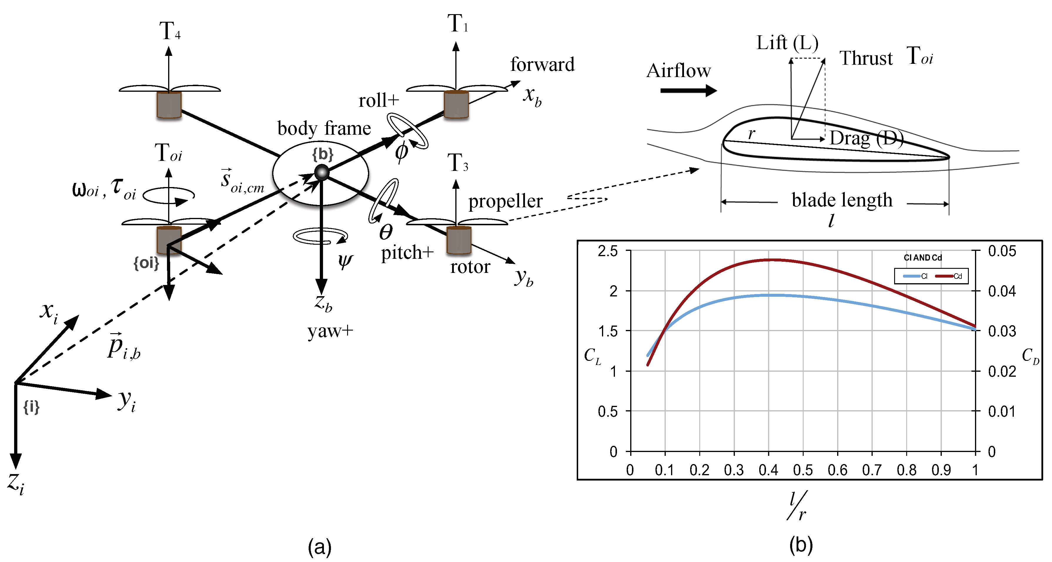
Figure 4 details the control architecture and how the WEM module has been incorporated as an external disturbance acting on the UAV body frame.
The WEM defines the relationship between the oblique airflow acting on a propeller and the resulting forces and moments applied onto the UAV. In our quadrotor system, the oblique airflow form and angle of 90o with the propeller azimuth angle. In terms of aerodynamics, the incoming airflow induces an increase in vertical thrust ( T o i ), a side force (F w i n d ), and a pitching moment (M w i n d ). The WEM presented by [44] uses blade element momentum theory to determine the aforementioned effects. Here, we are interested in incorporating the effects caused to the thrust and the pitching moment (M w i n d ) as a function of the magnitude of a given wind speed vector V w i n d and the rotational speed ω of each propeller driven by the rotor’s model. In this regard, the WEM is defined as:
M w i n d = c o s β + π 2 s i n β + π 2 0 s i n β + π 2 c o s β + π 2 0 0 0 1 M p r o p 0 0 + l 2 C 4 T 4 C 2 T 2 C 1 T 1 C 3 T 3 0
The angle β determines the direction of the V w i n d vector. Depending on the direction of the applied relative wind, certain propellers will be more affected by this external disturbance. Tran et al., in [44,45], propose the use of a weight function that assigns values between 0 to 1, where the maximum value of 1 means the propeller is directly exposed to the wind. In Equation (1), C corresponds to the weighting vector that affects the thrust T generated by each propeller. The parameter l is the distance between non-adjacent propellers and M p r o p is:
M p r o p = C 1 C 2 C 3 C 4 τ 1 τ 2 τ 3 τ 4
Therefore, the scale of the weighting vector C is defined based on the magnitude of the applied wind speed vector and the corresponding direction (the β angle between the relative wind vector pointing towards the UAV body frame). In addition, the rotor’s speeds ω are required to calculate the augmented thrusts T and torques τ (weighted by C). Further details on this model can be found in [44,45].
Section 3.1 and Section 3.3 present the results regarding the impact of precise UAV positioning on the accurate estimation of the canopy N through the entire phenological cycle.

2.4. Multispectral Image Segmentation

Multispectral imagery is evaluated by using a multispectral image segmentation method called GrabCut [34]. The original method is widely used for its ease of implementation and for the excellent results in generating a binary classification; however, it suffers from the drawback of being a semi-manual algorithm. The original GrabCut method requires a manual input during the algorithm iteration in order to properly determine both background and foreground pixel values.
This section introduces a modified version of the GrabCut algorithm that is fully automatic, thanks to an added refinement step using a guided filtering [46] to extract the relevant pixel information associated with the plant’s canopy. Our approach solves an optimization problem using an energy function that allows the proper labeling of texture in the multispectral image by using a Gaussian mixture model. As mentioned, we use a refinement process based on a guided-filter by taking into account information from all band channels of the multispectral camera: green, red, red-edge, and near-infrared. The resultant multispectral image-mask includes only relevant pixel information that accurately represents the canopy for the estimation of N.

2.4.1. GrabCut Segmentation

The GrabCut method requires an initial model known as a trimap. This model consists of a partition of the input image into three regions: a foreground T F , a background T B , and a region with pixels that result from the combination of the foreground and background colors T U .
The image is modeled as an array of values z = ( z 1 , , z N ) , and the output segmentation can be a channel of values between 0 and 1 or a hard segmentation with a binary assignment (0 or 1). The segmentation is written as α ̲ = ( α 1 , α N ) with 0 α n 1 , or  α n = { 1 , 0 } .
The GrabCut algorithm also requires a model for the distribution of the foreground/background colors and gray levels. This distribution can be represented as a histogram directly assembled from T F and T B , as: θ ̲ = { h ( z ; a ) , a = 0 , 1 } . Under this trimap model, the segmentation algorithm determines the values of α from the image z and the distribution model θ ̲ . The  α values are calculated from an energy minimization function, as:
E ( α ̲ , θ ̲ , z ) = U ( α ̲ , θ ̲ , z ) + V ( α ̲ , z ) ,
where the sub-function U evaluates the fitness by assigning a low score if the segmentation ( α ) is consistent with the image z , defined as follows:
U ( α , θ , z ) = n ln h ( z n ; α n )
Instead of using the histogram as the estimator of the probability density function, the algorithm uses a Gaussian mixture model in order to take into account the information coming from all channels.
V ( α ̲ , z ) = γ ( m , n ) C [ α n α m ] e β ( z m z n ) 2
In Equation (5), the sum set C 3 × 3 refers to the neighbors pixels in a given window, and the the term β can be calculated according to Equation (6).
β = 1 2 E ( z m z n ) 2
By using the global minimum in 7, the image segmentation is estimated as:
α ^ ̲ = arg min α ̲ E ( α ̲ , θ ̲ , z )
Algorithm 1 details the original GrabCut method. In order to eliminate the third manual step of the algorithm, a fixed background image T B mask is used during the iteration, and a guided-filter refinement process is applied to achieve an automatic segmentation, as detailed in Algorithm 2.  
Algorithm 1: Original GrabCut algorithm.
  • Step 1: Initialization of T B , T F , T U .
  • Initialize the trimap T F as the foreground
  • Initialize the trimap T B as the background
  • All remaining pixels are set as a possible foreground pixels T U F
  • Step 2: Iterative minimization.
  • Assign and learn GMM
  • Minimize energy function
  • Estimate segmentation image α
  • IF image α have visible errors GO to Step 3
  • Step 3: User editing.
  • Use the segmented image α as the new possible foreground pixels T U F
  • Input pixel hints for T B and T F
  • GO to Step 2
Algorithm 2: Modified GrabCut with guided filter calculation. In the algorithm, E r ( I ) denotes a function that calculates the image mean over a radius r, the operations . * and . / denotes the matrix element-wise calculation, and q is the image output.
  • Step 1: Initialization of T B , T F and T U .
  • Initialize the trimap T F as the foreground
  • Initialize the trimap T B as the background
  • All remaining pixels are set as a possible foreground pixels T U F
  • Step 2: Iterative minimization.
  • Assign and learn GMM
  • Minimize energy function
  • Estimate segmentation image α
  • Step 3:Input image p, input guidance I, radius r, and regularization ϵ .
  • 1: μ I E r ( I ) , μ p E r ( I ) , C o r r I E r ( I . * I ) , C o r r I p E r ( I . * p ) .
  • 2: σ I 2 C o r r I μ I .* μ I , σ I p 2 C o r r I p μ I .* μ p
  • 3: a σ I p 2 ./ ( σ I 2 + ϵ ) , b μ p a . * μ I
  • 4: μ a E r ( a ) , μ b E r ( b )
  • 5: q = μ a .* I + μ b

2.4.2. Guided Filter Refinement

The guided filter (GF) [46] can be defined as a convolutional Bilateral Filter with a faster response due to its O ( N ) computational complexity. In this regard, the output of each pixel denoted as q can be expressed as a weighted average over the convolutional window W ( i , j denote the pixel coordinates):
q i = j W i j p j
The GF implies that an image can be filtered using the radiance of another image as guidance. We exploited this concept to filter our segmented plot mask created with the GrabCut algorithm, with the aim of refining the segmented image with the original image as guidance. In this regard, the weight used by the GF is given by:
W i j G F ( I ) = 1 | ω | 2 k ; ( i , j ) ω k 1 + ( I i μ k ) ( I j μ k ) σ k 2 + ϵ ,
where W i j G F depends entirely of the guidance image I. The parameters μ k and σ k 2 are the mean and variance of the guidance image I estimated over a window w k , ϵ denotes a regularization parameter and | ω | is the number of pixels in the window w k .
Section 3.2 presents the results of applying the proposed modified version of GrabCut, by comparing the method against traditional segmentation techniques such as thresholding, K-means, meanshift, but also against the original semi-manual GrabCut method.

2.5. Machine Learning for N Estimations

As detailed in Table 2, the ground-truth for training machine learning (ML) algorithms was defined based on the direct measurements of plant chlorophyll using a SPAD 502 Plus meter (Konica-Minolta) over these sampled areas, as depicted in Figure 1. Datasets contain the measured SPAD value that directly correlates with the leaf-blade N concentrations by following the linear correlation [37] defined in Figure 3a. In this regard, measurements from the crop were obtained during three stages of rice growth: vegetative, reproductive, and ripening, in which 3 trials were conducted per crop stage. These datasets are the result of 10 flights per trial, capturing around 500 images, and yielding a database of 1500 images per stage. Since 3 trials were conducted per crop stage, around 13 , 500 images were processed in this work. Figure 3b details the experimental specifications.
The ML methods were trained with a set of images accounting for the 60 % of the entire database. For the final estimations of leaf nitrogen, we used the remaining 40 % of the database (testing phase of the ML methods). The entire imagery dataset and the ground-truth available in the 
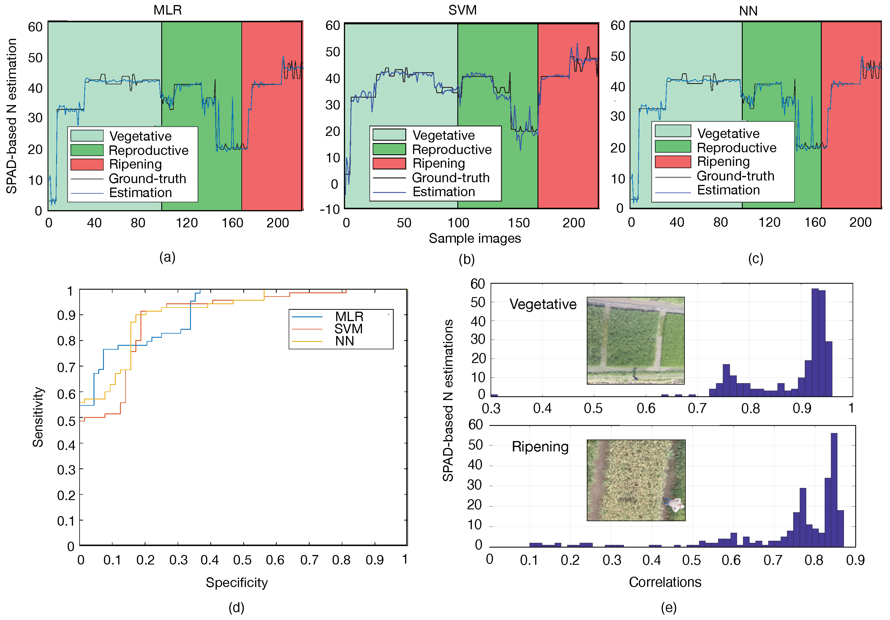
Supplementary Materials section. Here, we report on the use of classical ML methods based on multi-variable linear regressions (MLR), support vector machines (SVM), and artificial neural networks (NN) for the estimation of the canopy N.
For MLR models, the VIs from Table 3 were combined by following the formula: N = β 0 + k = 1 7 β k ( V I ) k , where the parameter β k changes accordingly to the growth stage of the plant, by weighting each VI independently. In this regard, each crop stage will have an independent MLR model that linearly fits the N content.
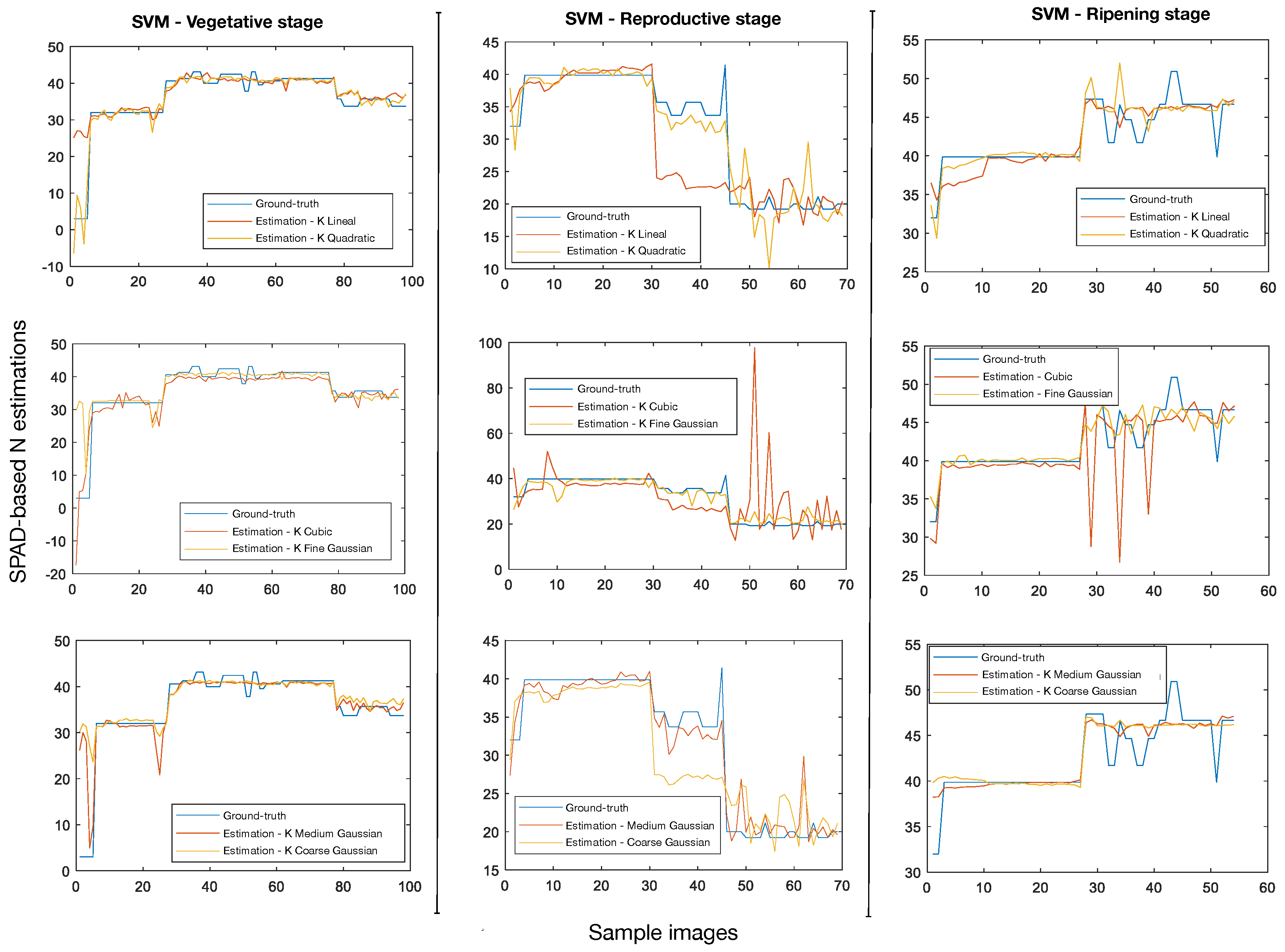
With the aim of improving the adaptability of the estimation models by considering several nonlinear effects (dense vegetation, optical properties of the soil, and changes in canopy color), this section presents the estimation results using support vector machines (SVM) and artificial neural networks (NN). SVM models were used with different kernel functions with the aim of determining the proper mathematical function for mapping the input data. Six different kernels based on linear, quadratic, cubic, and Gaussian models will be tested for each crop stage independently.
Contrarily to the MLR and SVM methods, in which N estimation models are determined for each crop stage independently, neural networks enable the combination of the entire dataset (SPAD values and VI extracted features) into a single model that fits for the entire crop phenological stages. Several non-linear training functions are tested with different hidden layers. In addition, we discarded the use of deep-learning methods such as convolutional neural networks (CNN), due to the high computational costs associated to the pooling through lots of hidden layers in order to detect data features. For this application, we use well-known vegetative index features (reported in Table 3) that have been widely used and validated in the specialized literature [14,40,42]. Other image-based features such as color, structure, and morphology do not work well with multispectral imagery of 1.2 mega-pixel in resolution, compared to the 16 mega-pixel in the RGB image. In fact, the main advantage of using VIs (as features for training), relies on having information at different wavelengths, providing key information of the plant health status related to N.
In Section 3.3, we report a comprehensive comparison among multi-variable linear regressions (MLR), support vector machines (SVM), and artificial neural networks (NN) for the estimation of the canopy N. We used three metrics based on the root mean square error ( R M S E ), Pearson’s linear correlation (r), and coefficient of determination ( R 2 ), detailed as follows:
R M S E = 1 n i = 1 n ( N ^ i N i ) 2 r = i = 1 n ( N i N ¯ ) i = 1 n ( N i N ¯ ) 2 R 2 = i = 1 n ( N i N ^ i ) 2 i = 1 n ( N i N ¯ ) 2
where n is the total number of samples, N is the measured value (SPAD scale cf. Figure 3a), N ^ is the estimated nitrogen, and  N ¯ is the mean of the N values. In this application, the Pearson’s metric indicates the linear relationship between the estimated value of N VS the measured one (ground-truth). On the other hand, the  R 2 metric is useful since it penalizes the variance of the estimated value from the measured one.
As mentioned, the ML models require the calculation of the VI formulas presented in Table 3, in order to determine the input feature vector. Every image captured by the UAV is geo-referenced with the DGPS system with a position accuracy of 35 [cm] (see Table 1). Given that, aerial imagery is registered by matching consecutive frames according to a homography computed with the oriented features from accelerated segment test (FAST) and rotated binary robust independent elementary feature (BRIEF) computer vision techniques [47]. The UAV path is planned by ensuring an image overlapping of 60 % , which allows for the precise matching with the GPS coordinates of the ground-level markers to ensure a proper comparison between the aerial-estimations and ground-measurements of plant N. Part of this procedure is described in previous work reported in [48]. In turn, the metrics described in Equation (10) report on the performance of the ML models based on the aerial-ground data matching of canopy N. The aforementioned geo-referencing process is conducted by using the affine transformation, a 1st order polynomial function that relates the GPS latitude and longitude values with the pixel coordinates within the image. This procedure is also detailed in previous work reported in [48].
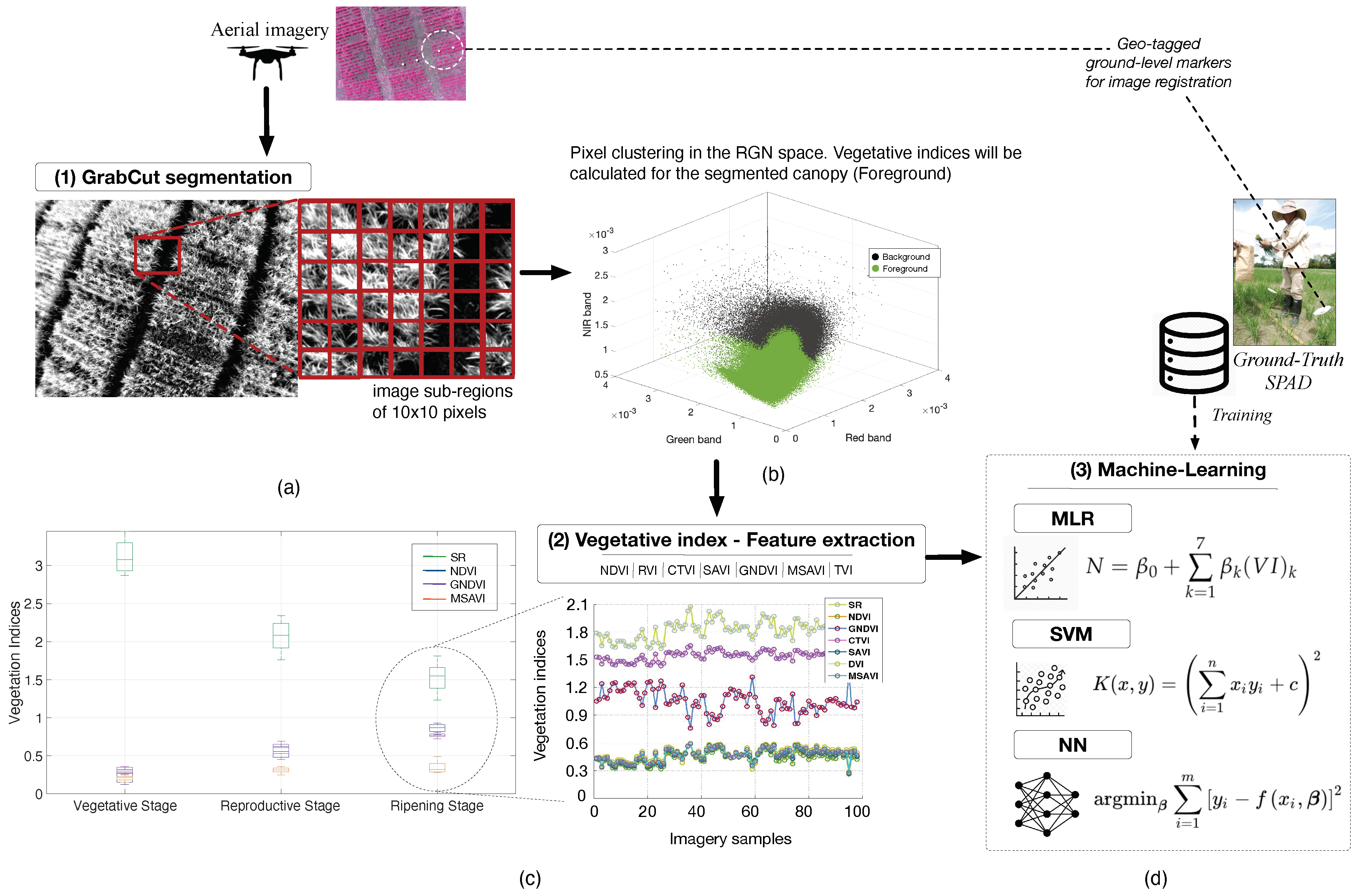
Figure 5 details the procedure required by the machine-learning models. After registration, images are segmented by using the proposed GrabCut method. Although all pixels in the image are evaluated in Algorithm 2, we use pixel clusters of 10 × 10 to calculate the VI formulas, as shown in 
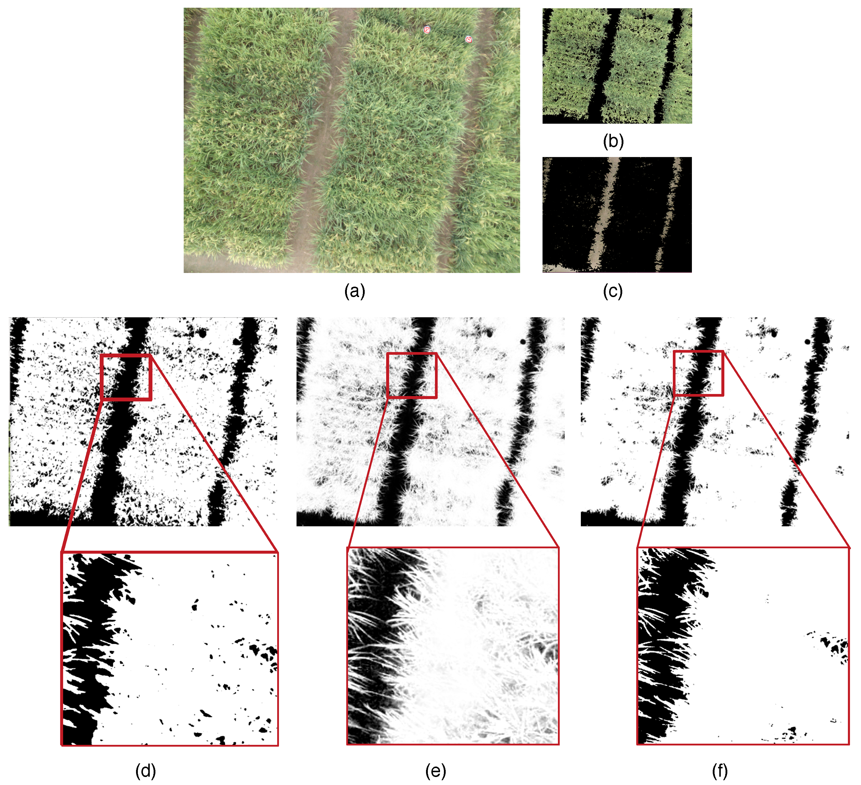
Figure 5a. After segmentation, pixels representing the rice canopy are separated from the background, as shown in Figure 5b. All vegetation indices are calculated as the average within each image sub-region.
At canopy-level, several factors affect the spectral reflectances of the crop: solar radiation and weather conditions, plant morphology and color, leaf angles, undergrowth, soil characteristics, and ground water layers. As mentioned in Section 2.1, the multispectral camera comes with an integrated sunshine sensor to compensate light variations in the resultant image. In addition, the GrabCut segmentation method deals with the filtering of undergrowth and other soil noises. Despite that, it remains crucial to validate the accuracy of the selected VIs, since the estimation of N depends on the accuracy and reliability of the extracted features. In this regard, Figure 5c presents several VI calculations in order to analyze the variance of the VI features through the entire phenological cycle of the crop. For this test, we calculated the VI formulas from 360 random images per crop stage under different environmental conditions. We show the most representative VIs to nitrogen variations: simple ratio (SR), normalized difference vegetation index (NDVI), green normalized difference vegetation index (GNDVI), and soil-adjusted vegetation index (MSAVI). As observed, the low variance exhibited through the entire phenological cycle allows us to use the VI features as inputs to the ML models detailed in Figure 5d.

3. Results

The experiments reported in this paper were carried out during 2018 in the rice farms of the Center of International Agriculture (CIAT). Trials were conducted during the dry season (June-September), as detailed in Table 1. We conducted 3 trials per crop stage (vegetative, reproductive, and ripening).

3.1. UAV Control Results

Figure 6 shows simulation results to evaluate the performance of the proposed controller in terms of wind-disturbance rejection. In plot (a), the desired trajectory (red line) was defined for the UAV to cover the crop while following the trapezoidal velocity profile shown in plot (b). This trajectory profile enables the UAV to hover at certain points (black dots) to capture aerial images. The maximum UAV velocity was set to 1.5 ms 1 .
In plot (a), a wind disturbance ( V w i n g = 9 ms 1 ) was added at the starting point of the trajectory, causing the UAV to mismatch the desired path (the V w i n g vector was applied onto the y + direction). The response of the UAV driven by the BS-DAF attitude controller corresponds to the black line, whereas the PID controller is the green line. As observed, the BS + DAF immediately counteracted the disturbance by generating the corresponding roll command ϕ depicted in plot (d). This response allowed the UAV to follow the path precisely, maintaining the position error along the y axis near to zero, as shown in plot (c). Under this scenario, our system obtained a maximum tracking error of 2 % .
A second wind disturbance was added when the UAV reached 10 m in altitude. In this case, V w i n g  was applied onto the z-direction (z points downwards). As observed, an augmented thrust caused a large altitude tracking error that affected the UAV for both control schemes similarly. Unlike for roll and pitch, the BS+DAF control does not drive the altitude loop. In general, the UAV was able to position in the hovering knot-points accurately (black dots in plot a), maintaining a minimum error with the GPS waypoints. For the rest of the trajectory, the results demonstrate that the backstepping + DAF is accurate and reliable to reject external wind disturbances.

3.2. Image Segmentation Results

Algorithms 1 and 2 are applied for each input image in an iterative manner. In Figure 7a, two markers placed as geo-referenced guiding points appear in the RGB image (red dots in the top-right corner). The algorithm provides to the user with the option to manually select these points in order to remove them from the segmentation process. An example of semi-manual GrabCut segmentation with minimal user interaction is shown in Figure 7d. If those points are not manually removed, the corresponding pixels will be classified either in the background of foreground cluster automatically. Subsequently, plots (b) and (c) show how the initial foreground and background are defined. Plot (d) shows an example of applying Algorithm 1 to the input image from (a), whereas plot (e) shows the results when combining the GrabCut with the guided-filter (GF) approach, yielding an automatic segmentation process, as detailed in Algorithm 2. As shown in plot (e), the GF refinement achieves richer detail in the final segmentation. This result can be compared against a traditional Otsu’s threshold method shown in plot (f). Although the results from Figure 7e are promising, we implemented a final refinement process based on the so-called GF feathering filtering, in which Algorithm 2 is used with a carefully selected radius r and regularization parameter ϵ . The GF feathering filtering enables a faster implementation of Algorithm 2 by avoiding the O ( N 2 ) computational restriction of the convolution.
The quality of the proposed segmentation method was tested and compared against the binary mask segmentation of three well-known methods: (i) k-means [49], (ii) mean-shift [50], and (iii) manual threshold over the HSV color representation [51]. The acronyms used in the comparison results are listed in Table 4. By applying the fully automatic segmentation method described in Algorithm 2, we used the precision, recall, and the F1-score to measure the performance of the proposed segmentation listed as GCFauto in Table 4. Figure 8 and Table 5 show the results.
For image pre-processing, the automatic GrabCut method in Algorithm 2 with the guided-filter refinement enabled precise plot segmentation of multispectral imagery with richer detail of the canopy structure and proper elimination of the background cluster. In this regard, Figure 9 shows the final segmentation results. In plot (a), the segmented image is achieved by combining the multispectral image shown in plot (b) and the RGB images from plot (c). In plot (d), the values for the radius and ϵ depend on the image size. For this application, those values were experimentally determined as r = 60 and ϵ = 0.001 2 . Without this segmentation method, significant image corrections would be needed.

3.3. Nitrogen Estimations

In the following, we present a comprehensive comparison among multi-variable linear regressions (MLR), support vector machines (SVM), and artificial neural networks (NN) for the estimation of the canopy N. All these models were trained using the ground-truth (cf. Table 2) containing the direct measurements of leaf chlorophyll based on SPAD readings. In this regard, the estimation results are all given in SPAD scale, in which the linear relationship with nitrogen is defined as: N = 0.079 ( S P A D ) 0.154 , according to the work reported in [37].

3.3.1. MLR Models

Figure 10 shows the estimation results using the MLR. The samples-axis corresponds to the aerial imagery used for the estimation of nitrogen thought the phenological cycle. As previously mentioned, direct SPAD measurements were conducted for selected crop plots in order to assemble the ground-truth dataset. Given that, our system selects those aerial samples matching with the GPS coordinates of the ground measurements. Overall, the MLR achieved an average N correlations of 0.93 (V), 0.89 (V), and 0.82 (Ri). The data was filtered using a Moving Average Filter to reduce signal fluctuations and smooth the estimation result. Table 6 details the numerical data. Since the coefficients for the linear regressions were found and calibrated for each stage independently, we found strong linear relationships in the vegetative stage between the VIs and the N accumulation. Through the ripening stage, the yellow color becomes predominant and parcels cannot be distinguished with ease (as shown in Figure 2c). This changes in the canopy color and dense biomass accumulation tend to saturate the linear relationships between the VIs and the canopy reflectances.

3.3.2. SVM Models

We first tried to find a single SVM model for the entire crop phenological cycle; however, the canopy reflectances and the VIs changed drastically from vegetative through ripening. In this regard, an SVM model was defined for each crop stage independently, as shown in Table 7. In addition, Figure 11 details the estimation results for the N dynamics. Based on these results, the following SVM configurations are selected for our estimation system:
  • Vegetative: Quadratic, correlation = 0.96, RMSE = 2.34, R 2 = 0.927, ϵ = 2 .
  • Reproductive: Quadratic, correlation = 0.94, RMSE = 2.33, R 2 = 0.892, ϵ = 2 .
  • Ripening: Quadratic, correlation = 0.87, RMSE = 2.04, R 2 = 0.77, ϵ = 0.5 .

3.3.3. NN Models

Neural networks (NN) with several hidden layers and optimization algorithms were tested. We highlight the results with two and five hidden layers. In Figure 12, the NN with two layers achieved a correlation = 0.964, RSME = 3.315, and  R 2 = 0.94. Increasing up to five layers, the NN achieved a correlation = 0.986, RSME = 1.703, and R 2 = 0.97. Several training functions were tested for each crop stage, where the BFGS Quasi-Newton functions achieved accurate results for most of the vegetative stages, whereas the Levenberg–Marquardt function for both reproductive and ripening. The numerical data are reported in Table 8. Based on the results, the following NN configurations are selected for our estimation system:
  • Vegetative: BFGS Quasi-Newton, correlation = 0.986, RMSE = 1.643, R 2 = 0.972.
  • Reproductive: Levenberg-Marquardt, correlation = 0.944, RMSE = 3, R 2 = 0.891.
  • Ripening: Levenberg-Marquardt, correlation = 0.890, RMSE = 1.835, R 2 = 0.792.

3.3.4. Machine-Learning Comparative Results

Figure 13 shows overall N estimation results obtained for each machine learning model. In general, we demonstrated strong correlations between the canopy N and the corresponding vegetative indices. In the case of MLR models, the coefficients for the regressions were determined and independently calibrated for each crop stage. We encountered that the N dynamics have strong linear dependencies with MSAVI, GNDVI, and NDVI; concretely, during vegetative and reproductive stages. Table 9 reports the overall numerical data.
From the ROC curve reported in Figure 13d, the accuracy (ACC) was calculated for each ML model. Neural networks achieved an average ACC = 0.85, improving the estimations of canopy N over the other ML models. In fact, by comparing the N-to-SPAD correlations reported on Table 9, the correlation metric was improved over each crop stage. Table 9 compares the mean N estimations achieved by each ML method against the mean SPAD-based N readings measured at ground level. Mean results are presented for each crop stage: vegetative (V), reproductive (R), and ripening (Ri). The last columns in Table 9 report the mean linear correlations between estimations and measurements.
By comparing the neural networks (NN) against the multi-variable linear regressions (MLR) and support vector machines (SVM), the former estimator achieves higher correlations partly due to the reliability and size of the assembled ground-truth database for training, i.e., reliable N datasets (direct N-leaf measurements) with sufficient variations of the crops during the growth stage (see the experimental protocol in Section 2). In addition, some VIs, such as the simple ratio (SR), tend to saturate as long the the crop grows, but other vegetative indices that behave better with higher biomass and N concentration compensate the effect of the saturated ones. The nonlinear combinations of these VIs enable the NN to achieve accurate estimations.
Furthermore, we tested the effects of the UAV control architecture proposed in Section 2.3, for improving the N estimations by means of precise position tracking during flight. Figure 14 presents the results. Plot (b) shows the X-Y tracking trajectory for each flight control scenario. The UAV was flying at a constant altitude reference of 20 m over the crop at a maximum speed of 1.5 m/s. The black boxes represent the crop plots with ground-level markers where direct N measurements were taken via SPAD. The green dotted circles show the points where the UAV stops and hovers during 4 s to capture canopy imagery.
The paths followed by the UAV are shown for both controllers; one driven by the PID that comes standard with the UAV autopilot, and the other driven by the proposed BS+DAF. Likewise, the star markers represent the GPS points of the images taken while hovering (black color for the PID and red for the BS + DAF). As observed, the attitude stabilization of the UAV seems to be more affected with the PID, since the aerial samples within each hovering area (black star markers) are spread over different positions. Instead, the aerial samples obtained with the BS + DAF (red star markers) tend to be more concentrated within the crop plot of interest. The goal is actually capturing most images in the GPS coordinates that accurately matches with the GPS position of the white markers at ground-level, as depicted in Figure 14a.
Finally, Figure 14c presents the N estimation results achieved under both control flight scenarios. Larger fluctuations, noise, and estimation errors are presented when the ML methods are trained and tested with the imagery dataset captured by the PID-driven UAV. This is mainly due to the imprecise X-Y positioning of the aerial vehicle during hovering (caused by improper attitude stabilization), in which several images capture crop areas that do not necessarily match with the ground-level markers, as detailed in Figure 14b. On the other hand, the proposed BS+DAF controller demonstrated being suitable for the proper regulation of the angular motions of the UAV by compensating external disturbances faster and achieving accurate X-Y positioning. As a result, The N estimations correlate higher with the ground-truth. As shown in the histograms in Figure 14d, the N-to-SPAD correlations grouped higher for the experiments driven by the proposed BS+DAF controller.

4. Discussion

The results presented in this work demonstrate a significant improvement in leaf nitrogen prediction in rice crops from images obtained via UAVs, validated with high SPAD correlations. These results are thanks to a combination of technological contributions, namely: (i) a novel UAV stabilization control scheme named BS+DAF that enables precise multispectral aerial image acquisition and registration with ground-truth fiducials, even in the presence of strong wind perturbations, (ii) an automated GrabCut image segmentation method, which leads to finer detail of the plant’s canopy in the RGN space, as detailed in Figure 5b and Figure 9d, and (iii) the successful application of machine learning methods trained with the vegetation indices (VI) extracted from the segmented multispectral imagery. Figure 5c confirms the increased reliability and accuracy per VI by calculating the data variance at each crop stage.
In a similar manner, Table 9 summarizes the higher nitrogen-to-SPAD correlations achieved with the implemented neural networks, and confirms the significant nonlinear relationships between leaf spectral reflectances (VI) and chlorophyll-based estimated N concentrations. These N estimation results are comparable to other state-of-the-art results presented in the scientific literature. In [52], Figure 7b shows N estimations in rice using linear regression models, for which the authors report: R M S E = 0.212 , correlation r = 0.89 , and R 2 = 0.803 . Our results (tabulated in Table 8 and Table 9) reach mean correlations for the vegetative stage ( r = 0.986 ), reproductive ( r = 0.9442 ), and ripening stage ( r = 0.89 ). In [53], Table 6 and Figure 5 present N-status estimations in rice using vegetation indices calculated with aerial UAV imagery. Authors compared several regression models, with a highest R 2 of 0.74 using the LDM method. In our case, Table 8 lists higher R 2 values from the Levenberg–Marquardt method.
Our approach contributes novel solutions to commercial UAV-based phenotyping technologies, particularly to image-based remote sensing applications that adopt photogrammetric geometric image post-processing methods for image correction, and enables crop/plot analysis in real-time.
One important drawback of our solution was the estimation of canopy N for crops with higher biomass. Counter to the expectation of finding a higher N correlation as a function of crop growth, the correlation results decreased in the ripening stage, as depicted in Figure 13e and from the numerical data presented in Table 9. We attribute this to the disproportionately high number of senescent leaves (yellow color with a bandwidth of 570–590 nm) that do not properly match with the VI dominant wavelengths (see Table 3). Consequently, we suggest introducing plant senescence reflectance as an added variable for the discovery of novel vegetative indices to enhance our system.

5. Conclusions

This paper presents an integrated UAV system with non-invasive image-based methods for the estimation and monitoring of the N dynamics in rice crops. Several challenges were addressed, associated with image segmentation and UAV navigation control, to achieve reliable machine learning training and highly correlated results to SPAD. The proposed BS+DAF attitude controller led to precise UAV way-point tracking, with position errors below 2 % . This was key to capture aerial multispectral imagery during hovering that accurately matched with the GPS positions of the SPAD measurements at ground-level. This reduces the need for computationally expensive photogrammetry methods.
Higher N correlations were achieved with neural networks: 0.98 in the vegetative stage, 0.94  in reproductive, and 0.89 in ripening, with an ROC accuracy of 0.85 . This is a promising result towards the autonomous estimation of rice canopy nitrogen in real-time. With the advent of small AI-dedicated systems on chip (SoC) and the powerful computing capabilities of our UAV system, we expect upcoming work to achieve real-time computation of the machine learning methods presented in this work.
Several challenges still remain for improving the N estimations, especially when the crop biomass is high. Rice crops commonly have several mixed varieties per small plot areas. Therefore, besides the assessment of the N dynamics as a function of the crop stages, it is also crucial to identify and classify the plants according to their genotype, given that nitrogen is highly sensitive to plant oxygen consumption, root growth, among other variables. To this purpose, the aerial identification of different plant varieties requires sensing spatial resolutions below 30 cm. In addition, high-dimensional data clustering is needed for the extraction of relevant features according to the plant variety.

Supplementary Materials

The following are available online at https://0-www-mdpi-com.brum.beds.ac.uk/2072-4292/12/20/3396/s1, FILE S1: RAW data supporting image segmentation metrics, multispectral imagery imagery used for machine learning testing, and nitrogen estimation results are available at the Open Science Framework: https://osf.io/cde6h/?view_only=1c4e5e03b9a34d3b96736ad8ab1b2774. FILE S2: Experimental protocol for crop monitoring available at https://www.protocols.io/view/protocol-bjxskpne. VIDEO S3: The video is available in the online version of this article. The video accompanying this paper illustrates the steps performed during the experiments.

Author Contributions

Conceptualization, J.D.C., N.C.-B., F.C., and J.S.C.; methodology, J.D.C., M.C.R., F.C., and A.J.-B.; software, N.C.-B., J.S.C., and D.C.; validation, J.D.C., I.F.M., E.P., D.C., N.C.-B., and J.S.C.; formal analysis and investigation, J.D.C., M.C.R., E.P., F.C., I.F.M., and A.J.-B.; data curation, E.P.; writing—original draft preparation, J.D.C. and F.C.; writing—review and editing, A.J.-B., I.F.M., and M.C.R.; supervision, A.J.-B. and J.D.C. All authors have read and agreed to the published version of the manuscript.

Funding

This work was funded by the OMICAS program: Optimización Multiescala In-silico de Cultivos Agrícolas Sostenibles (Infraestructura y validación en Arroz y Caña de Azúcar), anchored at the Pontificia Universidad Javeriana in Cali and funded within the Colombian Scientific Ecosystem by The World Bank, the Colombian Ministry of Science, Technology and Innovation, the Colombian Ministry of Education and the Colombian Ministry of Industry and Turism, and ICETEX under GRANT ID: FP44842-217-2018.

Acknowledgments

The authors would like to thank all CIAT staff that supported the experiments over the crops located at CIAT headquarters in Palmira, Valle del Cauca, Colombia; in particular to Yolima Ospina and Cecile Grenier for their support in upland and lowland trials. Also, to Carlos Devia from Javeriana University for the insights regarding the structuring of the datasets.

Conflicts of Interest

The authors declare no conflict of interest.

Appendix A. UAV Equations of Motion

Equations of motion (EoM) that describe the inertial and aerodynamics effects are introduced, including a six-dimensional operator describing the spatial accelerations of the body frame as a function of the UAV inertias, moments, and aerodynamics. Second, we introduce a nonlinear MPC-based controller to regulate the stabilization of the UAV, specifically both pitch θ and roll ϕ angles, under external force perturbations.
Our UAV is a Vertical Takeoff and Landing (VTOL) four-rotor drone. As shown in Figure A1a, the body frame { b } is a six degree of freedom rigid body. Rotations about the body-frame axes are designated by the Euler angles: roll ( ϕ ), pitch ( θ ), and yaw ( ψ ) following standard aerodynamic conventions. In this sense, the 6D spatial acceleration V ˙ b 6 x 1 of the body frame can be written as:
V ˙ b = ω ˙ b υ ˙ b = ϕ ¨ θ ¨ ψ ¨ x ¨ b y ¨ b z ¨ b
Figure A1. Physical parameters used for UAV modeling and control. (a) Equations of motion are derived using three frames of reference: the inertial frame { i } , the body frame { b } located at the center of mass, and the rotors frame { o i } , o i : 1 4 . Each rotor generates a vertical thrust ( T o i ) that depends on the rotor angular speed ( ω o i ) and the geometrical properties of the propeller blades. (b) Blade properties for deriving aerodynamics equations. We used Blade-Element-Theory computation to calculate both lift and drag coefficients using the FoilSim III simulator provided by NASA [54]. Our UAV has a lift coefficient of C L = 1.6 and a drag coefficient of C D = 0.042 , since l / r = 0.7 .
Remotesensing 12 03396 g0a1
Both rotational ω ˙ and translational υ ˙ accelerations could be derived from the Newton–Euler formulation, as:
V ˙ b = I b 1 [ F b I ˙ b V b ] ,
being I b 6 x 6 the spatial inertia operator calculated at the Center of Mass (CM) of the body frame { b } . It can be expressed as:
I b = J b 0 0 m U = I x x I x y I x z 0 0 0 I x y I y y I y z 0 0 0 I x z I y z I z z 0 0 0 0 0 0 m 0 0 0 0 0 0 m 0 0 0 0 0 0 m ,
where J b 3 x 3 is the inertial tensor with d i a g ( I x x , I y y , I z z ) being the moments of inertia, m is the mass of the UAV, and U is a 3 × 3 identity operator. Likewise, the term F b 6 x 1 in Equation (A2) is the 6D spatial force acting on the CM of { b } . F b contains the effects caused by both inertial ( N b ) and aerodynamics ( T b ) forces acting on the body frame:
F b = N b f b = ( N b , x ) + ( τ ϕ ) ( N b , y ) + ( τ θ ) ( N b , z ) + ( τ ψ ) f b , x f b , y f b , z = ( θ ˙ ψ ˙ I y y I z z ) + s o i , b j ^ ( T 4 T 3 ) ( ϕ ˙ ψ ˙ I z z I x x ) + s o i , b i ^ ( T 1 T 2 ) ( θ ˙ ϕ ˙ I x x I y y ) + ( T 3 + T 4 T 1 T 2 ) s ψ s ϕ + c ψ s θ c ϕ T b c ψ s ϕ + s ψ s θ c ϕ T b m g ( c ψ c ϕ ) T b
In Equation (A4), we have determined an expression that incorporates the thrust produced by each independent rotor ( T o i ) o i : 1 4 . These aerodynamic terms govern the generation of rolling ( τ ϕ ), pitching ( τ θ ) and yawing ( τ ψ ) torques at the CM of the UAV, where the term s o i , b = 0.18 m is the distance between each rotor to the body frame (see Figure A1a). In addition, T o i depends on the lift (L) and drag (D) forces acting on each propeller, as shown in Figure A1b. It can be written as:
T o i = L + D = 1 2 ρ a i r ω o i 2 A p r o p C L + C D ,
where ρ a i r = 1.20 Kgm 3 is the density of air, ω o i , o i : 1 4 is the rotor speed, A p r o p = 0.013   m 2 is the propeller transversal area, C L is the lift coefficient, and C D is the drag coefficient. As shown in Figure A1b, we have estimated both values as C L = 1.6 and C D = 0.042 , respectively. In this sense, the net vertical thrust ( T b ) generated at the CM of the UAV can be calculated as:
T b = o i = 1 4 T o i
As observed in Equation (A4), T b governs the generation of the linear forces. The expressions s ψ , c ψ denote s i n ( ψ ) and c o s ( ψ ) , respectively. Finally, the term m = 0.43   K g is the mass of the UAV and g = 9.81   m s 2 is the gravitational acceleration. In the forthcoming section, we will derive the control strategy to regulate the angular motions precisely. Since our control approach will depend on the UAV model, we introduce the computational steps to calculate the EoM in Algorithm A1.   
Algorithm A1: EoM Computation.
  • Step 1: Aerodynamic forces
  • Read the rotors speed from encoders: ω o i , o i : 1 4
  • Calculate both lift and drag forces acting on each propeller:
  • L 1 2 C L ρ a i r ω o i 2 A p r o p ,
  • D 1 2 C D ρ a i r ω o i 2 A p r o p
  • Calculate the thrust produced by each rotor: T o i = L + D o i : 1 4
  • Calculate net thrust produced at CM: T b = o i = 1 4 T o i
  • Rotational forces (rolling, pitching, and yawing) torques onto the body frame:
  • τ ϕ s o i , c m j ^ T 4 T 3
  • τ θ s o i , c m i ^ T 1 T 2
  • τ ψ τ 3 + τ 4 τ 1 τ 2
  • Linear forces acting onto the body frame:
  • f b , x s ψ s ϕ + c ψ s θ c ϕ T b
  • f b , y c ψ s ϕ + s ψ s θ c ϕ T b
  • f b , z ( c ψ c ϕ ) T b
  • 6D Aerodynamic Forces: [ τ ϕ τ θ τ ψ f b , x f b , y f b , z ] T
  • Step 2: Inertial forces
  • Calculate 6D inertial operator: I b = J b 0 0 m U
  • Calculate inertial terms:
  • N b , x θ ˙ ψ ˙ I y y I z z
  • N b , y ϕ ˙ ψ ˙ I z z I x x
  • N b , z θ ˙ ϕ ˙ I x x I y y
  • f b , z m g c o s ( ψ ) c o s ( ϕ ) T b
  • Calculate 6D Forces: F b [ N b , x + τ ϕ N b , y + τ θ N b , z + τ ψ f b , x f b , y f b , z ] T
  • Step 3: 6D Equations of Motion (EoM)
  • V ˙ b I b 1 [ F b I ˙ b V b ]
  • Return V ˙ b

Appendix B. Backstepping + DAF Control Derivation

The proposed control law has to be sensitive to small changes in both angular motions, therefore, an error dynamics could be defined as a function of the angular rates, as:
e ˙ ϕ = ϕ ˙ d ω x , e ˙ θ = θ ˙ d ω y
In Equation (A7), both ω x and ω y are measured by the IMU sensor onboard the UAV. The goal is to obtain a desired angular acceleration terms within the control law to account for small angular rate changes. These terms are called desired acceleration function (DAF):
ϕ ¨ d = f ( ϕ , ϕ ˙ , F b ) = 1 0 0 0 0 0 V ˙ b , θ ¨ d = f ( θ , θ ˙ , F b ) = 0 1 0 0 0 0 V ˙ b
Both DAF terms ϕ ¨ d and θ ¨ d are extracted from the spatial acceleration V ˙ b 6 x 1 computed in Algorithm A1. To make explicit the DAF terms from Equation (A8) within the backstepping, in the following we focus on deriving the control law for roll ( u ϕ ).
From Equation (A6), we introduce a virtual control law that governs the error dynamics, yielding a second tracking error e 2 = ω x d ω x where ϕ ˙ d ω x d . In this sense, a proportional-derivative-integral structure is defined for the virtual control law ω x d , as:
ω x d = k p e ϕ + ϕ ˙ d + k i e ϕ ( t ) d t ,
where K p and K i must be positive constants, since the BS requires a positive definite Lyapunov function (L) for stabilizing the tracking error: L e ϕ = e ϕ 2 2 . Now, replacing Equation (A9) into the virtual control error e 2 yields:
e 2 = ω x d ω x = k p e ϕ + ϕ ˙ d + k i e ϕ ( t ) d t ω x
By following the same approach from Equation (A7), the error dynamics for e ˙ 2 is determined as:
e ˙ 2 = k p e ˙ ϕ + ϕ ¨ d + k i e ϕ ω ˙ x
In Equation (A11), we have derived ϕ ¨ d corresponding to the DAF term for roll (see Equation (A8)). In this regard, the computation of Algorithm A1 is required to close the attitude loop. Now, the control action u ϕ is determined as:
u ϕ τ ϕ = I x x ϕ ¨ , ϕ ¨ ω ˙ x = I x x 1 τ ϕ
Replacing ω ˙ x from Equation (A12) in (A11) and isolating the control action, yields:
u ϕ = I x x [ k p e ˙ ϕ + ϕ ¨ d + k i e ϕ e ˙ 2 ]
Since the calculation of e ˙ ϕ and e ˙ 2 for the real system would introduce accumulative numerical errors, we need to rewrite the control law to be dependent of the tracking errors: e ϕ and e 2 . By isolating ω x = ω x d e 2 from Equation (A10) and replacing it into Equation (A7):
e ˙ ϕ = ϕ ˙ d ( ω x d e 2 )
Replacing Equation (A14) into (A13):
u ϕ = I x x [ k p ( ϕ ˙ d ω x d + e 2 ) + ϕ ¨ d + k i e ϕ e ˙ 2 ] ,
and replacing ω x d from Equation (A9):
u ϕ = I x x [ k p ( ϕ ˙ d ( k p e ϕ + ϕ ˙ d + k i e ϕ ) + e 2 ) + ϕ ¨ d + k i e ϕ e ˙ 2 ] = I x x [ k p ( e 2 k p e ϕ k i e ϕ ) + ϕ ¨ d + k i e ϕ e ˙ 2 ]
Finally, the expression for e ˙ 2 can be rewritten to follow the same form of e ˙ ϕ in Equation (A14). Likewise, ω x d is also replaced by Equation (A9):
Remotesensing 12 03396 i001
In Equation (A17), the integration of the error can be eliminated since the control law in Equation (A16) already ensures zero steady-state error for e ϕ . Replacing e ˙ 2 = e 2 k p e ϕ in Equation (A16):
u ϕ = I x x [ k p ( e 2 k p e ϕ k i e ϕ ) + ϕ ¨ d + k i e ϕ e 2 + k p e ϕ ] = I x x [ e ϕ ( k p k i k p 2 ) + e 2 ( k p 1 ) k p k i e ϕ + ϕ ¨ d ]
Equation (A18) presents the control law to regulate ϕ . This controller allows zero steady-state error for roll via e ϕ , it is sensitive to small variations in roll rate via e 2 , and it directly depends on the UAV model via the DAF term ϕ ¨ d (Algorithm A1). By following the same structure in Equation (A18), the control law to regulate the pitch angular motion ( θ ) is:
u θ = I y y [ e θ ( k p , 2 k i , 2 k p , 2 2 ) + e 2 ( k p , 2 1 ) k p , 2 k i , 2 e θ + θ ¨ d ]

References

  1. Zhang, K.; Liu, X.; Tahir Ata-Ul-Karim, S.; Lu, J.; Krienke, B.; Li, S.; Cao, Q.; Zhu, Y.; Cao, W.; Tian, Y. Development of Chlorophyll-Meter-Index-Based Dynamic Models for Evaluation of High-Yield Japonica Rice Production in Yangtze River Reaches. Agronomy 2019, 9, 106. [Google Scholar] [CrossRef] [Green Version]
  2. Yang, H.; Yang, J.; Lv, Y.; He, J. SPAD Values and Nitrogen Nutrition Index for the Evaluation of Rice Nitrogen Status. Plant Prod. Sci. 2014, 17, 81–92. [Google Scholar] [CrossRef]
  3. Dong, Z.; Wu, L.; Chai, J.; Zhu, Y.; Chen, Y.; Zhu, Y. Effects of Nitrogen Application Rates on Rice Grain Yield, Nitrogen-Use Efficiency, and Water Quality in Paddy Field. Commun. Soil Sci. Plant Anal. 2015, 46, 1579–1594. [Google Scholar] [CrossRef]
  4. Xu, G.; Fan, X.; Miller, A.J. Plant nitrogen assimilation and use efficiency. Annu. Rev. Plant Biol. 2012, 63, 153–182. [Google Scholar] [CrossRef] [PubMed] [Green Version]
  5. Nigon, T.J.; Yang, C.; Dias Paiao, G.; Mulla, D.J.; Knight, J.F.; Fernández, F.G. Prediction of Early Season Nitrogen Uptake in Maize Using High-Resolution Aerial Hyperspectral Imagery. Remote Sens. 2020, 12, 1234. [Google Scholar] [CrossRef] [Green Version]
  6. Wan, L.; Li, Y.; Cen, H.; Zhu, J.; Yin, W.; Wu, W.; Zhu, H.; Sun, D.; Zhou, W.; He, Y. Combining UAV-Based Vegetation Indices and Image Classification to Estimate Flower Number in Oilseed Rape. Remote Sens. 2018, 10, 1484. [Google Scholar] [CrossRef] [Green Version]
  7. Zhang, D.; Zhou, X.; Zhang, J.; Lan, Y.; Xu, C.; Liang, D. Detection of rice sheath blight using an unmanned aerial system with high-resolution color and multispectral imaging. PLoS ONE 2018, 13. [Google Scholar] [CrossRef] [PubMed] [Green Version]
  8. Liu, Y.; Cheng, T.; Zhu, Y.; Tian, Y.; Cao, W.; Yao, X.; Wang, N. Comparative analysis of vegetation indices, non-parametric and physical retrieval methods for monitoring nitrogen in wheat using UAV-based multispectral imagery. In Proceedings of the 2016 IEEE International Geoscience and Remote Sensing Symposium (IGARSS), Beijing, China, 10–15 July 2016; pp. 7362–7365. [Google Scholar] [CrossRef]
  9. Guan, S.; Fukami, K.; Matsunaka, H.; Okami, M.; Tanaka, R.; Nakano, H.; Sakai, T.; Nakano, K.; Ohdan, H.; Takahashi, K. Assessing Correlation of High-Resolution NDVI with Fertilizer Application Level and Yield of Rice and Wheat Crops Using Small UAVs. Remote Sens. 2019, 11, 112. [Google Scholar] [CrossRef] [Green Version]
  10. Mishra, P.; Asaari, M.S.M.; Herrero-Langreo, A.; Lohumi, S.; Diezma, B.; Scheunders, P. Close range hyperspectral imaging of plants: A review. Biosyst. Eng. 2017, 164, 49–67. [Google Scholar] [CrossRef]
  11. Bergstrasser, S.; Fanourakis, D.; Schmittgen, S.; Cendrero-Mateo, M.P.; Jansen, M.; Rascher, H.S.U. HyperART: Non-invasive quantification of leaf traits using hyperspectral absorption-reflectance-transmittance imaging. Plant Methods 2015, 11, 1. [Google Scholar] [CrossRef] [Green Version]
  12. Pandey, P.; Ge, Y.; Stoerger, V.; Schnable, J.C. High Throughput In vivo Analysis of Plant Leaf Chemical Properties Using Hyperspectral Imaging. Front. Plant Sci. 2017, 8, 1348. [Google Scholar] [CrossRef] [PubMed] [Green Version]
  13. Sun, D.; Cen, H.; Weng, H.; Wan, L.; Abdalla, A.; El-Manawy, A.I.; Zhu, Y.; Zhao, N.; Fu, H.; Tang, J.; et al. Using hyperspectral analysis as a potential high throughput phenotyping tool in GWAS for protein content of rice quality. Plant Methods 2019, 15, 54. [Google Scholar] [CrossRef] [PubMed]
  14. Lu, J.; Yang, T.; Su, X.; Qi, H.; Yao, X.; Cheng, T.; Zhu, Y.; Cao, W.; Tian, Y. Monitoring leaf potassium content using hyperspectral vegetation indices in rice leaves. Precis. Agric. 2020, 21, 324–348. [Google Scholar] [CrossRef]
  15. Wang, W.; Yao, X.; Tian, Y.-C.; Liu, X.-J.; Ni, J.; Cao, W.-X.; Zhu, Y. Common Spectral Bands and Optimum Vegetation Indices for Monitoring Leaf Nitrogen Accumulation in Rice and Wheat. J. Integr. Agric. 2012, 11, 2001–2012. [Google Scholar] [CrossRef]
  16. Sun, J.; Yang, J.; Shi, S.; Chen, B.; Du, L.; Gong, W.; Song, S. Estimating Rice Leaf Nitrogen Concentration: Influence of Regression Algorithms Based on Passive and Active Leaf Reflectance. Remote Sens. 2017, 9, 951. [Google Scholar] [CrossRef] [Green Version]
  17. Singh, A.K.; Ganapathysubramanian, B.; Sarkar, S.; Singh, A. Deep Learning for Plant Stress Phenotyping: Trends and Future Perspectives. Trends Plant Sci. 2018, 23, 883–898. [Google Scholar] [CrossRef] [Green Version]
  18. Xiong, X.; Duan, L.; Liu, L.; Tu, H.; Yang, P.; Wu, D.; Chen, G.; Xiong, L.; Yang, W.; Liu, Q. Panicle-SEG: A robust image segmentation method for rice panicles in the field based on deep learning and superpixel optimization. Plant Methods 2017, 13, 104. [Google Scholar] [CrossRef] [Green Version]
  19. Ubbens, J.R.; Stavness, I. Deep Plant Phenomics: A Deep Learning Platform for Complex Plant Phenotyping Tasks. Front. Plant Sci. 2017, 8, 1190. [Google Scholar] [CrossRef] [Green Version]
  20. Ghosal, S.; Blystone, D.; Singh, A.K.; Ganapathysubramanian, B.; Singh, A.; Sarkar, S. An explainable deep machine vision framework for plant stress phenotyping. Proc. Natl. Acad. Sci. USA 2018, 115, 4613–4618. [Google Scholar] [CrossRef] [Green Version]
  21. Tilly, N.; Aasen, H.; Bareth, G. Fusion of Plant Height and Vegetation Indices for the Estimation of Barley Biomass. Remote Sens. 2015, 7, 11449–11480. [Google Scholar] [CrossRef] [Green Version]
  22. Wang, C.; Nie, S.; Xi, X.; Luo, S.; Sun, X. Estimating the Biomass of Maize with Hyperspectral and LiDAR Data. Remote Sens. 2016, 9, 11. [Google Scholar] [CrossRef] [Green Version]
  23. Wang, Y.; Zhang, Z.; Feng, L.; Du, Q.; Runge, T. Combining Multi-Source Data and Machine Learning Approaches to Predict Winter Wheat Yield in the Conterminous United States. Remote Sens. 2020, 12, 1232. [Google Scholar] [CrossRef] [Green Version]
  24. Yang, Z.; Shen, D.; Yap, P.T. Image mosaicking using SURF features of line segments. PLoS ONE 2017, 12. [Google Scholar] [CrossRef] [PubMed] [Green Version]
  25. Caruso, G.; Zarco-Tejada, P.J.; González-Dugo, V.; Moriondo, M.; Tozzini, L.; Palai, G.; Rallo, G.; Hornero, A.; Primicerio, J.; Gucci, R. High-resolution imagery acquired from an unmanned platform to estimate biophysical and geometrical parameters of olive trees under different irrigation regimes. PLoS ONE 2019, 14, e0210804. [Google Scholar] [CrossRef] [PubMed] [Green Version]
  26. Bendig, J.; Bolten, A.; Bareth, G. UAV-based Imaging for Multi-Temporal, very high Resolution Crop Surface Models to monitor Crop Growth Variability. Photogramm. Fernerkund. Geoinf. 2013, 2013, 551–562. [Google Scholar] [CrossRef]
  27. Zhou, X.; Zheng, H.B.; Xu, X.Q.; He, J.Y.; Ge, X.K.; Yao, X.; Cheng, T.; Zhu, Y.; Cao, W.X.; Tian, Y.C. Predicting grain yield in rice using multi-temporal vegetation indices from UAV-based multispectral and digital imagery. ISPRS J. Photogramm. Remote Sens. 2017, 130, 246–355. [Google Scholar] [CrossRef]
  28. Han, Y.; Qin, R.; Huang, X. Assessment of dense image matchers for digital surface model generation using airborne and spaceborne images—An update. Photogram. Rec. 2020, 35, 58–80. [Google Scholar] [CrossRef]
  29. Comba, L.; Biglia, A.; Aimonino, D.R.; Gay, P. Unsupervised detection of vineyards by 3D point-cloud UAV photogrammetry for precision agriculture. Comput. Electron. Agric. 2018, 155, 84–95. [Google Scholar] [CrossRef]
  30. Maimaitijiang, M.; Sagan, V.; Sidike, P.; Maimaitiyiming, M.; Hartling, S.; Peterson, K.T.; Maw, M.J.W.; Shakoor, N.; Mockler, T.; Fritschid, F.B. Vegetation Index Weighted Canopy Volume Model (CVM VI ) for soybean biomass estimation from Unmanned Aerial System-based RGB imagery. ISPRS J. Photogramm. Remote Sens. 2019, 151, 27–41. [Google Scholar] [CrossRef]
  31. Sun, S.; Li, C.; Chee, P.W.; Paterson, A.H.; Jiang, Y.; Xu, R.; Robertson, J.S.; Adhikari, J.; Shehzad, T. Three-dimensional photogrammetric mapping of cotton bolls in situ based on point cloud segmentation and clustering. ISPRS J. Photogramm. Remote Sens. 2020, 160, 195–207. [Google Scholar] [CrossRef]
  32. Schirrmann, M.; Hamdorf, A.; Garz, A.; Ustyuzhanin, A.; Dammer, K.H. Estimating wheat biomass by combining image clustering with crop height. Comput. Electron. Agric. 2016, 121, 374–384. [Google Scholar] [CrossRef]
  33. Kandwal, R.; Kumar, A.; Bhargava, S. Existing Image Segmentation Techniques. Int. J. Adv. Res. Comput. Sci. Softw. Eng. 2014, 4, 2277–2285. [Google Scholar]
  34. Rother, C.; Kolmogorov, V.; Blake, A. “GrabCut”: Interactive foreground extraction using iterated graph cuts. ACM Trans. Graph. 2004, 23, 309–314. [Google Scholar] [CrossRef]
  35. Devia, C.A.; Rojas, J.P.; Petro, E.; Martinez, C.; Patino, D.; Rebolledo, M.C.; Colorado, J. High-Throughput Biomass Estimation in Rice Crops Using UAV Multispectral Imagery. J. Intell. Robot. Syst. 2019, 96, 573. [Google Scholar] [CrossRef]
  36. Assmann, J.J.; Kerby, J.T.; Cunliffe, A.M.; Myers-Smith, I.H. Vegetation monitoring using multispectral sensors—Best practices and lessons learned from high latitudes. J. Unmanned Veh. Syst. 2018, 334730. [Google Scholar] [CrossRef] [Green Version]
  37. Thaiparnit, S.; Ketcham, M. A Prediction Algorithm for Paddy Leaf Chlorophyll Using Colour Model Incorporate Multiple Linear Regression. Eng. J. 2017, 21, 269–280. [Google Scholar] [CrossRef] [Green Version]
  38. Kanke, Y.; Tubaña, B.; Dalen, M.; Harrell, D. Evaluation of red and red edge reflectance-based vegetation indices for rice biomass and grain yield prediction models in paddy fields. Precis. Agric. 2016, 17, 507–530. [Google Scholar] [CrossRef]
  39. Prabhakara, K.; Hively, W.; McCarty, G. Evaluating the relationship between biomass, percent groundcover and remote sensing indices across six winter cover crop fields in maryland, united states. Int. J. Appl. Earth Obs. Geoinf. 2015, 39, 88–102. [Google Scholar] [CrossRef] [Green Version]
  40. Gnyp, L.; Miao, Y.; Yuan, F.; Ustin, S.; Yu, K.; Yao, Y.; Huang, S.; Bareth, G. Hyperspectral canopy sensing of paddy rice aboveground biomass at different growth stages. Field Crops Res. 2014, 155, 42–55. [Google Scholar] [CrossRef]
  41. Cammarano, D.; Fitzgerald, G.J.; Casa, R.; Basso, B. Assessing the Robustness of Vegetation Indices to Estimate Wheat N in Mediterranean Environments. Remote Sens. 2014, 6, 2827–2844. [Google Scholar] [CrossRef] [Green Version]
  42. Naito, H.; Ogawa, S.; Valencia, M.; Mohri, H.; Urano, Y.; Hosoi, F.; Shimizu, Y.; Chavez, A.; Ishitani, M.; Selvaraj, M.; et al. Estimating rice yield related traits and quantitative trait loci analysis under different nitrogen treatments using a simple tower-based field phenotyping system with modified single-lens reflex cameras. J. Photogramm. Remote Sens. 2017, 135, 50–62. [Google Scholar] [CrossRef]
  43. Arai, K.; Sakashita, M.; Shigetomi, O.; Miura, Y. Estimation of Protein Content in Rice Crop and Nitrogen Content in Rice Leaves Through Regression Analysis with NDVI Derived from Camera Mounted Radio-Control Helicopter. Int. J. Adv. Res. Artif. Intell. 2014, 3. [Google Scholar] [CrossRef] [Green Version]
  44. Tran, N.K.; Bulka, E.; Nahon, M. Quadrotor control in a wind field. In Proceedings of the IEEE International Conference on Unmanned Aircraft Systems (ICUAS), Denver, CO, USA, 9–12 June 2015; pp. 320–328. [Google Scholar] [CrossRef]
  45. Tran, N.K. Modeling and Control of a Quadrotor in a Wind Field. Master’s Thesis, McGill University, Montreal, CA, USA, 2015. Available online: http://digitool.library.mcgill.ca/webclient/StreamGate?folder_id=0&dvs=1571919888065~753 (accessed on 3 February 2020).
  46. He, K.; Sun, J.; Tang, X. Guided Image Filtering. In Computer Vision—ECCV 2010. ECCV 2010. Lecture Notes in Computer Science; Daniilidis, K., Maragos, P., Paragios, N., Eds.; Springer: Berlin/Heidelberg, Germany, 2010; Volume 6311. [Google Scholar]
  47. Rublee, E.; Rabaud, V.; Konolige, K.; Bradski, G. ORB: An efficient alternative to SIFT or SURF. In Proceedings of the 2011 International Conference on Computer Vision, Barcelona, Spain, 6–13 November 2011; pp. 3564–3571. [Google Scholar] [CrossRef]
  48. Rojas, J.P.; Devia, C.A.; Petro, E.; Martinez, C.; Mondragon, I.F.; Patino, D.; Rebolledo, M.C.; Colorado, J. Aerial mapping of rice crops using mosaicing techniques for vegetative index monitoring. In Proceedings of the 2018 International Conference on Unmanned Aircraft Systems (ICUAS), Dallas, TX, USA, 12–15 June 2018; pp. 846–855. [Google Scholar] [CrossRef]
  49. Siddiqui, F.U.; Isa, N.A.M. Enhanced moving K-means (EMKM) algorithm for image segmentation. IEEE Trans. Consum. Electron. 2011, 57, 833–841. [Google Scholar] [CrossRef]
  50. Li, J.; Chen, H.; Li, G.; He, B.; Zhang, Y.; Tao, X. Salient object detection based on meanshift filtering and fusion of colour information. IET Image Process. 2015, 9, 977–985. [Google Scholar] [CrossRef]
  51. Ganesan, P.; Rajini, V. Assessment of satellite image segmentation in RGB and HSV color space using image quality measures. In Proceedings of the 2014 International Conference on Advances in Electrical Engineering (ICAEE), Vellore, India, 9–11 January 2014; pp. 1–5. [Google Scholar] [CrossRef]
  52. Mahajan, G.R.; Pandey, R.N.; Sahoo, R.N.; Gupta, V.K.; Datta, S.C.; Kumar, D. Monitoring nitrogen, phosphorus and sulphur in hybrid rice (Oryza sativa L.) using hyperspectral remote sensing. Precis. Agric. 2017, 18, 736–761. [Google Scholar] [CrossRef]
  53. Li, S.; Ding, X.; Kuang, Q.; Ata-UI-Karim, S.T.; Cheng, T.; Liu, X.; Tian, Y.; Zhu, Y.; Cao, W.; Cao, Q. Potential of UAV-Based Active Sensing for Monitoring Rice Leaf Nitrogen Status. Front. Plant Sci. 2018, 9, 1834. [Google Scholar] [CrossRef] [Green Version]
  54. FOILSIM III NASA Aerodynamics Simulator. Glenn Research Center. Available online: https://www.grc.nasa.gov/WWW/K-12/airplane/foil3.html (accessed on 16 July 2019).
Figure 1. Unmanned aerial vehicle (UAV)-based robotic system for canopy nitrogen estimation in rice crops.
Remotesensing 12 03396 g001
Figure 2. Crop field: (a,b) each plot was designed with an area of 5.7 m 2 and a rice crop density of 38.4 kgha 1 . The UAV is programmed to capture multispectral imagery from the plots of interests by using a Sequoia camera manufactured by Parrot 7 . (c) The results reported in this work were obtained during three stages of rice growth: vegetative, reproductive, and ripening with an entire phenological cycle ranging between 86–101 days.
Remotesensing 12 03396 g002
Figure 3. (a) Correlation between soil plant analysis development (SPAD) readings and leaf N concentration [37]. (b) Experimental specifications.
Remotesensing 12 03396 g003
Figure 4. Attitude (roll and pitch) control architecture. The UAV has a low-level PID-based controller to drive each rotor. The proposed backstepping+DAF generates the references to the inner loop according to the dynamics of the system. A wind effect model has been adopted from [44] to add disturbances to our model.
Remotesensing 12 03396 g004
Figure 5. Procedure required by the machine-learning models: (a) single images are processed by using the proposed GrabCut segmentation method. Image subregions of 10 × 10 pixels were analyzed. (b) Pixel clustering in the Red+Green+Near-infrared (RGN) space. (c) Vegetative index calculation for the foreground cluster. Low index variability was observed at each crop stage. (d) Machine-learning methods applied for the estimation of the N canopy.
Remotesensing 12 03396 g005
Figure 6. (Simulation) Closed-loop trajectory tracking comparison between the proposed backstepping (BS)-desired acceleration function (DAF) (black lines) and the classical PID control (green lines): (a) 3D navigation results. Wind disturbances were added at five instances during the trajectory (black arrows). The black dots indicate the UAV must stop to capture multispectral data. (b) Trapezoidal velocity profile for the desired path. (c) Position errors. (d) Roll and pitch profiles.
Remotesensing 12 03396 g006
Figure 7. Segmentation results: (a) Original image, (b) initial T F , (c) initial T B , (d) GrabCut segmentation with manual hints, (e) Proposed GrabCut + guided filter (GF) refinement, (f) Otsu’s threshold + GF refinement. Insets in plots d-f show closeups for each segmentation output.
Remotesensing 12 03396 g007
Figure 8. F1 metric of all tested algorithms in Table 4.
Remotesensing 12 03396 g008
Figure 9. Final GF feathering filtering results for segmentation. (a) Example for an output image. (b) α image from GrabCut using the complete Algorithm 2, (c) original RGB image used as guidance, (d) refinement of image in plot (a) using the guidance from plot (b), r = 60 , and ϵ = 0.001 2 .
Remotesensing 12 03396 g009
Figure 10. Multi-variable linear regressions (MLR). Numerical data reported in Table 6.
Remotesensing 12 03396 g010
Figure 11. Support vector machine (SVM). On the left, we have several kernels used for the vegetative stage of the crop. Likewise, middle and right plots show the results for reproductive and ripening, respectively. These results were achieved with a margin of tolerance ϵ = 2 for both vegetative and reproductive and ϵ = 0.5 for ripening. Table 7 reports the numerical data.
Remotesensing 12 03396 g011
Figure 12. Artificial neural networks (NN). A 9:1 configuration was used for the two layer NN, whereas a 17:12:9:6:1 configuration for the five layer. In addition, several training functions were tested. Table 8 reports the numerical data.
Remotesensing 12 03396 g012
Figure 13. Overall N estimation results. (ac) show average data for the estimated N dynamics from vegetative to ripening stages (between 86–101 days of phenological cycle). We compared the results obtained from MLR (linear regressions), support vector machines (SVM), and neural networks (NN). (d) ROC curve obtained for the three ML methods evaluated: ACC = 0.82 for MLR, ACC = 0.78 for SVM, and ACC = 0.85 for NN. (e) Histogram of N correlations during crop growth from the initial vegetative stage until ripening. Table 9 reports the numerical data.
Remotesensing 12 03396 g013
Figure 14. (Experimental) Effects of UAV navigation on N estimations. (a) UAV over the crop fields. The white markers placed at ground-level indicate the points for SPAD N measurements. (b) UAV X-Y trajectory tracking. Comparison between the proposed BS+DAF attitude controller and PID-based autopilot. The desired path was configured with hovering waypoints to capture canopy imagery. The star-like markers correspond to GPS data of the taken images. (c) N estimation results. (d) Histograms of N-to-SPAD correlations.
Remotesensing 12 03396 g014
Table 1. General specifications.
SpecificationDescription
UAV
UAV ProcessingHigh-level: Intel®CoreTM i7|Low-level: Intel Atom 1.6 GHz
Flight altitude over ground20 m
Flight linear speed1.5 ms 1
Autonomy25 min
NAVIGATION
DGPS Piksi GNSS Module 1 HW version: 00108-10
DGPS Processingdual-core ARM Cortex-A9 at 666 MHz
Real-time kinematic positioning (RTK)10 Hz: GPS, GLONASS, BeiDou, Galileo
DGPS Position accuracy35 cm
IMU rate and accuracy1 KHz|Heading: 0.2 , Pitch/Roll: 0.03
IMAGERY
Parrot Sequoia multispectral cameraSpectral bands resolution: 1280 × 960 pixels. Green (530–570 nm), Red (640–680 nm), Red-Edge (730–740 nm), Near-Infrared (770–810 nm). RGB sensor resolution: 4608 × 3456 pixels.
Imagery resolution at 20 m altitude (Ground Sampling Distance—GSD) 2 RGB: 0.37 cm/pixel. Spectral-bands: 1.33 cm/pixel
Onboard irradiance sensorreal-time illumination image correction
CROPS
Experiments locationLat: 4 1 37.85 N, Lon: 73 28 28.65 W International Center for Tropical Agriculture (CIAT), Department of Meta, Colombia 3
Weather conditions 4 Dry season (June-September): Average temperatures: L: 22 –H: 31 C with average cloudiness of 30%.
1 Differential Global Positioning System (DGPS) Piksi module: https://www.swiftnav.com/piksi-multi. 2 Ground Sampling Distance (GSD) calculator: https://support.pix4d.com/hc/en-us/articles/202560249-TOOLS-GSD-calculator#gsctab=0. 3 International Center for Tropical Agriculture (CIAT) website: https://ciat.cgiar.org. 4 Weather information: https://weatherspark.com/y/24273/Average-Weather-in-Villavicencio-Colombia-Year-Round.
Table 2. An example of a ground-truth dataset. The crop field was designed with three spatial repetitions (Rep) containing 8 contrasting rice genotypes.
PlotGenotypeRepSPAD
1AZUCENA156.55
2ELWEE147.80
3LÍNEA 23154.55
4UPLRI7146.32
5NORUNKAN143.30
6IR64132.91
7FED50147.06
8MG2143.36
9AZUCENA249.26
10IR64242.59
11LÍNEA 23249.82
12UPLRI7248.15
13ELWEE241.29
14FED50246.29
15NORUNKAN242.82
16MG2238.96
17FED50349.20
18UPLRI7340.88
19IR64340.23
20AZUCENA355.81
21NORUNKAN343.96
22ELWEE349.70
23LÍNEA 23346.45
24MG2342.67
Table 3. Selected near infrared vegetation indices (extracted features). The  ρ f term denotes the reflectance of the frequency f).
NameEquation
Normalized Difference Vegetation Index [38] NDVI = ρ 780 ρ 670 ρ 780 + ρ 670
Green Normalized Difference Vegetation Index [39] GNDVI = ρ 780 ρ 500 ρ 780 + ρ 500
Simple Ratio [38] SR = ρ 780 ρ 670
Soil-Adjusted Vegetation Index [39,40] SAVI = ( 1 + L ) ρ 800 ρ 670 ρ 800 + ρ 670 + L with L = 0.5
Modified SAVI [40] MSAVI = 1 2 2 ρ 800 + 1 ( 2 ρ 800 + 1 ) 2 8 ( ρ 800 ρ 670 )
Triangular Vegetation Index [39] TVI = 1 2 120 ( ρ 780 ρ 500 ) 200 ( ρ 670 ρ 500 )
Corrected Transformed Vegetation Index [42] CTVI = NDVI + 0.5 | NDVI + 0.5 | | NDVI + 0.5 |
Table 4. Acronyms for the segmentation methods tested.
TypeSegmentation AlgorithmAcronym
manualHSV thresholdMCS
manualManual GC No refinementGC
autokmeans (K = 2)KM2
automeanshift (BW = 2)MS2
automeanshift (BW = 4)MS4
automeanshift (BW = 8)MS8
automeanshift (BW = 16)MS16
autoGrabCut +Fixed T _ B + GFGCFauto
Table 5. Mean Results for precision, recall, and F1-score for 10 images.
MeanMCSGCKM2MS2MS4MS8MS16GCFauto
precision0.9590.9800.7740.8020.8030.8260.7730.965
Recall0.9640.9780.7430.8110.8090.8520.7770.983
F1-Score0.9670.9810.7680.7910.7910.8380.7910.978
Table 6. Numerical data obtained from the multi-variable linear regressions (MLR).
Crop StageCorrelationRMSE
Vegetative0.9293.914
Reproductive0.8904.356
Ripening0.8222.318
Table 7. Numerical data obtained from support vector machine (SVM) with several kernels.
KernelCrop StageRMSECorrelation R 2
Vegetative2.340.960.927
QuadraticReproductive2.330.940.892
Ripening2.040.870.770
Vegetative3.750.900.827
CubicReproductive12.280.340.119
Ripening4.390.570.326
Vegetative4.800.860.744
LinearReproductive5.880.810.656
Ripening2.380.830.689
Vegetative5.420.840.708
Medium GaussianReproductive3.030.920.887
Ripening2.350.840.713
Vegetative5.870.790.634
Coarse GaussianReproductive4.600.870.726
Ripening2.970.810.660
Vegetative6.070.760.579
Fine GaussianReproductive4.020.910.882
Ripening2.160.870.761
Table 8. Numerical data obtained from the 5-layer NN with several training functions.
NN Training FunctionCrop StageCorrelationRMSE R 2
Vegetative0.9791.9860.959
Bayesian regressionReproductive0.9213.7790.848
Ripening0.674.4050.462
Vegetative0.9851.6870.971
BFGS Quasi-NewtonReproductive0.9383.2030.880
Ripening0.8512.1490.724
Vegetative0.9831.8550.966
Levenberg-MarquardtReproductive0.94423.0070.891
Ripening0.8901.8350.792
Vegetative0.9522.9520.907
Scaled Conjugate GradientReproductive0.9253.4460.856
Ripening0.8622.1150.742
Table 9. Overall numerical results for canopy N estimations.
N EstimationsN SPAD MeasurementsCorrelation
MethodsVRRiVRRiVRRi
MLR36.92330.76642.669 0.9350.8900.82
SVM35.747229.290242.522635.790629.633842.42070.96990.94670.8770
NN36.17330.49543.2648 0.9860.94420.890
Publisher’s Note: MDPI stays neutral with regard to jurisdictional claims in published maps and institutional affiliations.

