An Enhanced Data Processing Framework for Mapping Tree Root Systems Using Ground Penetrating Radar

Abstract

The preservation of natural assets is nowadays an essential commitment. In this regard, root systems are endangered by fungal diseases which can undermine the health and stability of trees. Within this framework, ground penetrating radar (GPR) is emerging as a reliable non-destructive method for root investigation. A coherent GPR-based root-detection framework is presented in this paper. The proposed methodology is a multi-stage data analysis system that is applied to semi-circular measurements collected around the investigated tree. In the first step, the raw data are processed by applying several standard and advanced signal processing techniques in order to reduce noise-related information. In the second stage, the presence of any discontinuity element within the survey area is investigated by analysing the signal reflectivity. Then, a tracking algorithm aimed at identifying patterns compatible with tree roots is implemented. Finally, the mass density of roots is estimated by means of continuous functions in order to achieve a more realistic representation of the root paths and to identify their length in a continuous and more realistic domain. The method was validated in a case study in London (UK), where the root system of a real tree was surveyed using GPR and a soil test pit was excavated for validation purposes. Results support the feasibility of the data processing framework implemented in this study.

1. Introduction

Trees and forests are valuable resources for humankind and nature. Trees are essential for life, as they provide oxygen, store carbon, stabilise the soil, protect the land from erosion and provide food and habitats for wildlife [1]. There is scientific evidence regarding the effects that trees and forests have on human health [2,3], as they contribute to the reduction in pollution [4,5] and noise [6], provide food and medical substances [7], and serve as a source of essential products, including timber, fuel, waxes, oils, gums, and resins [1]. Trees and forests provide much-needed resources and protection for different species. They protect buildings, infrastructures and crops from sunlight, winds, and flooding [7], and reduce energy consumption for heating and cooling of buildings [8]. Finally, trees also have a significant social and economic value, as they provide a pleasant environment for recreational activities [1,9], contribute to increasing social interaction [10], and increase business income and property values in urban environments [11]. For the reasons mentioned above, the safeguarding, health monitoring and assessment of trees, forests and woodland are of paramount importance.

Among all the tree organs, roots are of vital importance because of their critical functions in the health of trees and plants. In fact, they provide anchorage and support [12], absorb minerals and water from the soil, store carbohydrates and synthesise hormones [1]. The typical tree root system is composed of two main root types, namely the woody roots and the non-woody (or fine) roots [13]. The first group is composed of more prominent and more rigid roots, which have undergone secondary growth and have an eternal lifespan. These roots form a structure which is responsible for the anchorage of the tree in the ground [1]. On the other hand, fine roots absorb water and nutrients from the soil [1], synthesise the rooting hormone, and are accountable for root exudation and symbiosis with soil microorganisms. As suggested by their name, fine roots are usually small in diameter (<2 mm) and are not subject to secondary thickening. Further, their lifespan does not exceed some weeks, depending on soil conditions and temperature [1].

However, although roots can be up to 65% of a tree’s total biomass [14], they are essentially found below the soil surface, which results in a limited understanding of the tree root system architecture and development, as well as of their interaction with the surrounding environment [13]. This carries several problems, especially concerning the health of the plant itself. In fact, fungal infections of roots are among the main causes of tree diseases [15]. Fungi usually spread from the roots of dead trees [16] and infect trees that have been weakened by other factors, such as climatic changes or other types of disease [17]. The infection then induces root rotting and moves to the lower stem of the tree, until no anchorage or sustain is provided anymore, and the tree dies either of disease or by windthrow [16].

Within this context, it is evident that the understanding of a tree’s state of health is very dependent on the assessment of its root system. Locating tree roots and evaluating their extension and depth, is an essential and necessary task for a number of reasons, ranging from the conservation of the natural heritage to the provision of safety conditions in urban areas. Various methodologies are available to map the structure of a tree root system, and these can be divided into destructive and non-destructive testing (NDT) methods. Destructive methods include excavation, uprooting and the profile wall technique [18]. These methods are unpractical and unsuitable for large-scale forestry applications and, above all, they can also cause irreversible damage to trees [18,19,20]. Further, destructive testing methods allow for the investigation of root systems only at the time of sampling, and therefore are of limited value for investigating roots’ development or the progress rate of a fungal infection.

On the other hand, NDT methods are increasingly being acknowledged as effective for the investigation of root systems without harming or causing irreversible damage to the tree. Various NDT methods have been tested for root mapping, including X-ray tomography, nuclear methods and magnetic resonance [21,22,23], acoustic methods and electrical resistivity tomography [24]. Among these, ground penetrating radar (GPR) is a fast, reliable [25] and cost-effective [26,27] non-destructive method used to detect changes in the physical properties within the shallow subsurface [28]. A GPR system’s transmitting antenna emits electromagnetic (EM) pulses that propagate into the investigated medium in the form of waves [28]. When encountering a dielectric contrast, a part of the energy is back-reflected and recorded by a receiving antenna. Once collected, GPR data can be displayed in different ways, allowing for a representation of the subsurface in both two and three dimensions.

GPR has been extensively employed in a wide range of applications and several disciplines, such as archaeological investigations [29], bridge deck inspections [30], landmine detection [31], and civil and environmental engineering applications [32,33] for decades. Regarding the use of GPR for tree root system investigations, roots were considered as an unwanted source of noise, i.e., an obstacle that complicated the EM characterisation of soil profiles until approximately twenty years ago [34,35]. According to the literature, GPR has been used for mapping tree root systems since 1999 [36]. From that time onward, GPR use in this area has increased [14,37] due to its non-invasiveness and the rapidity of data collection. Most importantly, measurements can be easily repeated on a routine base, thereby allowing for a more comprehensive monitoring of the roots’ growth process. Recent studies have focused on the use of GPR for large-scale investigations in forestry engineering and many efforts have been spent on the mapping of the tree root systems’ architecture [38]. More specifically, these studies were focused on the assessment of the roots’ interconnections with root systems belonging to nearby trees [39], the estimation of the tree root systems’ mass density and the improvements of the roots’ detection by advanced GPR signal processing techniques [13].

The present work reports the results of an experimental campaign conducted on a test site located in an urban park in London, United Kingdom. In particular, a GPR-based root-detection framework was tested on a diseased tree. The main aim of this research is to demonstrate the capability of mid-range frequency GPR antenna systems in efficiently reconstructing the architecture of tree root systems. To achieve this aim, the objectives of this study are as follows: (i) to provide root density maps at different depths in order to interpret local variations of the root concentration; (ii) to prove the feasibility of the proposed method by way of comparison between the results achieved and ground-truth information collected by soil excavation.

2. Materials and Methods

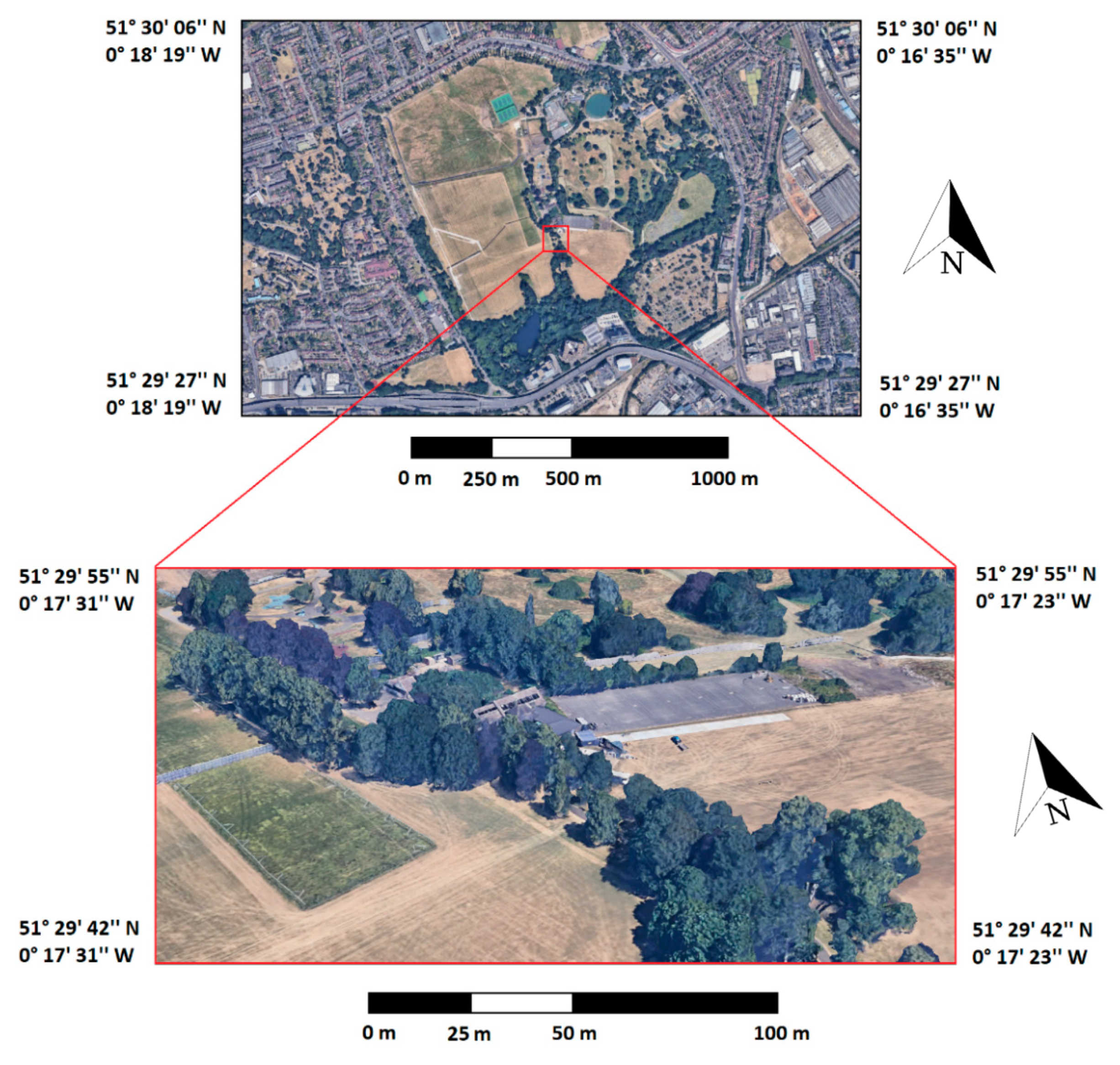
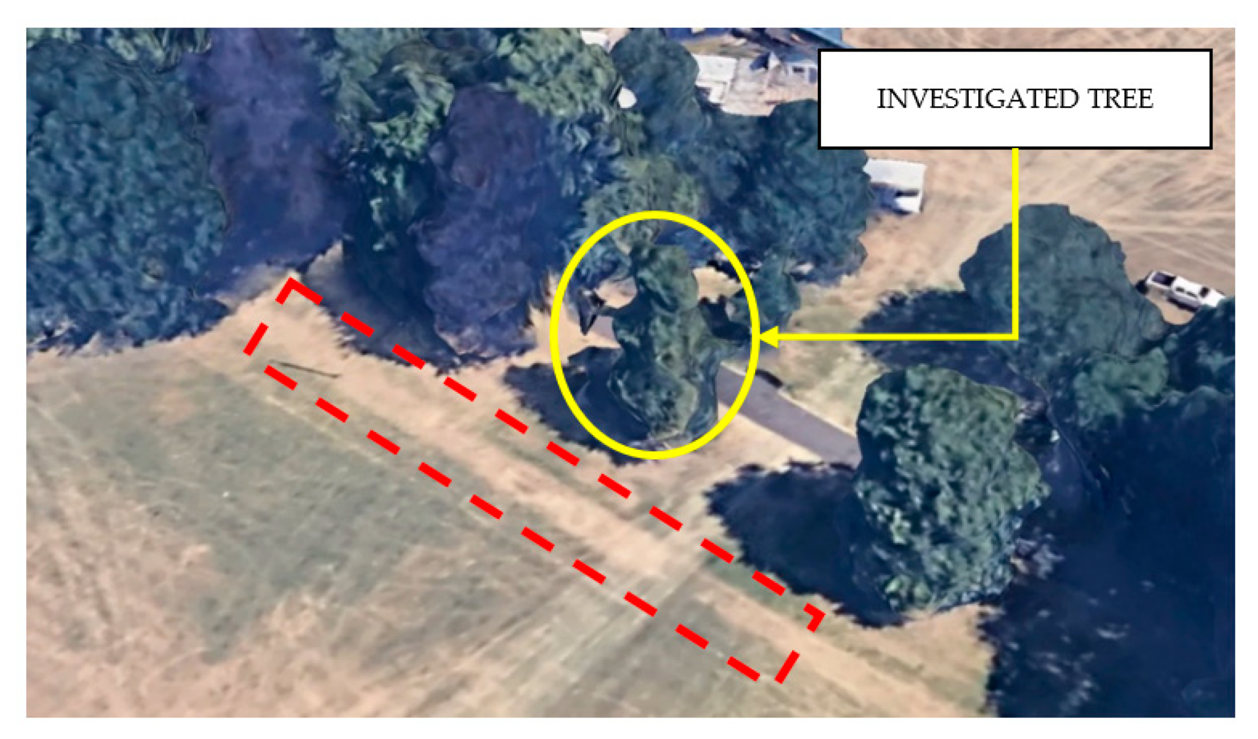
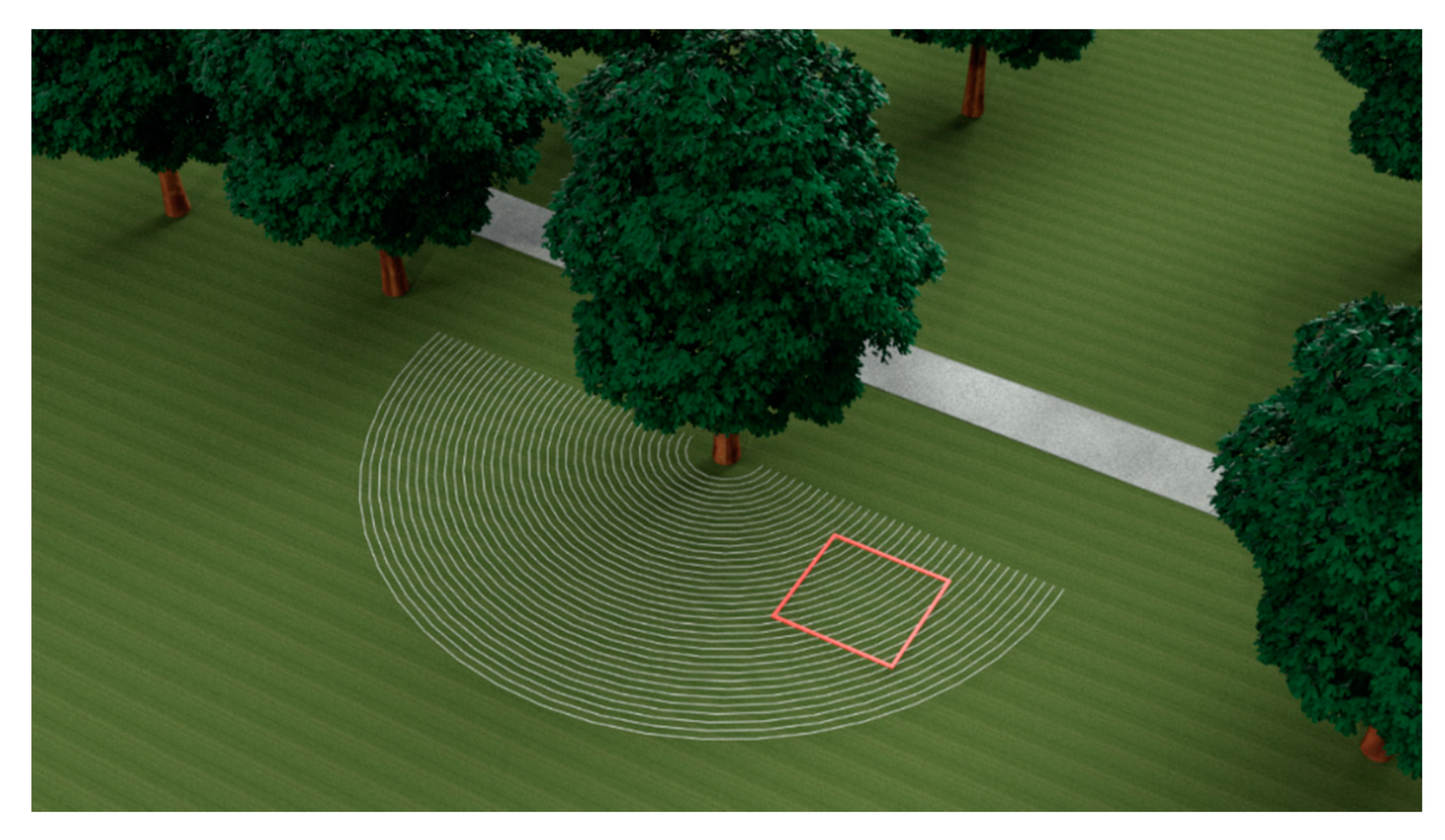
2.1. The Test Site

The survey was carried out in Gunnersbury Park, Ealing, London (United Kingdom) (Figure 1). The tree under investigation, a sycamore (Acer pseudoplatanus), was identified for this study by the London Borough of Ealing’s Tree Service. This tree is located along a tree-lined avenue inside the park, at a distance of ~10 m from the adjacent trees.

The concerned tree was under observation since 2010, according to the “Friends of Gunnersbury Park and Museum” registered charity, as “a significant cavity of over 10% of the stem was present” [40]. In the last decade, the tree’s conditions had deteriorated, as significant levels of rot and decay were found, creating hazards to local residents and users of the park. To this effect, a decision was made to cut the tree down and GPR investigations were carried out before falling the tree.

On the survey day, the weather was sunny, with temperatures between 19 and 21 °C and a humidity of 39%. Furthermore, it is important to note that the last episode of light rain occurred ten days before the survey [41].

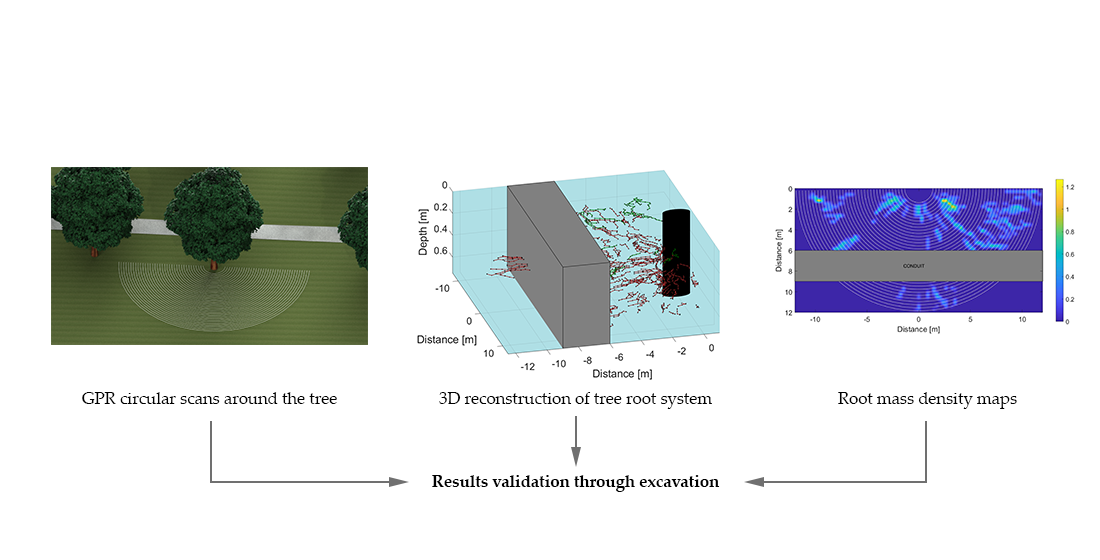
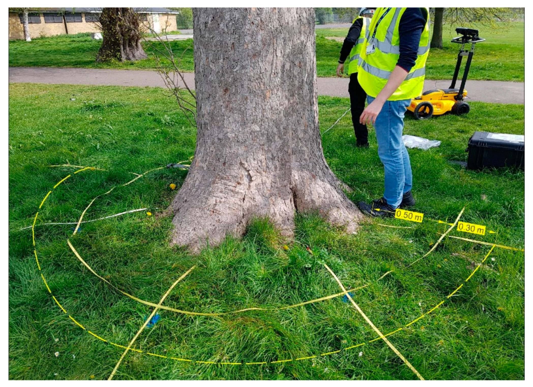
2.2. The GPR Survey Technique

The survey technique followed a circular GPR acquisition method, as described in [38]. This survey methodology was chosen due to the particular configuration of a typical root system, which expands radially from the trunk of the tree outwards [42,43]. In fact, GPR surveys carried out around the trunk with constant radial distance have proven capable of providing a quasi-perpendicular scan of the root systems [13].

Further, the investigation was carried out on the portion of the tree root system developing below the natural soil, excluding the area covered by an adjacent asphalt pavement (i.e., performing the scans along semi-circular transects) (Figure 2).

A set of 36 semi-circular scans were performed around the investigated tree. The first survey transect was positioned 0.50 m from the bark in order to allow enough space for the GPR equipment to manoeuvre around the tree trunk. Subsequently, the spacing between the lines of the scan was set to 0.30 m. Consequently, an overall area of 218.04 m² was surveyed around the tree, with an outer radius of 11.86 m and an inner radius of 1.36 m. Figure 3 shows a rendering of the GPR survey setup’s main characteristics.

2.3. The GPR Equipment

The Opera Duo ground-coupled GPR system, manufactured by IDS GeoRadar (part of Hexagon) was employed for testing purposes [13,44]. The system includes two mono-static antennas of 700 and 250 MHz central frequency. Data were collected using a time window of 80 ns, discretised across 512 samples. The horizontal resolution was set to 3.06 × 10⁻² m. For the purposes of this study, only data collected using the 700 MHz antenna were analysed in order to provide the highest effective resolution of the deepest layers of the root system.

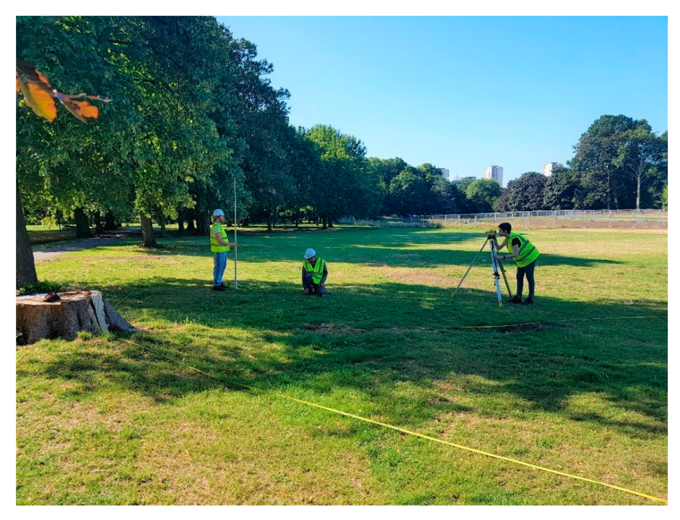
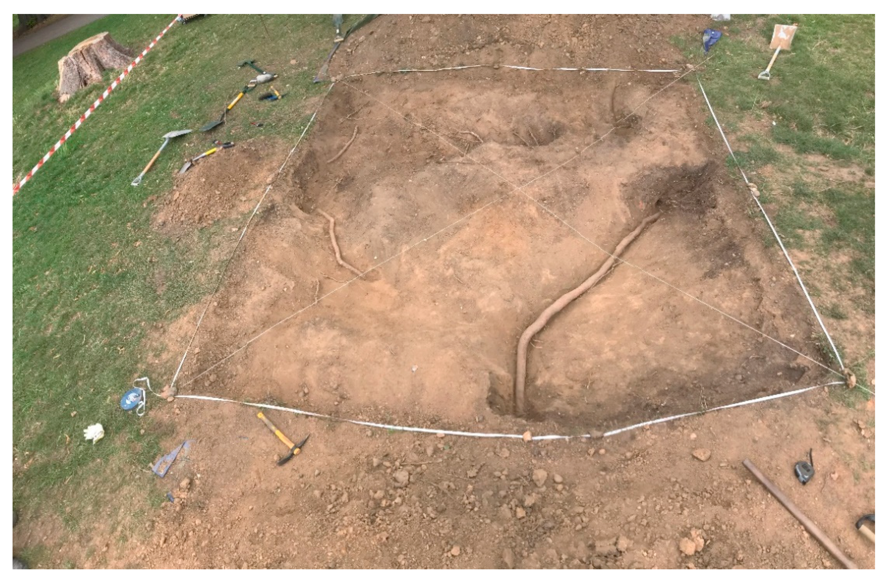
2.4. The Excavation for Validation Purposes

In order to validate the results obtained through the processing of the GPR data (described in detail in the following paragraphs), an excavation was carried out near the investigated tree. The exact location of the excavation area was determined a posteriori based on the results obtained in order to dig a defined area where the preliminary data analysis had highlighted the presence of potential targets.

The excavation took place approximately three months after the GPR survey. In the meantime, the tree was felled as planned, and it was necessary to wait for the technical time of the trunk removal from the investigation area. The whole activity, including finding the area coordinates, excavation, roots’ measurements and excavation coverage, was completed in three days.

An area of 4 m per side was accurately identified (Figure 4), based on the coordinates of the GPR survey (see Section 3.5). The excavation was then carried out by removing layers of ~0.10 m of soil at a time.

2.5. The Data Processing Framework

2.5.1. Preliminary Signal Processing Stage

The primary purpose of this stage is to reduce noise-related information from the GPR data, as well as to achieve quantitative information and easily interpretable images for the data analysis and interpretation stage. A signal processing methodology was implemented, based on a combination of standard and more advanced techniques [45,46], which can be applied to any GPR root system’s investigation. The raw data were therefore processed based on the following sequence of processing steps:

• Zero-offset removal: GPR signal can be distorted by a low-frequency signal trend (known as “wow”) or initial direct current (DC) shifts, which can conceal the actual EM reflections. The result is a GPR trace with an average amplitude different from zero, which could affect the results of further signal processing steps. The application of a dewow filter is used to obtain GPR traces with a mean value equal to zero.
• Time-zero correction: In order to compare the reflection time and consequently the depth of the buried targets, it is necessary to set a unique time-zero point for the GPR data. However, due to factors such as the air gap between the transmitting antenna and the soil surface or the ground-level inhomogeneities, the position of the air-ground surface reflection could vary across the different A-scans. To this extent, the air layer between the signal source point and the ground was eliminated across the whole sequence of A-scans.
• Time-varying gain: The GPR signal rapidly attenuates when it propagates through the investigated media. This is due to the dispersive nature of the EM waves, which relates to the electrical properties of the medium. For this reason, the response from deep targets can be barely detected, especially in case of lossy materials. The application of a time-varying gain to each GPR trace compensates for the rapid fall of the signal, equalising the amplitudes and making the response from deeper targets clearer. In the present study, a spherical and exponential (SEC) function was employed to compensate the energy loss by applying a linearly increasing time gain combined with an exponential increase.
• Singular value decomposition (SVD) [47]: The SVD filter aims to reduce the ringing noise, i.e., a repetitive type of clutter with a high correlation between traces, which can easily lead to data misinterpretation. On the other hand, reflections due to potential targets are more random and scattered, and therefore less correlated. The SVD filter operates by decomposing an image into a set of different sub-images, each of which contains features with a gradually increasing correlation. With this approach, ringing noise can be separated from the real response of the targets.
• Frequency-wavenumber (F-K) migration [47]: In a GPR investigation, the response of a target is associated with a hyperbolic feature. This is caused by the difference in the travel time of the EM waves, while the antenna is moved along the scanning transect. Although this output is acceptable for target identification, the tracking of an object (e.g., tree roots) across several B-scans requires a more focused and accurate localisation. The F-K migration transforms an unfocused space-time GPR image into a focused image showing the object’s true location and size with the corresponding EM reflectivity. The velocity of the host medium in this paper is assumed as constant and it was estimated by means of a trial and error procedure between permittivity values over-migrating and under-migrating the data.

2.5.2. Analysis of Discontinuity Elements

The presence of elements of discontinuity (e.g., manmade subsurface features such as pipes, conduits or the multi-layered structure of a road pavement) in a dataset including a tree root system architecture are regarded as a potential disruptive factor for the correct execution of the data processing methodologies presented in this paper.

In this specific case study, the presence of a transversal element in the investigated area, such as a road pavement and an underground pipe, interrupts the continuity of the data and creates the conditions for the generation of false alarms in the mapping process of the roots. The potential presence of these disturbing elements must therefore be identified before the application of the main tree root-tracking algorithm. For this purpose, a processing algorithm based on the methodology proposed in [48] is introduced in the main data processing framework. An analysis of the data reflectivity is carried out in order to identify the presence of features not related to roots clearly. If present, these inhomogeneities are subsequently reprocessed with dedicated signal processing techniques (e.g., in the case of a road pavement structures [48]), or their reflections are simply removed from the GPR data (e.g., in the case of pipes or other similar manmade buried features).

2.5.3. Tree Root-tracking Algorithm

This stage of the methodology is adapted from [38] and is composed of two main parts. First, the initial hypotheses (the data acquisition method and the dielectric properties of the medium), and the data input settings (the outcomes of the pre-processing algorithm, the matrix dimensions and the GPR data acquisition settings) were outlined.

Following this, an iterative procedure was executed in order to analyse the output of the pre-processing stage. The methodology was based on the comparison of the amplitude values, in a random position of the 3D domain, with a given threshold. The following steps were then performed:

• Preliminary hypotheses: The proposed model is based on two main hypotheses regarding:

  ∘

  The data acquisition method (longitudinal or circular transects), and

  ∘

  The dielectric properties of the investigated medium.

The acquisition method was performed by rotating the GPR antenna around the tree with a constant radial distance. As already stated, this was due to the radial distribution of roots around a tree trunk, and the necessity to achieve a quasi-perpendicular scan of the targets. The algorithm has therefore been developed with reference to a three-dimensional system of cylindrical coordinates, in which the vertical axis is identified by the axis of the tree trunk and the origin is positioned at its intersection with the plane matching the ground level. The coordinates of the system are the depth $z$, the angular coordinate $\theta$ and the radial coordinate $\rho$.

In regard to the relative dielectric permittivity of the medium ${\epsilon }_r$, this was calculated using a hyperbolic velocity analysis method. This compares the observed reflection hyperbolas with the velocity-specific hyperbolic functions in order to find the function that best fits the data [46]. For the purpose of this application, the wave propagation velocity v in the medium was taken as the average value of velocities, estimated by the application of the hyperbola fitting method to several roots’ reflections evenly picked up across the entire survey area.

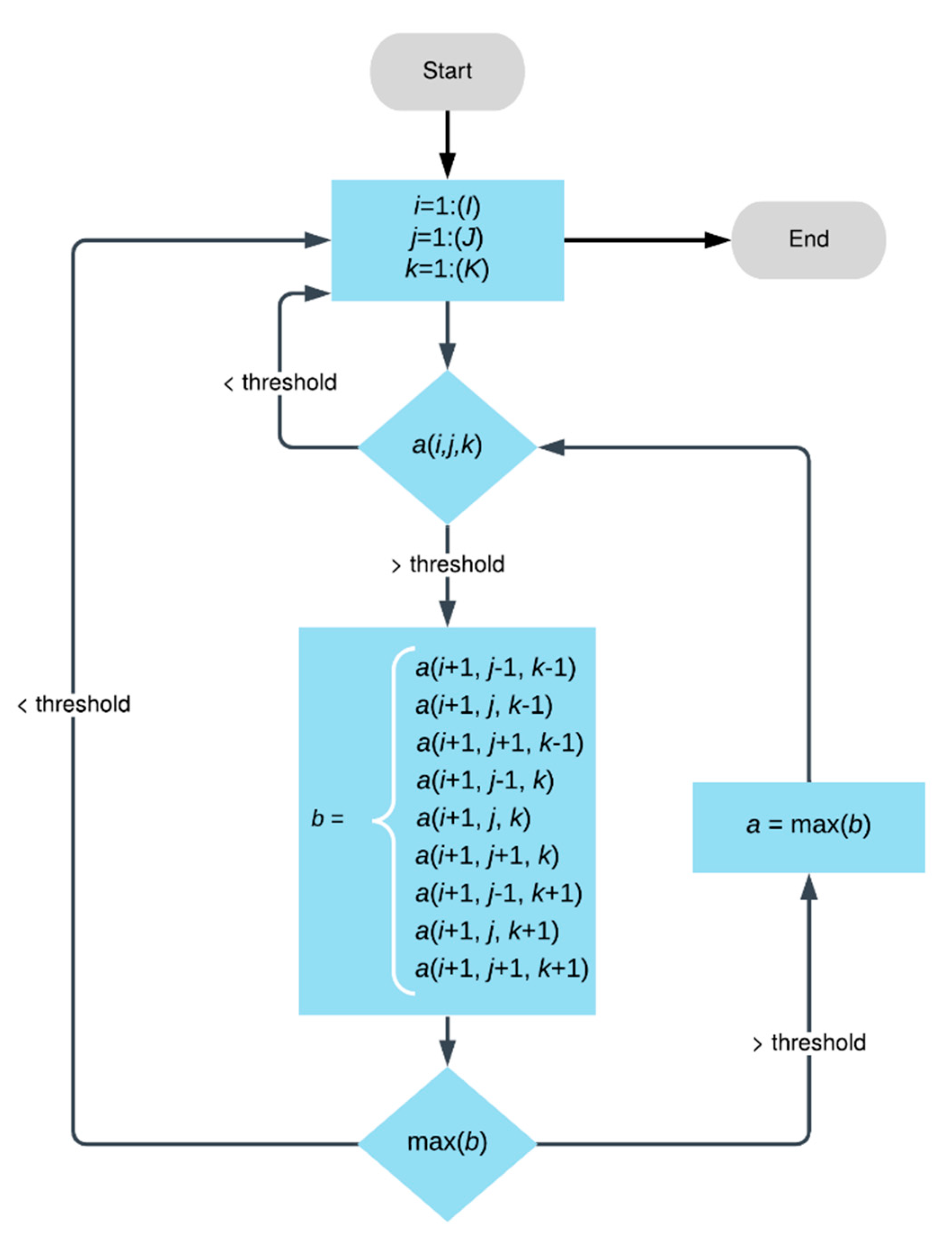
• Data input: The algorithm expands upon GPR data from the pre-processing phase, in the form of a three-dimensional matrix of real numbers $A\left(I,J,K\right)$, composed by the signal amplitude values in a random point of coordinates ($i,j,k$). The index $i$ indicates the number of GPR scans, limited to $I$, the index $j$ corresponds to the scan direction, limited to $J$, and $k$ is the vertical coordinate going into the ground, limited to $K$. According to a reference polar coordinate system, the coordinates of a random point $\left(i,j,k\right)$ can be expressed as follows:

  $$x=\rho \left(i\right)·cos\vartheta \left(j\right)$$

  (1)

  $$y=\rho \left(i\right)·sin\vartheta \left(j\right)$$

  (2)

  $$z=z\left(k\right)$$

  (3)
• Iterative procedure: The aforementioned assumptions and input information are essential to develop an iterative procedure for the tracking of a root system. Figure 5 shows a flowchart of the methodology followed in this stage.

  ∘

  Target identification: The algorithm evaluates the amplitude values in a random position of the 3D domain. In order to filter out the amplitude values that did not likely relate to tree roots, a threshold was set. This threshold value is established a priori based on a preliminary analysis of the data collected, in an effort to isolate as many hyperbolas as possible. Hence, the algorithm is set to analyse the domain until a signal amplitude value greater than the threshold is found. This step is necessary to identify the apices of the reflection hyperbolae (i.e., the apices of the roots) and filter out amplitude values unrelated to candidate root targets.

  ∘

  Correlation analysis: This step is focused on the investigation of further vertices in the closest vicinity of those identified at the target identification stage. This is performed to pinpoint other potential amplitude values greater than the threshold. This analysis has been improved in the present study compared to the original version presented in [38], as the area in which the correlation is sought has been extended to four further points within the 3D domain, i.e., a(i + 1, j − 1, k − 1), a(i + 1, j + 1, k − 1), a(i + 1, j − 1, k + 1), a(i + 1, j + 1, k + 1) (see Figure 5). This improvement is used to smooth the correlation analysis process, including all the points of the 3D domain that could ideally belong to the development of a root.

  ∘

  Tracking of the root: The algorithm isolates correlated points, creating a vector for the mapping of individual roots.

  ∘

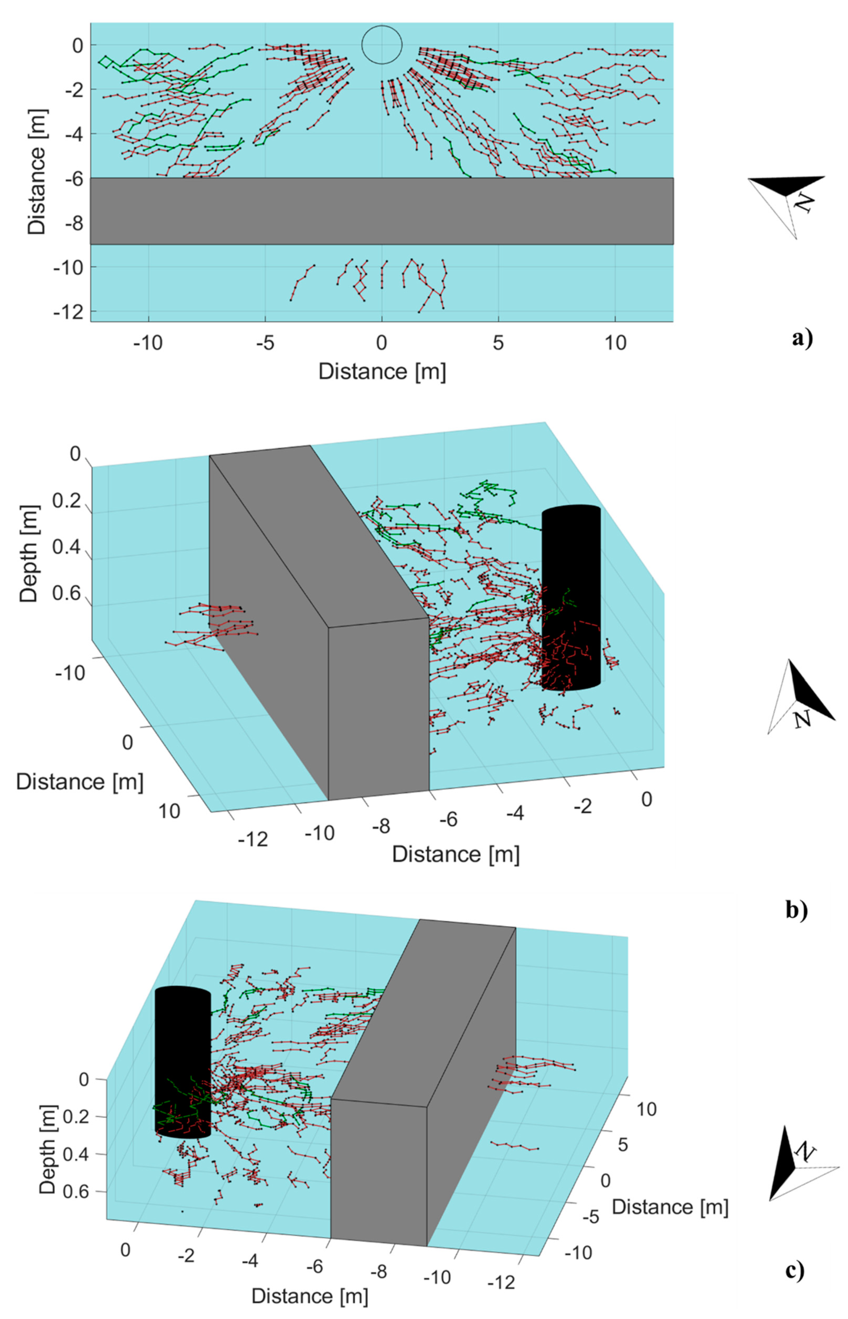
  Reconstruction of the root system architecture in a 3D domain: Vectors identified in the previous step are positioned in a 3D environment in order to represent the geometry of the tree root system.

It is important to point out that in order to avoid the inclusion in the map of roots not belonging to the investigated tree, the root mapping algorithm is designed to perform a spatial correlation that follows the most likely directions of roots (i.e., from the trunk—source point—outwards). Therefore, the resulting renderings are only related to the examined tree, and do not include any potential root belonging to adjacent trees (Figure 6). If present, these will result as uncorrelated with the mapping process and, hence, will be excluded by the algorithm.

2.5.4. Root Mass Density Estimation

At present, the quantification of the tree roots mass density is considered a controversial task. In this regard, it should be specified that most of the studies deal with the quantification of tree root’s biomass, which is an indirect output of GPR data [19]. Several studies have been carried out on this topic, both in field conditions [37] and in a controlled environment [49], achieving reasonably good results. However, the accuracy of current methodologies still is limited. At present, the limiting factor for a correct root density estimate is the root water content that, if too low, can lead to a sub-estimation of root biomass. It should be concluded that existing evaluation methods are currently unable to provide reliable estimates. In this context, the novelty of the presented methodology lies in a new root density index evaluation, based on root location and length as obtained from the root mapping algorithm modelling process. The following stage of the presented methodology is therefore developed to provide a representation of the density of roots in the investigated area, with the main aim of identifying local changes of density.

First, best-fitting functions were used to better approximate root paths in the 3D domain, as well as to identify the length of each root in a continuous domain. Before evaluating the length of the roots in a specified domain, it is necessary to express these in an analytical form. Each root is a 3D curve with a radial expansion that starts from the centre of the tree trunk. The only way to express 3D curves is through parametric equations or positional vectors [50]. As an example, a 3D curve can be expressed either as:

$$x=f\left(t\right)$$

(4)

$$y=g\left(t\right)$$

(5)

$$z=q\left(t\right)$$

(6)

or as:

$$\overrightarrow{F}=f\left(t\right),g\left(t\right),q\left(t\right)$$

(7)

where $\{t\in R|0\le t\le 1$} is the parametric variable between zero and one that is chosen arbitrarily. To fit a parametric curve on a given set of 3D points, a polynomial function of nth order is used to approximate each of the parametric functions [50]

$$x={\displaystyle \sum }_{i=0}^n{a}_i{t}^i$$

(8)

$$y={\displaystyle \sum }_{i=0}^n{b}_i{t}^i$$

(9)

$$z={\displaystyle \sum }_{i=0}^n{c}_i{t}^i$$

(10)

The coefficients $a_i,b_i,c_i$ are evaluated using least squares [51]:

$$\mathit{A}=(W^T{W)}^{-1}{W}^T\mathit{X}$$

(11)

$$\mathit{B}={(W^{T}W)}^{-1}{W}^T\mathit{Y}$$

(12)

$$\mathit{C}={(W^{T}W)}^{-1}{W}^T\mathit{Z}$$

(13)

where A, B and C are vectors $\left\{\mathrm{A},\mathrm{B},\mathrm{C}\in R^n\right\}$ that contain the coefficients $a_i,b_i,c_i$. The matrices X, Y and Z are column vectors $\left\{\mathit{X},\mathit{Y},\mathit{Z}\in R^s\right\}$ that contain the predicted $x, y, z$ coordinates using the root-detection algorithm. The number of measurements is denoted with the letter s. Notably, when $n>s$, the system becomes underdetermined and no solution without constraints can be obtained. Thus, the number of measurements must always be greater than or equal to the order of the chosen polynomial. Lastly the matrix W $\{W\in R^{n\times s}$} is:

$$\mathit{W}=\left[\begin{array}{ccc}{t}_1^n& \cdots & t_1^0\\ ⋮& \ddots & ⋮\\ t_s^n& \cdots & t_s^0\end{array}\right]$$

(14)

where $t_1,t_2\dots .t_s$, $\{t\in R|t_{i+1}-t_i=\frac{1}{s}\}$ are a set of equidistant points defined in the closed interval [0,1].

Knowing the analytical expression of the vector $\overrightarrow{F}$ makes it possible to evaluate its length for a given sample. The length of vector $\overrightarrow{F}$ with respect to $t$ equals with [50]:

$$L\left(t\right)={{\displaystyle \int }}_0^t\frac{d\overrightarrow{F}}{dt}dt$$

(15)

The derivative of the vector $\overrightarrow{F}$ with respect to $t$, equals with the derivative of its components:

$$\frac{dx}{dt}={\displaystyle \sum }_{i=1}^{n}i{a}_i{t}^{i-1}$$

(16)

$$\frac{dy}{dt}={\displaystyle \sum }_{i=1}^{n}i{b}_i{t}^{i-1}$$

(17)

$$\frac{dz}{dt}={\displaystyle \sum }_{i=1}^{n}i{c}_i{t}^{i-1}$$

(18)

Therefore, the integral in (15) can be rewritten as [50]:

$$L\left(t\right)={{\displaystyle \int }}_0^t\sqrt{{\left({\displaystyle \sum }_{i=1}^{n}i{a}_i{t}^{i-1}\right)}^2+{\left({\displaystyle \sum }_{i=1}^{n}i{b}_i{t}^{i-1}\right)}^2+{\left({\displaystyle \sum }_{i=1}^{n}i{c}_i{t}^{i-1}\right)}^2}dt$$

(19)

The integral above is evaluated using numerical methods (Simpson’s rule, Gaussian quadrature) [52]. The length $L$ is related to $t$, thus it can be calculated for a given segment, giving us the ability to map the length of the roots in a specified domain. The degree of the polynomial $n$ should be chosen with caution since large values can give rise to over-fitting, resulting in poor generalisation capabilities of the fitted polynomial, whereas small values can decrease the overall resolution. As a rule of thumb, the order of the polynomial should be less than half the number of measurements $n<s/2$.

Once the length of the root was known, the domain was partitioned into reference volume units, the dimensions of which depend on the circular scan spacing and the depth resolution required for the density investigation. The length of roots contained in the reference volume was then evaluated as follows:

$$d=\frac{{{\displaystyle \sum }}_{i=1}^n{L}_i}{V}$$

(20)

where $d$ is the density [m/m³], $n$ is the number of roots contained in a reference unit of volume $V$ [m³] and $L_i$ is the length of the root [m].

3. Results

3.1. Preliminary Signal Processing Stage

The use of a pre-processing phase on the GPR data enabled achieving a more effective detection of targets with a significant reduction in noise-related features. To elaborate, the application of the SVD filter reduced the effect of reflections from the horizontal layers as well as the multiple reflection patterns caused by ringing noise. Figure 7 shows the result of the application of the discussed signal processing steps. Figure 7a,b clearly show the application of the standard processing techniques and the SVD filter. In particular, the latter has proven effective in significantly removing noise-related features.

Moreover, the application of the F–K migration filter enabled obtaining a more focused representation of the hyperbolic targets, including the roots, hence contributing to improvethe effectiveness of the proposed algorithm in the next phase. It is in fact fair to comment that, without the application of this particular filter, false alarms were frequent, i.e., points belonging to the tail of the hyperbolas (therefore not representing the actual position of the target) with amplitude values satisfying the threshold value conditions. These points were not discarded by the algorithm and generated false positives. Thus, the application of the migration process has proven to increase the reliability of the algorithm for the detection and tracking of roots in the subsequent steps. Figure 7c shows the result of the F-K migration to the pre-processed data. It is possible to notice how the tails of the hyperbolas have retracted towards the apexes (i.e., the real position of the targets), forming unique focused points. In addition, it is important to observe that the migration provided an estimation for the value of the permittivity equal to 12, which corresponds to a velocity of the electromagnetic wave equal to 4.33 × 10⁷ m/s.

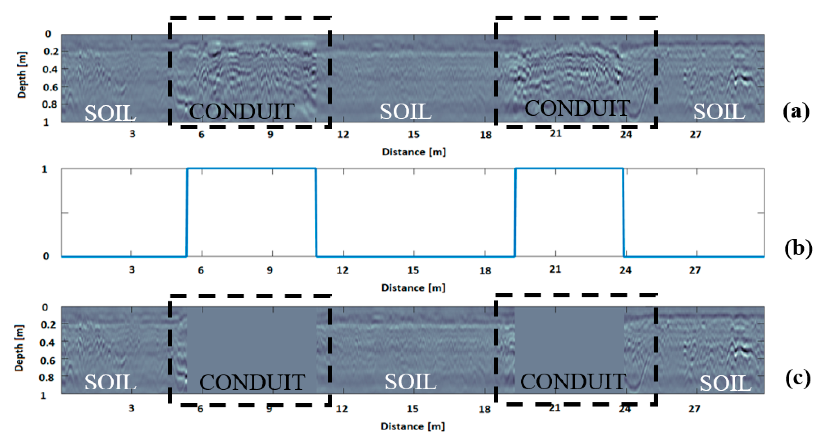
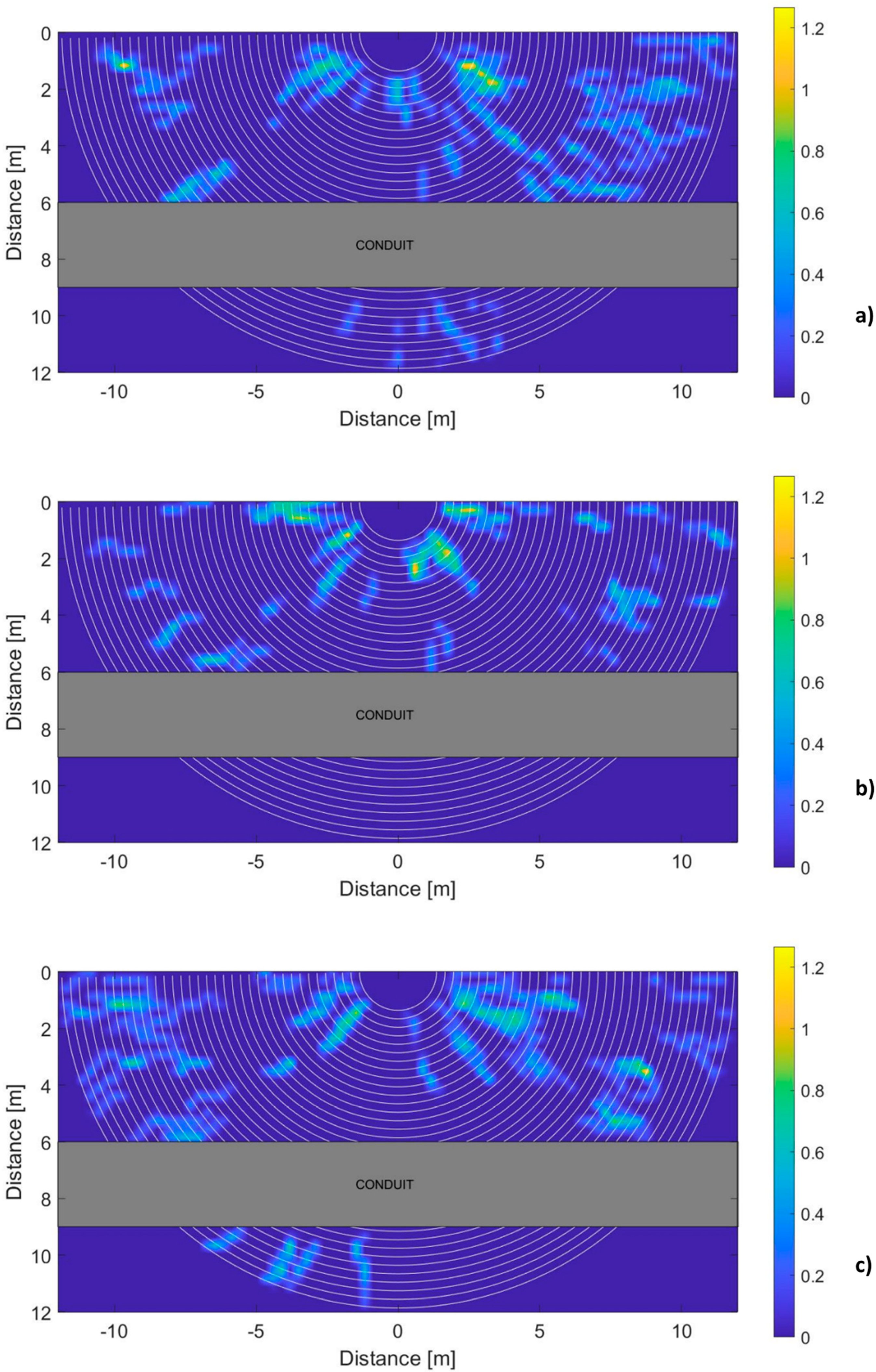
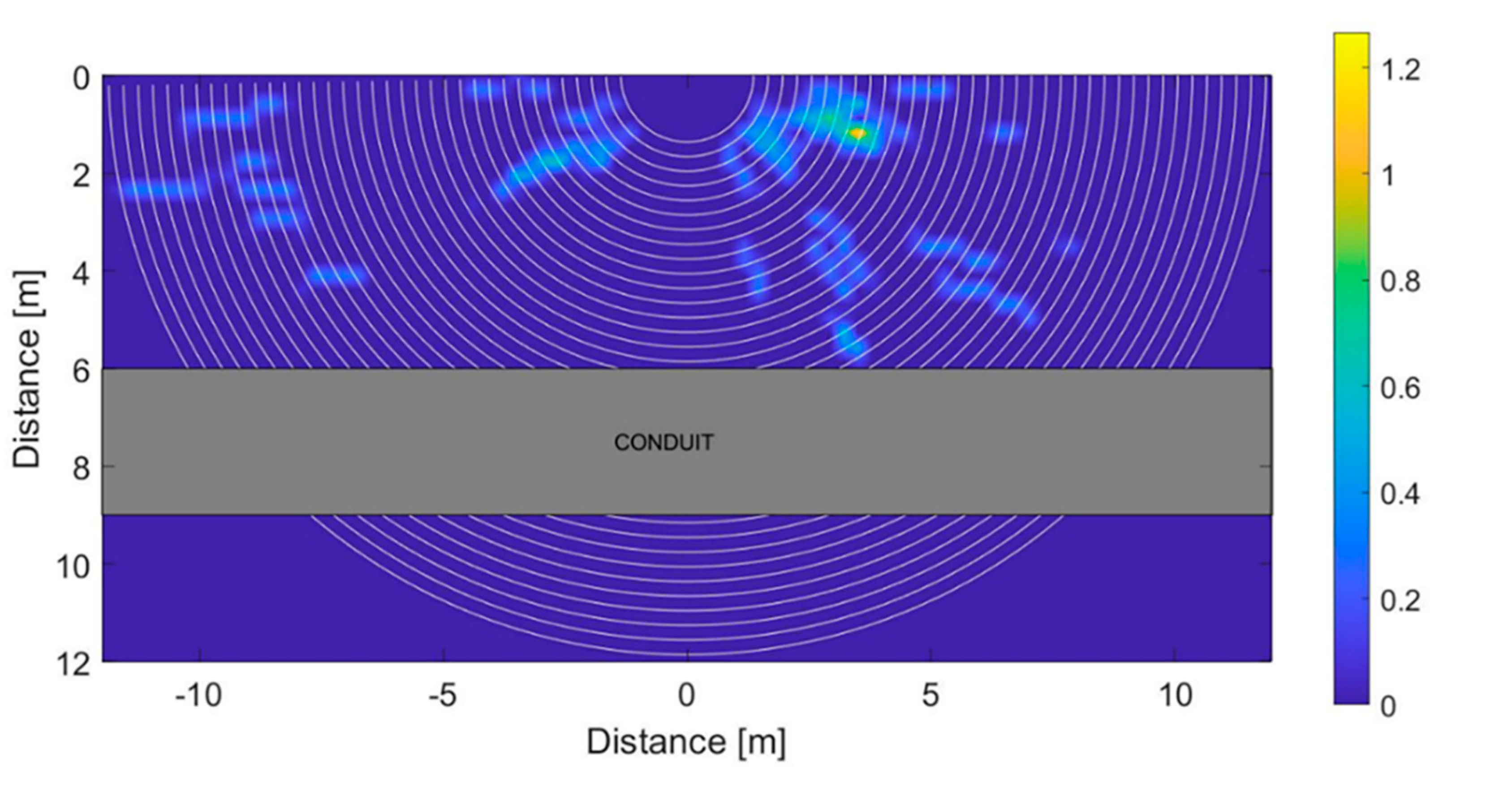
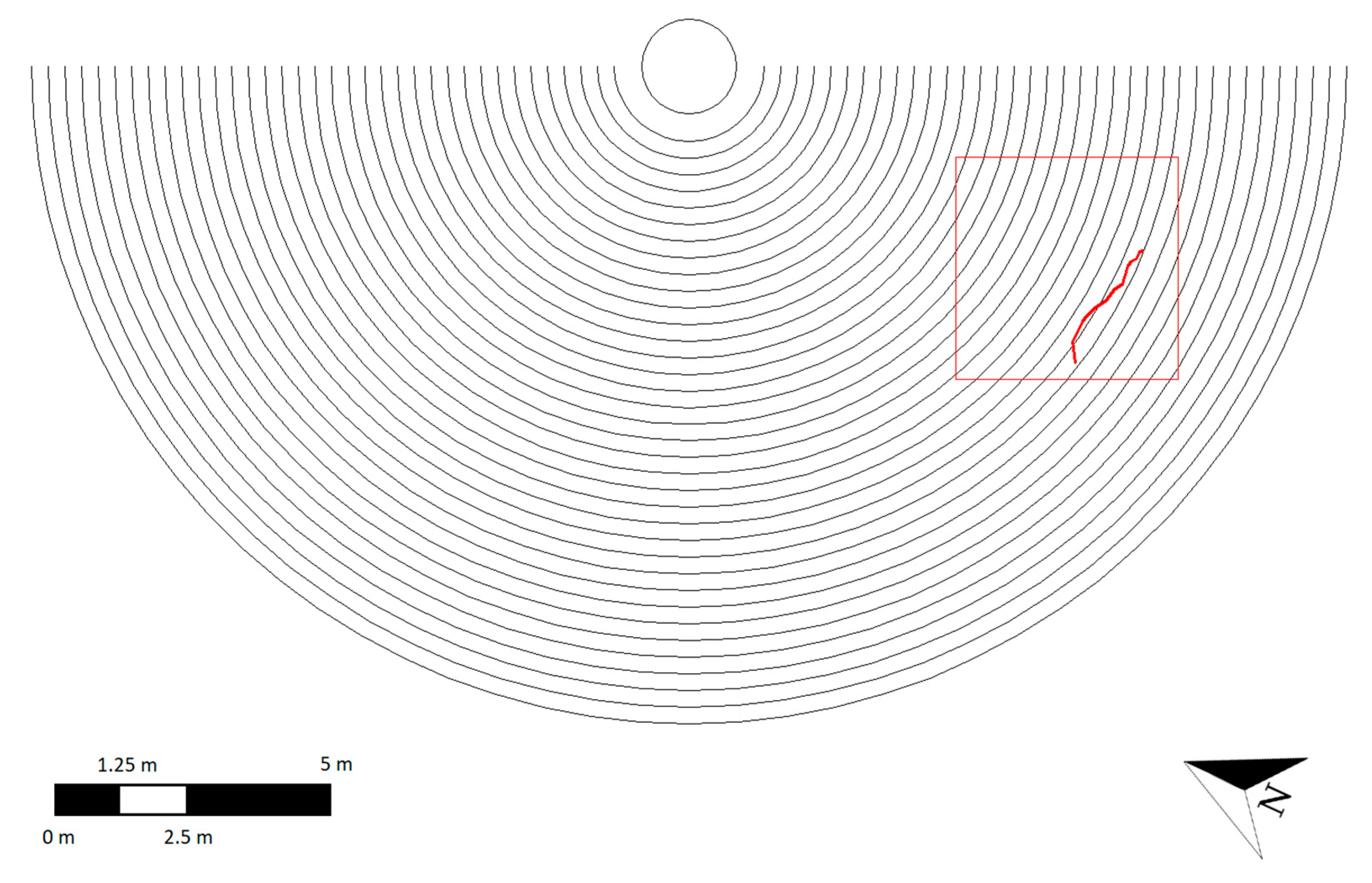
3.2. Analysis of Discontinuity Elements: the Detection of a Buried Structure

An in-depth analysis of potential elements of discontinuity across the collected set of B-scans—as per the requirements discussed in Section 2.5.2—revealed the presence of a buried structure, recurring from scan 17 onwards (Figure 8). In order to better understand the nature of such a feature, a tomographic approach was followed to allow for a more comprehensive analysis of the investigated area. For this purposes, C-scans [45] were created at different depths, which highlighted the presence of a subsurface linear structure, approximately 2 m wide and 5 m distant from the tree, crossing the investigation area (Figure 9). The analysis of both B-scans and C-scans suggests the presence of a reinforced concrete structure, as hyperbolic and evenly spaced reflections, potentially attributable to reinforcement bars, can be observed. Considering the layout of the site and the characteristics of the feature (i.e., estimated dimensions and construction materials), the latter was interpreted to be a conduit, serving an artificial lake located in the vicinity of the survey area.

In addition to the above, it is important to note that a difference in the appearance of the ground was noticed, based on a visual inspection carried out on the study area. This feature was observed exactly at the location coordinates of the identified structure (Figure 10). It is therefore reasonable to assume that a conduit was introduced in relatively recent times, and that the required excavation and groundwork have interfered with the existing root system, cutting off roots and undermining the already decayed conditions of the tree.

In terms of the data processing, the presence of this particular feature interferes with the application of the tree root-tracking algorithm in the following stages. In addition, it implies that no roots are present within the volume occupied by the identified underground structure. For the purposes of this study, it was therefore decided to remove the reflections related to this particular type of discontinuity feature. A processing framework based on the methodology introduced in [48] was hence followed. The analysis of the data reflectivity was carried out to quantitatively locate the buried structure and eliminate the related reflections from the B-scans. Figure 11 shows the application of this processing scheme, proving that analysing the signal reflectivity is a valid tool to achieve an accurate detection of major elements of discontinuity.

3.3. Tree Root-Tracking Algorithm

Following the application of the preliminary signal processing stage and the analysis of the signal discontinuity, the tree root-tracking algorithm was applied for the reconstruction of the root system architecture in a three-dimensional environment. Figure 12 shows the outcome of this procedure, which is a 2D planar view (a) and a 3D view (b and c) of the reconstructed root system architecture. To aid with the interpretation of results, shallow-buried roots (i.e., within the first 25 cm of soil) and deeper roots (i.e., below the first 25 cm of soil) have been represented with different colours.

The analysis of the results showed that reflections were located within the first 0.70 m of soil. This is apparently not in line with the expectation for the root system of sycamore trees, as their roots can reach a depth of approximately 1.40–1.50 m [53,54]. Nevertheless, Crow [54] reports that 90% to 99% of tree roots are usually found within the first metre of soil. The absence of reflections from deeper roots could be linked to the presence of death roots, having a value of dielectric permittivity close to that of the soil. Similarly, as shown in Figure 12, a discontinuity of the root system is visible in certain areas, mainly in the central region of the investigated soil. This could likely be an effect of the conduit installation, which may have interfered with the original structure of the root system and caused irreversible damage.

Finally, it is worth noting that the algorithm is designed to discard shorter segments, which might relate to non-root targets (e.g., boulders). The results achieved at this stage of the data processing are consistent with this particular algorithm feature.

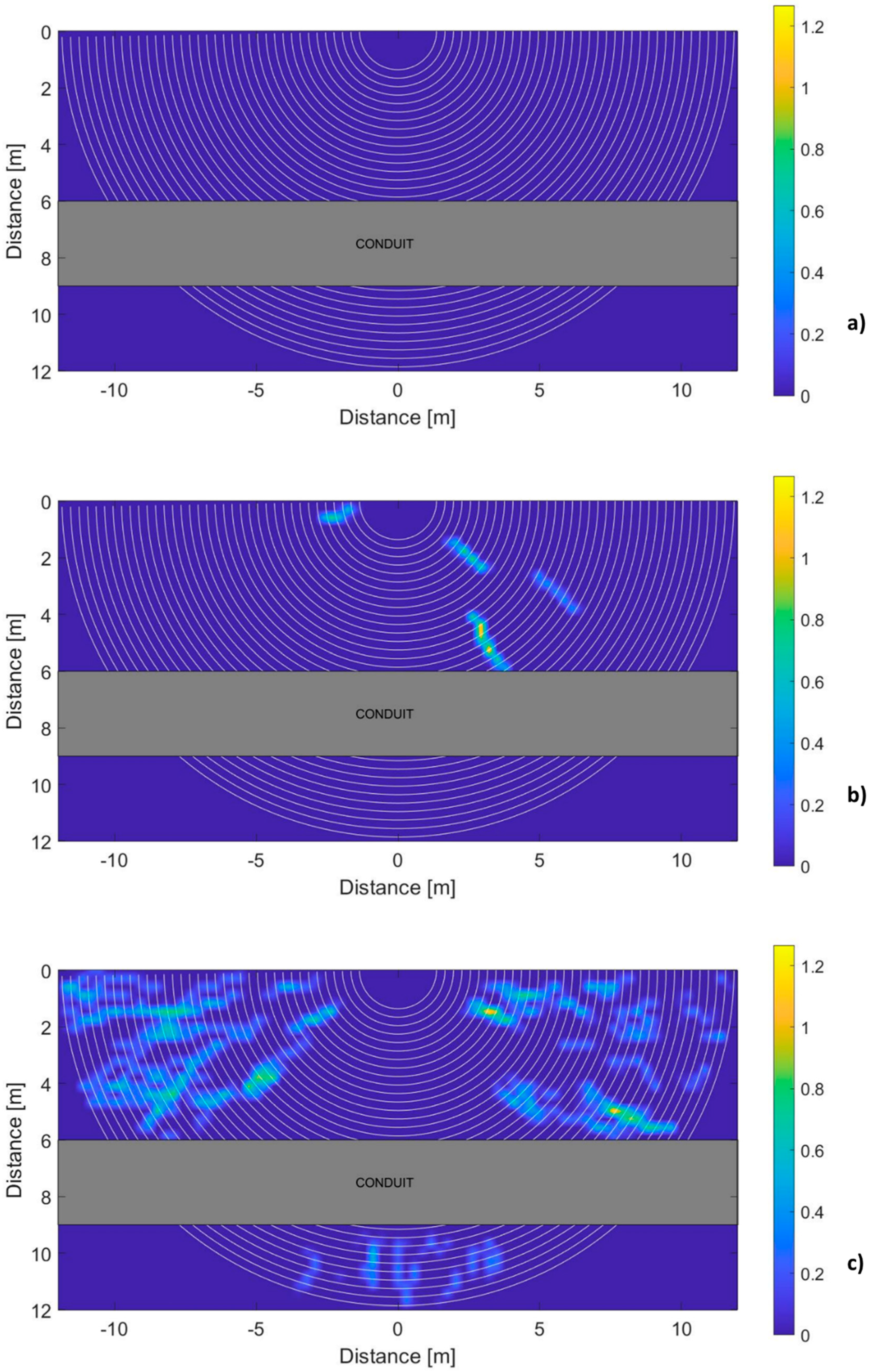
3.4. The Root Mass Density Maps

The architecture of the root system was then further investigated through the evaluation of the root density at different depths (Equation (20)). The investigated domain was divided into reference volumes of 0.30 m × 0.30 m × 0.10 m, where the dimension 0.30 m was chosen for consistency with the spacing between the scans, and the depth dimension 0.10 m was selected for consistency with the excavation steps performed at the validation stage. Hence, the domain was analysed to determine the total root length per reference unit.

Figure 13, Figure 14 and Figure 15 show the outcomes of this processing stage, where several areas with a high density of roots can be identified. In order to further analyse the density variations, the maps were divided into homogeneous zones, as shown in

Table 1. Root mass density zoning for the investigated tree.

Root Mass Density Zoning
Depth [m]	x		y		Minimum Value [m/m3]	Maximum Value [m/m3]	Average Value [m/m3]	Standard Deviation [m/m3]
	From [m]	To [m]	From [m]	To [m]
0.10–0.20	−12.60	−8.40	0.00	4.20	0.00	0.00	0.00	0.00
	−8.40	−4.20	0.00	4.20	0.00	0.00	0.00	0.00
	−4.20	0.00	0.00	4.20	0.00	0.67	0.01	0.08
	0.00	4.20	0.00	4.20	0.00	0.76	0.02	0.10
	4.20	8.40	0.00	4.20	0.00	0.35	0.01	0.05
	8.40	12.60	0.00	4.20	0.00	0.00	0.00	0.00
	−12.60	−8.40	4.20	8.40	0.00	0.00	0.00	0.00
	−8.40	−4.20	4.20	8.40	0.00	0.00	0.00	0.00
	−4.20	0.00	4.20	8.40	0.00	0.00	0.00	0.00
	0.00	4.20	4.20	8.40	0.00	1.05	0.03	0.15
	4.20	8.40	4.20	8.40	0.00	0.00	0.00	0.00
	8.40	12.60	4.20	8.40	0.00	0.00	0.00	0.00
	−12.60	−8.40	8.40	12.60	0.00	0.00	0.00	0.00
	−8.40	−4.20	8.40	12.60	0.00	0.00	0.00	0.00
	−4.20	0.00	8.40	12.60	0.00	0.00	0.00	0.00
	0.00	4.20	8.40	12.60	0.00	0.00	0.00	0.00
	4.20	8.40	8.40	12.60	0.00	0.00	0.00	0.00
	8.40	12.60	8.40	12.60	0.00	0.00	0.00	0.00
0.20–0.30	−12.60	−8.40	0.00	4.20	0.00	0.91	0.15	0.21
	−8.40	−4.20	0.00	4.20	0.00	1.05	0.15	0.23
	−4.20	0.00	0.00	4.20	0.00	0.88	0.04	0.13
	0.00	4.20	0.00	4.20	0.00	1.44	0.06	0.19
	4.20	8.40	0.00	4.20	0.00	0.91	0.09	0.18
	8.40	12.60	0.00	4.20	0.00	0.58	0.05	0.12
	−12.60	−8.40	4.20	8.40	0.00	0.91	0.07	0.17
	−8.40	−4.20	4.20	8.40	0.00	1.07	0.06	0.17
	−4.20	0.00	4.20	8.40	0.00	0.00	0.00	0.00
	0.00	4.20	4.20	8.40	0.00	0.75	0.01	0.07
	4.20	8.40	4.20	8.40	0.00	1.41	0.10	0.21
	8.40	12.60	4.20	8.40	0.00	0.92	0.03	0.14
	−12.60	−8.40	8.40	12.60	0.00	0.00	0.00	0.00
	−8.40	−4.20	8.40	12.60	0.00	0.00	0.00	0.00
	−4.20	0.00	8.40	12.60	0.00	0.65	0.04	0.10
	0.00	4.20	8.40	12.60	0.00	0.36	0.04	0.09
	4.20	8.40	8.40	12.60	0.00	0.00	0.00	0.00
	8.40	12.60	8.40	12.60	0.00	0.00	0.00	0.00
0.30–0.40	−12.60	−8.40	0.00	4.20	0.00	1.27	0.05	0.15
	−8.40	−4.20	0.00	4.20	0.00	0.57	0.03	0.09
	−4.20	0.00	0.00	4.20	0.00	0.86	0.10	0.20
	0.00	4.20	0.00	4.20	0.00	1.27	0.14	0.24
	4.20	8.40	0.00	4.20	0.00	0.68	0.06	0.13
	8.40	12.60	0.00	4.20	0.00	0.73	0.10	0.17
	−12.60	−8.40	4.20	8.40	0.00	0.43	0.00	0.03
	−8.40	−4.20	4.20	8.40	0.00	0.74	0.04	0.13
	−4.20	0.00	4.20	8.40	0.00	0.00	0.00	0.00
	0.00	4.20	4.20	8.40	0.00	0.55	0.02	0.08
	4.20	8.40	4.20	8.40	0.00	0.76	0.08	0.17
	8.40	12.60	4.20	8.40	0.00	0.31	0.01	0.05
	−12.60	−8.40	8.40	12.60	0.00	0.00	0.00	0.00
	−8.40	−4.20	8.40	12.60	0.00	0.00	0.00	0.00
	−4.20	0.00	8.40	12.60	0.00	0.34	0.01	0.05
	0.00	4.20	8.40	12.60	0.00	0.50	0.03	0.09
	4.20	8.40	8.40	12.60	0.00	0.00	0.00	0.00
	8.40	12.60	8.40	12.60	0.00	0.00	0.00	0.00
0.40–0.50	−12.60	−8.40	0.00	4.20	0.00	0.35	0.02	0.07
	−8.40	−4.20	0.00	4.20	0.00	0.63	0.04	0.12
	−4.20	0.00	0.00	4.20	0.00	1.09	0.10	0.21
	0.00	4.20	0.00	4.20	0.00	1.06	0.12	0.23
	4.20	8.40	0.00	4.20	0.00	0.67	0.04	0.12
	8.40	12.60	0.00	4.20	0.00	0.65	0.04	0.12
	−12.60	−8.40	4.20	8.40	0.00	0.49	0.01	0.05
	−8.40	−4.20	4.20	8.40	0.00	0.62	0.03	0.11
	−4.20	0.00	4.20	8.40	0.00	0.00	0.00	0.00
	0.00	4.20	4.20	8.40	0.00	0.31	0.01	0.06
	4.20	8.40	4.20	8.40	0.00	0.39	0.01	0.05
	8.40	12.60	4.20	8.40	0.00	0.32	0.00	0.03
	−12.60	−8.40	8.40	12.60	0.00	0.00	0.00	0.00
	−8.40	−4.20	8.40	12.60	0.00	0.00	0.00	0.00
	−4.20	0.00	8.40	12.60	0.00	0.00	0.00	0.00
	0.00	4.20	8.40	12.60	0.00	0.00	0.00	0.00
	4.20	8.40	8.40	12.60	0.00	0.00	0.00	0.00
	8.40	12.60	8.40	12.60	0.00	0.00	0.00	0.00
0.50–0.60	−12.60	−8.40	0.00	4.20	0.00	1.01	0.12	0.19
	−8.40	−4.20	0.00	4.20	0.00	0.62	0.05	0.13
	−4.20	0.00	0.00	4.20	0.00	1.11	0.10	0.22
	0.00	4.20	0.00	4.20	0.00	1.02	0.16	0.24
	4.20	8.40	0.00	4.20	0.00	1.00	0.10	0.19
	8.40	12.60	0.00	4.20	0.00	1.41	0.07	0.17
	−12.60	−8.40	4.20	8.40	0.00	0.45	0.02	0.08
	−8.40	−4.20	4.20	8.40	0.00	0.60	0.04	0.11
	−4.20	0.00	4.20	8.40	0.00	0.00	0.00	0.00
	0.00	4.20	4.20	8.40	0.00	0.29	0.00	0.03
	4.20	8.40	4.20	8.40	0.00	1.00	0.05	0.14
	8.40	12.60	4.20	8.40	0.00	0.64	0.01	0.07
	−12.60	−8.40	8.40	12.60	0.00	0.00	0.00	0.00
	−8.40	−4.20	8.40	12.60	0.00	0.81	0.03	0.12
	−4.20	0.00	8.40	12.60	0.00	0.86	0.05	0.15
	0.00	4.20	8.40	12.60	0.00	0.00	0.00	0.00
	4.20	8.40	8.40	12.60	0.00	0.00	0.00	0.00
	8.40	12.60	8.40	12.60	0.00	0.00	0.00	0.00
0.60–0.70	−12.60	−8.40	0.00	4.20	0.00	0.34	0.04	0.09
	−8.40	−4.20	0.00	4.20	0.00	0.30	0.00	0.03
	−4.20	0.00	0.00	4.20	0.00	0.66	0.04	0.11
	0.00	4.20	0.00	4.20	0.00	1.24	0.10	0.18
	4.20	8.40	0.00	4.20	0.00	0.36	0.02	0.08
	8.40	12.60	0.00	4.20	0.00	0.00	0.00	0.00
	−12.60	−8.40	4.20	8.40	0.00	0.00	0.00	0.00
	−8.40	−4.20	4.20	8.40	0.00	0.35	0.01	0.04
	−4.20	0.00	4.20	8.40	0.00	0.00	0.00	0.00
	0.00	4.20	4.20	8.40	0.00	0.56	0.02	0.08
	4.20	8.40	4.20	8.40	0.00	0.33	0.01	0.06
	8.40	12.60	4.20	8.40	0.00	0.00	0.00	0.00
	−12.60	−8.40	8.40	12.60	0.00	0.00	0.00	0.00
	−8.40	−4.20	8.40	12.60	0.00	0.00	0.00	0.00
	−4.20	0.00	8.40	12.60	0.00	0.00	0.00	0.00
	0.00	4.20	8.40	12.60	0.00	0.00	0.00	0.00
	4.20	8.40	8.40	12.60	0.00	0.00	0.00	0.00
	8.40	12.60	8.40	12.60	0.00	0.00	0.00	0.00

. The minimum and maximum density values, the average density and standard deviation were calculated at every identified area.

From the analysis of the density maps, the domain portion with a greater root mass density is from a depth of 0.20 m to a depth of 0.60 m (Figure 13c and Figure 14). This is also supported by the analysis of the maximum values reported in Table 1 for these depths. More specifically, the left quadrant of the investigated domain presents a greater density of roots between 0.20 m and 0.30 m of depth, with maximum values ranging from 0.88 m/m³ to 1.05 m/m³ (Table 1 −x coordinates −12.60 m to 0.00 m, y coordinates 0.00 m to 4.20 m) (Figure 13c), and between 0.50 m and 0.60 m of depth, with maximum values between 1.00 m/m³ and 1.11 m/m³ (Table 1 −x coordinates −12.60 m to 0.00 m, y coordinates 0.00 m to 4.20 m) (Figure 14c). On the other hand, the right quadrant presents higher values of root density between 0.20 m and 0.40 m, with peaks up to 1.44 m/m³ (Table 1 −x coordinates 0.00 m to 4.20 m, y coordinates 0.00 m to 4.20 m, depth 0.20–0.30 m) (Figure 13c and Figure 14a). A higher root density on the left and the right quadrants can be interpreted as an indirect consequence of the root system’s interconnection with two adjacent trees, located respectively on the North-West and the South-East directions from the investigated one. In fact, it is reasonable to assume that the root density of a specific tree could be higher at root interconnection areas, as roots of individual trees tend to have a closer arrangement between themselves, due to their own interaction with the root systems of adjacent trees. Finally, it should be emphasised that, although the aforementioned high root density concentrations are present, the average density values are still low across the overall investigation area. This confirms that, for each homogeneous area identified, an important amount of areas with very low or zero density can be found.

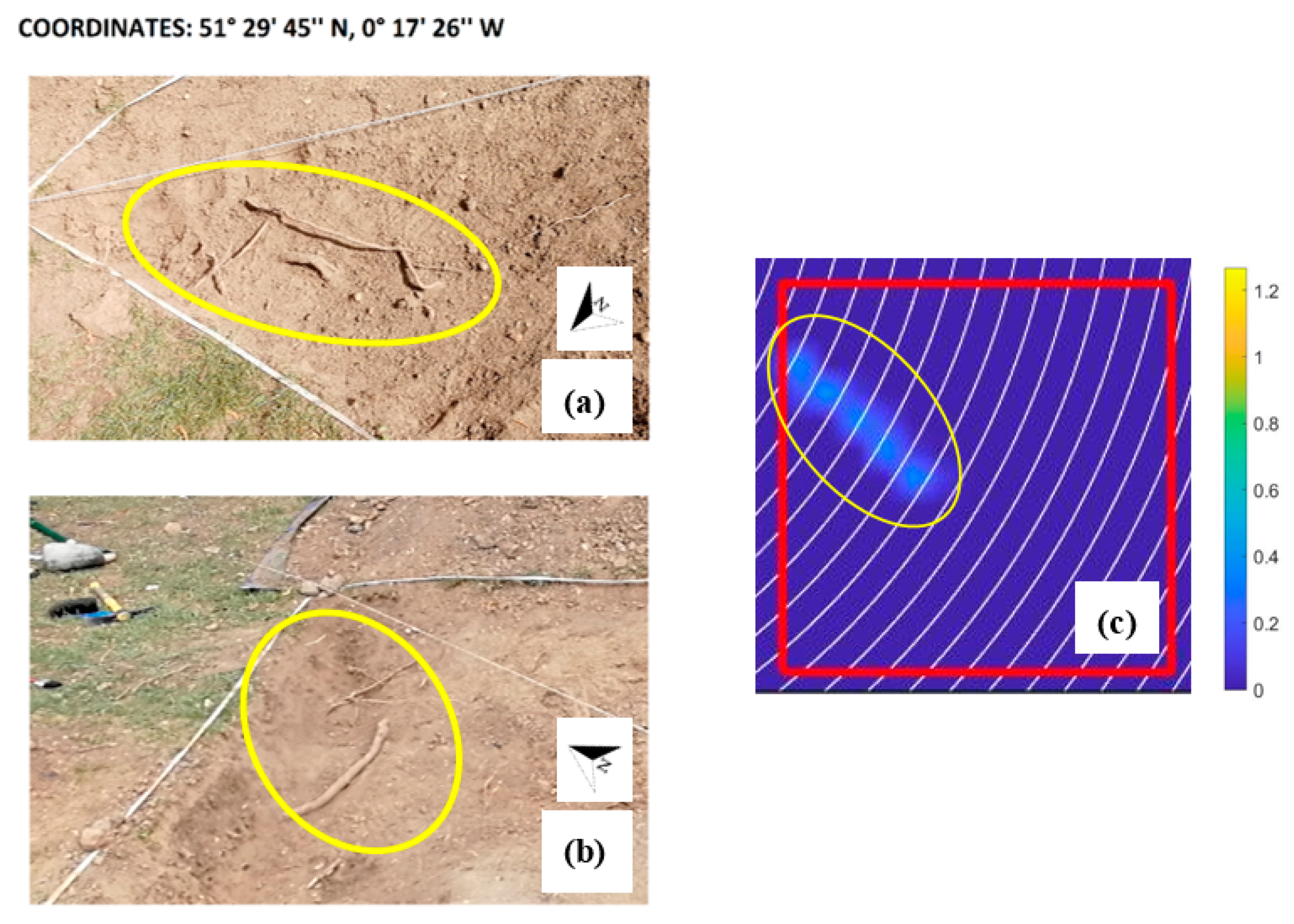
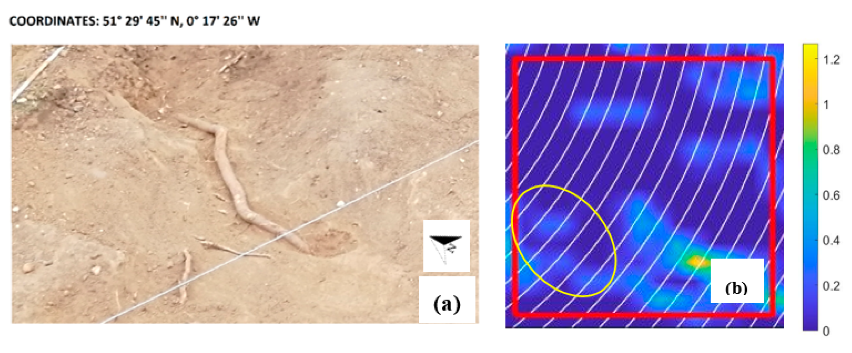
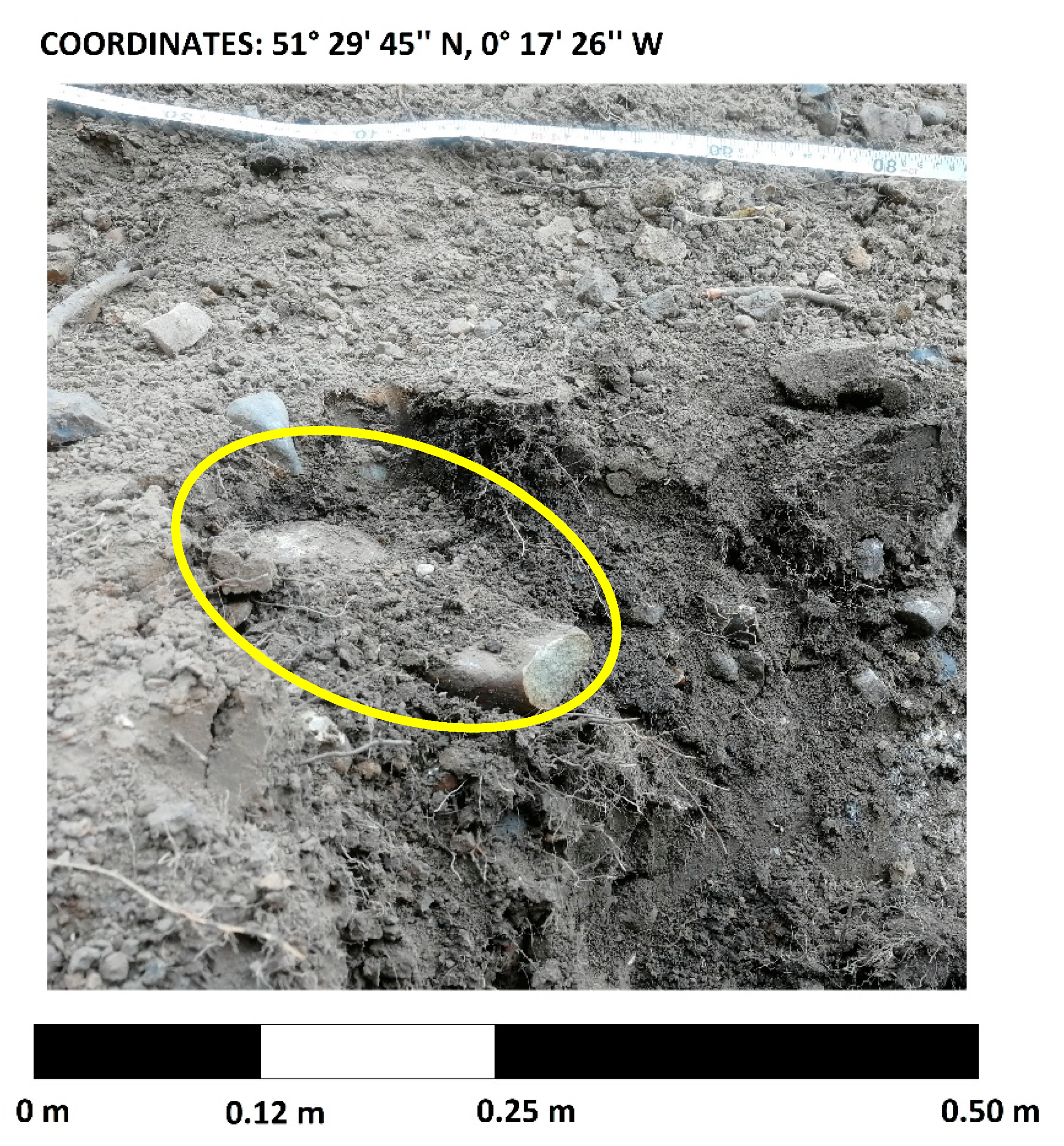
3.5. Results Validation through Excavation

A representative excavation section was identified after the application of the data processing framework in order to limit the validation stage to a useful portion of the overall investigated area (i.e., 218.04 m²).

A square area of 4 × 4 m was therefore selected on the South-West side of the investigated tree (Figure 16). The selection was made based on the root mass density distribution in the area and their expected depth. The excavation was performed by removing layers of ~0.10 m of soil up to ~0.50 m. It is worth noting that the soil was significantly dry and compact in the whole excavation area. Its removal therefore presented considerable difficulties, as the excavation had to be carried out with reduced size tools in order to ensure accurate operations and avoid accidental damage of the roots.

Several roots were found as a result of the validation survey, as shown in Figure 17. A root with an average diameter of 0.06 m crosses the bottom-right part of the excavation for a length of approximately 2.53 m, at a depth varying between 0.26 m and 0.50 m. However, a local increase in density was not found in the concerning density maps (i.e., depth ranges between 0.20 m and 0.30 m, between 0.30 m and 0.40 m, and between 0.40 m and 0.50 m). This is due to the particular orientation of the root that crosses the investigated area along the South-East—North-West direction, transversely to an imaginary radial line traced from the trunk of the tree investigated (Figure 18).

Given a typical configuration of a root system, where roots expand radially from the centre of the tree outwards, it is unlikely that the identified coarse root belongs to the tree under consideration. On the contrary, this root likely belongs to the tree located in the vicinity of the investigated one, as its direction matches with that conceivable for the nearby root system (see Figure 6). This result proves the validity of the proposed methodology in automatically excluding targets not belonging to the investigated tree.

A cluster of roots was also found at the top of the excavation area at a depth between approximately 0.20 m and 0.25 m. Its position matches with the outcomes of the map in the depth range 0.20 ÷ 0.30 m (Figure 19). Similarly, a root with an average diameter of 0.04 m was excavated at the top-right corner, and an evidence was again found in the 0.20–0.30 m density map.

Finally, the left-hand side of the excavation area was dug to validate the local density increase, as highlighted by Figure 20c and Figure 21c. Two roots with an average diameter of 0.04 m and a depth varying from 0.05 m (top-left corner) to 0.20 m (bottom-left corner) were excavated. Considering their position and the diameter similarity, it is reasonable to state that these sections belong to the same root that develops deeper than the performed excavation depth for a short stretch. As shown in Figure 20 and Figure 21, the development of the excavated roots resembles the outputs of the density maps. Lastly, roots of smaller dimensions, grouped together to form a single cluster, were found at a short distance from the two aforementioned roots (Figure 21a).

In addition, the presence of numerous boulders was detected (Figure 22), the main size of which exceeded 0.15 m in some cases. Some of the boulders were found along the top edge of the excavation area, whereas other boulders were found along the left edge.

However, no evidence of their presence was found in the root mass density maps. This confirms the validity of the proposed algorithm, as this is designed not to consider short segments, not correlated with root targets.

4. Discussion

The case study reported in this paper demonstrates the validity of the proposed methodology for the assessment of tree root systems. The method validation carried out through excavation and the subsequent roots exposure confirms that GPR can detect roots as well as that the presented data processing framework is able to reconstruct their pattern and provide crucial information on their mass density.

The data processing framework explained in Section 2.5.3 requires the input of a minimum amount of information related to the specific GPR survey, such as the number of scans carried out and the relative dielectric permittivity of the medium, making the data analysis relatively fast. Furthermore, the combination of the presented signal processing techniques allows for a broad applicability of the proposed methodology. A selection of standard techniques was performed to minimise the risk of data overprocessing. As for the more advanced techniques, such as the SVD filter and the F–K migration, their application has been calibrated to overcome fundamental issues, such as the presence of ringing noise and the accurate localisation of targets, without affecting the original data. The combination of the above-discussed parameters and processing steps can be regarded as a step forward for the development of a fully automated root system analysis methodology, for the use of practitioners and end-users. At present, the selection of the threshold value for use in the tree root-tracking algorithm is the only step requiring the operator’s intervention, as explained in Section 2.5.3. Future research could task itself towards the automation of this particular step, using iterative estimations [55] or machine-learning methods, such as the backpropagation [56].

Regarding the survey methodology, a circular GPR acquisition method was followed, as explained in Section 2.2 and Section 2.5.3. This method, chosen mainly due to the typical shape of a root system (i.e., expanding radially from the trunk of the tree outwards), has the advantage of being more inclusive and precise compared to a longitudinal acquisition method. In fact, circular transects enable scanning the roots in a quasi-perpendicular setup, i.e., an optimal condition in GPR data collection. Furthermore, this methodology is used to collect information related to the examined tree only, excluding the detection of root targets from neighbouring trees. This feature is essential for the evaluation of the root system of individual trees, in case more focused analyses are required. However, the circular acquisition turned up to be more time-demanding compared to traditional linear acquisitions. It is in fact fair to comment that, if the purpose of the survey relates to the assessment of multiple trees (e.g., a tree-lined avenue), the circular acquisition method is onerous and time-consuming. A desirable future prospect of the current research is therefore to adapt the discussed methodology into a linear acquisition method in order to facilitate the concurrent investigation of multiple nearby trees.

In regard to the outcomes produced by the tree root density maps, the evaluation of the mass density has proven to be an effective tool in assessing the root system conditions and its interaction with manmade constructions. To this extent, the provision of routine inspections could be of valuable support to evaluate the health conditions of root systems, as density variations over time can be used as an effective quantitative indicator of any potential diseases or fungal attacks. An early-stage identification of the problem could favour immediate remedial actions, and contribute to save the tree and prevent the spread of the infection. It is also worth noting the impact of the proposed methodology in large-scale forestry applications, especially in areas with a high density of trees. Implementation of routine inspections could help to identify mass density-related issues for individual trees (e.g., trees requiring special care) much more accurately, as the outcomes of the methodology are independent of the root system of nearby trees.

5. Conclusions

The present study clearly demonstrated that the use of non-destructive testing (NDT) methods for the investigation of tree root systems is the new frontier of forestry practices and the conservation of the naturalistic heritage. Due to its ease of use, non-intrusiveness and cost-effectiveness, the viability of the ground penetrating radar (GPR) technique was proven for root inspection purposes, with a special focus on root detection and the three-dimensional mapping of the root system architecture.

In this paper, the authors report an investigation within the context of forestry applications with GPR, aiming at detecting tree roots and reconstructing the geometry of a tree root system through a novel data processing methodology. A multi-stage interpretation algorithm was introduced in order to reconstruct the tree root patterns based on the collected GPR data. The proposed methodology is based on the provision of semi-circular scans, which expand outwards radially starting from the trunk of the tree. Initially, a signal processing stage was applied in order to remove noise-related information and enhance the response from the real targets. Subsequently, a tracking algorithm was used in order to locate and automatically track viable root paths. Lastly, the identified roots were expressed through continuous functions in order to map the root mass density analytically. A case study is presented in which the proposed method was successfully applied. The tracking algorithm has proven effective in identifying both the shallow (i.e., within the first 25 cm of soil) and the deep (i.e., below 25 cm from the surface of the soil) root structures. Based on this outcome, root mass density maps at different depths were estimated. To prove the validity of the proposed methodology, a validation survey was carried out, in which a part of the investigated area was excavated, and tree roots were exposed. The density maps were in good agreement with the actual root structure, as demonstrated by the orientation of the bigger roots excavated as well as by the presence of clusters of finer roots. In addition, the presence of boulders of appreciable size was not detected, although these features were found at several sections and depths within the excavated area. Finally, the proposed methodology has proven effective in mapping the root pattern and identifying mass density-related issues for individual trees, independently from the root systems of nearby trees.

It is believed that this research has contributed and added value to the existing knowledge within the context of understanding the conditions of tree roots in complex environments (e.g., urban environments), supporting the premise that GPR is a powerful NDT method for large-scale forestry applications.

References

1. Pallardy, S.G. Physiology of Woody Plants, 3rd ed.; Academic Press: Cambridge, MA, USA, 2010. [Google Scholar]
2. Donovan, G.H.; Butry, D.T.; Michael, Y.L.; Prestemon, J.P.; Liebhold, A.M.; Gatziolis, D.; Mao, M.Y. The relationship between trees and human health: Evidence from the spread of the emerald ash borer. Am. J. Prev. Med. 2013, 44, 139–145. [Google Scholar] [CrossRef] [PubMed]
3. Tzoulas, K.; Korpela, K.; Venn, S.; Yli-Pelkonen, V.; Kaźmierczak, A.; Niemela, J.; James, P. Promoting ecosystem and human health in urban areas using green infrastructure: A literature review. Landsc. Urban Plan. 2007, 81, 167–178. [Google Scholar] [CrossRef] [Green Version]
4. Tallis, M.; Taylor, G.; Sinnett, D.; Freer-Smith, P. Estimating the removal of atmospheric particulate pollution by the urban tree canopy of London, under current and future environments. Landsc. Urban Plan. 2011, 103, 129–138. [Google Scholar] [CrossRef]
5. Hwang, H.; Yook, S.; Ahn, K. Experimental investigation of submicron and ultrafine soot particle removal by tree leaves. Atmos. Environ. 2011, 45, 6987–6994. [Google Scholar] [CrossRef]
6. Mullaney, J.; Lucke, T.; Trueman, S.J. A review of benefits and challenges in growing street trees in paved urban environments. Landsc. Urban Plan. 2015, 134, 157–166. [Google Scholar] [CrossRef]
7. Hartig, T.; van den Berg, A.; Hagerhall, C.; Tomalak, M.; Bauer, N.; Hansmann, R.; Ojala, A.; Syngollitou, E.; Carrus, G.; van Herzele, A.; et al. Health benefits of nature experience: Psychological, social and cultural processes. In Forests, Trees and Human Health.; Nilsson, K., Sangster, M., Gallis, C., Hartig, T., de Vries, S., Seeland, K., Schipperijn, J., Eds.; Springer: Dordrecht, The Netherlands, 2011; pp. 127–168. [Google Scholar]
8. McPherson, E.G.; Nowak, D.J.; Rowntree, R.A. Chicago’s Urban Forest Ecosystem: Results of the Chicago Urban Forest Climate Project. Forest Service General Technical Report. U.S.; Department of Agriculture, Forest Service, Northeastern Forest Experiment Station: Washington, DC, USA, 1994. [Google Scholar]
9. Tyrväinen, L.; Pauleit, S.; Seeland, K.; de Vries, S. Benefits and uses of urban forests and trees. In Urban. Forests and Trees; Nilsson, K., Schipperijn, J., Randrup, T., Konijnendijk, C., Eds.; Springer: Berlin/Heidelberg, Germany, 2005; pp. 81–114. [Google Scholar]
10. Van Dillen, S.M.; de Vries, S.; Groenewegen, P.P.; Spreeuwenberg, P. Greenspace in urban neighbourhoods and residents’ health: Adding quality to quantity. J. Epidemiol. Community Health 2012, 66. [Google Scholar] [CrossRef] [PubMed] [Green Version]
11. Pandit, R.; Polyakov, M.; Sadler, R. The importance of tree cover and neighbourhood parks in determining urban property values. In Proceedings of the 56th Australian Agricultural and Resource Economics Society (AARES) Annual Conference, Fremantle, Australia, 7–10 February 2012. [Google Scholar] [CrossRef]
12. Coutts, M.P. Root architecture and tree stability. Plant Soil 1983, 71, 171–188. [Google Scholar] [CrossRef]
13. Alani, A.M.; Lantini, L. Recent advances in tree root mapping and assessment using non-destructive testing methods: A focus on ground penetrating radar. Surv. Geophys. 2020, 41, 605–646. [Google Scholar] [CrossRef]
14. Barton, C.V.M.; Montagu, K.D. Detection of tree roots and determination of root diameters by ground penetrating radar under optimal conditions. Tree Physiol. 2004, 24, 1323–1331. [Google Scholar] [CrossRef] [Green Version]
15. Hansen, E.M.; Goheen, E.M. Phellinus Weirii and other native root pathogens as determinants of forest structure and process in western north America. Annu. Rev. Phytopathol. 2000, 38, 515–539. [Google Scholar] [CrossRef]
16. Rishbeth, J. Resistance to fungal pathogens of tree roots. Proc. R. Soc. Lond. Ser. B. Biol. Sci. 1972, 181, 333–351. [Google Scholar] [CrossRef]
17. Shaw, C.G.; Kile, G.A. Armillaria Root Disease; Forest Service, US Department of Agriculture: Washington, DC, USA, 1991.
18. Reubens, B.; Poesen, J.; Danjon, F.; Geudens, G.; Muys, B. The role of fine and coarse roots in shallow slope stability and soil erosion control with a focus on root system architecture: A review. Trees 2007, 21, 385–402. [Google Scholar] [CrossRef]
19. Guo, L.; Chen, J.; Cui, X.; Fan, B.; Lin, H. Application of ground penetrating radar for coarse root detection and quantification: A review. Plant Soil 2013, 362, 1–23. [Google Scholar] [CrossRef] [Green Version]
20. Čermák, J.; Nadezhdina, N.; Meiresonne, L.; Ceulemans, R. Scots pine root distribution derived from radial sap flow patterns in stems of large leaning trees. Plant Soil 2008, 305, 61–75. [Google Scholar] [CrossRef]
21. Gregory, P.J.; Hutchison, D.J.; Read, D.B.; Jenneson, P.M.; Gilboy, W.B.; Morton, E.J. Non-invasive imaging of roots with high resolution X-ray micro-tomography. In Roots: The Dynamic Interface between Plants and the Earth; Abe, J., Ed.; Springer: Berlin/Heidelberg, Germany, 2003; pp. 351–359. [Google Scholar]
22. Moran, C.J.; Pierret, A.; Stevenson, A.W. X-Ray absorption and phase contrast imaging to study the interplay between plant roots and soil structure. Plant Soil 2000, 223, 101–117. [Google Scholar] [CrossRef]
23. Paglis, C.M. Application of electrical resistivity tomography for detecting root biomass in coffee trees. Int. J. Geophys. 2013, 2013, 6. [Google Scholar] [CrossRef]
24. Amato, M.; Basso, B.; Celano, G.; Bitella, G.; Morelli, G.; Rossi, R. In situ detection of tree root distribution and biomass by multi-electrode resistivity imaging. Tree Physiol. 2008, 28, 1441–1448. [Google Scholar] [CrossRef]
25. Benedetto, A.; Tosti, F.; Ortuani, B.; Giudici, M.; Mele, M. Soil moisture mapping using gpr for pavement applications. In Proceedings of the 2013 7th International Workshop on Advanced Ground Penetrating Radar, Nantes, France, 2–5 July 2013; pp. 1–5. [Google Scholar] [CrossRef]
26. Themistocleous, K.; Neocleous, K.; Pilakoutas, K.; Hadjimitsis, D.G. Damage assessment using advanced non-intrusive inspection methods: Integration of space, UAV, GPR, and field spectroscopy. In Proceedings of the Second International Conference on Remote Sensing and Geoinformation of the Environment (RSCy2014), Paphos, Cyprus, 7–10 April 2014; pp. 92291O-1–92291O-5. [Google Scholar] [CrossRef]
27. Hager, J.L.; Carnevale, M. GPR as a cost-effective bedrock mapping tool for large areas. In Proceedings of the Symposium on the Application of Geophysics to Engineering and Environmental Problems 2001, Denver, CO, USA, 4–7 March 2001; p. GP13. [Google Scholar] [CrossRef]
28. Daniels, D.J. Surface-penetrating radar. Electron. Commun. Eng. J. 1996, 8, 165–182. [Google Scholar] [CrossRef]
29. Goodman, D. Ground-penetrating radar simulation in engineering and archaeology. Geophysics 1994, 59, 224–232. [Google Scholar] [CrossRef]
30. Alani, A.M.; Aboutalebi, M.; Kilic, G. Applications of ground penetrating radar (gpr) in bridge deck monitoring and assessment. J. Appl. Geophys. 2013, 97, 45–54. [Google Scholar] [CrossRef]
31. Potin, D.; Duflos, E.; Vanheeghe, P. landmines ground-penetrating radar signal enhancement by digital filtering. IEEE Trans. Geosci. Remote Sens. 2006, 44, 2393–2406. [Google Scholar] [CrossRef] [Green Version]
32. Tosti, F.; Bianchini Ciampoli, L.; D’Amico, F.; Alani, A.M.; Benedetto, A. An experimental-based model for the assessment of the mechanical properties of road pavements using ground-penetrating radar. Constr. Build. Mater. 2018, 165, 966–974. [Google Scholar] [CrossRef]
33. Brancadoro, M.G.; Ciampoli, L.B.; Ferrante, C.; Benedetto, A.; Tosti, F.; Alani, A.M. An investigation into the railway ballast grading using gpr and image analysis. In Proceedings of the 2017 9th International Workshop on Advanced Ground Penetrating Radar (IWAGPR), Edinburgh, UK, 28–30 June 2017; pp. 1–4. [Google Scholar] [CrossRef]
34. Lambot, S.; Javaux, M.; Hupet, F.; Vanclooster, M. A global multilevel coordinate search procedure for estimating the unsaturated soil hydraulic properties. Water Resour. Res. 2002, 38, 6–15. [Google Scholar] [CrossRef]
35. Huisman, J.A.; Hubbard, S.S.; Redman, J.D.; Annan, A.P. Measuring soil water content with ground penetrating radar: A review. Vadose Zone J. 2003, 2, 476–491. [Google Scholar] [CrossRef]
36. Hruska, J.; Čermák, J.; Šustek, S. Mapping tree root systems with ground-penetrating radar. Tree Physiol. 1999, 19, 125–130. [Google Scholar] [CrossRef] [Green Version]
37. Butnor, J.R.; Doolittle, J.A.; Johnsen, K.H.; Samuelson, L.; Stokes, T.; Kress, L. Utility of ground-penetrating radar as a root biomass survey tool in forest systems. Soil Sci. Soc. Am. J. 2003, 67, 1607–1615. [Google Scholar] [CrossRef] [Green Version]
38. Alani, A.M.; Ciampoli, L.B.; Lantini, L.; Tosti, F.; Benedetto, A. Mapping the root system of matured trees using ground penetrating radar. In Proceedings of the 2018 17th International Conference on Ground Penetrating Radar (GPR), Rapperswil, Switzerland, 18–21 June 2018; pp. 1–6. [Google Scholar] [CrossRef]
39. Lantini, L.; Holleworth, R.; Egyir, D.; Giannakis, I.; Tosti, F.; Alani, A.M. Use of ground penetrating radar for assessing interconnections between root systems of different matured tree species. In Proceedings of the 2018 Metrology for Archaeology and Cultural Heritage (MetroArchaeo), Cassino, Italy, 22–24 October 2018; pp. 22–26. [Google Scholar] [CrossRef]
40. Gunnersbury Park Trees. Available online: https://gunnersburyfriends.org/gunnersbury-park-trees/ (accessed on 15 July 2020).
41. Time and Date AS. Available online: https://www.timeanddate.com/weather/uk/london/historic?month=4&year=2019 (accessed on 3 July 2020).
42. Fayle, D.C.F. Radial growth in tree roots: Distribution, Timing, Anatomy; University of Toronto, Faculty of Forestry: Toronto, ON, Canada, 1968. [Google Scholar]
43. Chauvière, M.; Colin, F.; Nielsen, C.N.; Drexhage, M. Development of Structural Root Architecture and Allometry of Quercus Petraea. Can. J. For. Res. 1999, 29, 600–608. [Google Scholar] [CrossRef]
44. Elkarmoty, M.; Tinti, F.; Kasmaeeyazdi, S.; Giannino, F.; Bonduà, S.; Bruno, R. Implementation of a fracture modeling strategy based on Georadar Survey in a large area of Limestone Quarry Bench. Geosciences 2018, 8, 481. [Google Scholar] [CrossRef] [Green Version]
45. Daniels, D.J. Ground Penetrating Radar, 2nd ed.; The Institution of Electrical Engineers: London, UK, 2004. [Google Scholar]
46. Jol, H.M. Ground Penetrating Radar Theory and Applications, 1st ed.; Elsevier: Amsterdam, The Netherlands, 2009. [Google Scholar]
47. Kim, J.; Cho, S.; Yi, M. Removal of ringing noise in GPR data by signal processing. Geosci. J. 2007, 11, 75–81. [Google Scholar] [CrossRef]
48. Lantini, L.; Giannakis, I.; Tosti, F.; Mortimer, D.; Alani, A. A reflectivity-based gpr signal processing methodology for mapping tree root systems of street trees. In Proceedings of the 2020 43rd International Conference on Telecommunications and Signal Processing, Budapest, Hungary, 7–9 July 2020. [Google Scholar] [CrossRef]
49. Cui, X.H.; Chen, J.; Shen, J.; Cao, X.; Chen, X.; Zhu, X. Modeling tree root diameter and biomass by ground-penetrating radar. Sci. China Earth Sci. 2011, 54, 711–719. [Google Scholar] [CrossRef]
50. Kreyszig, E. Advanced Engineering Mathematics, 9th ed.; John Wiley & Sons: Hoboken, NJ, USA, 2006. [Google Scholar]
51. Hansen, P.C.; Pereyra, V.; Scherer, G. Least Squares Data Fitting with Applications; Johns Hopkins University Press: Baltimore, MD, USA, 2013. [Google Scholar]
52. Fausett, L.V. Applied Numerical Analysis using MATLAB, 2nd ed.; Pearson Prentice Hall: Upper Saddle River, NJ, USA, 2008. [Google Scholar]
53. Köstler, J.; Brückner, E.; Bibelriether, H. Die Wurzeln Der Waldbäume; P. Parey: Hamburg, Germany, 1968. [Google Scholar]
54. Crow, P. The influence of soils and species on tree root depth. For. Comm. 2005, 1–8. [Google Scholar]
55. Kelley, C.T. Iterative Methods for Optimization; Society for Industrial and Applied Mathematics: Philadelphia, PA, USA, 1999. [Google Scholar]
56. Hecht-Nielsen, R. Theory of the backpropagation neural network. Neural Netw. 1988, 1, 445. [Google Scholar] [CrossRef]
Figure 1. Study site for the GPR investigation (map data: Google, Landsat/Copernicus).
Remotesensing 12 03417 g001
Figure 2. Detail of the survey setup.
Remotesensing 12 03417 g002
Figure 3. Rendering of the GPR survey setup.
Remotesensing 12 03417 g003
Figure 4. Verification of the accuracy of the excavation area’s coordinates. Note that the tree was felled before the excavation stage (the trunk base is visible on the left-hand side of the picture).
Remotesensing 12 03417 g004
Figure 5. Flowchart of the tree root-tracking algorithm’s iterative procedure.
Remotesensing 12 03417 g005
Figure 6. Layout of the roots’ main directions in the case of two adjacent trees. Directions of roots of a reference tree (e.g., the tree under investigation in this study) (in green) are not compatible with the roots’ directions of a nearby adjacent tree (in red).
Remotesensing 12 03417 g006
Figure 7. B-scan (a) before the application of the preliminary signal processing stage, (b) after the application of standard signal processing and SVD filter, and (c) after the application of the F–K migration.
Remotesensing 12 03417 g007
Figure 8. A B-scan showing the presence of a buried structure (highlighted by the red dashed square).
Remotesensing 12 03417 g008
Figure 9. C-scans of the investigated area at (a) 0.31 m of depth and (b) 0.45 m of depth. The red dashed areas clearly show the presence of a buried structure.
Remotesensing 12 03417 g009
Figure 10. Aerial view of the investigated area. The red dashed area highlights a difference in the ground appearance matching the identified location of the discontinuity feature.
Remotesensing 12 03417 g010
Figure 11. An example of the GPR reflectivity analysis. (a) B-scan after the preliminary signal processing stage, (b) analysis of the signal reflectivity, showing a maximum value at the section coordinates of the identified buried feature, and (c) B-scan after a targeted trace removal.
Remotesensing 12 03417 g011
Figure 12. Reconstructed map of the tree root system architecture: (a) 2D planar view, (b) 3D view from South-West, and (c) in a 3D view from North-West. The grey block represents the volume occupied by the buried feature.
Remotesensing 12 03417 g012
Figure 13. Root mass density maps at different depths: (a) from 0 m to 0.10 m, (b) from 0.10 m to 0.20 m, and (c) from 0.20 m to 0.30 m.
Remotesensing 12 03417 g013
Figure 14. Root mass density maps at different depths: (a) from 0.30 m to 0.40 m, (b) from 0.40 m to 0.50 m, and (c) from 0.50 m to 0.60 m.
Remotesensing 12 03417 g014
Figure 15. Root mass density map from 0.60 m to 0.70 m.
Remotesensing 12 03417 g015
Figure 16. Rendering of the surveyed area, showing the position of the excavated site.
Remotesensing 12 03417 g016
Figure 17. The excavated site.
Remotesensing 12 03417 g017
Figure 18. An outline of the survey, showing the orientation of the excavated coarse root (in red) within the test pit area.
Remotesensing 12 03417 g018
Figure 19. (a) The excavated root cluster, and (b) a close-up view of the 0.20–0.30 m density map. The yellow circle highlights an area with increased density, corresponding to the cluster of roots.
Remotesensing 12 03417 g019
Figure 20. The excavated root at the top-left corner of the excavated area, (a) detail of the excavation, (b) development of the root, and (c) a close-up view of the 0.10–0.20 m density map. The yellow circle highlights an area with an increased density, corresponding to the excavated root.
Remotesensing 12 03417 g020
Figure 21. The excavated root at the bottom-left corner of the excavated area, (a) development of the root, and (b) a close-up view of the 0.20–0.30 m density map. The yellow circle highlights an area with an increased density, corresponding to the excavated root.
Remotesensing 12 03417 g021
Figure 22. Boulders found along the top edge of the excavation area. The boulder in the foreground has a main axial dimension of approximately 0.15 m.
Remotesensing 12 03417 g022