Recent Crustal Deformation Based on Interpolation of GNSS Velocity in Continental China

1
College of Surveying and Geo-Informatics, Tongji University, Shanghai 200092, China
2
Key Laboratory of Earthquake Prediction, China Earthquake Administration, Beijing 100036, China
*
Author to whom correspondence should be addressed.
Remote Sens. 2020, 12(22), 3753; https://0-doi-org.brum.beds.ac.uk/10.3390/rs12223753
Submission received: 19 October 2020
/
Revised: 9 November 2020
/
Accepted: 13 November 2020
/
Published: 14 November 2020
(This article belongs to the Special Issue GNSS for Geosciences)
Abstract
:We used the interpolation method of two-dimensional vector velocity field data based on Green’s function to conduct coupled interpolation with a Poisson’s ratio of 0.5 for 1966 horizontal velocity field data from 1999 to 2017 and obtained the uniform velocity field and strain rate field with a grid of 1°. The main results are as follows: the eastern Himalayan structure as the center, the eastern Lhasa block, the eastern Qiangtang block, the Sichuan-Yunnan block, and the Burma block form a strong deformation rate zone of continuous deformation in the fan-shaped region, which has been a strong deformation rate zone for earthquakes of magnitude 7 or higher in continental China since 1963. Besides, the eastward movement of crustal material in the Tibetan Plateau is blocked by the stable South China block. Therefore, the direction of crustal material movement is deflected, which gradually forms a clockwise rotation motion system centered on the eastern Himalayan structure. Finally, our research shows that the influencing factors of strong earthquakes include velocity change, non-uniform strain distribution, accumulation of larger strain, and the difference of the second strain rate invariant. Strong earthquakes are closely related to the difference in energy accumulation in space.
1. Introduction
Located in the southeast of the Eurasian plate, sandwiched between the Indo-Pacific plate and the Philippine Sea plate, China is an area of strong late quaternary and modern tectonic activity. Under the interaction of the Indian Ocean plate, the Pacific Plate, the Eurasian Plate, and the Pacific Plate, as well as the action of the deep earth dynamics within the Eurasian plate, continental China has a unique spatial distribution pattern of strong earthquakes. China is a region with the strongest earthquakes in the global continent (Figure 1), and 33% of the earthquakes in the global continent occur in continental China [1]. Urban earthquake disaster is particularly prominent, which brings a great threat to people’s lives and the development of civilization. Therefore, understanding the laws of block movement and crustal deformation plays a great role in the study and prediction of earthquakes, and at the same time, it can reduce the adverse effects of earthquake disasters to a certain extent [2].
The collision between the Indian Plate and the Eurasian Plate caused a large-scale crustal deformation and crustal motion of continental China (Figure 1). Researchers have studied the characteristics of tectonic movement in continental China, such as crustal shear deformation, crustal expansion and subtraction, crustal rotation deformation, and fault movement [3,4,5,6,7]. Furthermore, many scholars have evaluated the tectonic activity and seismic activity of continental China [8,9,10,11,12,13,14,15]. Nowadays, there are two models of crustal deformation, “block model” [12,13] and “continuous model” [14,15]. The block model is mainly proposed by geologists, who believe that most of the deformation occurs along the main block boundary fracture. On the other hand, the continuous model is mainly proposed by geophysicists, who believe that the deformation is quasi-continuous, subject to the solid flow of viscous material similar to fluid control.
With the rapid progress of Global Navigation Satellite System (GNSS) technology, as well as the continuous improvement of GNSS accuracy and space-time resolution, GNSS has gradually become an essential observation means in geoscience research, especially in crustal deformation research. Deformation research based on GNSS is ongoing, which provides a data reference basis for the different scales of subsequent deformation research [16,17,18,19,20,21,22,23,24,25,26,27,28,29,30]. Although many scholars have studied the velocity field data of GNSS stations, with the increasing time span of the data, previous studies have a certain timeliness.
The interpolation of velocity field data of GNSS stations can produce a continuous strain rate field without any assumption of the deformation mechanism. For this reason, researchers proposed a variety of data interpolation schemes. Kahle [31] interpolated the velocity fields in the eastern Mediterranean using the least square configuration method based on the covariance function. Wdowinski [32] interpolated the velocity field along a small circle relative to the rotating pole to minimize the residual error. Allmendinger [33] used different methods (nearest neighbor method and distance weighting method) to obtain a continuous velocity field, from which strain rate can be calculated. Shen [34] used neighborhood weighting and least square inversion estimation parameters to obtain interpolation algorithms, and obtained continuous velocity field, and calculated strain rate. However, these interpolation methods cost a lot of time and the process is relatively complex. Generic Mapping Tools (GMT) is one of the most widely used open-source free mapping software in earth science, with powerful mapping function and data processing function. In terms of data processing, GMT has such functions as data screening, resampling, time-series filtering, two-dimensional grid filtering, three-dimensional grid interpolation, polynomial fitting, linear regression analysis, and so on. Besides, GMT can be used to achieve rapid and convenient interpolation and strain rate calculations [35].
In this study, we used the interpolation method of two-dimensional vector velocity field data based on Green’s function to conduct coupled interpolation with a Poisson’s ratio of 0.5 for 1966 horizontal velocity field data of GNSS stations from 1999 to 2017 and obtained the uniform velocity field with a grid of 1°. By taking the partial derivative of the velocity field, the continuous and uniform strain rate is obtained and achieved the fast and convenient interpolation, and strain rate calculation. Besides, cross-validation error analysis is also carried out for the interpolated velocity field results. This paper also uses the strain rate results to analyze the movement mode and strain rate distribution law of different active blocks in continental China and compares the tectonic characteristics of active blocks, and we compared the correlation between the tectonic characteristics of active blocks and the occurrence of strong earthquakes.
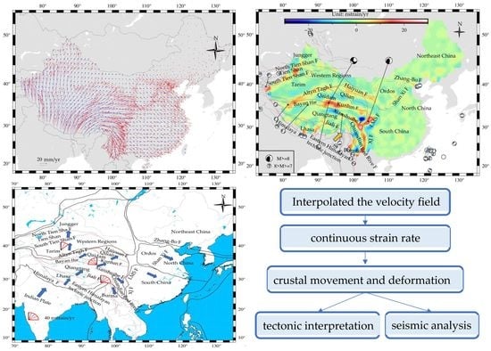
The aim of this paper is to analyze the current crustal movement and deformation field in continental China for tectonic interpretation and seismic analysis. In Section 2, we briefly introduce the data of GNSS stations processed in this paper and review the velocity field interpolation and strain calculation methods. In Section 3, based on the results of velocity field interpolation and strain distribution, we discuss the motion patterns and strain distribution laws of different active blocks in continental China. Besides, error analysis is also carried out. In Section 4, we compare the historical tectonic characteristics of the active block with the historical seismic frequency for tectonic interpretation and seismic analysis. In Section 5, we give conclusions of this paper.
2. Materials and Methods
2.1. Data
A total of 2765 observation stations were collected from 8 GNSS networks (Table 1) in continental China and its adjacent areas, including 490 continuous stations and 2275 staging stations. The GNSS network is processed on Bernese 5.2 software, and the daily solution of GNSS station positions is computed via the minimal constraint approach. Besides, Finite Element Solutions 2004 (FES2004) ocean tidal loading corrections [36], atmosphere S1–S2 tidal loading corrections [37], and absolute phase-center corrections for satellites and receivers, as issued by International GNSS Service (IGS) [38], were applied to the formulation of the observation equations. Furthermore, the controlled datum removal filtering method was employed to remove noise.
The GNSS station coordinate time series fitting function model adopts the extended model proposed by Bevis and Brown [32]. GNSS station coordinates time series fitting adopts the least-squares method, noise analysis adopts Maximum Likelihood Estimation (MLE) method, and at the same time, the fitting model parameters and noise model parameters of GNSS station coordinate time series are estimated. Furthermore, using the Gaussian inverse distance weighting method, the original GNSS station coordinate time series are respectively interpolated with an annual period, semi-annual period, earthquake co-seismic and post-seismic signal interpolation, and the interpolation model value is directly deducted from the rover coordinate time series. Besides, the noise of the station can also be obtained and deducted by the method of continuous station noise interpolation or averaging. Eventually, the corrected GNSS station coordinate time series is obtained. For more details, refer to Weiwei Wu’s thesis [39].
Using the Bernese 5.2 software networking solutions for calculating all the observational data, obtained the GNSS station coordinate time series. The velocity field of the GNSS station is obtained by analyzing the coordinate time series of the station. The results showed that the average error in the horizontal velocity field is about 0.2~0.3 mm/yr, and the average error in the vertical velocity field is about 0.5 mm/yr [39,40].
According to the principle that error is less than 2.0 mm/yr, we selected 1966 horizontal velocity field data from the velocity field in the GNSS stations, and to eliminate some of the data. For example, in order to avoid the short wave mixing in the process of interpolation and the adverse effects of abnormal data, every 30 arc minute has carried on the weighted average of the data processing. Besides, we also eliminated the data with an error greater than twice the median error and the data with a significant deviation of the velocity direction from the overall motion trend.
2.2. The Interpolation
The main purpose of interpolation is that we wanted to use discrete GNSS station data to obtain the continuous strain rate field of the crust. The green’s function method of 2-D vector data interpolation in GMT is used for data coupling interpolation [41]. It is similar to the double harmonic spline interpolation method and used the 2-D elastic model to provide the coupling between two horizontal velocity components of data. The principle of coupling interpolation is to apply a plane vector force at the location of the data so that the elastomer deforms and a vector deformation field is formed. The magnitude and direction of the force applied will be adjusted continuously until it is in a better match with the known velocity vector data. Finally, the velocity field can be obtained at any location. The coupling interpolation realizes the plane response of the two-dimensional elastomeric body to plane stress by analyzing Green’s function. By adjusting Poisson’s ratio, the strain field can be adjusted to different extreme cases of incompressibility, typical elasticity, and complete compression. Through the plane stress of the response, any position vector velocity field is obtained by inversion, and then data interpolation is carried out.
The size of the grid has a non-negligible influence on the interpolation result. Too fine grid size will lead to a highly irregular strain rate graph, high strain rate peak appears at the observation point, and at the same time may cause the interpolation tension to increase. We noticed that many artifacts are introduced in such interpolation. Too coarse grid size results in an inferior and highly localized strain rate. Ideally, each cell should have at least one observation point [42]. Therefore, based on the distribution of GNSS observations, a regular grid with a lattice size of 1° is selected to interpolate the components of the horizontal velocity field in continental China.
In the process of interpolation data processing, a mask of the research area was first established, and the processed horizontal velocity field data were interpolated within the mask by 1° × 1°. Poisson’s ratio 0.5, which represents typical elasticity, was selected. After interpolation, two continuous scalar fields are obtained, namely, the velocity component in the east direction and the velocity component in the north direction in the study area.
2.3. Calculation of Strain Rate
If the crust is thought of as an elastomer, the strain or strain rate can be calculated from the observed displacement or velocity. The strain tensor of the earth’s surface can be expressed as a partial derivative of displacement in spherical coordinates [16,43]. The methods of strain rate calculation are divided into segment approach and gridded approaches. The segment approach divides the research area into several segments and takes subnets as the unit to first calculate the strain parameters of each segment. Finally, all the individual results are integrated to calculate the uniform strain rate within the subnet. For example, Savage [43] calculated the strain rates of different blocks in the northwestern United States by using the Taylor expansion formula of spherical displacement and strain obtained by the Taylor series. Besides, the Delaunay triangle method is a typical segment approach [44]. However, the disadvantages of these methods are obvious. Generally speaking, there is no data redundancy, so outliers cannot be detected and removed. Besides, their resultant strain rates are also discontinuous.
The study area is divided into uniform grids by the gridded approaches. Firstly, the displacement function of all stations is fitted into one displacement field function, and then the partial derivative at the grid point is calculated to obtain the strain field distribution directly. The displacement determined by gridded approaches is mainly based on statistical analysis. It assumes that the displacement field can be decomposed into the parametric part of the system and the random signal part, and the constructor of the signal part can be determined by statistical methods. The gridded approaches include the multi-quadric function method, spherical harmonic function method, and least square collocation method [42,45]. These strain calculation methods have different applicability for different research purposes and data sparsity. However, they are all suitable for inversion problems. For instance, according to the distance of measuring point velocity field near the weighted, Shen [45] used the least square collocation method to solve the grid point of strain rate using the weighted velocity field data, and finally obtained the strain rate field in California area; Hackl [42] first projected the velocity field parallel to the fault and perpendicular to the fault and used Green’s function to conduct spline curve interpolation to form a uniform grid, and then took the derivative of the spline function to calculate the strain rate field in the southern California region of the United States.
We referred to the method of calculating the strain rate published by Hackl [42] that it can be calculated the velocity gradient by using the spatial partial derivative of the interpolation velocity field, and we obtained the strain rate component. Afterward, the derivatives along the local north direction and east direction can be calculated to generate four continuous fields, which can represent a continuous strain rate tensor in a linear combination. Assuming that there was a small deformation, in the case that GMT can be automatically converted into geographical coordinates for calculation, the component of the strain rate tensor was calculated as shown in Equation (1) [42]:
where represents latitude, represents longitude, and represent the velocity of a point in the direction of longitude and latitude, and , , and represent the three independent strain rate components of the strain rate tensor.
The maximum and minimum principal strains are calculated as Equation (2):
where represents the maximum principal strain and represents the minimum principal strain.
The maximum shear strain rate and its direction may provide a tool for identifying active faults since movement along the fault is associated with shear on the structure. In an earthquake event, a fault in this direction is most likely to rupture. The maximum shear strain rate of each grid point can be obtained by a linear combination of the maximum eigenvalue and the minimum eigenvalue. The maximum shear strain rate () is calculated by Equation (3):
The dilation rate is considered as the representative of horizontal deformation related to the dip-slip fault. The dilation rate () is calculated by Equation (4):
The rotation rate () Equation (5) is as follows:
The second strain rate invariant depicts the energy characteristics of regional crustal deformation. The second strain rate invariant () Equation (6) is as follows:
3. Results
According to geological data [46], continental China contains six first-grade active blocks, namely Northeast Asia block, North China block, South China block, Burma block, Tibetan block, and Western Regions block. The Tibet block contains secondary blocks, which are the Lhasa block, the Qiangtang block, the Sichuan-Yunnan block, the Bayan Har block, the Qaidam block, and the Qilian block. The Western Region Block contains secondary blocks, which are Tianshan Block, Tarim Block, and Junggar Block, and so on. In this study, the Northeast Asia block, the North China block, and the South China block belong to eastern China, and the Burma block, the Tibetan block, and the Western Regions block belong to western China.
We calculated the range and mean value of the strain rate index of first-grade blocks in continental China (Table 2). In this paper, the nstrain/yr stands for 10−9 strain/yr. Besides, based on the results of velocity field interpolation and strain distribution, we discuss the motion patterns and strain distribution laws of different active blocks in continental China.
3.1. Interpolation
The interpolation method in Section 2.2 is adopted to obtain the horizontal velocity field of the 1-degree grid in continental China by using GMT. The interpolation results of the velocity field in continental China are shown in Figure 2.
As Figure 2 shows, the spatial distribution of the measured velocity field of the horizontal crustal movement in continental China is uneven and has obvious zoning characteristics. From the analysis of the measured velocity field numerical value, the velocity field numerical value in the west is large, while the velocity field numerical value in the east is small. The velocity field in the west is decreasing from south to north. In the eastern velocity field, the velocity numerical values of the active blocks in Southeast Asia are small, while the velocity numerical values of the rest blocks are relatively average. On the other hand, from the aspect of motion direction analysis, there is a consistent north-to-north-east motion in the west, while a consistent south-easterly motion in the east. Except for the active block in Northeast Asia, due to the short observation time of each station in the Northeast Asia block, the error may be large, and the overall trend of velocity field motion direction moves clockwise from west to east.
3.2. Strain Rate
3.2.1. Principal Strain Rate
We use the strain rate calculation method in Section 2.3 to interpolate the horizontal velocity field, and obtained the horizontal principal strain rate distribution results in continental China.
As Figure 3 and Table 2 shows, just like the horizontal velocity field interpolation diagram, the principal strain rate distribution diagram also appears as an obvious non-uniform spatial distribution with an obvious partitioning feature.
The principal strain rate in western China is much larger than that in eastern China. In the western part of continental China, the value of the principal strain rate is larger, and the strain distribution is more complex, which indicates that there are more intense crustal deformation and more complex geological tectonic movement in the region; In the eastern part of continental China, the overall value of the principal strain rate is small, and the average value of the three active blocks in the eastern part is all less than 5.00 nstrain/yr. The direction of the principal strain rate varies significantly in the eastern part of continental China, most of the overall direction is the main pressure from northeast to southwest and the main pull from northwest to southeast.
According to Figure 3 and Table 2, we find that the regions with higher principal strain rates are mainly concentrated in the Tibetan block, the Burma block, the Tien Shan block, and the areas near the southern boundary of the Tien Shan block. Besides, with the eastern Himalayan tectonic junction as the center, a continuous strong deformation zone is formed in the fan-shaped region between the eastern Himalayan tectonic junction, the Sichuan-Yunnan block, the Burma block, the Bayan Har block, the Qaidam block, the eastern part of the Lhasa block and the eastern part of the Qiangtang block.
3.2.2. The Other Strain Rate
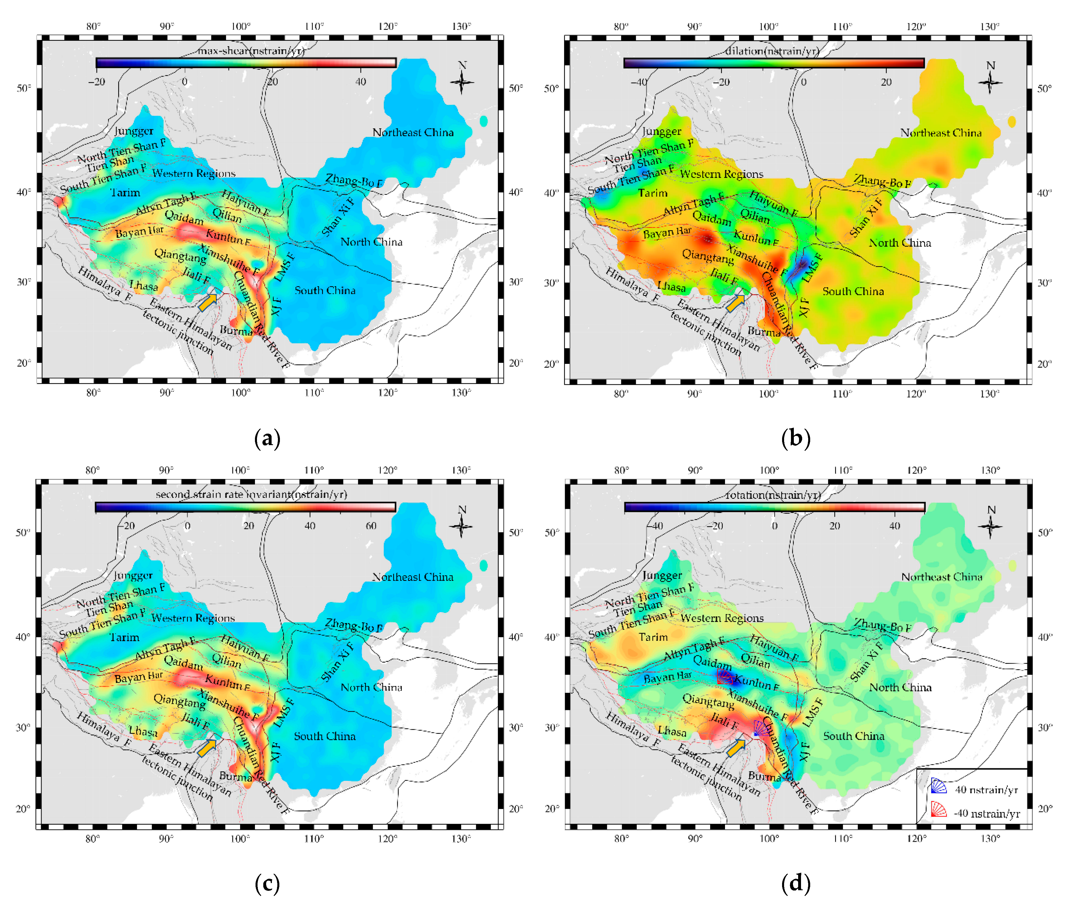
We mainly introduce the distribution of maximum shear strain rate, dilation rate, rotation rate in continental China (Figure 4). The distribution of the maximum shear strain rate field (Figure 4a) has the following characteristics. The maximum shear strain rate field shows a regional distribution characteristic similar to the maximum principal strain rate field. The larger value of the principal strain rate field also shows a larger maximum shear strain rate. Generally speaking, the maximum shear strain rate values in the eastern part of China are very small, and the overall crustal shear deformation is feeble. On the contrary, the western part of China shows a large maximum shear strain rate.
According to the results of the maximum shear strain rate and Table 2, on the one hand, the maximum shear strain rate characteristics of the Northeast Asia block, the North China block, and the South China block are not obvious, and the average maximum shear strain rate does not exceed 5.00 nstrain/yr. Only in the Zhang-Bo fault zone and Shan Xi fault zone, the maximum shear strain rate is larger than 10 nstrain/yr, and the maximum value reaches 25.86 nstrain/yr, indicating that the crustal shear deformation in these two areas is relatively obvious. On the other hand, the maximum shear strain rate of the Tibetan block, the Tien Shan block, and the Burma block are strong. The maximum shear strain rate range of the Tibetan block about 1.04~47.68 nstrain/yr. The maximum shear strain rate increases continuously from the Himalayan main thrust zone to the Jiali fault zone and then to the Xianshuihe fault zone, until the maximum shear strain rate appears near the Kunlun fault zone, reaching 47.68 nstrain/yr. From the Kunlun fault zone to the Altyn Tagh fault zone and Haiyuan fault zone, the maximum shear strain rate decreases first and then increases from south to north. In the Altyn Tagh fault zone and Haiyuan fault zone, the strain rate is larger. In the western region block, the maximum shear strain rate near the Tien Shan fault zone is greater than 21.00 nstrain/yr. Therefore, it shows that there is strong shear deformation around the Altyn Tagh fault zone, the Haiyuan fault zone, the Tien Shan fault zone, the Kunlun fault zone, Jiali fault zone, and Xianshuihe fault zone. The maximum shear strain rate is large in most areas of the Burma block, and the average maximum shear strain rate is about 21.01 nstrain/yr. A strong shear strain is common in this area.
The distribution of the dilation rate field (Figure 4b) has the following characteristics. There are obvious characteristics of dilatational strain in the western part of China. However, the characteristics of dilatational strain are not obvious in the eastern part of China.
According to the results of the dilation rate and Table 2, the average dilation rate of the Northeast Asia block, the North China block, and the South China block is lower than 2.22 nstrain/yr, so the characteristics of dilatational strain are not obvious. On the contrary, there are obvious characteristics of compressive strain between the Himalayan fault zone and the JiaLi fault zone, and there are obvious characteristics of dilatational strain from the JiaLi fault zone to the Xianshuihe fault zone and then to the Kunlun fault zone. Moreover, it appears obvious characteristics of compressive strain again between the Kunlun fault zone and the Altyn Tagh fault zone. We infer that there is an obvious expansion belt in the Tibetan block.
The dilation rate of the Western Region block ranges from −31.79~7.39 nstrain/yr, showing obvious characteristics of compressive strain. Among them, the compression rate of the Tien Shan block and its boundary is as high as 20.22 nstrain/yr. The average dilation rate of the Burma block is about 7.78 nstrain/yr, showing obvious characteristics of the dilatational strain.
The distribution of the second strain rate invariant (Figure 4c) has the following characteristics, it is highly consistent with the principal strain rate and the maximum shear strain rate, and large second strain invariants also appear in the regions with large values of the principal strain rate field. According to the results of the dilation rate and Table 2, the average second strain rate invariant of the Tien Shan block, the Tibetan block, and the Burma block are as high as 25.62 nstrain/yr, 26.32 nstrain/yr, and 30.86 nstrain/yr, respectively. Because the second strain invariant depicts the energy characteristics of regional crustal deformation and reveals the crustal deformation regions with relatively obvious seismic zones, these three regions are highly prone to earthquakes.
For the distribution characteristics of the rotation rate field (Figure 4d), in the western part of China, a fan unit with the eastern Himalayan tectonic junction as the center of continuous deformation appears. However, in the eastern part of China, the rotation rate value has small fluctuation and relatively uniform distribution, and there is no salient feature on the whole.
The results show that the rotation characteristics of the Northeast Asia block, the North China block, and the South China block are not obvious. However, Tibetan block and Burma block has a strong rotation rate. With the eastern Himalayan tectonic junction as the center, a continuous strong deformation zone is formed in the fan-shaped region between the eastern Himalayan tectonic junction, the Sichuan-Yunnan block, the Burma block, the Bayan Har block, the Qaidam block, the eastern part of the Lhasa block and the eastern part of the Qiangtang block. The closer distances from the center of the fan-shaped region, the greater the rate of change of clockwise rotation. The eastern Himalayan tectonic junction has the largest clockwise rotation rate, which numerical value of 42.48 nstrain/yr. However, the farther distances from the center of the fan-shaped region, the greater the rate of change of rotation counterclockwise. In addition, the clockwise rotation rate with an average value of about 12.25 nstrain/yr appeared in the Tarim block.
3.3. Error Analysis
In this study, the direct verification method and the cross-validation method were used for error analysis. First, we directly verified the accuracy of the model and directly compared the measured values and interpolation at each sample point. We calculated the residual error, ME (Mean Error), MAE (Mean Absolute Error) and RMSE (Root Mean Square Error) of the measured values and interpolation. Afterward, we use the residual error, ME, MAE and RMSE calculated by the measured value and interpolation value of each sample point to compare the accuracy of the prediction. The smaller the residual error, ME, MAE, and RMSE value, the less error and the higher the credibility of the interpolation model.
The MAE is calculated by Equation (7):
The RMSE Equation (8) is as follows:
where is the observed value at location i, is the interpolated value at location i, and n is the sample size.
Besides, cross-validation and independent data set validation are common methods to compare interpolation accuracy. Cross-validation was also used to evaluate the quality of our velocity field model. Cross-validation involved continuously deleting multiple data points, inserted values from the remaining measured values, and compared the predicted interpolation with the measured values. Here, we randomly discarded 50 data points and used the remaining data to build the velocity field model. We compare the interpolation result of these 50 points with the original measured value and calculate the residual, ME, MAE, and RMSE of the interpolation and the measured value.
At first, the residuals of direct verification and cross-verification were counted, and the results are shown in Figure 5. For the residue results directly verified, more than 90% of the residuals are less than 1 mm/yr and are normally distributed. For the cross-validation residual results, more than 75% of the residuals are less than 1 mm/yr, and all residuals are less than 2 mm/yr. However, due to the small amount of data, they cannot be normally distributed. Overall, the residual results show that our model is reliable.
Afterward, the error results of direct verification and cross-verification are counted, and the results are shown in Table 3. From the Table 3, the average error of the directly verified velocity field is small, almost 0. The RMSE of the directly verified does not exceed 0.80 mm/yr. The mean residual of the cross-validation velocity field is about 0.06 mm/yr, and the RMSE of the cross-validation does not exceed 0.81 mm/yr. The error results of direct verification and cross-verification shows that the reliability of the model is good.
4. Discussion
According to the result of the distribution of the velocity field, the principal strain rate, the maximum shear strain rate, the dilation rate, the second strain rate invariant, and the rotation field, we compare the historical tectonic characteristics of the active block with the historical seismic frequency for tectonic interpretation and seismic analysis. Finally, we give some tectonic interpretation and seismic analysis.
4.1. Tectonic Interpretation
According to the distribution of velocity field and strain rate, it shows that the eastward movement of crustal materials in the Tibetan Plateau is blocked by the stable South China block. The movement direction of crustal material is deflected, which gradually forms a clockwise rotation motion system centered on the eastern Himalayan structure. Furthermore, the characteristics of distribution with fierce rotation rate and low shear strain rate in the tectonic junction indicate that the region has the characteristics of continuous and unified crustal vortex movement.
Based on the distribution of maximum shear strain rate and the second strain rate invariant (Figure 4a,c), we find that there is a fan zone with a continuous strong deformation rate. It takes the eastern Himalayan tectonic junction as the center and goes from the east of the Lhasa block to the east of the Qiangtang block to the Sichuan-Yunnan block and the Burma block.
Besides, widely existed crustal shear deformation in Tibetan Plateau and its surrounding areas reflects two different tectonic movement mechanisms in Tibetan Plateau. The strong shear deformation at the boundary of the Tarim block (South Tien Shan fault zone and Altyn Tagh fault zone) and the boundary of the Qilian block (Haiyuan fault zone) reflects the characteristics of strike-slip movement between blocks under the “block model” mechanism [12,13]. The obvious shear deformations of the Qiangtang block, the Lhasa block, the Bayan Har block, and the Sichuan-Yunnan block are the result of Tibetan plateau crustal material lateral movement (east and west). And it unifies with a “continuous deformation mechanism” [14,15] in the southern areas of the earth’s crust of the Tibetan plateau.
At the same time, the distribution of concentrated shear strain rate distribution Kunlun fault zone and Xianshuihe fault zone shows that there is strong shearing movement inside the Tibetan block, the strong shear strain rate field of Xiaojiang fault zone and Longmen Shan fault zone shows that the boundary of the Tibetan block has strong tectonic activity.
There is a fair-sized maximum shear strain at the boundary of the Tien Shan block, indicating strong tectonic activity and strong seismic activity of the Tien Shan block and its boundary. This is consistent with the research results of the previous researcher [46].
Based on the result of the dilation rate (Figure 4b), the crustal shortening zone is mainly concentrated in the thrust zone of the Himalayan main boundary, Qilian block with its boundary and South Tien Shan fault zone along the boundary between the Tarim block and the Tien Shan block, which is consistent with the results of previous research that crustal shortening and deformation of Tibetan Plateau based on geological data [4,5,6]. However, the results that crustal shortening of Longmen Mountain is opposed to the conclusion of there is no crustal subduction in area of Longmen Mountain proposed by a previous researcher [7,26,27]. This is related to the lack of data of Longmen Mountain. And regional dilation rate reflects the whole relative motion between the Bayan Har block and South China blocks, not the regional surface expansion characteristics of the Longmen Shan fault zone. The Tien Shan block shows obvious characteristics of surface compression, which is consistent with that the Tien Shan block is sandwiched by the ancient and stable the Tarim block and Junggar block [8].
Crustal expansion belt mainly concentrated in the Qiangtang block, inside of the Bayan Har block, and the western boundary of the Sichuan-Yunnan block. This is consistent with the research results of the previous researcher [9,11,25,27,28,45]. There is a 10~30 nstrain/yr arc expansion band between the JiaLi fault and the Xianshuihe fault. It goes from the southwest of Lhasa to Qamdo, coming through Lijiang, finally to the bottom of the south of the Burma block. This reflects the characteristics of the east-west stretching within the earth’s crust Tibetan Plateau and indicates that the N-NE compression of the Indian plate leads to internal material of Tibetan Plateau have east and west extrusion motions, forming a large number of tensile faults in the south-central and southeastern margin of the Tibetan Plateau.
Based on the result of the rotation rate (Figure 4d), taking the eastern Himalayan tectonic junction as a center, the eastern Lhasa block, the eastern Qiangtang block, the Sichuan-Yunnan block, and the Burma block constitute a clockwise continuous deformed fan unit.
The eastern Himalayan tectonic junction shows strong right-lateral slip. The value of the clockwise rotation rate in the eastern Himalayan tectonic junction is as high as 42.48 nstrain/yr, JiaLi fault also shows strong right-slip. However, the Kunlun fault and the Xiaojiang fault shows strong left-lateral slip. The counterclockwise rotation rate of the Kunlun fault is as high as 49.58 nstrain/yr. This is because of that rotation rate values decrease with away the center of the fan-shaped region when reduced to 0, the direction of rotation from clockwise to counterclockwise, and rotation rate values increase again. In other words, the closer the region is to the center, the greater the change rate of clockwise rotation will be.
Besides, the Altyn Tagh-Haiyuan fault also shows obvious characteristics of levorotation. In the western land, the Tarim block also has a fair-sized clockwise rotation rate, which is consistent with the results of previous studies [10,11,25].
Finally, we constructed a block motion model based on the velocity field and strain rate results (Figure 6). The Tibetan Plateau is still uplifting. The eastward movement of crustal materials in the Tibetan Plateau is blocked by the stable South China block. The movement direction of crustal material is deflected, which gradually forms a clockwise rotation motion system centered on the eastern Himalayan structure. Furthermore, strong crustal shortening occurred in the southern boundary of the Tien Shan block and the northern boundary of the Qilian block, which is related to the clockwise rotation of the Tarim block.
4.2. Earthquake Analysis
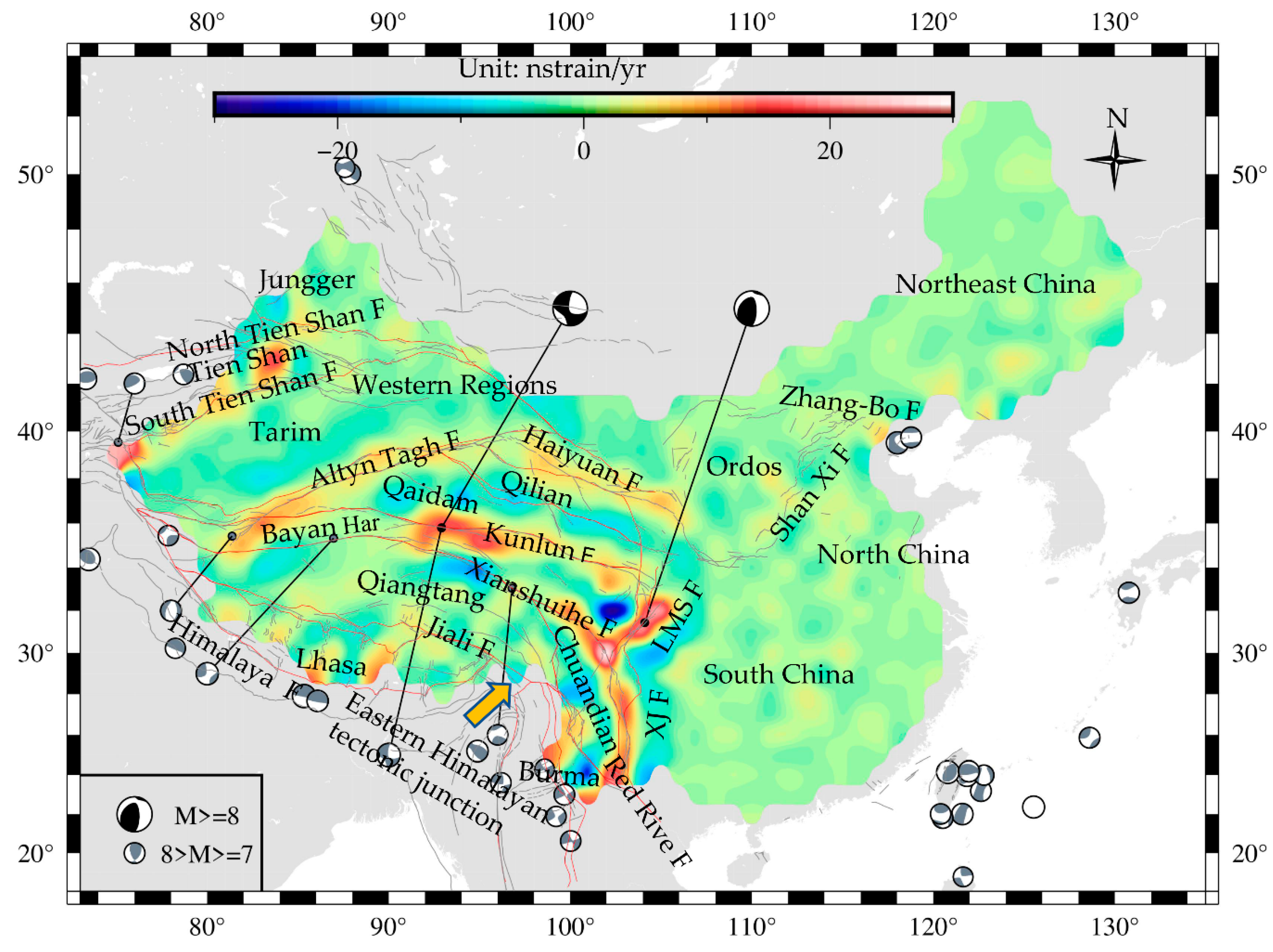
We record the distribution of earthquakes of magnitude 7 and above 7 from January 1963 to September 2020 (Figure 7) (seismic data from https://www.globalcmt.org/CMTsearch.html). The frequency of earthquakes is relatively high and earthquakes above magnitude 8 are all located in western China. However, earthquake above magnitude 7 (including magnitude 7) occurs twice only in eastern China. The distribution of earthquakes in continental China is obviously strong in the west and weak in the east. Strong earthquakes mainly occur near active faults, active blocks, and boundary zones of blocks.
We find from Figure 7 that the distribution of a strong earthquake and the direction and size of the velocity field has an obvious connection that strong earthquakes occur in places where the size and direction of the velocity field have great changes. For instance, the direction and size of the velocity field from the Tarim block to the Tien Shan block has obvious changes that direction changed from north by west to north by east and the speed is slowly decreased; the size and direction of the velocity field of the Tibetan plateau also have changed significantly that speed of velocity keeps falling down from Himalayan thrust belt in the direction from south to north and from west to east, and the direction of movement changes clockwise from northeast to the south; the velocity decreases from north to south constantly and the direction of the velocity field changes from east to southeast to the south in Sichuan-Yunnan region.
The type of earthquake is closely related to the strain rate. The distribution of strain rate on the edge of Tibetan Plateau is mainly compression and there is a strong crustal shortening in the Himalayan thrust nappe belt and Qilian mountain area, which caused the Tibetan plateau area earthquake for thrust earthquakes. And the inner of plateau mainly shows tension effect and strike-slip effect, which results in that majority of an inner strong earthquake in the Tibetan Plateau are normal faults and strike-slip fault type earthquake.
We find that the distribution of a strong earthquake and the second strain rate invariant have an obvious connection that all the earthquakes distribute in the area where the second strain rate invariant is greater than 20 nstrain/yr from Figure 7. There have been two strong earthquakes in the Tangshan area where the second strain rate invariants are about 20~25 nstrain/yr. Besides, it could be found that the Tien Shan Mountain, Tibetan Plateau, and Sichuan-Yunnan region are the regions where the second strain rate invariant is large, and the second strain rate invariant varies greatly. The second strain rate invariant range of Tien Shan region, Tibetan Plateau, Sichuan-Yunnan are about 5~45, 8~68, 12~46 nstrain/yr respectively. Actually, the strong earthquakes widely take place in the Tibetan Plateau, Sichuan-Yunnan, and Tien Shan region, and strong earthquake activities in other areas are relatively weak. Therefore, we conduct that the occurrence of strong earthquakes is closely related to the magnitude and rate of change of the second strain rate invariant.
To further explore the relationship between areas with a high incidence of strong earthquakes and spatial change of strain rate, the variation of the second strain rate invariant is treated by neighborhood point difference. Subtract the second strain invariant of each grid from the second strain rate invariant of its surrounding adjacent grid. Take the average of the adjacent different values. We obtain a distribution of the neighborhood differences of the second strain rate invariant (Figure 8).
It can be seen from Figure 8 that the fault zone exists in the area where the neighborhood difference of the second strain rate invariant is large. For instance, the Altyn Tagh fault zone, Haiyuan fault zone, the North Tien Shan fault zone, the Kunlun fault zone, the Xiaojiang fault zone, the Red River fault zone and the Shan Xi fault zone, and the Zhang-Bo fault zone are all located in the area with high difference value in Figure 8. The strong earthquake is mainly along the vast fault zone which often constitutes a block boundary [47]. This shows that the fault area has a large strain difference, which affects the occurrence of earthquakes.
Epicenter location of the earthquake of magnitude 8 and above 8 magnitude overlap with the position of the maximum of the second strain rate invariants neighborhood difference. The epicenter location of earthquakes magnitude 8 and above are all in the red and white area, where the second strain rate invariants neighborhood difference is about 15~28 nstrain/yr. The epicenter location of earthquakes magnitude 7 and above distribute in the yellow and red areas in Figure 8. The second strain rate invariants neighborhood difference is about 5~25 nstrain/yr. Therefore, a strong earthquake occurred in the area where the second strain rate invariants neighborhood difference is large.
It illustrates that the larger the second strain rate invariants neighborhood difference is, the higher the magnitude of the earthquake will be. The larger the neighborhood difference of the second strain rate invariant is, the higher the frequency of strong earthquakes is. The second strain rate invariant characterizes the energy characteristics of regional crustal deformation, which means that strong earthquakes are closely related to the energy difference.
According to the above areas with a high occurrence of strong earthquakes, we have summarized some laws. At first, strong earthquakes occur in places where the size and direction of the velocity field have great changes. The change of velocity field is caused by the tectonic difference of different active blocks. The greater the velocity change in blocks, the higher the frequency of strong earthquakes is. Secondly, strong earthquakes tend to occur in regions with large strain rate and strain rate variation. All earthquakes of magnitude 7 and above are distributed in regions where the second strain rate invariant is more than 20 nstrain/yr. The non-uniform distribution of strain rate and the accumulation of large strain is the internal reasons for the occurrence of strong earthquakes. Finally, strong earthquakes occur in areas with large neighborhood differences of the second strain rate invariant, which indicates that the larger the neighborhood differences of the second strain rate invariant are, the stronger the magnitude of earthquakes will be, and the higher the frequency of strong earthquakes will be. The second strain rate invariant characterizes the energy characteristics of regional crustal deformation, which means that strong earthquakes are closely related to the energy accumulation difference in space.
5. Conclusions
We used the interpolation method of two-dimensional vector velocity field data based on Green’s function to conduct coupled interpolation with a Poisson’s ratio of 0.5 for 1966 horizontal velocity field data of GNSS stations from 1999 to 2017 and obtained the uniform velocity field and strain rate field with a grid of 1°. In this study, the direct verification method and the cross-validation method were used for error analysis, and the error of interpolation is small. The error results show that the reliability of the model is good.
Based on the results of velocity field interpolation and strain rate, the spatial distribution of the measured velocity field of the horizontal crustal movement in continental China is uneven and has obvious zoning characteristics. The velocity field numerical value in the west is large, while the velocity field numerical value in the east is small. On the other hand, from the aspect of motion direction analysis, the west part of China has a consistent north-northeast movement, while the east part of China has a consistent south-southeast movement. Except for the active block in Northeast Asia, the overall trend of velocity field motion direction moves clockwise from west to east. Besides, the maximum shear strain rate values in the eastern part of China are very small, and the overall crustal shear deformation is feeble. On the contrary, the western part of continental China shows a large maximum shear strain rate.
Research finds that the maximum shear strain rate and the second strain rate invariant is relatively similar. It presents that with the eastern Himalayan structure as the center, the eastern Lhasa block, the eastern Qiangtang block, the Sichuan-Yunnan block, and the Burma block form a strong deformation rate zone of continuous deformation in the fan-shaped region, which has been a strong deformation rate zone for earthquakes of magnitude 7 or higher in continental China since 1963.
As the results of tectonic interpretation, the distribution of concentrated shear strain rate distribution Kunlun fault zone and Xianshuihe fault zone shows that the eastward movement of regional crustal material on either side of the main fault zone is different, and the speed of material movement in the south fault zone is higher than in the north zone. The strong shear deformation in the Sichuan-Yunnan block, the Bayan Har block, the Lhasa block, and the Qiangtang block is the result of the lateral (east and west) movement of crustal material in the Tibetan Plateau. The shear strain rate field of the Xiaojiang fault zone and the Longmen Shan fault zone shows that the eastward movement of crustal material in Tibetan Plateau is blocked by the stable South China block. Therefore, the direction of crustal material movement is deflected, and a clockwise rotation motion system centered on the eastern Himalayan structure is gradually formed. The strong rotation rate and weak shear strain rate distribution in the eastern Himalayan tectonic junction indicates that the region is characterized by continuous and unified crustal vortex movement.
The crustal shortening zone is mainly concentrated in the thrust zone of the Himalayan main boundary, Qilian block with its boundary and South Tien Shan fault zone along the boundary between the Tarim block and the Tien Shan block. Besides, Crustal expansion belt mainly concentrated in the Qiangtang block, inside of the Bayan Har block, and the western boundary of the Sichuan-Yunnan block. There is a 10~30 nstrain/yr arc expansion band between the JiaLi fault and the Xianshuihe fault. It goes from the southwest of Lhasa to Qamdo, coming through Lijiang, finally to the bottom of the south of the Burma block.
According to the results of earthquake analysis, the high incidence of strong earthquakes in China is located in The Tien Shan, Tibetan Plateau, and Sichuan-Yunnan regions. The influencing factors of strong earthquakes include velocity change, non-uniform strain distribution, accumulation of larger strain and the difference of the second strain rate invariant. The greater the velocity variation in the active block area, the higher the frequency of strong earthquakes. The non-uniform distribution of strain rate and the accumulation of larger strain are the internal causes of strong earthquakes. Strong earthquakes are closely related to the difference in energy accumulation in space.
Author Contributions
W.B. and J.W. conceived and designed the experiments; W.W. processed the CMONOC data; W.B. wrote the main manuscript text; J.W. helped with the writing of the text. All authors have read and agreed to the published version of the manuscript.
Funding
This work is supported by the Natural Science Foundation of China (Grant Nos. 41674003, and 41874004).
Acknowledgments
The CMONOC data were downloaded from the Institute of Earthquake Science, China Earthquake Administration. Some of the Figures were prepared using the GMT graphics package (Wessel and Smith, 1991).
Conflicts of Interest
The authors declare no conflict of interest.
References
- Zhang, P.Z.; Zhang, G. Academic progress on the mechanism and forecast for continental strong earthquake in the first two years. China Basic Sci. 2000, 10, 4–10. [Google Scholar]
- Rong, Y.; Xu, X.; Shen, Z.-K. A probabilistic seismic hazard model for Mainland China. Earthquake Spectra. Earthq. Spectra 2020, 36 (Suppl. 1), 181–209. [Google Scholar] [CrossRef]
- Wang, M.; Shen, Z.K. Present day crustal deformation of continental China derived from GPS and its tectonic implications. J. Geophys. Res. Solid Earth 2020, 125, 1–22. [Google Scholar] [CrossRef] [Green Version]
- Shen, Z.K.; Wang, M. Crustal deformation along the Altyn Tagh fault system, western China, from GPS. J. Geophys. Res. Solid Earth 2001, 106, 30607–30621. [Google Scholar] [CrossRef]
- Wang, Q.; Zhang, P.Z. Present-Day Crustal Deformation in China Constrained by Global Positioning System Measurements. Science 2001, 294, 574–577. [Google Scholar] [CrossRef] [Green Version]
- Yang, S.M.; Li, J. The present deformation and fault activity of Tianshan Mountain were studied by GPS. Sci. China 2008, 38, 872–880. [Google Scholar]
- Gan, W.; Shen, Z.K. Horizontal crustal movement of Tibetan Plateau from GPS measurements. J. Geod. Geodyn. 2004, 24, 29–35. [Google Scholar]
- Burchfiel, B.C.; Brown, E.T. Crustal Shortening on the Margins of the Tien Shan, Xinjiang, China. Int. Geol. Rev. 2010, 41, 665–700. [Google Scholar] [CrossRef]
- Holt, W.E.; Haines, A.J. Velocity field in Asia inferred from Quaternary fault slip rates and Global Positioning System observations. J. Geophys. Res. Solid Earth 2000, 105, 19185–19209. [Google Scholar] [CrossRef]
- Bendick, R.; Freymueller, J. Geodetic evidence for a low slip rate in the Altyn Tagh fault system. Nature 2000, 404, 69–72. [Google Scholar] [CrossRef]
- Wang, W.; Qiao, X.; Yang, S. Present-day velocity field and block kinematics of Tibetan Plateau from GPS measurements. Geophys. J. Int. 2017, 208, 1088–1102. [Google Scholar] [CrossRef]
- Thatcher, W.; Savage, J.C.; Simpson, R.W. The Eastern California Shear Zone as the northward extension of the southern San Andreas Fault. J. Geophys. Res. Solid Earth 2016, 121, 2904–2914. [Google Scholar] [CrossRef] [Green Version]
- Loveless, J.P.; Meade, B.J. Partitioning of localized and diffuse deformation in the Tibetan Plateau from joint inversions of geologic and geodetic observations. Earth Planet. Sci. Lett. 2011, 303, 11–24. [Google Scholar] [CrossRef] [Green Version]
- England, P.; Molnar, P. Right-lateral shear and rotation as the explanation for strike-slip faulting in eastern Tibet. Nature 1990, 344, 140–142. [Google Scholar] [CrossRef]
- Deng, Q.D.; Zhang, P.Z. Basic characteristics of active tectonics of China. Sci. China 2003, 46, 356–371. [Google Scholar]
- Arnoso, J.; Riccardi, U. Strain Pattern and Kinematics of the Canary Islands from GNSS Time Series Analysis. Remote Sens. 2020, 12, 3297. [Google Scholar] [CrossRef]
- Chen, B.; Dai, W.J. Reconstruction of Wet Refractivity Field Using an Improved Parameterized Tropospheric Tomographic Technique. Remote Sens. 2020, 12, 3034. [Google Scholar] [CrossRef]
- He, X.; Yu, K.G. GNSS-TS-NRS: An Open-Source MATLAB-Based GNSS Time Series Noise Reduction Software. Remote Sens. 2020, 12, 3532. [Google Scholar] [CrossRef]
- Tavani, S.; Pignalosa, A. Photogrammetric 3D Model via Smartphone GNSS Sensor: Workflow, Error Estimate, and Best Practices. Remote Sens. 2020, 12, 3616. [Google Scholar] [CrossRef]
- Bilham, R.; Freymueller, J. GPS measurements of present-day convergence across the Nepal Himalaya. Nature 1997, 386, 61–64. [Google Scholar] [CrossRef]
- Jouanne, F.; Mugnier, J.L. Oblique Convergence in the Himalayas of Western Nepal Deduced from Preliminary Results of GPS Measurements. Geophys. Res. Lett. 1999, 26, 1933–1936. [Google Scholar] [CrossRef] [Green Version]
- Shen, Z.K.; Zhao, C.; Yin, A. Contemporary crustal deformation in east Asia constrained by Global Positioning System measurements. J. Geophys. Res. Solid Earth 2000, 105, 5721–5734. [Google Scholar] [CrossRef]
- Paul, J.; Bürgmann, R.; Gaur, V.K. The motion and active deformation of India. Geophys. Res. Lett. 2001, 28, 647–650. [Google Scholar] [CrossRef] [Green Version]
- Wang, Q.; Zhang, P.Z. Present-day crustal movement and tectonic deformation in China continent. Sci. China 2002, 45, 865–874. [Google Scholar] [CrossRef]
- Zhang, P.Z.; Wang, Q. GPS velocity field and active crustal blocks of contemporary tectonic deformation in continent China. Earth Sci. Front. 2002, 9, 187–198. [Google Scholar]
- Chen, Z.B. Global Positioning System measurements from eastern Tibet and their implications for India/Eurasia intercontinental deformation. J. Geophys. Res. 2000, 105, 16215–16227. [Google Scholar] [CrossRef]
- Gan, W.; Zhang, P.Z.; Shen, Z.K. Present-day crustal motion within the Tibetan Plateau inferred from GPS measurements. J. Geophys. Res. 2007, 112. [Google Scholar] [CrossRef] [Green Version]
- Zheng, G.; Wang, H. Crustal Deformation in the India-Eurasia Collision Zone From 25 Years of GPS Measurements. J. Geophys. Res. Solid Earth 2017, 122, 9290–9312. [Google Scholar] [CrossRef]
- Haines, A.J.; Wallace, L.M. New Zealand-Wide Geodetic Strain Rates Using a Physics-Based Approach. Geophys. Res. Lett. 2020, 47, e2019GL084606. [Google Scholar] [CrossRef]
- Weiss, J.R.; Walters, R.J. High-resolution surface velocities and strain for Anatolia from Sentinel-1 InSAR and GNSS data. Geophys. Res. Lett. 2020, 47, e2020GL087376. [Google Scholar] [CrossRef]
- Kahle, H.G.; Cocard, M.; Peter, Y. GPS-derived strain rate field within the boundary zones of the Eurasian, African, and Arabian Plates. J. Geophys. Res. Solid Earth 2000, 105, 23353–23370. [Google Scholar] [CrossRef]
- Wdowinski, S.; Sudman, Y. Geodetic detection of active faults in S. California. Geophys. Res. Lett. 2001, 28, 2321–2324. [Google Scholar] [CrossRef] [Green Version]
- Allmendinger, R. Strain and rotation rate from GPS in Tibet, Anatolia, and the Altiplano. Tectonics 2007, 26. [Google Scholar] [CrossRef] [Green Version]
- Shen, Z.K.; Wang, M. Optimal Interpolation of Spatially Discretized Geodetic Data. Bull. Seismol. Soc. Am. 2015, 105, 2117–2127. [Google Scholar] [CrossRef] [Green Version]
- Wessel, P.; Luis, J.F. The Generic Mapping Tools Version 6. Geochem. Geophys. Geosyst. 2019, 20, 5556–5564. [Google Scholar] [CrossRef] [Green Version]
- Melachroinos, S.A.; Lemoine, J.M.; Tregoning, P.; Biancale, R. Quantifying FES2004 S2 tidal model from multiple space-geodesy techniques, GPS and GRACE, over North West Australia. J. Geod. 2009, 83, 915–923. [Google Scholar] [CrossRef]
- Ponte, R.M.; Ray, R.D. Atmospheric pressure corrections in geodesy and oceanography: A strategy for handling air tides. Geophys. Res. Lett. 2002, 29, 61–64. [Google Scholar] [CrossRef]
- Schmid, R.; Dach, R.; Collilieux, X.; Jäggi, A.; Schmitz, M.; Dilssner, F. Absolute IGS antenna phase center model igs08.atx: Status and potential improvements. J. Geodesy 2016, 90, 343–364. [Google Scholar] [CrossRef] [Green Version]
- Wu, W.W. A High-Precision GPS Data Processing and Contemporary Crustal Deformation in China Mainland. Ph.D. Thesis, Tongji University, Shanghai, China, 2018. [Google Scholar]
- Wu, W.W.; Wu, J.C. A Study of Rank Defect and Network Effect in Processing the CMONOC Network on Bernese. Remote Sens. 2018, 10, 357. [Google Scholar] [CrossRef] [Green Version]
- Sandwell, D.T.; Wessel, P. Interpolation of 2-D vector data using constraints from elasticity. Geophys. Res. Lett. 2016, 43, 10703–10709. [Google Scholar] [CrossRef]
- Hackl, M.; Malservisi, R. Strain rate patterns from dense GPS networks. Nat. Hazards Earth Syst. Sci. 2009, 9, 1177–1187. [Google Scholar] [CrossRef] [Green Version]
- Savage, J.C.; Gan, W. Strain accumulation and rotation in the Eastern California Shear Zone. J. Geophys. Res. Solid Earth 2001, 106, 21995–22007. [Google Scholar] [CrossRef]
- Wdowinski, S.; Smith-Konter, B.; Bock, Y.; Sandwell, D. Diffuse interseismic deformation across the Pacific–North America plate boundary. Geology 2007, 35, 311–314. [Google Scholar] [CrossRef]
- Shen, Z.K.; Lü, J.; Wang, M.; Bürgmann, R. Contemporary crustal deformation around the southeast borderland of the Tibetan Plateau. J. Geophys. Res. Solid Earth 2005, 110. [Google Scholar] [CrossRef] [Green Version]
- Zhang, P.Z.; Deng, Q.D. Strong earthquake activities and active blocks in continental China. Sci. China 2003, 33, 12–20. [Google Scholar]
- Zhang, P.Z.; Deng, Q.D. Active faults, earthquake hazards and associated geodynamic processes in continental China. Scie. Sin. Terra 2013, 43, 1607–1616. (In Chinese) [Google Scholar]
Figure 1.
The distribution of earthquake in China. Black arrows indicate motion directions of the Indian plate and continental China. (the earthquake data from https://www.globalcmt.org/CMTsearch.html).
Figure 1.
The distribution of earthquake in China. Black arrows indicate motion directions of the Indian plate and continental China. (the earthquake data from https://www.globalcmt.org/CMTsearch.html).

Figure 2.
Interpolating horizontal velocity field in continental China (the red lines represent original velocity field data, and the blue lines represent interpolating velocity field data).
Figure 2.
Interpolating horizontal velocity field in continental China (the red lines represent original velocity field data, and the blue lines represent interpolating velocity field data).

Figure 3.
The horizontal strain rate distribution field in continental China. The black line is the boundary line of the first active block; The red line is part of the boundary line of the second active block; Chuandian represents Sichuan-Yunnan.
Figure 3.
The horizontal strain rate distribution field in continental China. The black line is the boundary line of the first active block; The red line is part of the boundary line of the second active block; Chuandian represents Sichuan-Yunnan.

Figure 4.
Continuum deformation field of continental China derived from interpolation of velocities (the black line is the boundary line of the first active block; the red line is part of the boundary line of the second active block; the gray lines represent the fault; Chuandian represents Sichuan-Yunnan; XJ F represents Xiaojiang fault; LMS F represents Longmen Shan fault):(a) The maximum shear strain rate; (b) The dilation rate; (c) The second strain rate invariant; (d) The rotation rate(Assume that the clockwise rotation is positive).

Figure 5.
Direct validation and cross-validation of velocity residual results: (a) The easterly velocity residual of direct verification; (b) The northerly velocity residual of direct verification; (c) The easterly velocity residual of cross-verification; (d) The easterly velocity residual of cross-verification.


Figure 6.
Block motion model. Blue arrows indicate motion directions. Red fan shapes denote block rotation rates. The thick black line is the boundary line of the first active block; The red line is part of the boundary line of the second active block; Chuandian represents Sichuan-Yunnan; XJ F represents Xiaojiang fault; LMS F represents Longmen Shan fault.

Figure 7.
The distribution of strong earthquake and the second strain rate invariant is shown in background-color. Chuandian represents Sichuan-Yunnan.
Figure 7.
The distribution of strong earthquake and the second strain rate invariant is shown in background-color. Chuandian represents Sichuan-Yunnan.

Figure 8.
The neighborhood differences of the second strain rate invariant (the red line is part of the boundary line of the second active block; the gray lines represent the fault; Chuandian represents Sichuan-Yunnan; XJ F represents Xiaojiang fault, LMS F represents Longmen Shan fault).
Figure 8.
The neighborhood differences of the second strain rate invariant (the red line is part of the boundary line of the second active block; the gray lines represent the fault; Chuandian represents Sichuan-Yunnan; XJ F represents Xiaojiang fault, LMS F represents Longmen Shan fault).


Table 1.
The information on GNSS networks.
| Name of the GNSS Network | Number of Continuous Stations | Number of Staging Stations | Time Span | Organization |
|---|---|---|---|---|
| Crustal Movement Observation Network of China (CMONOC) I | 27 | 1079 | 1999~2017 | CMONOC I |
| CMONOC II | 240 | 1078 | 2010~2018 | CMONOC II |
| Red river Fault Zone Monitoring Network | 4 | 12 | 2014~2018 | Tongji University, China |
| Himalaya South Foot Monitoring Network | 34 | 0 | 2004~2016 | California Institute of Technology, USA |
| Zhang-Bo Fault Zone Monitoring Network | 14 | 11 | 2007~2013 | Institute of Earthquake Forecasting, CEA |
| Liupanshan Fault Zone Monitoring Network | 10 | 0 | 2013~2016 | Institute of Earthquake Forecasting, CEA |
| West Sichuan Net | 0 | 95 | 2010~2016 | Institute of Earthquake Forecasting, CEA |
| International Terrestrial Reference Frame (ITFR) 2014 Network | 161 | 0 | 1999~2017 | International Earth Rotation Service |
Table 2.
The range and mean value of the strain rate index of first-grade blocks in continental China.
Table 2.
The range and mean value of the strain rate index of first-grade blocks in continental China.
| Northeast Asia | North China | South China | Burma | Tibetan | Western Regions | |
|---|---|---|---|---|---|---|
| The range of (nstrain/yr) | −1.35~9.10 | −2.46~8.61 | −2.47~13.75 | 11.55~36.22 | −0.70~45.20 | −6.21~28.05 |
| The mean of (nstrain/yr) | 2.26 | 2.65 | 1.62 | 24.91 | 18.22 | 3.64 |
| The range of (nstrain/yr) | −10.71~2.29 | −10.11~1.22 | −46.65~2.26 | −27.82~−1.53 | −53.090~4.53 | −41.47~0.24 |
| The mean of (nstrain/yr) | −2.42 | −3.00 | −3.83 | −17.12 | −17.56 | −9.16 |
| The range of (nstrain/yr) | 0.21~7.18 | 0.29~7.34 | 0.26~25.86 | 6.54~32.02 | 1.04~47.68 | 0.50~34.75 |
| The mean of (nstrain/yr) | 2.34 | 2.82 | 2.72 | 21.01 | 17.89 | 6.40 |
| The range of (nstrain/yr) | −7.91~7.8 | −8.26~8.74 | −41.57~6.25 | −2.90~15.65 | −38.84~28.80 | −31.78~7.38 |
| The mean of (nstrain/yr) | −0.16 | −0.35 | −2.21 | 7.78 | 0.65 | −5.53 |
| The range of (nstrain/yr) | −7.12~4.93 | −7.41~4.77 | −15.88~6.02 | −16.75~22.00 | −41.77~42.47 | −11.76~17.11 |
| The mean of (nstrain/yr) | −1.29 | −1.08 | −0.55 | 7.19 | 0.54 | 2.88 |
| The range of (nstrain/yr) | 0.50~11.06 | 0.49~10.39 | 0.55~46.92 | 11.65~45.67 | 8.03~67.86 | 0.82~50.06 |
| The mean of (nstrain/yr) | 3.77 | 4.58 | 4.72 | 30.85 | 26.32 | 10.59 |
Table 3.
Direct verification and cross-verification of speed error results.
| Error | ME 1 | MAE 1 | RMSE 1 | ME 2 | MAE 2 | RMSE 2 |
|---|---|---|---|---|---|---|
| The easterly velocity (mm/yr) | 1.08 × 10⁻⁶ | 0.4590 | 0.7679 | −0.0148 | 0.5526 | 0.7128 |
| The northerly velocity (mm/yr) | −4.19 × 10⁻⁶ | 0.4558 | 0.7874 | −0.0565 | 0.6281 | 0.8088 |
1 error parameters for direct validation, 2 error parameters for cross-validation.
Publisher’s Note: MDPI stays neutral with regard to jurisdictional claims in published maps and institutional affiliations. |
© 2020 by the authors. Licensee MDPI, Basel, Switzerland. This article is an open access article distributed under the terms and conditions of the Creative Commons Attribution (CC BY) license (http://creativecommons.org/licenses/by/4.0/).
Share and Cite
MDPI and ACS Style
Bian, W.; Wu, J.; Wu, W. Recent Crustal Deformation Based on Interpolation of GNSS Velocity in Continental China. Remote Sens. 2020, 12, 3753. https://0-doi-org.brum.beds.ac.uk/10.3390/rs12223753
AMA Style
Bian W, Wu J, Wu W. Recent Crustal Deformation Based on Interpolation of GNSS Velocity in Continental China. Remote Sensing. 2020; 12(22):3753. https://0-doi-org.brum.beds.ac.uk/10.3390/rs12223753
Chicago/Turabian StyleBian, Weiwei, Jicang Wu, and Weiwei Wu. 2020. "Recent Crustal Deformation Based on Interpolation of GNSS Velocity in Continental China" Remote Sensing 12, no. 22: 3753. https://0-doi-org.brum.beds.ac.uk/10.3390/rs12223753
Note that from the first issue of 2016, this journal uses article numbers instead of page numbers. See further details here.