Springtime Upwelling and Its Formation Mechanism in Coastal Waters of Manaung Island, Myanmar

1
Third Institute of Oceanography, Ministry of Natural Resources, Xiamen 361005, China
2
Southern Marine Science and Engineering Guangdong Laboratory (Zhuhai), Zhuhai 519082, China
3
Laboratory for Regional Oceanography and Numerical Modeling, Qingdao National Laboratory for Marine Science and Technology, Qingdao 266237, China
4
State Key Laboratory of Marine Environmental Science, College of Ocean and Earth Sciences, Xiamen University, Xiamen 361102, China
5
Marine Science Department, Pathein University, Pathein 10014, Myanmar
*
Author to whom correspondence should be addressed.
Remote Sens. 2020, 12(22), 3777; https://0-doi-org.brum.beds.ac.uk/10.3390/rs12223777
Submission received: 30 September 2020
/
Revised: 14 November 2020
/
Accepted: 16 November 2020
/
Published: 18 November 2020
(This article belongs to the Special Issue Remote Sensing Applications in Ocean Observation)
Abstract
:Multisource satellite remote sensing data and the World Ocean Atlas 2018 (WOA18) temperature and salinity dataset have been used to analyze the spatial distribution, variability and possible forcing mechanisms of the upwelling off Manaung Island, Myanmar. Signals of upwelling exist off the coasts of Manaung Island, in western Myanmar during spring. It appears in February, reaches its peak in March and decays in May. Low-temperature (<28.3 °C) and high-salinity (>31.8 psu) water at the surface of this upwelling zone is caused by the upwelling of seawater from a depth below 100 m. The impact of the upwelling on temperature is more significant in the subsurface layer than that in the surface layer. In contrast, the impact of the upwelling on salinity in the surface layer is more significant. Further research reveals that the remote forcing from the equator predominantly induces the evolution of the upwelling, while the local wind forcing also contributes to strengthen the intensity of the upwelling during spring.
1. Introduction
Upwelling usually refers to the upward movement of water, caused by the divergence of the flow in the surface layer of the ocean [1]. Since deeper water is usually enriched with nutrients, it tends to increase a supply of nutrients to upper oceanic layers and forms the basis for the high productivity of upwelling regions. Consequently, upwelling areas are among the most fertile regions of the global ocean [2]. The production and its variability over this coastal upwelling system are a key concern for the fishing community, since they may affect the day-to-day livelihood of the coastal population and are important for the Indian Ocean rim countries due to their developing country status [3]. Moreover, upwelling is also an important factor modulating regional and global climate. For example, the upwelling along the western coast of Java-Sumatra has changed sea surface temperature (SST) of the warm pool in the eastern Indian Ocean and caused anomalous atmospheric circulation, thereby affecting intraseasonal to decadal variabilities of the tropical climates [4,5,6,7,8,9]. Therefore, the understanding physical processes and their variabilities in the upwelling systems is important because it gives us crucial information regarding variability of a marine ecosystem and its regional climate [10,11].
The Bay of Bengal (BOB) is dominated by the South Asian monsoon. The southwest monsoon prevails in summer (June–August), while the northeast monsoon prevails in winter (December–February), and the summer monsoon is stronger than the winter monsoon [12]. Upwelling in the BOB mostly occurs in the southwest monsoon period, indicating that it is only a seasonal phenomenon in the Bay [9]. Although the upwelling in the BOB or in the Arabian Sea is mainly driven by the monsoon, the former is much weaker than the latter [13]. This may be principally caused by two factors. Firstly, as a main forcing of the upwelling in either sea areas, the southwest monsoon is much stronger in the Arabian Sea than that in the BOB [14]. Secondly, strong salinity stratification is formed near the surface over the Bay due to abundant rainfall and a large amount of runoff input along its northern coasts [15], which greatly suppresses the intensity of upwelling in the upper layer [16].
In the Indian Ocean, there are four major upwelling systems, including the western Arabian Sea (WAS), the Java and Sumatra coasts (JC), the Seychelles-Chagos thermocline ridge (SCTR) and the Southeastern Bay of Bengal [3]. Many previous works have been done to understand the variabilities of upwelling in WAS, JC and SCTR with timescales ranging from intraseasonal to decadal (e.g., [9,17,18]). In contrast, the existing studies mainly focused on the seasonal variability of the upwelling over the Bay of Bengal due to the sparseness of observational data.
Upwelling in the BOB can be classified into two types. One is coastal upwelling, which mainly occurs along the southern coast of Sri Lanka and the eastern coast of the Indian Peninsula, with relatively fixed locations (Figure 1a). The other is open ocean upwelling generally associated with the activities of cold eddies. The coastal upwelling off southern Sri Lanka occurs during the southwest monsoon, with increased chlorophyll concentrations (>5 mg m−3), and alongshore wind stress is its main cause. In addition, the southwest monsoon, blocked by the island of Sri Lanka, forms a strong positive wind stress curl on the southeastern coast of the island [19]. The upward Ekman pumping induced by the positive curl also makes an important contribution to the development of this upwelling [19,20,21]. The Sri Lanka cold eddy that forms east of Sri Lanka 5–10° N, 83–87° E during the southwest monsoon is induced by the local wind stress with a positive curl [22,23,24].
The strong upwelling around the Madras coast was first reported in 1964 from in-situ data [25], and the upwelled water was found to come from a 30 m layer induced by the strong winds along the coast of Madras. Based on hydrographic data collected during the summer monsoon of 1989, the upwelling zone off the eastern Indian Peninsula (Figure 1a) is found to extend in coastal waters from Madras to Visakhapatnam in summer [26,27], within a range of approximately 40 km offshore. Alongshore winds are an important dynamic mechanism for its formation [15]. Below this upwelling band, downwelling is often observed suggesting the presence of an undercurrent [15].
As mentioned above, previous studies mainly focused on the upwelling in the western boundary of the Bay [19,20,21,22,23,24,25,26,27,28]. In contrast, there are very few reports on the upwelling in its eastern boundary. Yesaki and Jantarapagdee [29] noted wind-induced upwelling over the continental shelf off the west coast of Thailand. The observations of La Fond [30] indicated that during April–May 1963, SST in the northeastern Bay exceeded 28 °C while it was relatively low (<27 °C) in the northern coasts off Myanmar, reflecting the possible impact of cold water upwelling from the subsurface. Follow-up studies also demonstrated the low-temperature zone located at the northwestern coasts of Myanmar 15–20° N during the winter monsoon, which was considered a sign of upwelling [12,31]. This conclusion was also supported by the satellite-derived Chlorophyll-a (Chl-a) data [32]. Akester [33] inferred that the high primary productivity in the continental shelf off Myanmar 16–20° N was caused by the upwelling there in April 2015, and the further evidence of upwelling, including low-temperature, high-salinity and low-dissolved oxygen, was shown in the coastal region.
In summary, although the existing studies have discovered signs of upwelling in the northwestern coasts of Myanmar in winter and spring, most studies were only based on scattered observations from a single cruise. Until now, little has been known about the spatial distribution and seasonal evolution of the upwelling, and there is a lack of research on its dynamic mechanisms. Therefore, in this paper, satellite observations and the World Ocean Atlas 2018 (WOA18) temperature and salinity data were used to analyze the characteristics and causes of the upwelling in the northwestern coast of Myanmar during the winter monsoon. The remainder of this paper is organized as follows: Section 2 introduces the data and method used in this study; Section 3 analyzes the spatial distribution and evolution process of the upwelling in the study area; Section 4 presents the dynamic mechanisms of the upwelling; discussions and, finally, conclusions are stated in Section 5 and Section 6, respectively.
2. Data and Method
2.1. Data
The World Ocean Atlas 2018 (WOA18) has been newly released by the Ocean Climate Laboratory of the National Centers for Environmental Information (NCEI) and the National Oceanic and Atmospheric Administration (NOAA) of the U.S. The WOA18 collected temperature and salinity samples obtained by all ship-deployed Conductivity-Temperature-Depth (CTD) packages, profiling floats, moored and drifting buoys, gliders and undulating oceanographic recorder profiles. Using an objective analysis technique, the raw data are processed into gridded data with a horizontal resolution of 0.25° and 102 vertical levels above 5500 m (including 21 layers, at 5 m spacing, for the top 100 m). Data are presented for climatological composite periods (annual, seasonal, monthly, seasonal and monthly difference fields from the annual mean field, and the number of observations) at 102 standard depths. Standard error of the mean fields is binned into several ranges depending on the depth level. In our study region (90.5–97.5° E, 15.5–21.5° N), the error of temperature in upper 100 m layer ranges from 0.00 to 0.89 °C, and salinity error ranges between 0.00 and 0.33 psu [34,35]. In this study, climatological monthly temperature and salinity were used in the analysis of the upwelling distribution.
The Moderate Resolution Imaging Spectroradiometer (MODIS) daily Chl-a data were provided by the U.S. National Aeronautics and Space Administration (NASA). The chlorophyll concentration was derived using the OC3 algorithm [36]. There is a root mean squared error (RMSE) of 1.228 mg m−3 for MODIS Chl-a against in situ observations [37]. MODIS Chl-a with a horizontal resolution of 4 km [38] spanning between 1 January 2003 and 31 March 2020, were used to study seasonal evolution of the upwelling within the study area.
Sea surface wind data were from the cross-calibrated multi-platform (CCMP) product provided by the NASA’s Physical Oceanography Distributed Active Archive Center (PODAAC). CCMP is a multisource fusion surface wind data derived from satellite observations, including measurements of Special Sensor Microwave Imager (SSM/I), Advanced Microwave Scanning Radiometer for Earth Observing System (AMSR-E) and Tropical Rainfall Measuring Mission Microwave Imager (TMI). To create the CCMP winds, an enhanced variational analysis method (VAM) performs quality control and combines all available Remote Sensing Systems (RSS) cross-calibrated wind data with available conventional ship and buoy data and European Centre for Medium-Range Weather Forecasts (ECMWF) analyses. Overall, the CCMP analysis has the best overall fit to the in-situ observations with an error speed difference ranging from 1.6 m s−1 versus ships to 0.6 m s−1 versus the higher-quality TAO buoys. This is also seen in the RMSE direction fit, which ranges from 11.5° to 7.0°. This dataset has a horizontal resolution of 0.25° × 0.25° and a temporal resolution of 6 h from the period 1993 to 2016 [39].
Daily sea level anomaly (SLA) data were provided by Copernicus Marine Environment Monitoring Service (CMEMS), with a horizontal resolution of 0.25° × 0.25°. This gridded data is derived from the multi-satellite measurements of TOPEX/Poseidon (T/P), European Remote Sensing Satellite-1 (ERS-1) and European Remote Sensing Satellite-2 (ERS-2). There is an error of ~0.02 m for the SLA data [40]. The SLA data we used are from between 1 January 1993 and 31 March 2020. These two data sets of CCMP wind and CMEMS SLA were averaged to obtain weekly and monthly values and then were used to analyze the dynamic mechanisms of the upwelling.
2.2. Method to Identify Area of the Upwelling and Its Intensity
Water that rises to the surface as a result of upwelling is characterized by low-temperature and high-salinity. Both SST and SSS have been extensively used as an indicator of upwelling in many previous studies (e.g., [41,42]). Correspondingly, upwelling areas were identified by a consideration of both SST and SSS from WOA18 in our study. As we shall see below that the region around Myanmar coasts with SST below 28.3 °C has a relatively high salinity. Thus, the regions around the coast of Sri Lanka with SST less than 28.3 °C are used to describe the regions affected by the coastal upwelling.
In addition, the upwelled water from subsurface is typically rich in nutrients. In the upwelling region, surface water has relatively high Chl-a concentration (e.g., [19,41]), besides its typical relatively cold and saline nature. Thus, Chl-a concentration is used as an indicator for the intensity of upwelling in previous works (e.g., [43]). In this study, climatological weekly Chl-a concentration averaged in the upwelling region during January–April is constructed from the daily MODIS Chl-a data and then it is used to explore the evolution processes of the intensity of the upwelling. A larger magnitude of Chl-a concentration denotes a stronger upwelling.
3. Spatial-Temporal Distribution of the Coastal Upwelling off Manaung Island Using WOA18 Data
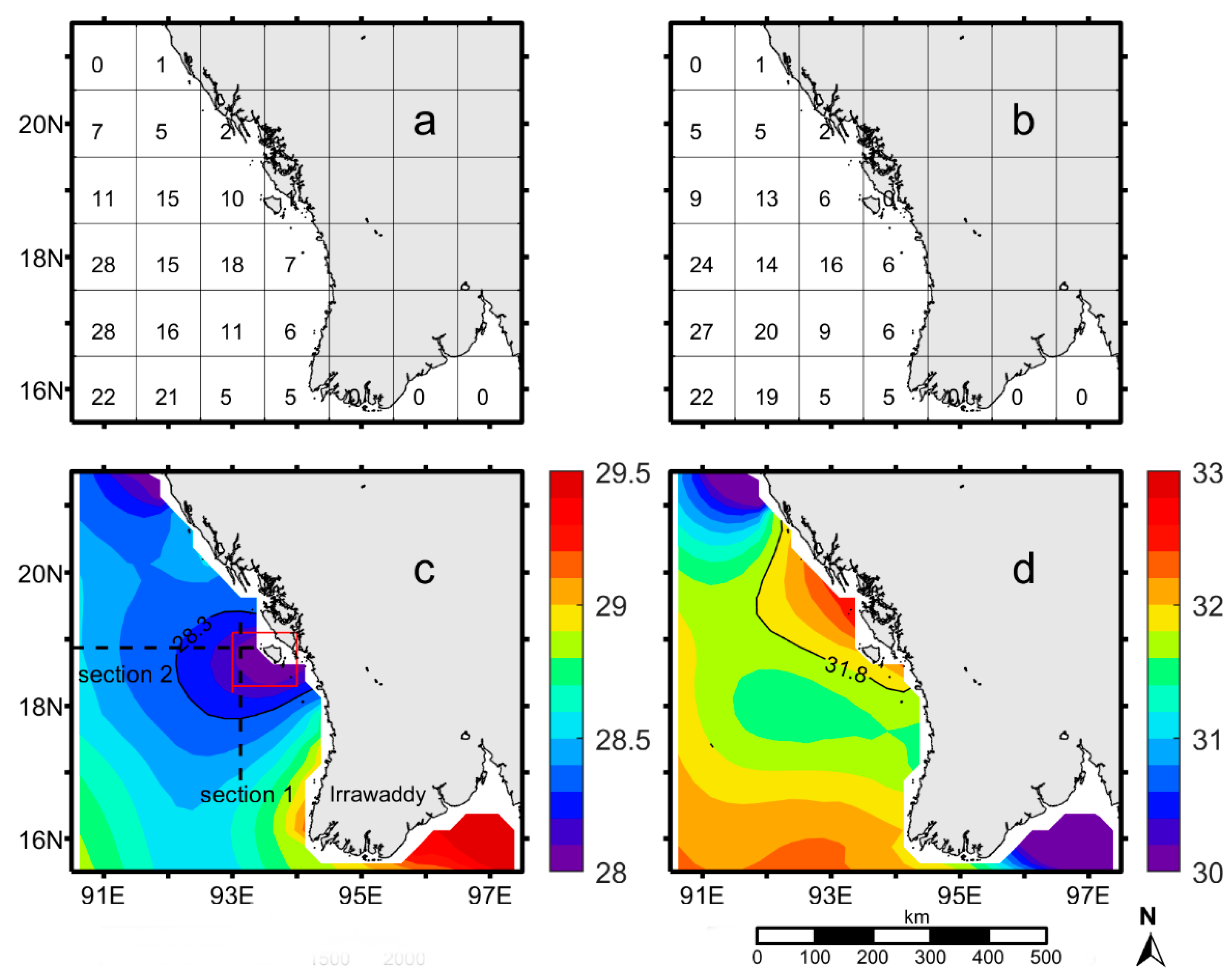
The sample amounts of temperature and salinity in the surface layer for each 1° × 1° grid during spring (March to May) are shown in Figure 2a,b, respectively. Generally speaking, observations of temperature and salinity have a good coverage over the study region. In the coastal areas, the temperature and salinity samples around Manaung Island are 7–18 and 6–16, respectively, and both temperature and salinity samples in open ocean are far larger than that in the nearshore areas. Thus, WOA18 provides adequate data for this study to investigate the spatial structure of the upwelling in the northwestern coasts of Myanmar.
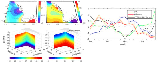
Distributions of surface temperature and salinity in spring are shown in Figure 2c,d, respectively. SST in the study region is relatively high (>28 °C), owing to strong shortwave radiation during spring [44]. The highest SST (29.5 °C) appears in the coastal areas around the estuary of the Irrawaddy River. A low-temperature zone is found distributed along the northwestern coasts of Myanmar, with a cold center located off the coast of Manaung Island. Taken the 28.3 °C isotherm as the boundary of the upwelling, the upwelling zone appears as “tongue-shaped”, extending across 17.7–19.3° N offshore of the Manaung Island, to the east of 92.3° E. Affected by a large amount of runoff and precipitation in the northern Bay, salinity of the study area is relatively low (<33.0 psu). The lowest salinity (~30 psu) occurs offshore of the northwestern Myanmar (Figure 2d). Similar to the low-temperature zone, a high-salinity zone is also formed in the waters around the Manaung Island, with salinity exceeding 31.8 psu, and the high-salinity center is located in the northwestern coast of Manaung Island. The high-salinity (>31.8 psu) and low-temperature (<28.3 °C) zones do not completely overlap, with the high-salinity zone occurring slightly to the north of the low-temperature zone. This low-temperature (<28.3 °C) and high-salinity (>31.8 psu) water at the surface may reflect the occurrence of upwelling near the Manaung Island in spring. This is broadly consistent with the location of upwelling signals revealed by Akester [33] using in-situ data obtained in April 2015.
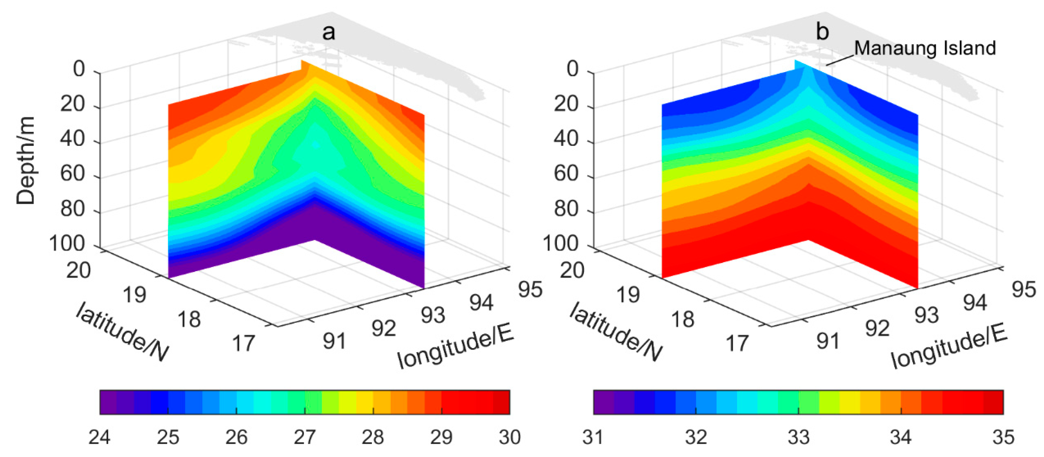
Figure 3 shows the climatologically sectional distributions of temperature and salinity in Section 1 (along 93.375° N) and Section 2 (along 18.875° E) in spring (the locations of the two sections are shown in Figure 2c), illustrating the vertical structure of the upwelling. Both the isotherms and isohalines in the two sections have a trend of rising upwards in the coastal areas of the Manaung Island from about the 100 m layer of the open ocean, indicative of upwelling in the nearshore regions. The remarkable rise of cold subsurface water mainly occurs in coastal waters east of 92° E and north of 17.5° N. The amplitude of the isotherm uplift is significantly smaller in the near-surface layer (above 30 m layer) than that in the subsurface layer (30–70 m). This means that the impact of upwelling on temperature is more pronounced in the subsurface than that in the surface layer. This may be caused by two factors. Firstly, the subsurface layer lies within the seasonal thermocline and the vertical temperature gradient there is larger than that in the near-surface layer, and thus the impact of upwelling on temperature is more significant in the subsurface layer. Secondly, the intensity of upwelling may be partially suppressed by strong salinity stratification in the near-surface layer [16], which further weakens upwelling near the surface and thus results in weaker uplift of isotherm there. The sectional distribution of salinity also reveals upwelling of high-salinity water in the subsurface layer off the coast of Manaung Island (Figure 3b). However, in contrast to temperature, the upwelling of high-salinity water is more significant in the upper layer above 30 m than that in the subsurface layer. This is mainly because both the freshwater input from river discharge and the precipitation into the surface make the vertical salinity gradient larger in the upper layer than that in the subsurface layer [45]. Therefore, even under the condition of a weaker uplift of isotherms in the near-surface layer (Figure 3a), the uplift of isohalines is much more significant in the upper layer.
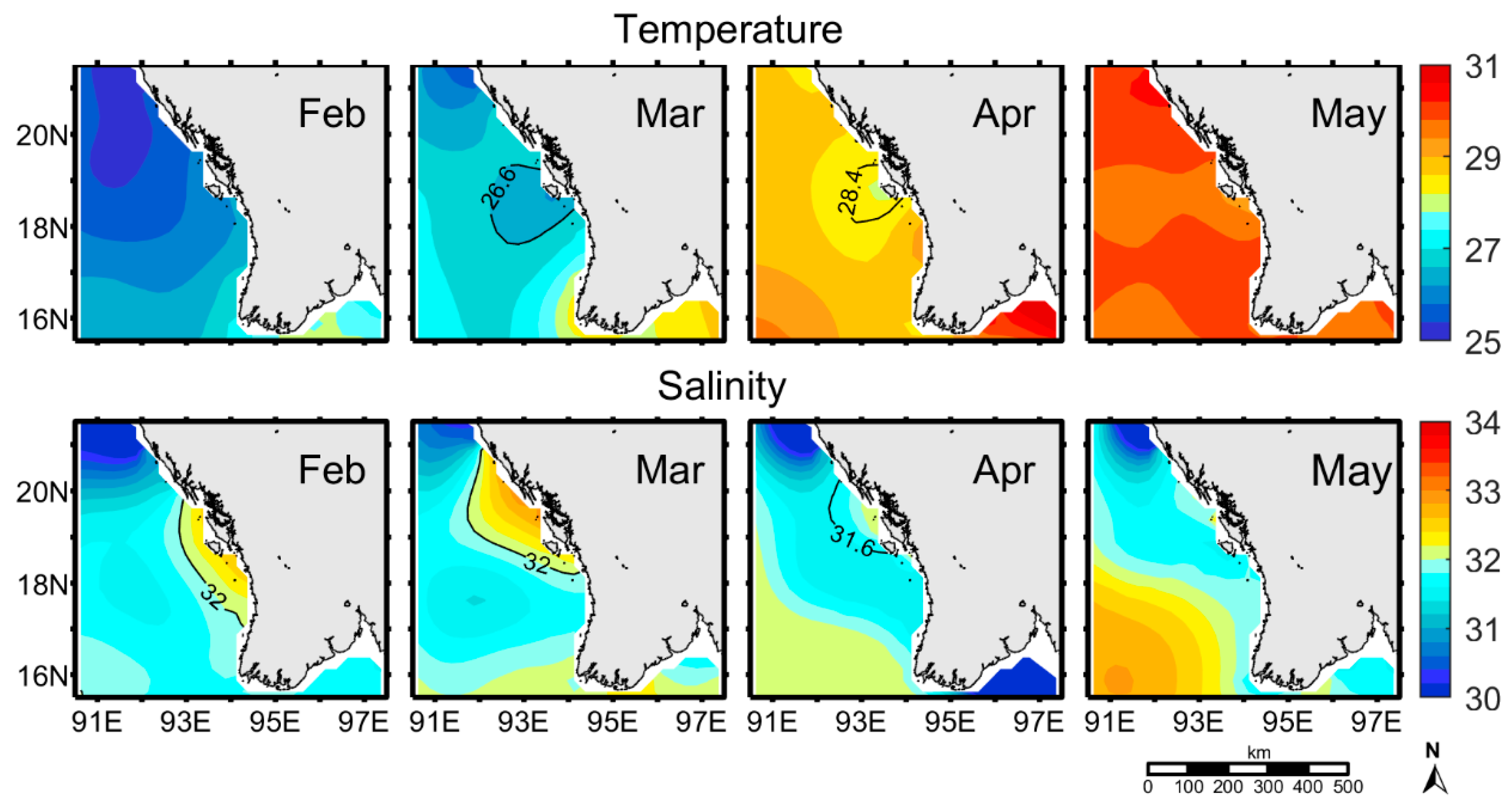
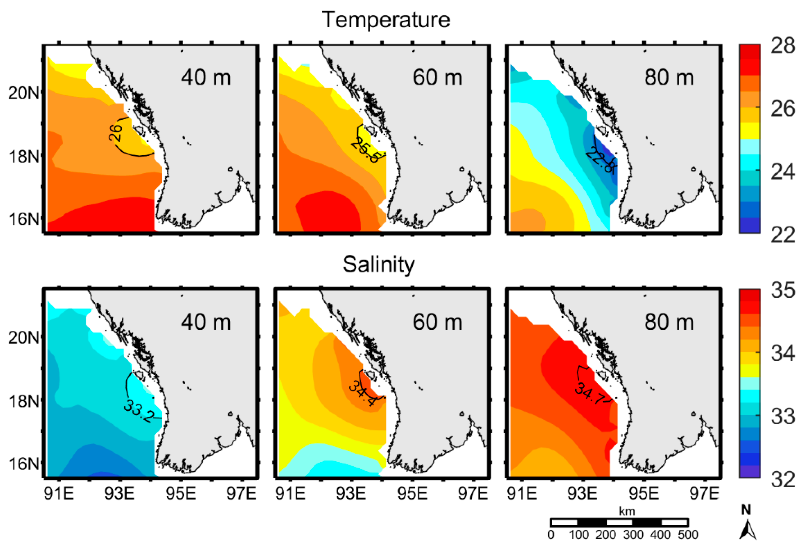
Seasonal evolution for the coastal upwelling off Manaung Island is further explored using WOA18 climatologically monthly temperature and salinity data (Figure 4). In February, a high-salinity zone starts to form in the surface off the coasts of Manaung Island, while the low-temperature signal is not significant. This is mainly because the southward flowing low-temperature water from the northern Bay along the coasts during that period [46] covers the upwelled cold water from subsurface. In fact, both the low-temperature and high-salinity signals of the upwelling are clearly presented in the subsurface layers between 40 and 80 m around the coastal areas of Manaung Island in February (Figure 5). In March, the extent of low-temperature and high-salinity water is the largest, indicating that the coastal upwelling reaches its peak in this month. Subsequently, the extent of low-temperature and high-salinity water significantly shrinks in April and disappears in May. Thus, April and May are periods for the decay and dissipation of the coastal upwelling of Manaung Island.
4. Dynamic Mechanisms for Seasonal Evolution of the Coastal Upwelling of Manaung Island Using Satellite Measurements
As is well known, local surface wind is an important factor influencing the generation and evolution of coastal upwelling [28,47]. Therefore, the role of local wind on the formation and evolution of the coastal upwelling of Manaung Island is explored here.
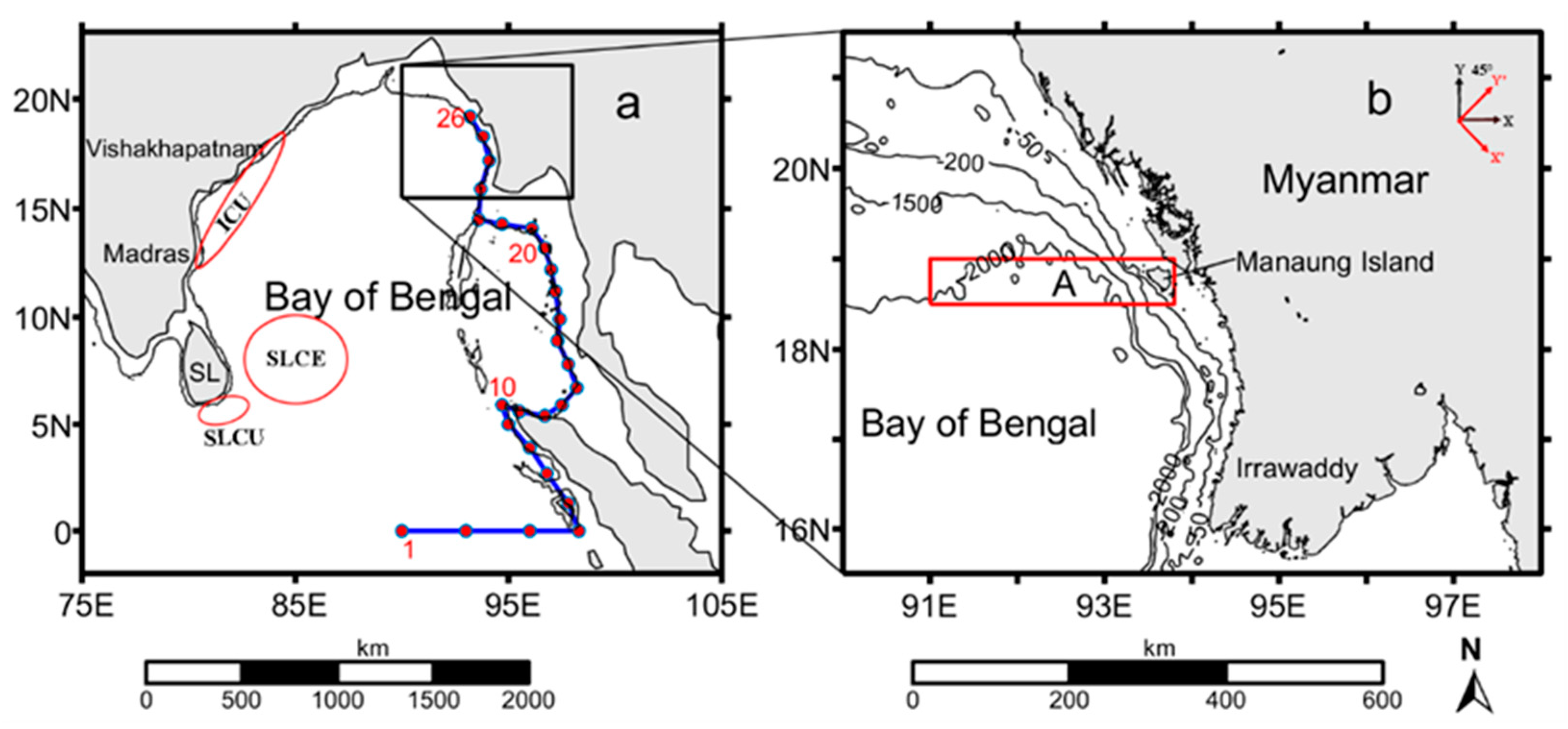
Affected by the South Asian monsoon, the predominant wind in the northern Bay is northwesterly/northerly during winter and spring [12]. The direction of wind stress is roughly parallel to the NW-SE orientation of the coastline of northwestern Myanmar (Figure not shown). According to the classic Ekman transport theory, i.e., in the Northern Hemisphere, the wind blows in a direction parallel to the coast (on the left side of the wind direction), and it causes net movement of surface water at about 90 degrees to the right of the wind direction. Because the surface water flows away from the coast, the water is replaced with water from below [48]. Thus, the northwesterly wind stress will cause an offshore Ekman transport there, thereby triggering the upwelled subsurface water to the surface layer as a compensatory for the offshore transport, which induces the formation of coastal upwelling. To facilitate further analysis, the coordinate axes are rotated clockwise by 45°, and the wind stress is decomposed into directions parallel to and perpendicular to the coasts, with the southeast direction along the coastline being positive (as shown in Figure 1b). During the northeast monsoon (December to April of the following year), the coast of Manaung Island experiences the northwesterly wind, favorable to the formation of upwelling. The wind stress is generally weak (0.01–0.02 N m−2) and reaches its maximum (approximately 0.02 N m−2) in January (Figure 6a). At the same time, the wind stress curl reaches the maximum (approximately 2 × 10⁻⁷ N m−3) (Figure 6b). Then, the wind direction reverses to a southeasterly one during the monsoon transition period in May, which is not favorable to the formation of upwelling. Thus, local wind stress may contribute to the formation of the upwelling in spring, although its intensity is relatively weak, and the timing of its maximum is two months out of phase with the peak of upwelling (in March). That is to say that although the local wind stress contributes to the development of upwelling, there may be other factors (i.e., remote forcing from the equator) that have important contributions to the development of the coastal upwelling of Manaung Island, as we shall see below.
Besides local wind, remote forcing from the equator is also the main forcing that induces seasonal variabilities of the BOB. In particular, it plays a dominant role at the eastern and northern boundary of the Bay [49,50,51]. It affects the interior Bay via the planetary waves (including coastal Kelvin waves and the westward propagating Rossby waves triggered by the equatorial processes) [52]. Referring to Cheng et al. [51], the propagation path of the planetary waves from the equator to the interior Bay along the 200 m isobath (the blue line in Figure 1a) is selected, and the SLA evolutions at each station of December and May of the following year are illustrated (Figure 6c). The upwelling Kelvin wave originates from the equator, propagates into the eastern boundary of the BOB in early February and reaches the coastal region of Manaung Island in early March, resulting in a remarkable decrease in SLA there (Figure 6c). This further amplifies the upwelling induced by the local wind stress (Figure 6a,b), so that the upwelling peaks in March. Subsequently, the downwelling Kelvin wave, triggered by equatorial westerlies in early April, reaches the Manaung Island in early May, thereby making an important contribution to the decay of the upwelling.
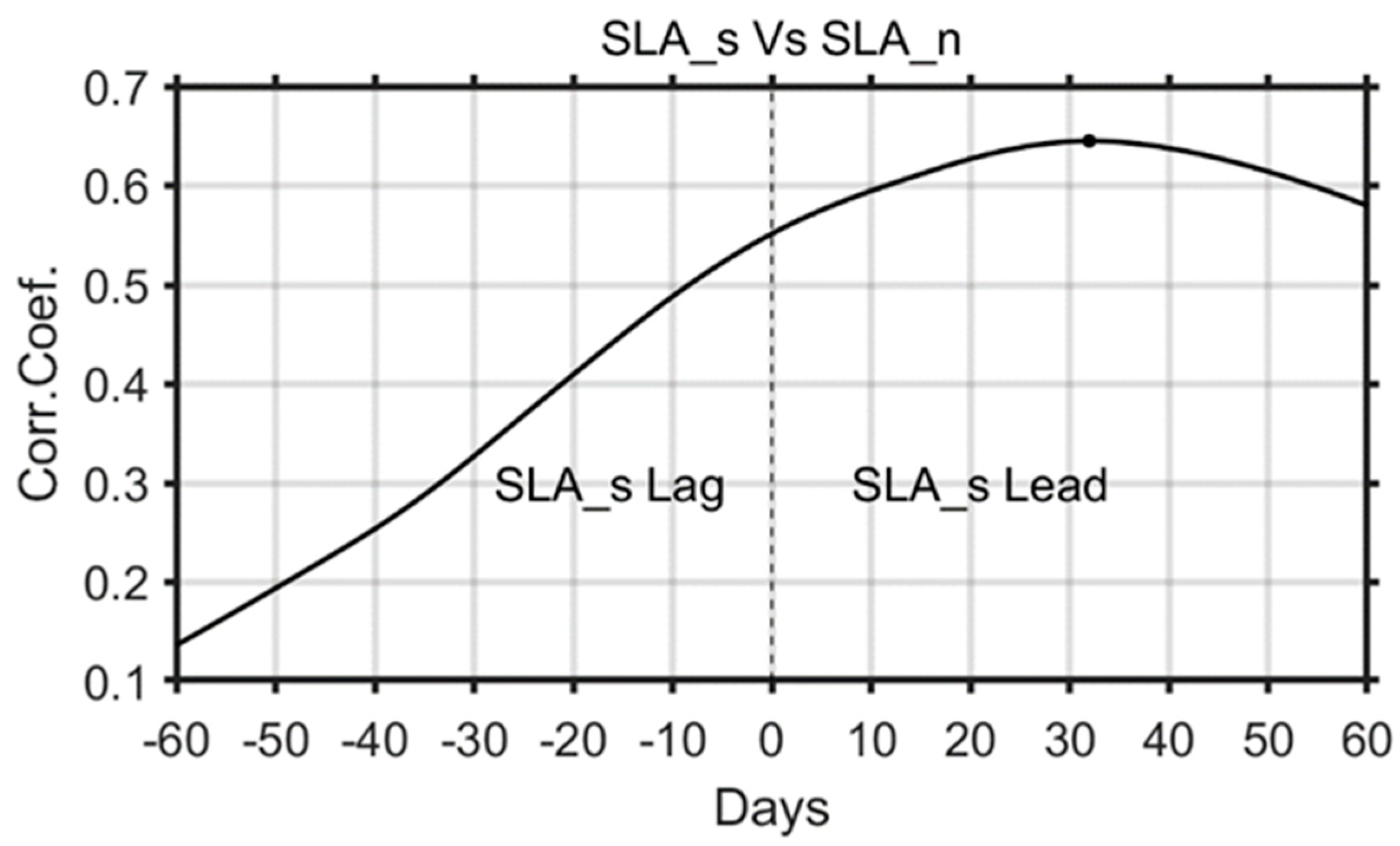
Rao et al. [53] demonstrated that the aforementioned equatorial upwelling (downwelling) Kelvin wave is driven by equatorial easterlies (westerlies) wind. The lead-lag correlation analysis between SLA off the Manaung Island (Station 26 shown in Figure 1a) and that at the central equator (Station 1 shown in Figure 1a) shows that the correlation coefficient is positive and reaches maximum of 0.64 (significant at 99% confidence level) when variation of SLA at Manaung Island (SLA_n) lags behind SLA in the central equator (SLA_s) by 32 days (Figure 7). This means that it takes about 32 d for the signal of SLA variations propagating from the central equator to the Manaung Island. The mean propagation speed of the equatorial Kelvin wave or the coastal Kelvin wave is approximately 1.69 m s−1, close to the typical speed of the second baroclinic mode (1.79 m s−1) [50,54].
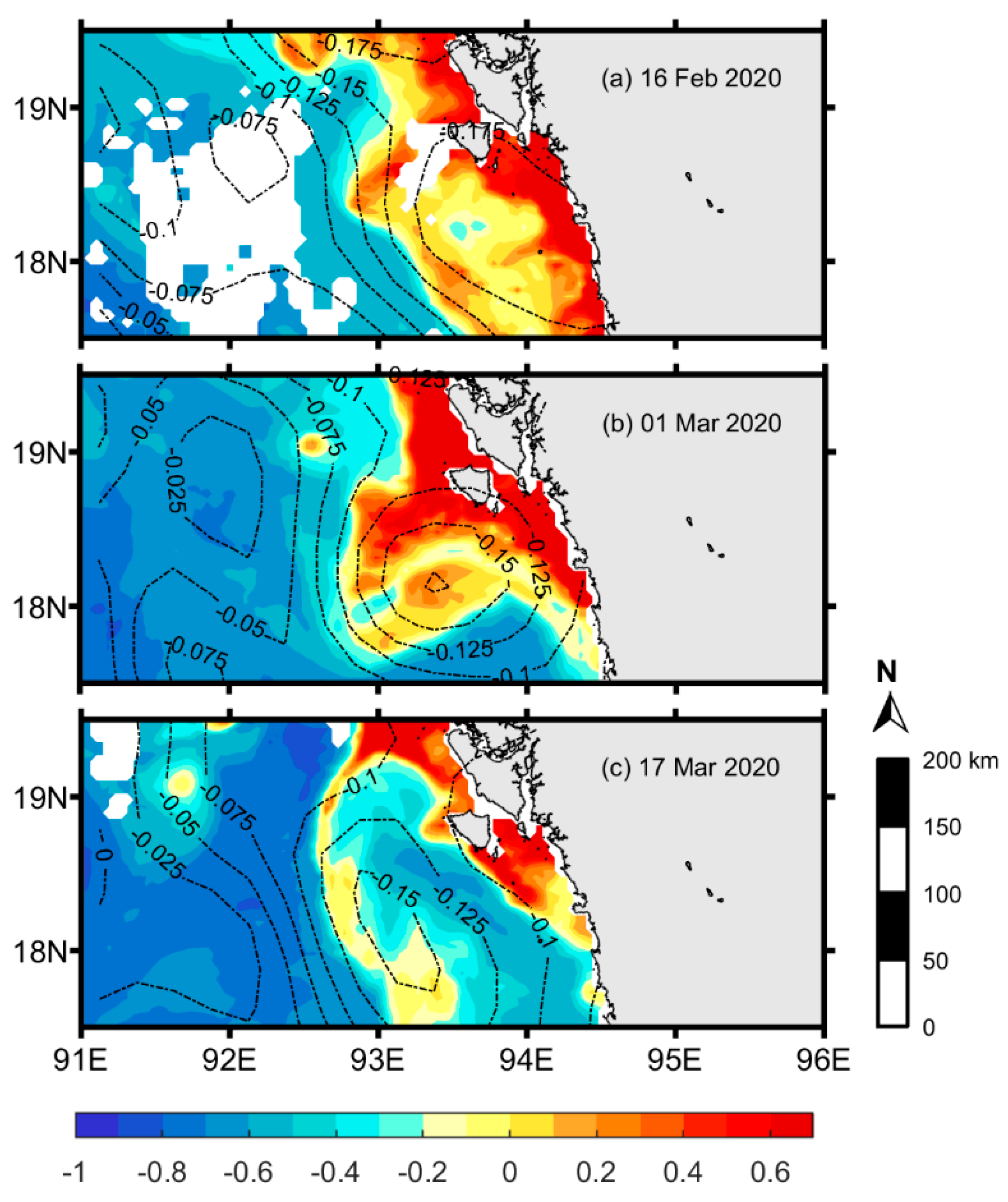
The above analysis has demonstrated that both local wind and equatorial forcing have important impacts on the formation and evolution of the coastal upwelling of Manaung Island. The concentration of Chl-a is another important indicator of the upwelling intensity [43]. The MODIS images of Chl-a for the upwelling period between February and March in 2020 (Figure 8) demonstrate that the short-term evolution of Chl-a distribution in the upwelling zone off Manaung Island is consistent with that of SLA. This consistency underpins that both Chl-a and SLA can well characterize in the intensity of the coastal upwelling of Manaung Island.
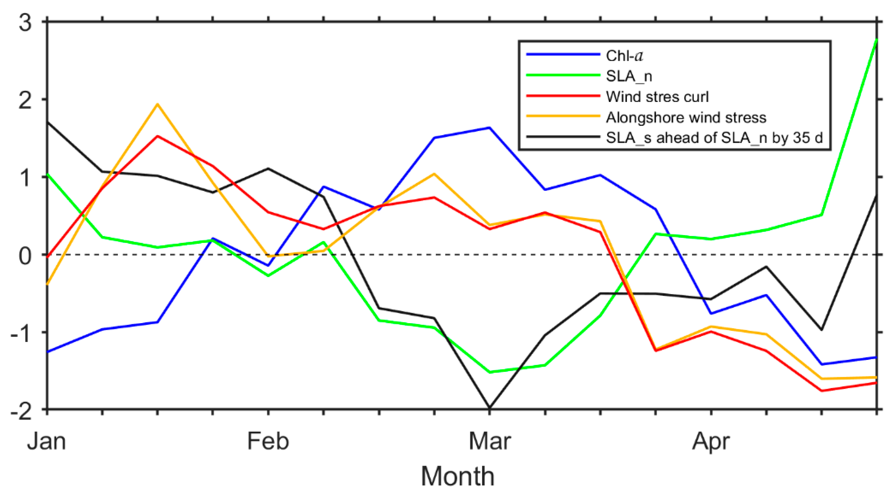
The daily MODIS Chl-a data in the core area of upwelling (the red box in Figure 2c), from January to April, between 2003 and 2020, were composited and then bin-averaged to obtain the climatologically weekly averaged Chl-a time series from January to April. The SLA_n, SLA_s, alongshore wind stress, and wind stress curl were also analyzed using the same method. Then, all these time series were normalized by 1 standard deviation of each (Figure 9). The concentration of Chl-a in the upwelling zone (blue line) continues to increase from January, reaching its peak in early March, and then it decreases during late March and throughout April (Figure 9). This evolution pattern is consistent with variations in the upwelling intensity revealed by the WOA18 temperature and salinity data. As there is a significant correlation between Chl-a concentration and SLA_n with a correlation coefficient of −0.76, SLA_n serves as a good indicator for the intensity of the upwelling at Manaung Island. Thus, the relative contribution of each influencing factor to variations in the upwelling was evaluated by calculating its correlation with SLA_n. The results of correlation analysis (Table 1) demonstrate that there is a high positive correlation between weekly SLA_n and the weekly SLA_s with SLA_s leading SLA_n by 35 days, and their correlation coefficient is 0.60, significant at 95% confidence level. In contrast, SLA_n is negatively correlated with alongshore wind stress and local wind stress curl, with correlation coefficients of −0.35 and −0.33, respectively. These two correlations are not statistically significant (p > 0.05), which indicates that the local wind stress in the upwelling region of Manaung Island has a relatively small impact on the variation in SLA_n. Therefore, the correlation between SLA_n and the equatorial forcing is much stronger than the local wind (0.60 vs. −0.35/−0.33), underpinning that although both local wind and equatorial forcing have impacts on evolution of the upwelling at Manaung Island, the remote forcing from the equator plays a more important role than the local wind does.
5. Discussions
In the upwelling region, upwelled supplies of nitrate and the tremendous blooms of phytoplankton they support, render these regimes the “marine ranchings” [55]. This phytoplankton biomass then feeds into productive food chains which support a significant share of the biological resources that humans harvest from the ocean, and indeed, attract commercial fishers and fisheries [56]. Therefore, the coastal upwelling has a profound impact on coastal populations, and it is particularly important for developing countries (e.g., Myanmar). Despite of the importance of the upwelling, until now, little has been known about the coastal upwelling off Myanmar. This is mainly due to the sparseness of observational data and to the multi-scale aspects of upwelling that are difficult to measure and simulate in climate/ocean models.
Our analysis demonstrates that the center of the upwelling is located at the coastal region off Manaung Island during spring. This is generally consistent with the location of the upwelling reported in the previous studies [30,32,33]. However, seasonal evolution characteristics were not discussed in these previous works due to the scatted measurements from a single cruise used in these studies. In contrast, our study indicates that the upwelling generates in February, then peaks in March and finally decays in May. Based on the satellite observations, the influence of local winds and remote equatorial forcing on the evolution of the upwelling is further discussed by the correlation analysis for the first time. Nevertheless, the physical mechanisms of the upwelling are preliminary. Models will be helpful to isolate the dynamics and assess the relative contribution of various processes in the future study. Our results would contribute to the understanding of coastal processes (including the coastal upwelling) off Myanmar and regional climate variability and their prediction.
Note that the Indian Ocean Dipole (IOD) and El Niño and Southern Oscillation (ENSO) are major climate modes that affect the interannual variability in the northern Indian Ocean [57,58,59]. They can cause interannual variabilities in the regional upwelling in the Indian Ocean by inducing variations in the sea surface wind field [59,60]. For example, significantly interannual variability of the Java–Sumatra upwelling is primarily driven by local winds and remote equatorial Indian Ocean winds associated with IOD/ENSO events [9,18,61]. As our analysis has shown, the coastal upwelling off Myanmar is mainly caused by the remote equatorial forcing and to a lesser degree by the local winds. Both these two forcing indicate significant interannual variabilities caused by IOD and ENSO events [58]. However, how and to what extent the IOD and ENSO events affect the interannual variabilities of the upwelling off Myanmar are still unknown and await further study. A series of cruises are suggested to be carried out in the upwelling region off Myanmar coasts during normal years and IOD/ENSO years to address these important scientific issues.
6. Conclusions
In this paper, WOA18 temperature and salinity datasets, combined with the MODIS Chl-a data, SLA and the CCMP wind data, were used to analyze the spatial structure and seasonal evolution of the coastal upwelling around the Manaung Island. Possible dynamic mechanisms leading to the evolution process of the upwelling were also explored for the first time. The upwelling near the Manaung Island has been identified, which begins in February, reaches its peak in March and disappears in May. Low-temperature (<28.3 °C) and high-salinity (>31.8 psu) water at the surface of this upwelling zone mainly upwells from a depth of 100 m. The impact of upwelling on temperature is found to be more significant in the subsurface layer than that in the surface layer. In contrast, the impact of upwelling on salinity in the surface layer is more significant. This different effect of the upwelling on the temperature and salinity in upper layer is possibly caused by the strong salinity stratification there.
During winter and spring, the local wind near the Manaung Island is dominated by northwesterly/northerly wind. It tends to induce offshore transport in the upper water volume, and consequently is favorable to the formation of coastal upwelling. In addition, the upwelling Kelvin wave, driven by the equatorial easterly wind stress during January-March, propagates along the eastern boundary of the Bay of Bengal, which promotes uplifting of the thermocline and halocline in the coastal regions around the Manaung Island, further enhancing the upwelling. In April, the downwelling Kelvin wave, propagating into the eastern boundary of the Bay from the equator, deepens the thermocline in the waters around the Manaung Island, and simultaneously the local wind is weakening. Both these factors may play an important role in the dissipation of upwelling in this area. Correlation analysis further demonstrates that the remote equatorial forcing exerts a more significant effect on the upwelling variability than the local wind does. Although our study is qualitative, the physical processes are robust features of this region and their quantification will be a major challenge for future observational as well as modeling studies.
Despite the joint effects of remote equatorial forcing and local wind can well explain the generation and evolution of the coastal upwelling around the Manaung Island, we note that the center of the upwelling is located at the Manaung Island where the offshore bottom topography near the Manaung Island has the largest gradient towards the coast. This sharp change in topography may have a significant impact on the distribution of the upwelling center [62], which awaits further analysis in the future.
Author Contributions
Conceptualization, Y.Q.; methodology, Y.Q. and Y.L.; validation, Y.Q. and Y.L.; formal analysis, Y.L.; data curation, Y.Q. and Y.L.; writing—original draft preparation, Y.L. and Y.Q.; writing—review and editing, Y.Q., J.H., C.A., X.L., Y.D.; visualization, Y.L.; funding acquisition, Y.Q. All authors have read and agreed to the published version of the manuscript.
Funding
This study is supported by grants from the Scientific Research Foundation of Third Institute of Oceanography, Ministry of Natural Resources (Nos. 2018001, 2018030 and 2017012); the Ministry of Natural Resources Program on Global Change and Air-Sea interactions (Nos. GASI-IPOVAI-02 and GASI-IPOVAI-03); the National Natural Science Foundation of China (Nos. 41776027, 41906013 and 41276034).
Acknowledgments
We benefited from numerous datasets made freely available, including MODIS data, WOA18 dataset, CCMP wind and CMEMS products.
Conflicts of Interest
The authors declare no conflict of interest.
References
- Nigam, T.; Pant, V.; Prakash, K.R. Impact of Indian ocean dipole on the coastal upwelling features off the southwest coast of India. Ocean Dyn. 2018, 68, 663–676. [Google Scholar] [CrossRef]
- Ryther, J.H. Photosynthesis and fish production in the sea. Science 1969, 166, 72–76. [Google Scholar] [CrossRef] [Green Version]
- Sreeush, M.G.; Valsala, V.; Pentakota, S.; Prasad, K.V.S.R.; Murtugudde, R. Biological production in the Indian Ocean upwelling zones—Part 1: Refined estimation via the use of a variable compensation depth in ocean carbon models. Biogeosciences 2018, 15, 1895–1918. [Google Scholar] [CrossRef] [Green Version]
- Sardeshmukh, P.D.; Hoskins, B.J. The generation of global rotational flow by steady idealized tropical divergence. J. Atmos. Sci. 1988, 45, 1228–1251. [Google Scholar] [CrossRef] [Green Version]
- Webster, P.J.; Lukas, R. TOGA COARE: The coupled ocean atmosphere response experiment. Bull. Am. Meteorol. Soc. 1992, 73, 1377–1416. [Google Scholar] [CrossRef] [Green Version]
- Yu, J.-Y.; Mechoso, C.R.; McWilliams, J.C.; Arakawa, A. Impacts of the Indian Ocean on the ENSO cycle. Geophys. Res. Lett. 2002, 29, 1204. [Google Scholar] [CrossRef] [Green Version]
- Izumo, T.; Vialard, J.; Lengaigne, M.; Montegut, C.D.B.; Behera, S.K.; Luo, J.-J.; Cravatte, S.; Masson, S.; Yamagata, T. Influence of the state of the Indian Ocean Dipole on the following year’s El Niño. Nat. Geosci. 2010, 3, 168–172. [Google Scholar] [CrossRef] [Green Version]
- Kim, S.T.; Yu, J.Y.; Lu, M.M. The distinct behaviors of Pacific and Indian Ocean warm pool properties on seasonal and interannual time scales. J. Geophys. Res. 2012, 117, D05128. [Google Scholar] [CrossRef] [Green Version]
- Zhang, X.L.; Han, W.Q. Effects of climate modes on interannual variability of upwelling in the tropical Indian Ocean. J. Clim. 2020, 33, 1547–1573. [Google Scholar] [CrossRef]
- Colwell, R.R. Global climate and infectious disease: The cholera paradigm. Science 1996, 274, 2025–2031. [Google Scholar] [CrossRef] [Green Version]
- Harwell, C.; Kim, K.; Burkholder, J.; Colwell, R.; Epstein, P.R.; Grimes, D.; Hofmann, E.E.; Lipp, E.K.; Osterhaus, A.; Overshreet, R.M. Emerging marine diseases-climate links and anthropogenic factors. Science 1999, 285, 1505–1510. [Google Scholar] [CrossRef] [PubMed] [Green Version]
- Varkey, M.J.; Murty, V.S.N.; Suryanarayana, A. Physical oceanography of the bay of Bengal and Andaman Sea. Oceanogr. Mar. Biol. Annu. Rev. 1996, 34, 1–70. [Google Scholar]
- Liu, H.X.; Ke, Z.X.; Song, X.Y.; Tan, Y.H.; Huang, L.M.; Lin, Q. Primary production in the Bay of Bengal during spring intermonsoon period. Acta Ecol. Sin. 2011, 31, 7007–7012. [Google Scholar] [CrossRef]
- Prasanna Kumar, S.; Muraleedharan, P.M.; Prasad, T.G.; Gauns, M.; Ramaiah, N.; de Souza, S.N.; Sardesai, S.; Madhupratap, M. Why is the Bay of Bengal less productive during summer monsoon compared to the Arabian Sea? Geophys. Res. Lett. 2002, 29. [Google Scholar] [CrossRef] [Green Version]
- Shetye, S.R.; Shenoi, S.S.C.; Gouveia, A.D.; Michael, G.S.; Sundar, D.; Nampoothiri, G. Wind driven coastal upwelling along the western boundary of the Bay of Bengal during the southwest monsoon. Cont. Shelf Res. 1991, 11, 1397–1408. [Google Scholar] [CrossRef]
- Rao, S.A.; Gopalakrishna, V.V.; Shetye, S.R.; Yamagata, T. Why were cool SST anomalies absent in the Bay of Bengal during the 1997 Indian Ocean Dipole Event? Geophys. Res. Lett. 2002, 29. [Google Scholar] [CrossRef] [Green Version]
- Susanto, R.D.; Gordon, A.L.; Zheng, Q.N. Upwelling along the coasts of Java and Sumatra and its relation to ENSO. Geophys. Res. Lett. 2001, 28, 1599–1602. [Google Scholar] [CrossRef]
- Chen, G.X.; Han, W.Q.; Li, Y.L.; Wang, D.X.; Shinoda, T. Intraseasonal variability of upwelling in the equatorial Eastern Indian Ocean. J. Geophys. Res. 2015, 120, 7598–7615. [Google Scholar] [CrossRef] [Green Version]
- Li, Y.H.; Qiu, Y.; Hu, J.Y.; Aung, C.; Lin, X.Y.; Jing, C.S.; Zhang, J.P. The strong upwelling event in the southern coast of Sri Lanka in 2013 and its relationship with Indian Ocean Dipole events. J. Clim. 2020. under review. [Google Scholar]
- Vinayachandran, P.N.; Chauhan, P.; Mohan, M.; Nayak, S. Biological response of the sea around Sri Lanka to summer monsoon. Geophys. Res. Lett. 2004, 31, L01302. [Google Scholar] [CrossRef]
- De Vos, A.; Pattiaratchi, C.; Wijeratne, E. Surface circulation and upwelling patterns around Sri Lanka. Biogeosciences 2014, 11, 5909. [Google Scholar] [CrossRef] [Green Version]
- Vinayachandran, P.N.; Yamagata, T. Monsoon response of the sea around Sri Lanka: Generation of thermal domes and anticyclonic vortices. J. Phys. Oceanogr. 1998, 28, 1946–1960. [Google Scholar] [CrossRef]
- Burns, J.M.; Subrahmanyam, B.; Murty, V.S.N. On the dynamics of the Sri Lanka Dome in the Bay of Bengal. J. Geophys. Res. Oceans 2017, 122, 7737–7750. [Google Scholar] [CrossRef]
- Cullen, K.E.; Shroyer, E.L. Seasonality and interannual variability of the Sri Lanka dome. Deep Sea Res. II 2019, 168, 104642. [Google Scholar] [CrossRef]
- Murty, C.S.; Varadachari, V.V.R. Upwelling along the east coast of India. Bull. Natl. Inst. Sci. India 1968, 36, 80–86. [Google Scholar]
- Anand, S.P.; Murty, C.B.; Jayaraman, R.; Aggarwal, B.M. Distribution of temperature and oxygen in the Arabian Sea and Bay of Bengal during the monsoon season. Bull. Natl. Inst. Sci. India 1968, 38, 1–24. [Google Scholar]
- De Souza, S.N.; Naqvi, S.W.A.; Reddy, C.V.G. Distribution of nutrients in the western Bay of Bengal. Indian J. Mar. Sci. 1981, 10, 327–331. [Google Scholar]
- Yapa, K.K.A.S. Upwelling phenomena in the southern coastal waters of Sri Lanka during southwest monsoon period as seen from MODIS. Sri. Lanka J. Phys. 2009, 10, 7–15. [Google Scholar] [CrossRef]
- Yesaki, M.; Jantarapagdee, P. Wind stress and sea temperature changes off the west coast of Thailand. In Special Publication on the Occasion of the Tenth Anniversary; Marine Biological Centre: Phuket, Thailand, 1981; pp. 27–42. [Google Scholar]
- Lafond, E.C.; Lafond, K.G. Studies on oceanic circulation in the Bay of Bengal. Bull. Natl. Inst. Sci. India 1968, 38, 164–183. [Google Scholar]
- Rao, D.P. A comparative study of some physical processes governing the potential productivity of the Bay of Bengal and Arabian Sea. Ph.D. Thesis, Andhra University, Waltair, India, 1977. [Google Scholar]
- Suwannathatsa, S.; Wongwises, P.; Vongvisessomjai, S.; Wannawong, W.; Saetae, D. Phytoplankton tracking by oceanic model and satellite data in the Bay of Bengal and Andaman Sea. APCBEE Procedia 2012, 2, 183–189. [Google Scholar] [CrossRef] [Green Version]
- Akester, M.J. Productivity and coastal fisheries biomass yields of the northeast coastal waters of the Bay of Bengal Large Marine Ecosystem. Deep Sea Res. Part II Top. Stud. Oceanogr. 2019, 163, 46–56. [Google Scholar] [CrossRef]
- Zweng, M.M.; Reagan, J.R.; Seidov, D.; Boyer, T.P.; Locarnini, R.A.; Garcia, H.E.; Mishonov, A.V.; Baranova, O.K.; Weathers, K.W.; Paver, C.R.; et al. World Ocean Atlas 2018, Volume 2: Salinity; A. Mishonov Technical, Ed.; Silver Spring, Department of Commerce: Montgomery, MD, USA, 2018.
- Locarnini, R.A.; Mishonov, A.V.; Baranova, O.K.; Boyer, T.P.; Zweng, M.M.; Garcia, H.E.; Reagan, J.R.; Seidov, D.; Weathers, K.W.; Paver, C.R.; et al. World Ocean Atlas 2018. Volume 1: Temperature; A. Mishonov Technical, Ed.; Silver Spring, Department of Commerce: Montgomery, MD, USA, 2018.
- O’Reilly, J.E.; Maritorena, S.; Mitchell, B.; Siegel, D.; Carder, K.; Garver, S.; Kahru, M.; McClain, C. Ocean color chlorophyll algorithms for SeaWiFS. J. Geophys. Res. Ocean 1998, 103, 24937–24953. [Google Scholar] [CrossRef] [Green Version]
- Cui, T.W.; Zhang, J.; Tang, J.W.; Sathyendranath, S.; Groom, S.; Ma, Y.; Zhao, W.; Song, Q.J. Assessment of satellite ocean color products of MERIS, MODIS and SeaWiFS along the East China Coast (in the Yellow Sea and East China Sea). J. Photogramm. Remote Sens. 2014, 87, 137–151. [Google Scholar] [CrossRef]
- Esaias, W.E.; Abbott, M.R.; Barton, I.; Brown, O.B.; Campbell, J.W.; Carder, K.L.; Clark, D.K.; Evans, R.H.; Hoge, F.E.; Gordon, H.R.; et al. An overview of MODIS capabilities for ocean science observations. IEEE Trans. Geosci. Remote 1998, 36, 1250–1265. [Google Scholar] [CrossRef] [Green Version]
- Atlas, R.; Hoffman, R.N.; Ardizzone, J.; Leidner, S.M.; Jusem, J.C.; Smith, D.K.; Gombos, D. A cross-calibrated, multiplatform ocean surface wind velocity product for meteorological and oceanographic applications. Bull. Amer. Meteor. Soc. 2011, 92, 157–174. [Google Scholar] [CrossRef]
- Ducet, N.; Traon, P.Y.L.; Reverdin, G. Global high-resolution mapping of ocean circulation from TOPEX/Poseidon and ERS-1 and -2. J. Geophys. Res. 2000, 105, 19477–19498. [Google Scholar] [CrossRef]
- Jing, Z.Y.; Qi, Y.Q.; Du, Y. Upwelling in the continental shelf of northern South China Sea associated with 1997–1998 El Niño. J. Geophys. Res 2011, 116, C02033. [Google Scholar] [CrossRef]
- Akhir, M.F.; Daryabor, F.; Husain, M.L.; Tangang, F.; Qiao, F.L. Evidence of upwelling along peninsular malaysia during Southwest Monsoon. Open J. Mar. Sci. 2015, 5, 273–279. [Google Scholar] [CrossRef] [Green Version]
- Xie, S.P.; Xie, Q.; Wang, D.X.; Liu, W.T. Summer upwelling in the South China Sea and its role in regional climate variations. J. Geophys. Res. 2003, 108. [Google Scholar] [CrossRef] [Green Version]
- Thangaprakash, V.P.; Girishkumar, M.S.; Suprit, K.; Suresh Kumar, N.; Chaudhuri, D.; Dinesh, K.; Kumar, A.; Shivaprasad, S.; Ravichandran, M.; Thomas Farrar, J.; et al. What controls seasonal evolution of sea surface temperature in the Bay of Bengal? Oceanography 2016, 29, 202–213. [Google Scholar] [CrossRef] [Green Version]
- Li, K.P.; Wang, H.Y.; Yang, Y.; Yu, W.D.; Li, L.L. Observed characteristics and mechanisms of temperature inversion in the northern Bay of Bengal. Acta Oceanol. Sin. 2016, 38, 22–31. [Google Scholar] [CrossRef]
- Qiu, Y.; Li, L. Annual variation of geostrophic circulation in the Bay of Bengal observed with TOPEX/Poseidon altimeter data. Acta Oceanol. Sin. 2007, 29, 39–46. [Google Scholar]
- Hu, J.Y.; Kawamura, H.; Hong, H.S.; Pan, W.R. A review of research on the upwelling in the Taiwan strait. Bull. Mar. Sci. 2003, 73, 605–628. [Google Scholar]
- Price, J.F.; Weller, R.A.; Schudlich, R.R. Wind-driven ocean currents and Ekman transport. Science 1987, 238, 1534–1538. [Google Scholar] [CrossRef] [Green Version]
- Han, W.Q.; Webster, P.J. Forcing mechanisms of sea level interannual variability in the Bay of Bengal. J Phys. Oceanogr. 2002, 32, 216–239. [Google Scholar] [CrossRef] [Green Version]
- Cravatte, S.; Picaut, J.; Eldin, G. Second and first baroclinic Kelvin modes in the equatorial Pacific at intraseasonal timescales. J. Geophys. Res. Oceans 2003, 108, 3266. [Google Scholar] [CrossRef]
- Cheng, X.H.; Xie, S.P.; Mccreary, J.P. Intraseasonal variability of sea surface height in the Bay of Bengal. J. Geophys. Res. Oceans 2013, 188, 816–830. [Google Scholar] [CrossRef]
- Cheng, X.H.; Mccreary, J.P.; Qiu, B. Intraseasonal-to-semiannual variability of sea-surface height in the astern, equatorial Indian Ocean and Southern Bay of Bengal. J. Geophys. Res. Oceans 2017, 122, 4051–4067. [Google Scholar] [CrossRef]
- Rao, R.R.; Girish Kumar, M.S.; Ravichandran, M.; Rao, A.R.; Gopalakrishna, V.V.; Thadathil, P. Interannual variability of Kelvin wave propagation in the wave guides of the equatorial Indian Ocean, the coastal Bay of Bengal and the southeastern Arabian Sea during 1993–2006. Deep Sea Res. Part I Oceanogr. Res. Pap. 2010, 57, 1–13. [Google Scholar] [CrossRef]
- Gent, P.R.; O’Neill, K.; Cane, M.A. A model of the semiannual oscillation in the Equatorial Indian Ocean. J. Phys. Oceanogr. 1983, 13, 148. [Google Scholar] [CrossRef] [Green Version]
- Huang, B.Q.; Xiang, W.G.; Zeng, X.B.; Chiang, K.P.; Tian, H.J.; Hu, J.; Lan, W.L.; Hong, H.S. Phytoplankton growth and microzooplankton grazing in a subtropical coastal upwelling system in the Taiwan Strait. Cont. Shelf Res. 2011, 31, S48–S56. [Google Scholar] [CrossRef]
- Pauly, D.; Christensen, V. Primary production required to sustain global fisheries. Nature 1995, 374, 255–257. [Google Scholar] [CrossRef]
- Saji, N.H.; Goswami, B.N.; Vinayachandran, P.N.; Yamagata, T. A dipole mode in the tropical Indian Ocean. Nature 1999, 401, 360–363. [Google Scholar] [CrossRef]
- Yu, W.D.; Xiang, B.Q.; Liu, L.; Liu, N. Understanding the origins of interannual thermocline variations in the tropical Indian Ocean. Geophys. Res. Lett. 2005, 32, L24706. [Google Scholar] [CrossRef]
- Saji, N.H.; Yamagata, T. Possible impacts of Indian Ocean Dipole mode events on global climate. Clim. Res. 2003, 25, 151–169. [Google Scholar] [CrossRef]
- Anil, N.; Kumar, M.R.R.; Sajeev, R.; Saji, P.K. Role of distinct flavours of IOD events on Indian summer monsoon. Nat. Hazards 2016, 82, 1317–1326. [Google Scholar] [CrossRef]
- Horii, T.; Ueki, I.; Ando, K. Coastal upwelling events along the southern coast of Java during the 2008 positive Indian Ocean Dipole. J. Oceanogr. 2008, 74, 499–508. [Google Scholar] [CrossRef]
- Gan, J.P.; Cheung, A.; Guo, X.G.; Li, L. Intensified upwelling over a widened shelf in the northeastern South China Sea. J. Geophys. Res. 2009, 114, C09019. [Google Scholar] [CrossRef]
Figure 1.
(a) Geographical location of the Bay of Bengal, and (b) topography of the northwestern coasts of Myanmar. The blue line in Figure 1a indicates the propagation path of the equatorial Kelvin wave and coastal Kelvin wave. The red dots in the blue line denote the selected stations of sea level anomaly (SLA) to track the propagation of Kevin wave along the equator and eastern boundary of the Bay. In Figure 1a, the India coastal upwelling, Sri Lanka coastal upwelling, Sri Lanka Cold Eddy and Sri Lanka are denoted by ICU, SLCU, SLCE and SL, respectively. In Figure 1b, the red box represents the study region A (91.0–93.5° E, 18.5–19.0° N), and the black contours are the isobaths of 50, 200, 1500 and 2000 m.

Figure 2.
Sample amounts of surface temperature (a) and salinity (b) in spring (March-May) in a 1° × 1° grid; (c) and (d) are climatological surface temperature (unit: °C) and salinity (unit: psu) in the same period. In Figure 2c, the dotted lines indicate the locations of Section 1 (93.375° E, 16.875–19.125° N) and Section 2 (90.125–93.375° E, 18.875° N), the red box (93.0–94.0° E, 18.5–19.0° N) represents the core area of upwelling, and the solid line is the 28.3 °C isotherm. The solid line in Figure 2d is the 31.8 psu isohaline. Temperature and salinity data are from climatological monthly data set of World Ocean Atlas 2018 (WOA18).

Figure 3.
The climatologically sectional distributions of (a) temperature (unit: °C) and (b) salinity (unit: psu) of two sections in spring. The locations of the two sections are shown in Figure 2c.
Figure 3.
The climatologically sectional distributions of (a) temperature (unit: °C) and (b) salinity (unit: psu) of two sections in spring. The locations of the two sections are shown in Figure 2c.

Figure 4.
The climatological distributions of surface temperature (upper panels, unit: °C) and salinity (lower panels, unit: psu) in the waters of Myanmar from February to May. Temperature and salinity are from climatological monthly data of WOA18.
Figure 4.
The climatological distributions of surface temperature (upper panels, unit: °C) and salinity (lower panels, unit: psu) in the waters of Myanmar from February to May. Temperature and salinity are from climatological monthly data of WOA18.

Figure 5.
The climatological distributions of temperature (upper panels, unit: °C) and salinity (lower panels, unit: psu) in the 40, 60 and 80 m layers in the waters of Myanmar in February. Temperature and salinity are from climatological monthly data of WOA18.
Figure 5.
The climatological distributions of temperature (upper panels, unit: °C) and salinity (lower panels, unit: psu) in the 40, 60 and 80 m layers in the waters of Myanmar in February. Temperature and salinity are from climatological monthly data of WOA18.

Figure 6.
(a) Time series of climatological monthly alongshore wind stress of Manaung Island (the southeast direction along the coastline is positive, unit: N m−2); (b) Time–Longitude diagram of climatological monthly wind stress curl averaged over area A (unit: 10−7 N m−3); (c) Time–station diagram of climatological monthly SLA (unit: m). The stations and the range of area A are shown in Figure 1a,b, respectively. All climatological monthly mean data is averaged from the daily/6 h data for the period 1993 to 2016.

Figure 7.
Lead/lag correlation between SLA at Station 26 (SLA_n) and that at Station 1 (SLA_s) using data from January 2003 to December 2016. The x-coordinate represents the number of days, a positive value of which indicates a leading SLA_s, and the y-coordinate represents the correlation coefficient.

Figure 8.
Logarithm (Log10) of Chl-a concentrations (shaded, unit: mg m−3) and SLA (contours, unit: m) in the waters of Manaung Island for (a) 16 February, (b) 1 March, and (c) 17 March in 2020. Blank areas indicate missing data.
Figure 8.
Logarithm (Log10) of Chl-a concentrations (shaded, unit: mg m−3) and SLA (contours, unit: m) in the waters of Manaung Island for (a) 16 February, (b) 1 March, and (c) 17 March in 2020. Blank areas indicate missing data.

Figure 9.
Time series of climatologically weekly Chl-a concentrations, wind stress curl, alongshore wind stress, SLA_n and SLA_s ahead of SLA_n by 35 d from January to April (all data are averaged during 2003–2016 and normalized by one standard deviation).
Figure 9.
Time series of climatologically weekly Chl-a concentrations, wind stress curl, alongshore wind stress, SLA_n and SLA_s ahead of SLA_n by 35 d from January to April (all data are averaged during 2003–2016 and normalized by one standard deviation).


Table 1.
The correlation coefficients between indicator of the upwelling (SLA_n and Chl-a) and forcing factors.
Table 1.
The correlation coefficients between indicator of the upwelling (SLA_n and Chl-a) and forcing factors.
| Indicator of the Upwelling | Indicator of the Upwelling/Forcing Factor | Correlation Coefficient |
|---|---|---|
| SLA_n | Chl-a | −0.76 |
| SLA_n | Wind stress curl | −0.35 |
| SLA_n | SLA_s ahead of SLA_n by 35 days | 0.60 |
| SLA_n | Alongshore wind stress | −0.33 |
Publisher’s Note: MDPI stays neutral with regard to jurisdictional claims in published maps and institutional affiliations. |
© 2020 by the authors. Licensee MDPI, Basel, Switzerland. This article is an open access article distributed under the terms and conditions of the Creative Commons Attribution (CC BY) license (http://creativecommons.org/licenses/by/4.0/).
Share and Cite
MDPI and ACS Style
Li, Y.; Qiu, Y.; Hu, J.; Aung, C.; Lin, X.; Dong, Y. Springtime Upwelling and Its Formation Mechanism in Coastal Waters of Manaung Island, Myanmar. Remote Sens. 2020, 12, 3777. https://0-doi-org.brum.beds.ac.uk/10.3390/rs12223777
AMA Style
Li Y, Qiu Y, Hu J, Aung C, Lin X, Dong Y. Springtime Upwelling and Its Formation Mechanism in Coastal Waters of Manaung Island, Myanmar. Remote Sensing. 2020; 12(22):3777. https://0-doi-org.brum.beds.ac.uk/10.3390/rs12223777
Chicago/Turabian StyleLi, Yuhui, Yun Qiu, Jianyu Hu, Cherry Aung, Xinyu Lin, and Yue Dong. 2020. "Springtime Upwelling and Its Formation Mechanism in Coastal Waters of Manaung Island, Myanmar" Remote Sensing 12, no. 22: 3777. https://0-doi-org.brum.beds.ac.uk/10.3390/rs12223777
Note that from the first issue of 2016, this journal uses article numbers instead of page numbers. See further details here.