Dark Glacier Surface of Greenland’s Largest Floating Tongue Governed by High Local Deposition of Dust

 , , , , , , , , and
Abstract
:
1. Introduction
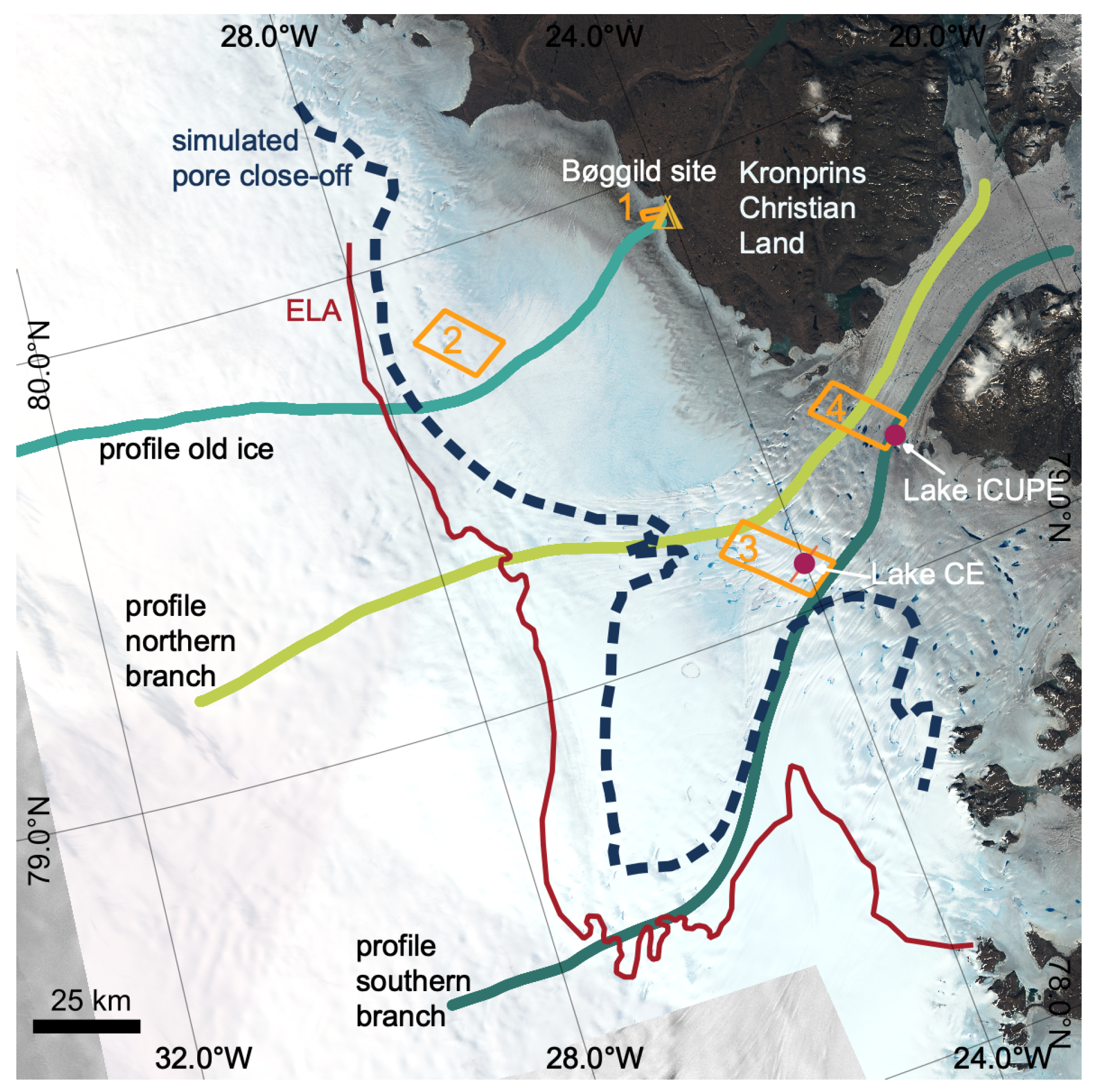
2. Study Site
3. Materials and Methods
3.1. Optical Remote Sensing: MODIS
3.2. Optical Remote Sensing: Sentinel-2
3.3. Radar Remote Sensing: Sentinel-1 Polarimetry
3.4. Roughness
3.5. Firn Modelling
4. Results
4.1. Annual Deposition of Impurities
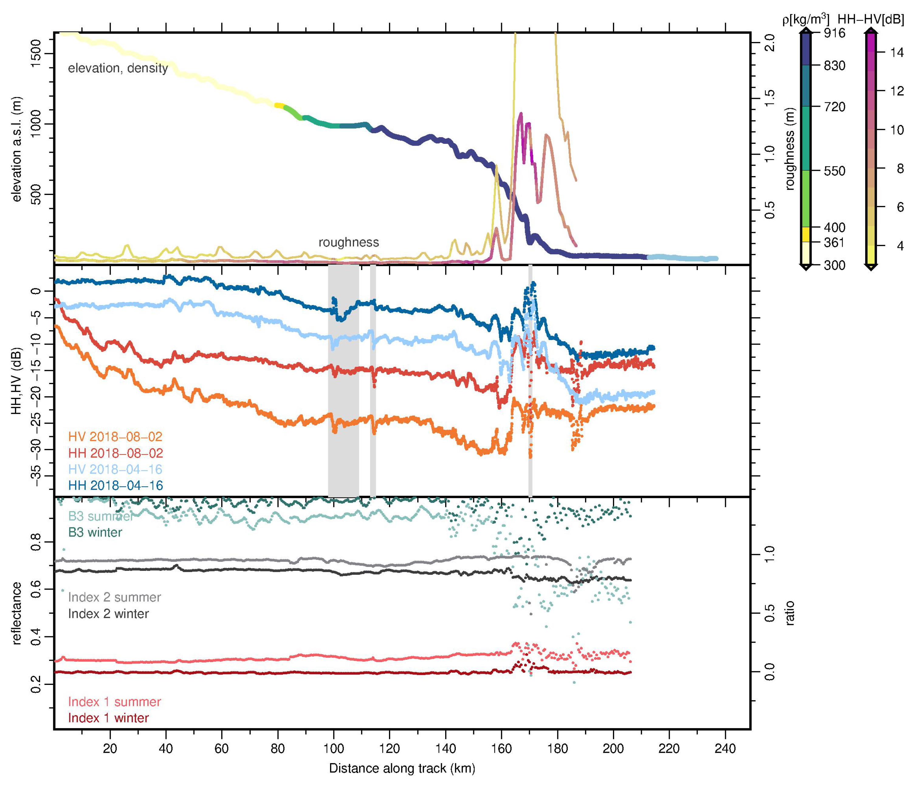
4.2. Profile “Southern Branch”
4.3. Profile “Northern Branch”
4.4. Profile “Old Ice”
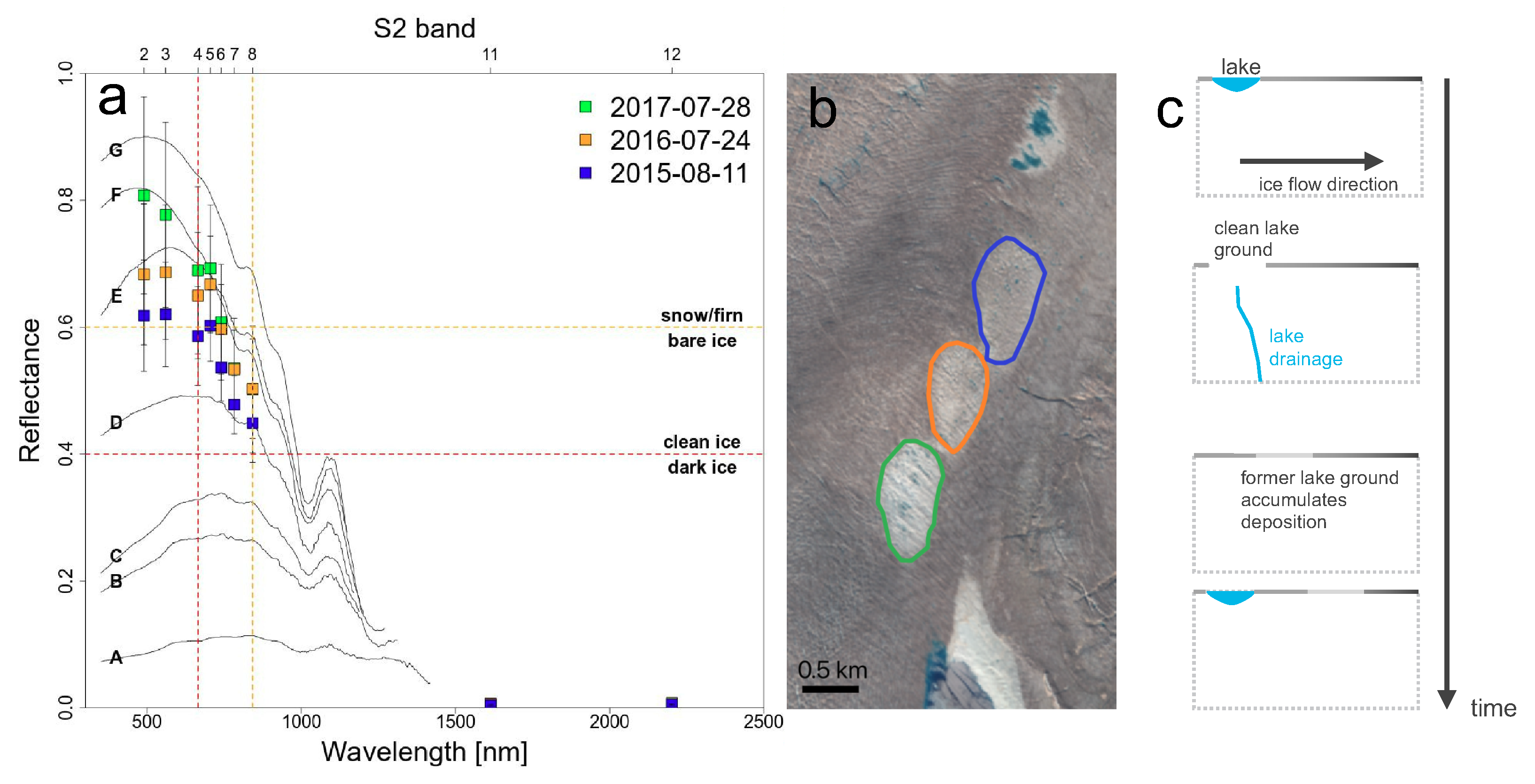
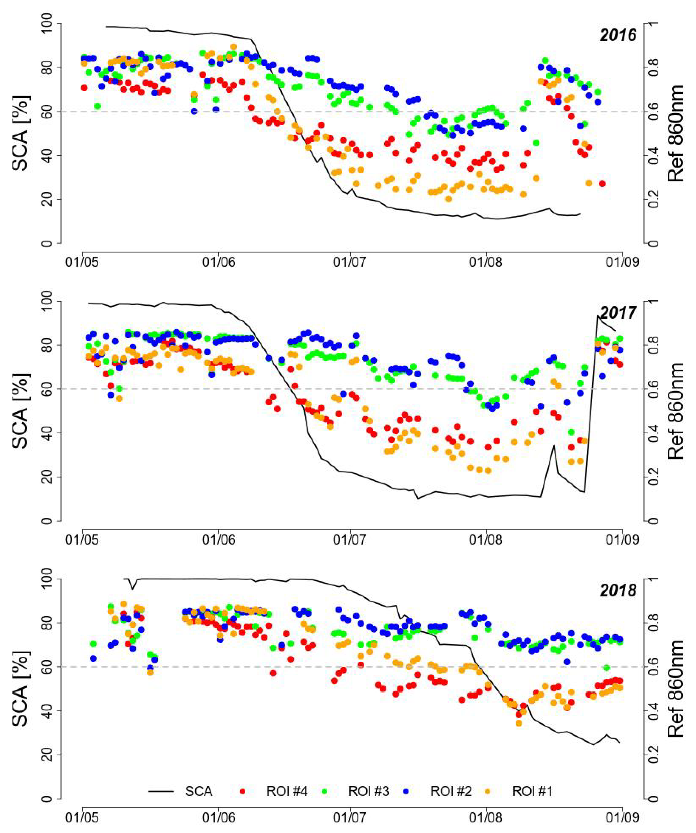
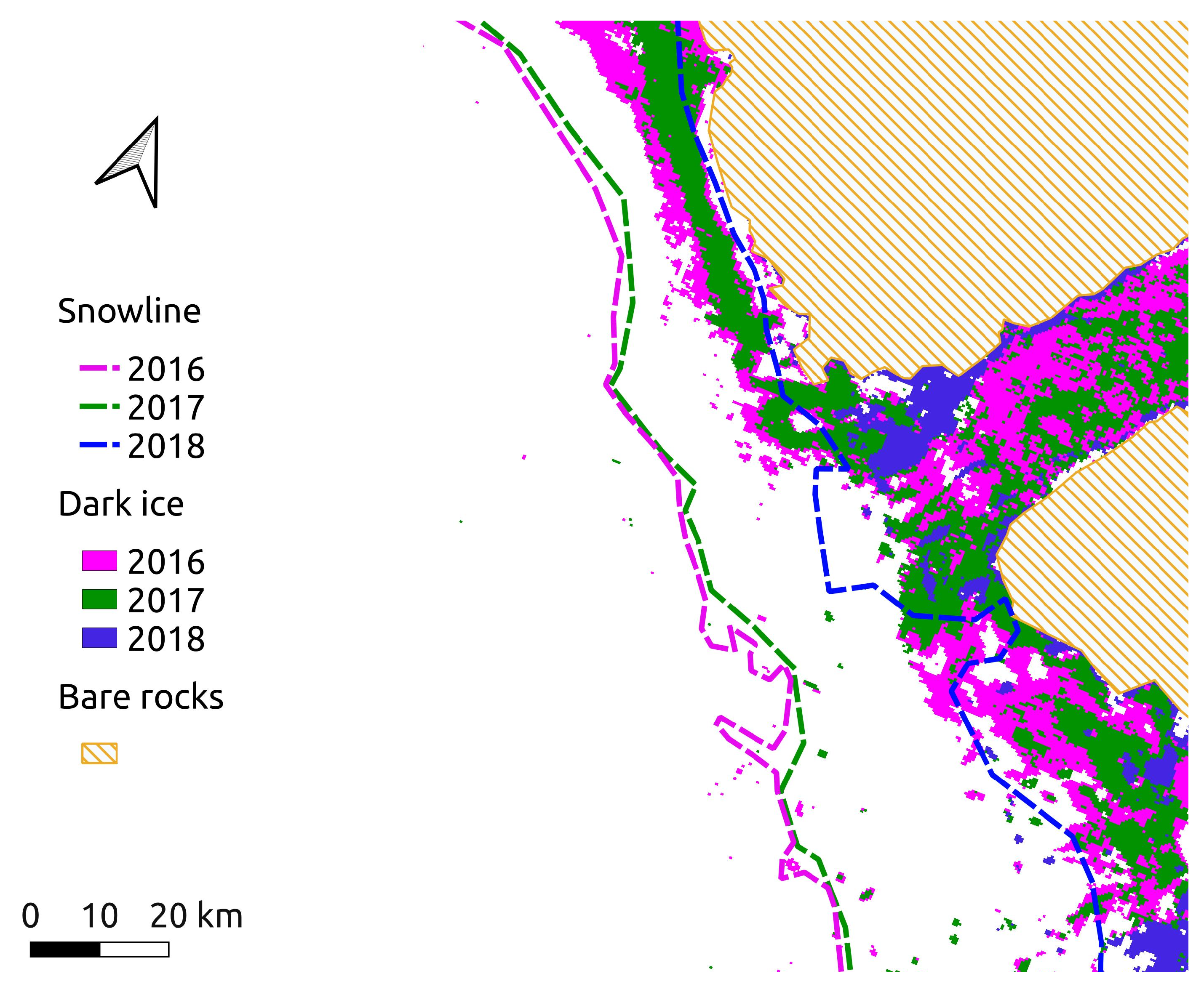
4.5. Snow, Bare and Dark Ice Surface
5. Discussion
6. Conclusions
Supplementary Materials
Author Contributions
Funding
Acknowledgments
Conflicts of Interest
Abbreviations
| 79 NG | 79N Glacier |
| MODIS | Moderate Resolution Imaging Spectroradiometer |
| S1, S2 | Sentinel-1, Sentinel-2 |
| UWB-M | Ultra-Wide-Band-Microwave radar |
| BC | black carbon |
References
- van den Broeke, M.R.; Enderlin, E.M.; Howat, I.M.; Kuipers Munneke, P.; Noël, B.P.Y.; van de Berg, W.J.; van Meijgaard, E.; Wouters, B. On the recent contribution of the Greenland ice sheet to sea level change. Cryosphere 2016, 10, 1933–1946. [Google Scholar] [CrossRef] [Green Version]
- Mouginot, J.; Rignot, E.; Bjørk, A.A.; van den Broeke, M.; Millan, R.; Morlighem, M.; Noël, B.; Scheuchl, B.; Wood, M. Forty-six years of Greenland Ice Sheet mass balance from 1972 to 2018. Proc. Natl. Acad. Sci. USA 2019, 116, 9239–9244. [Google Scholar] [CrossRef] [PubMed] [Green Version]
- Willeit, M.; Ganopolski, A. The importance of snow albedo for ice sheet evolution over the last glacial cycle. Clim. Past 2018, 14, 697–707. [Google Scholar] [CrossRef] [Green Version]
- Tedesco, M.; Doherty, S.; Fettweis, X.; Alexander, P.; Jeyaratnam, J.; Stroeve, J. The darkening of the Greenland ice sheet: Trends, drivers, and projections (1981–2100). Cryosphere 2016, 10, 477–496. [Google Scholar] [CrossRef] [Green Version]
- Schröder, L.; Neckel, N.; Zindler, R.; Humbert, A. Perennial supraglacial lakes in Northeast Greenland observed by polarimetric SAR. Remote Sens. 2020, 12, 2798. [Google Scholar] [CrossRef]
- Selmes, N.; Murray, T.; James, T.D. Fast draining lakes on the Greenland Ice Sheet. Geophys. Res. Lett. 2011, 38. [Google Scholar] [CrossRef]
- Smith, L.C.; Chu, V.W.; Yang, K.; Gleason, C.J.; Pitcher, L.H.; Rennermalm, A.K.; Legleiter, C.J.; Behar, A.E.; Overstreet, B.T.; Moustafa, S.E.; et al. Efficient meltwater drainage through supraglacial streams and rivers on the southwest Greenland ice sheet. Proc. Natl. Acad. Sci. USA 2015, 112, 1001–1006. [Google Scholar] [CrossRef] [Green Version]
- Yang, K.; Smith, L.C. Supraglacial Streams on the Greenland Ice Sheet Delineated From Combined Spectral–Shape Information in High-Resolution Satellite Imagery. IEEE Geosci. Remote Sens. Lett. 2013, 10, 801–805. [Google Scholar] [CrossRef]
- Simonsen, M.F.; Baccolo, G.; Blunier, T. East Greenland ice core dust record reveals timing of Greenland ice sheet advance and retreat. Nat. Commun. 2019, 10. [Google Scholar] [CrossRef] [Green Version]
- Ryan, J.; Hubbard, A.; Stibal, M.; Irvine-Fynn, T.; Cook, J.; Smith, L.C.; Cameron, K.; Box, J. Dark zone of the Greenland Ice Sheet controlled by distributed biologically-active impurities. Nat. Commun. 2018, 9. [Google Scholar] [CrossRef] [Green Version]
- Gardner, A.S.; Sharp, M.J. A review of snow and ice albedo and the development of a new physically based broadband albedo parameterization. J. Geophys. Res. Earth Surf. 2010, 115. [Google Scholar] [CrossRef]
- Ryan, J.; Smith, L.; van As, D.; Cooley, D.; Cooper, M.; Pitcher, L.; Hubbard, A. Greenland Ice Sheet surface melt amplified by snowline migration and bare ice exposure. Sci. Adv. 2019, 5. [Google Scholar] [CrossRef] [PubMed] [Green Version]
- Shimada, R.; Takeuchi, N.; Aoki, T. Inter-Annual and Geographical Variations in the Extent of Bare Ice and Dark Ice on the Greenland Ice Sheet Derived from MODIS Satellite Images. Front. Earth Sci. 2016, 4, 1–10. [Google Scholar] [CrossRef] [Green Version]
- Aoki, T.; Kuchiki, K.; Niwano, M.; Kodama, Y.; Hosaka, M.; Tanaka, T. Physically based snow albedo model for calculating broadband albedos and the solar heating profile in snowpack for general circulation models. J. Geophys. Res. Atmos. 2011, 116. [Google Scholar] [CrossRef]
- Domine, F.; Salvatori, R.; Legagneux, L.; Salzano, R.; Fily, M.; Casacchia, R. Correlation between the specific surface area and the short wave infrared (SWIR) reflectance of snow. Cold Reg. Sci. Technol. 2006, 46, 60–68. [Google Scholar] [CrossRef]
- Warren, S.G. Optical properties of snow. Rev. Geophys. 1982, 20, 67–89. [Google Scholar] [CrossRef]
- He, C.; Flanner, M.G.; Chen, F.; Barlage, M.; Liou, K.N.; Kang, S.; Ming, J.; Qian, Y. Black carbon-induced snow albedo reduction over the Tibetan Plateau: Uncertainties from snow grain shape and aerosol–snow mixing state based on an updated SNICAR model. Atmos. Chem. Phys. 2018, 18, 11507–11527. [Google Scholar] [CrossRef] [Green Version]
- Jacobi, H.W.; Obleitner, F.; Da Costa, S.; Ginot, P.; Eleftheriadis, K.; Aas, W.; Zanatta, M. Deposition of ionic species and black carbon to the Arctic snowpack: Combining snow pit observations with modeling. Atmos. Chem. Phys. 2019, 19, 10361–10377. [Google Scholar] [CrossRef] [Green Version]
- Eleftheriadis, K.; Vratolis, S.; Nyeki, S. Aerosol black carbon in the European Arctic: Measurements at Zeppelin station, Ny-ålesund, Svalbard from 1998–2007. Geophys. Res. Lett. 2009, 36. [Google Scholar] [CrossRef] [Green Version]
- Stone, R.; Sharma, S.; Herber, A.; Eleftheriadis, K.; Nelson, D. A characterization of Arctic aerosols on the basis of aerosol optical depth and black carbon measurements. Elem. Sci. Anthr. 2014, 2. [Google Scholar] [CrossRef] [Green Version]
- Petäjä, T.; Duplissy, E.M.; Tabakova, K.; Schmale, J.; Altstädter, B.; Ancellet, G.; Arshinov, M.; Balin, Y.; Baltensperger, U.; Bange, J.; et al. Integrative and comprehensive Understanding on Polar Environments (iCUPE): The concept and initial results. Atmos. Chem. Phys. Discuss. 2020, 2020, 1–62. [Google Scholar] [CrossRef]
- Collaud Coen, M.; Andrews, E.; Alastuey, A.; Arsov, T.P.; Backman, J.; Brem, B.T.; Bukowiecki, N.; Couret, C.; Eleftheriadis, K.; Flentje, H.; et al. Multidecadal trend analysis of aerosol radiative properties at a global scale. Atmos. Chem. Phys. Discuss. 2020, 2020, 1–54. [Google Scholar] [CrossRef] [Green Version]
- Gong, S.L.; Zhao, T.L.; Sharma, S.; Toom-Sauntry, D.; Lavoué, D.; Zhang, X.B.; Leaitch, W.R.; Barrie, L.A. Identification of trends and interannual variability of sulfate and black carbon in the Canadian High Arctic: 1981–2007. J. Geophys. Res. Atmos. 2010, 115. [Google Scholar] [CrossRef]
- Sharma, S.; Andrews, E.; Barrie, L.A.; Ogren, J.A.; Lavoué, D. Variations and sources of the equivalent black carbon in the high Arctic revealed by long-term observations at Alert and Barrow: 1989–2003. J. Geophys. Res. Atmos. 2006, 111. [Google Scholar] [CrossRef]
- Sharma, S.; Ishizawa, M.; Chan, D.; Lavoué, D.; Andrews, E.; Eleftheriadis, K.; Maksyutov, S. 16-year simulation of Arctic black carbon: Transport, source contribution, and sensitivity analysis on deposition. J. Geophys. Res. Atmos. 2013, 118, 943–964. [Google Scholar] [CrossRef]
- Bond, T.C.; Doherty, S.J.; Fahey, D.W.; Forster, P.M.; Berntsen, T.; DeAngelo, B.J.; Flanner, M.G.; Ghan, S.; Kärcher, B.; Koch, D.; et al. Bounding the role of black carbon in the climate system: A scientific assessment. J. Geophys. Res. Atmos. 2013, 118, 5380–5552. [Google Scholar] [CrossRef]
- Liu, J.; Fan, S.; Horowitz, L.W.; Levy, H., II. Evaluation of factors controlling long-range transport of black carbon to the Arctic. J. Geophys. Res. Atmos. 2011, 116. [Google Scholar] [CrossRef]
- Contini, D.; Donateo, A.; Belosi, F.; Grasso, F.M.; Santachiara, G.; Prodi, F. Deposition velocity of ultrafine particles measured with the Eddy-Correlation Method over the Nansen Ice Sheet (Antarctica). J. Geophys. Res. Atmos. 2010, 115. [Google Scholar] [CrossRef] [Green Version]
- Grönlund, A.; Nilsson, D.; Koponen, I.K.; Virkkula, A.; Hansson, M.E. Aerosol dry deposition measured with eddy-covariance technique at Wasa and Aboa, DronningMaud Land, Antarctica. Ann. Glaciol. 2002, 35, 355–361. [Google Scholar] [CrossRef] [Green Version]
- Doherty, S.J.; Grenfell, T.C.; Forsström, S.; Hegg, D.L.; Brandt, R.E.; Warren, S.G. Observed vertical redistribution of black carbon and other insoluble light-absorbing particles in melting snow. J. Geophys. Res. Atmos. 2013, 118, 5553–5569. [Google Scholar] [CrossRef]
- Bøggild, C.E.; Brandt, R.E.; Brown, K.J.; Warren, S.G. The ablation zone in northeast Greenland: Ice types, albedos and impurities. J. Glaciol. 2010, 56, 101–113. [Google Scholar] [CrossRef] [Green Version]
- Wager, A.C. Flooding of the ice shelf in the GeorgVI sound. Br. Antarct. Surv. Bull. 1972, 28, 71–74. [Google Scholar]
- Krieger, L.; Floricioiu, D.; Neckel, N. Drainage basin delineation for outlet glaciers of Northeast Greenland based on Sentinel-1 ice velocities and TanDEM-X elevations. Remote Sens. Environ. 2020, 237, 111483. [Google Scholar] [CrossRef]
- Hall, D.; Riggs, G. MODIS/Terra Snow Cover Daily L3 Global 500m SIN Grid, Version 6. 2016. Available online: https://nsidc.org/data/MOD10A1/versions/6 (accessed on 2 October 2020). [CrossRef]
- Hall, D.; Riggs, G. MODIS/Aqua Snow Cover Daily L3 Global 500m SIN Grid, Version 6. 2016. Available online: https://ladsweb.modaps.eosdis.nasa.gov/missions-and-measurements/products/MOD09A1/ (accessed on 2 October 2020). [CrossRef]
- Vermote, E. MOD09A1 MODIS/Terra Surface Reflectance 8-Day L3 Global 500m SIN Grid V006. 2015. Available online: https://nsidc.org/data/MOD10A1/versions/6 (accessed on 2 October 2020). [CrossRef]
- Vermote, E. MYD09A1 MODIS/Aqua Surface Reflectance 8-Day L3 Global 500m SIN Grid V006. 2015. Available online: https://ladsweb.modaps.eosdis.nasa.gov/missions-and-measurements/products/MOD09A1/ (accessed on 2 October 2020). [CrossRef]
- Drusch, M.; Bello, U.; Carlier, S.; Colin, O.; Fernandez, V.; Gascon, F.; Hoersch, B. Sentinel-2: ESA’s Optical High-Resolution Mission for GMES Operational Services. Remote Sens. Environ. 2012, 120, 25–36. [Google Scholar] [CrossRef]
- Ranghetti, L.; Boschetti, M.; Nutini, F.; Busetto, L. sen2r: An R toolbox for automatically downloading and preprocessing Sentinel-2 satellite data. Comput. Geosci. 2020, 139, 104473. [Google Scholar] [CrossRef]
- Giles, D.M.; Sinyuk, A.; Sorokin, M.G.; Schafer, J.S.; Smirnov, A.; Slutsker, I.; Eck, T.F.; Holben, B.N.; Lewis, J.R.; Campbell, J.R.; et al. Advancements in the Aerosol Robotic Network (AERONET) Version 3 database—Automated near-real-time quality control algorithm with improved cloud screening for Sun photometer aerosol optical depth (AOD) measurements. Atmos. Meas. Tech. 2019, 12, 169–209. [Google Scholar] [CrossRef] [Green Version]
- Bahramvash Shams, S.; Walden, V.P.; Petropavlovskikh, I.; Tarasick, D.; Kivi, R.; Oltmans, S.; Johnson, B.; Cullis, P.; Sterling, C.W.; Thölix, L.; et al. Variations in the vertical profile of ozone at four high-latitude Arctic sites from 2005 to 2017. Atmos. Chem. Phys. 2019, 19, 9733–9751. [Google Scholar] [CrossRef] [Green Version]
- König, M.; Hieronymi, M.; Natascha, O. Application of Sentinel-2 MSI in Arctic Research: Evaluating the Performance of Atmospheric Correction Approaches Over Arctic Sea Ice. Front. Earth Sci. 2019, 7. [Google Scholar] [CrossRef] [Green Version]
- Cloude, S. The Dual Polarization Entropy/Alpha Decomposition: A PALSAR Case Study. In Proceedings of the 3rd International Workshop on Science and Applications of SAR Polarimetry and Polarimetric Interferometry; Lacoste, H., Ouwehand, L., Eds.; European Space Agency: Noordwijk, The Netherlands, 2007; ISBN 92-9291-208-7. [Google Scholar]
- Wegmüller, U.; Werner, C.; Strozzi, T.; Wiesmann, A.; Frey, O.; Santoro, M. Sentinel-1 Support in the GAMMA Software. Procedia Comput. Sci. 2016, 100, 1305–1312. [Google Scholar] [CrossRef] [Green Version]
- Porter, C.; Morin, P.; Howat, I.; Noh, M.J.; Bates, B.; Peterman, K.; Keesey, S.; Schlenk, M.; Gardiner, J.; Tomko, K.; et al. ArcticDEM. 2018. Available online: https://dataverse.harvard.edu/dataset.xhtml?persistentId=doi:10.7910/DVN/OHHUKH (accessed on 2 October 2020). [CrossRef]
- Hofton, M.A.; Blair, J.B.; Minster, J.B.; Ridgway, J.R.; Williams, N.P.; Bufton, J.L.; Rabine, D.L. An airborne scanning laser altimetry survey of Long Valley, California. Int. J. Remote Sens. 2000, 21, 2413–2437. [Google Scholar] [CrossRef]
- Noël, B.; Van De Berg, J.; Van Meijgaard, E.; Kuipers Munneke, P.; Van De Waal, R.S.W.; Van den Broeke, M.R. Evaluation of the updated regional comate model RACMO2.3: Summer snowfall impact on the Greenland Ice Sheet. Cryosphere 2015, 9, 1831–1844. [Google Scholar] [CrossRef] [Green Version]
- Schultz, T.; Müller, R.; Gross, D.; Humbert, A. Modelling the Transformation from Snow to Ice Based on the Underlying Sintering Process. Proc. Appl. Math. Mech. 2020, 20. accepted. [Google Scholar] [CrossRef]
- Karlsson, N.B.; Colgan, W.T.; Binder, D.; Machguth, H.; Abermann, J.; Hansen, K.; Pedersen, A.O. Ice-penetrating radar survey of the subsurface debris field at Camp Century, Greenland. Cold Reg. Sci. Technol. 2019, 165, 102788. [Google Scholar] [CrossRef]
- Klimont, Z.; Kupiainen, K.; Heyes, C.; Purohit, P.; Cofala, J.; Rafaj, P.; Borken-Kleefeld, J.; Schöpp, W. Global anthropogenic emissions of particulate matter including black carbon. Atmos. Chem. Phys. 2017, 17, 8681–8723. [Google Scholar] [CrossRef] [Green Version]
- Kokhanovsky, A.; Box, J.E.; Vandecrux, B.; Mankoff, K.D.; Lamare, M.; Smirnov, A.; Kern, M. The Determination of Snow Albedo from Satellite Measurements Using Fast Atmospheric Correction Technique. Remote Sens. 2020, 12, 234. [Google Scholar] [CrossRef] [Green Version]
- Azzoni, R.S.; Senese, A.; Zerboni, A.; Maugeri, M.; Smiraglia, C.; Diolaiuti, G.A. Estimating ice albedo from fine debris cover quantified by a semi-automatic method: The case study of Forni Glacier, Italian Alps. Cryosphere 2016, 10, 665–679. [Google Scholar] [CrossRef] [Green Version]


Publisher’s Note: MDPI stays neutral with regard to jurisdictional claims in published maps and institutional affiliations. |
© 2020 by the authors. Licensee MDPI, Basel, Switzerland. This article is an open access article distributed under the terms and conditions of the Creative Commons Attribution (CC BY) license (http://creativecommons.org/licenses/by/4.0/).
Share and Cite
Humbert, A.; Schröder, L.; Schultz, T.; Müller, R.; Neckel, N.; Helm, V.; Zindler, R.; Eleftheriadis, K.; Salzano, R.; Salvatori, R. Dark Glacier Surface of Greenland’s Largest Floating Tongue Governed by High Local Deposition of Dust. Remote Sens. 2020, 12, 3793. https://0-doi-org.brum.beds.ac.uk/10.3390/rs12223793
Humbert A, Schröder L, Schultz T, Müller R, Neckel N, Helm V, Zindler R, Eleftheriadis K, Salzano R, Salvatori R. Dark Glacier Surface of Greenland’s Largest Floating Tongue Governed by High Local Deposition of Dust. Remote Sensing. 2020; 12(22):3793. https://0-doi-org.brum.beds.ac.uk/10.3390/rs12223793
Chicago/Turabian StyleHumbert, Angelika, Ludwig Schröder, Timm Schultz, Ralf Müller, Niklas Neckel, Veit Helm, Robin Zindler, Konstantinos Eleftheriadis, Roberto Salzano, and Rosamaria Salvatori. 2020. "Dark Glacier Surface of Greenland’s Largest Floating Tongue Governed by High Local Deposition of Dust" Remote Sensing 12, no. 22: 3793. https://0-doi-org.brum.beds.ac.uk/10.3390/rs12223793