Reconstruction of High-Temporal- and High-Spatial-Resolution Reflectance Datasets Using Difference Construction and Bayesian Unmixing

Abstract

High-temporal- and high-spatial-resolution reflectance datasets play a vital role in monitoring dynamic changes at the Earth’s land surface. So far, many sensors have been designed with a trade-off between swath width and pixel size; thus, it is difficult to obtain reflectance data with both high spatial resolution and frequent coverage from a single sensor. In this study, we propose a new Reflectance Bayesian Spatiotemporal Fusion Model (Ref-BSFM) using Landsat and MODIS (Moderate Resolution Imaging Spectroradiometer) surface reflectance, which is then used to construct reflectance datasets with high spatiotemporal resolution and a long time series. By comparing this model with other popular reconstruction methods (the Flexible Spatiotemporal Data Fusion Model, the Spatial and Temporal Adaptive Reflectance Fusion Model, and the Enhanced Spatial and Temporal Adaptive Reflectance Fusion Model), we demonstrate that our approach has the following advantages: (1) higher prediction accuracy, (2) effective treatment of cloud coverage, (3) insensitivity to the time span of data acquisition, (4) capture of temporal change information, and (5) higher retention of spatial details and inconspicuous MODIS patches. Reflectance time-series datasets generated by Ref-BSFM can be used to calculate a variety of remote-sensing-based vegetation indices, providing an important data source for land surface dynamic monitoring.

1. Introduction

Dense time-series data from satellites are commonly used to study dynamics of the land surface at large spatial scales, such as monitoring phenological changes of land surface vegetation, evaluating occurrence of natural disasters, mapping distribution of land features, and estimating crop yields [1,2,3]. However, in heterogeneous regions with a larger number of land-cover types, change-monitoring studies require a long time series of satellite data with higher spatial resolution to more accurately determine the timing and characteristics of the changes. In recent years, time-series-based research has become very popular, as more free satellite images have been made publicly available and increasingly effective algorithms have been developed [4], providing a reliable data source for research and application. For example, high-resolution Landsat data, Sentinel data, and the GF (GaoFen, meaning “high resolution” in Chinese) series satellite data are all readily available in China. There are a number of publicly available remote sensing data-processing platforms for general use. For example, the Google Earth Engine cloud computing platform, through the use of a combination of user-uploaded algorithms and online data, can easily and quickly produce time-series data [5].

Given the limitations of current satellites, a trade-off must be made between a sensor’s swath width and pixel size [6]. For instance, Landsat TM (Thematic Mapper), ETM+ (Enhanced Thematic Mapper Plus), and OLI (Operational Land Imager) provide 30 m spatial resolution data, which successfully capture the spatial details of the surface features; however, the satellite’s 16 day return period makes it difficult to ensure that acquired data are cloud-free and high-quality, limiting application of these data to surface change monitoring [7,8]. Many studies have shown that the average cloud coverage of Landsat TM/ETM+ sensors is 35%, and, in some humid and cloudy areas, only 2–3 periods of cloud-free data can be obtained per year [9,10]. In contrast, the Moderate-Resolution Imaging Spectrometer (MODIS) image has a daily revisit cycle, and some algorithms produce data at daily or 8 day time steps. Its spatial resolution, however, is not fine enough to capture the spatial details required over heterogeneous regions. In the past decade, a number of spatiotemporal data fusion algorithms have been developed to combine satellite images such as these to generate synthetic data with both high spatial and high temporal resolution [11,12,13,14,15,16,17,18,19,20,21,22,23,24].

In previous studies, spatiotemporal data fusion algorithms were divided into four groups on the basis of unmixing, weight function, Bayesian, or dictionary-pair learning [4]. Unmixing methods regard a coarse-resolution pixel to be a combination of several fine-resolution pixels. By unmixing the coarse pixels using linear spectral mixing, fine-resolution pixel values are obtained. The unmixing-based multisensor multiresolution image fusion method (MMT) demonstrates the concept according to the following procedure: (1) determine endmember components by classifying the fine-resolution image, (2) calculate endmember component fractions for the coarse pixel, and (3) unmix the coarse pixels according to these endmember fractions [11]. However, in this method, within-class variability is ignored. The Spatial Temporal Data Fusion Approach, an improved version of MMT, estimates reflectance change by unmixing the endmember reflectance in a sliding window of images from the input date and the predicted date. This estimated change is added to the fine-resolution image at the input date to obtain reflectance prediction [12,13]. The Spatial and Temporal Reflectance Unmixing Model estimates the change in reflectance by unmixing the change for coarse pixels, applying Bayesian theory to constrain the estimated value for the change of the endmembers [14].

The greatest number of algorithms has been developed for data fusion based on a weighting function [4]. These methods estimate the pixel value of the fine image by combining the information of all the input images through a weighting function. The Spatial and Temporal Adaptive Reflectance Fusion Model (STARFM) is the first model to provide a freely available source code, and many data fusion models have been developed to improve this method. It assumes that changes in reflectance in coarse-resolution and fine-resolution images are consistent and comparable. When a coarse pixel includes only one land-cover type, the change obtained from the coarse pixel can be directly added to the pixels in the fine-resolution image. When coarse-resolution pixels contain several different land-cover types, the algorithm uses a weighting function based on the information from adjacent fine pixels to assign a higher weight to pure coarse pixels, so that the value of fine pixels can be predicted [15]. However, the STARFM method does not perform well in heterogeneous regions. To solve this problem, the Enhanced Spatial and Temporal Adaptive Reflectance Fusion Model (ESTARFM) was developed to improve the ability of the STARFM algorithm to capture spatial heterogeneity. It does so by calculating different conversion coefficients for homogeneous and heterogeneous pixels in the prediction process, and it uses two fine-resolution images as inputs, thereby improving the accuracy in study areas where the spatial dimension changes greatly [16]. The Flexible Spatiotemporal Data Fusion Model (FSDAF) is actually a combination of unmixing-based methods and weighting-function-based methods. It uses the concept of spatial interpolation and also assumes that reflectance changes for the same land-cover type are the same. Then, it estimates the reflectance change by solving a linear mixed equation [17].

In the NDVI (Normalized Difference Vegetation Index) Bayesian Spatiotemporal Fusion Mode (NDVI-BSFM), a similar weighting function is used, but the estimated value of the fine pixel is obtained using Bayesian mixed-pixel unmixing [18]. The Spatiotemporal Bayesian Data Fusion method (STBDF) incorporates the temporal correlation information into the time series of images and transforms the fusion problem into a maximum posterior estimation problem [19]. The Improved Spatiotemporal Bayesian Data Fusion Method I and II (ISTBDF-I and -II) incorporate an unmixing-based algorithm into the existing STBDF framework, which improves performance of STBDF method in heterogeneous regions [20].

The method based on dictionary-pair learning determines the relationship between the observed pairs of coarse- and fine-resolution images, and then calculates the fine image at the predicted time. Until now, many machine learning or deep learning algorithms have been used for spatiotemporal data fusion, such as random forest, deep convolutional neural networks, and artificial neural networks [21,22]. The Sparse-Representation-Based Spatiotemporal Reflectance Fusion Model introduces dictionary-pair learning technology into spatiotemporal data fusion modeling and establishes the correspondence of changes between coarse and fine image pairs [23]. The Wavelet-Artificial Intelligence Fusion approach combines wavelet transform and artificial neural network to deal with nonlinear characteristics of land surface temperature data and successfully fuses land surface temperature data from MODIS with those of Landsat [24].

In summary, a number of methods have been used to generate high-spatial-resolution reflectance datasets with a shorter time step, although improvements are still needed. Our objective in this study was to construct a high-spatiotemporal-resolution reflectance dataset with greatly improved accuracy and versatility by making improvements to the NDVI-BSFM data fusion model, hoping that this model can be expanded in the future from a single fusion NDVI dataset to a fusion of multiple-band reflectance datasets.

2. Materials and Methods

2.1. Study Area

In this study, two regions with different size were selected to examine the performance of the fusion results over different regions. We first applied this model to a small area to verify prediction accuracy for spatial details, that is, local performance, and then applied this model to a larger area to verify the global performance.

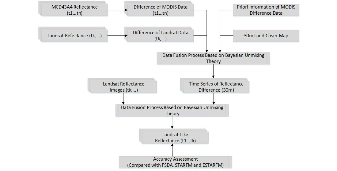
2.1.1. Study Area of Huailai

To test our algorithm, we conducted the first experiment over a small area in Huailai County, Hebei Province, China, located around the experimental station of the Institute of Remote Sensing and Digital Earth, Chinese Academy of Sciences (40°21′ north (N), 115°47′ east (E); Figure 1). The remote sensing image covering this area was 608 × 512 Landsat pixels, and this study area mainly consisted of forests, grass, farmland, and shrub (Figure 1).

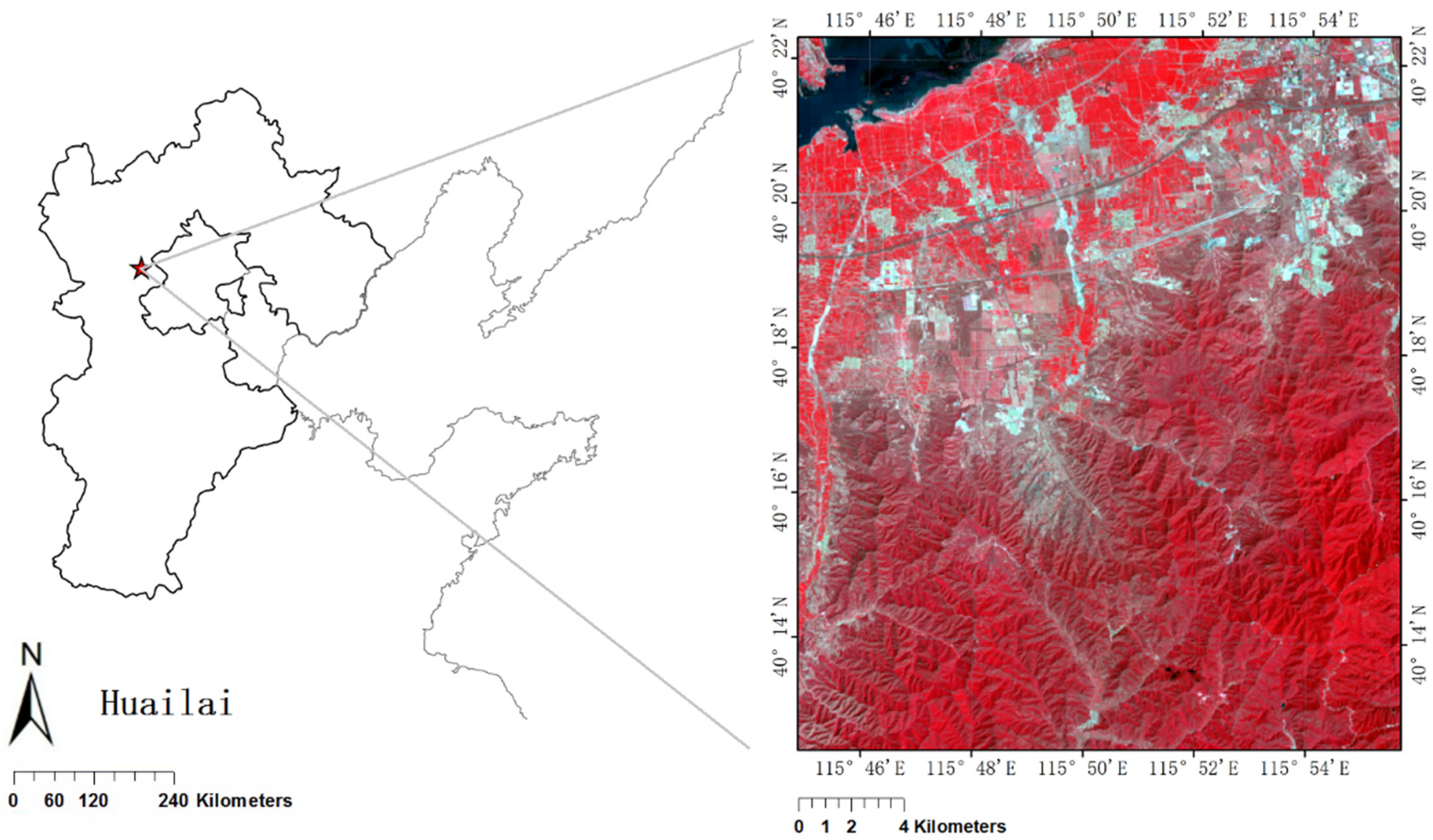
2.1.2. Study Area in Hebei

To verify the global performance, experiments were conducted in the northwest of Hebei Province (Figure 2). We chose a Landsat tile (WRS (Worldwide Reference System) -2 path 124 and row 31) as the larger area. The tile was 7582 × 7827 pixels in size at a 30 m scale, its typical elevation was approximately 480 m, and the area had a temperate continental climate. The study area was mainly made up of forests, farmland predominantly planted with corn, and grass.

2.2. Data and Processing

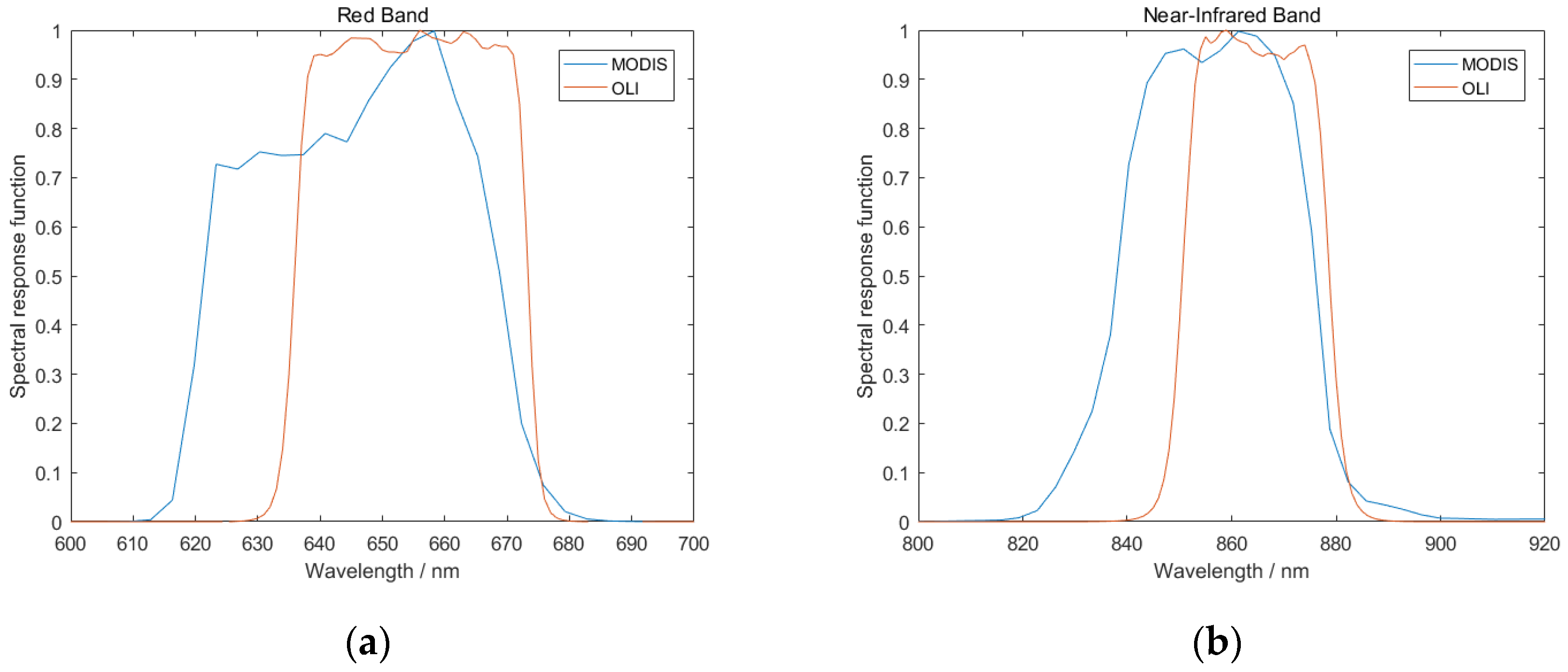
2.2.1. Data Preparation

The 30 m spatial resolution Landsat 8/OLI land surface reflectance product was downloaded from the United States Geological Survey website. This product is atmospherically corrected by the L8SR program [25,26]. We collected six images for Landsat from 2014 (DOY (Day of Year) = 94, 206, 238, 270, 286, and 318). Among them, DOY 94 and 238 were one image pair as the model input, and DOY 206 was a model verification of this pair of images. Similarly, DOY 270 and 318 represented another image pair, and DOY 286 was a verification (Figure 3).

The MCD43A4 NBAR (Nadir Bidirectional Reflectance Distribution Function (BRDF) Adjusted Reflectance) product is composed of land surface reflectance in the zenith direction, which is produced using MODIS data and adjusted using BRDF. The solar zenith angle used by each NBAR product is the median value of the solar zenith angle corresponding to the 16 day cumulative observation. Since the reflectance of all pixels is adjusted to the observation in the zenith direction, the effect of viewing angle on reflectance is eliminated, and the resulting product is more stable and consistent. MCD43A4 provides 500 m resolution data products for the first to seventh bands [27]. We collected all the MCD43A4 data from 2010 to 2014, and there were 46 images in each year.

In addition, we obtained land-cover data for these two areas for both Landsat and MODIS. The Landsat land-cover dataset was from the 1:100,000 land-use vector map in 2010 provided by the Institute of Remote Sensing and Digital Earth, Chinese Academy of Sciences, and we rasterized it into 30 m spatial resolution images [28]. We also used MCD12Q1 Land_Cover_Type_5 acquired in 2010 to identify the land-cover type for each MODIS pixel. All MODIS data were obtained from the Land Processes Distributed Active Archive Center (LP DAAC) [29].

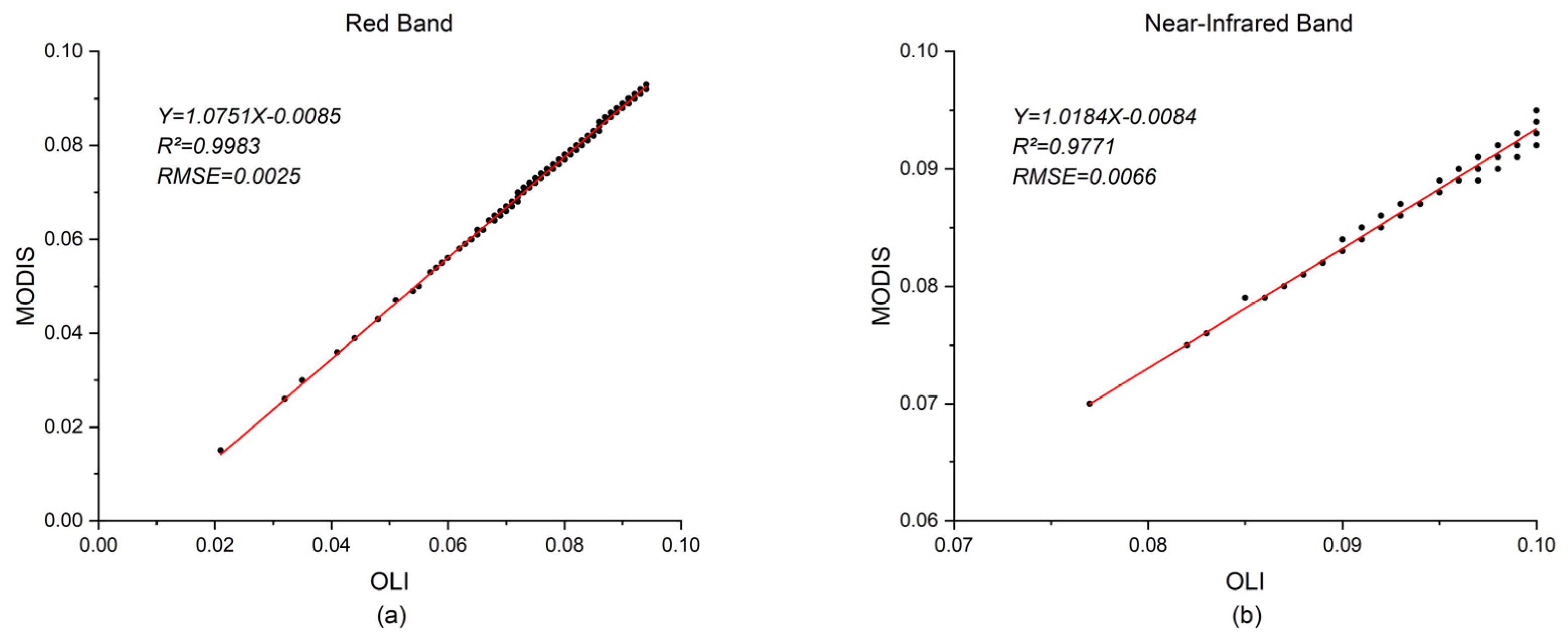
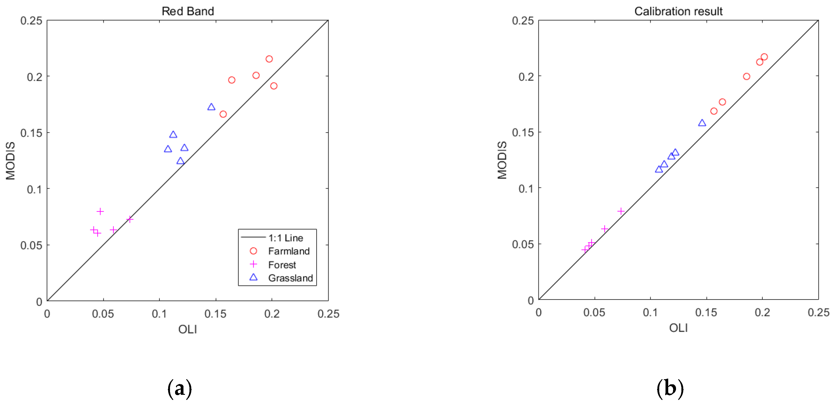
2.2.2. Data Preprocessing

(1) Reprojection and Resampling

To make the datasets consistent, they were all re-projected and geometrically registered. The MODIS MCD43A4 and MCD12Q1 products with 500 m spatial resolution were in the Integerized Sinusoidal projection; hence, we used MRT (MODIS Reprojection Tools) [30] to convert MODIS data to the same projection as Landsat data (UTM (Universal Transverse Mercator) WGS84). For convenience of calculation, all MODIS data were resampled to a spatial resolution of 480 m [17,18]. It should be noted that this process caused some data loss, which is inevitable in many current data fusion models. Generally speaking, this error has little effect on the fusion result [15,16]; thus, we ignored it.

(2) Spectral Standardization

Differences in the spectral response function of the sensor, transit time, and shooting angle meant that, even though the observation was the same object on the surface, the land surface reflectance data were not consistent. Therefore, we performed standardized processing on the multi-source data so that the parameters for each sensor used the same reference. Because the sensors have different applications, the wavelength settings were also different (Figure 4). The figure on the left (Figure 4a) compares the spectral response functions of the two sensors for the red band. The figure on the right (Figure 4b) compares the spectral response functions of the near-infrared band. The blue curve represents the MODIS sensor, and the red curve represents the Landsat OLI sensor. There were some differences between the spectral response functions of the two sensors in the same band. Therefore, we normalized the spectral response function between sensors [16].

The 6S radiation transmission model was used to simulate land surface reflectance, and the spectral response functions between the sensors were normalized to each other. In the 6S model, the input parameters of the simulation were set as follows: the sun incidence angle and the observation zenith angle ranged from 0–50° with a step size of 5°, the atmospheric mode was mid-latitude summer, the aerosol mode was continental aerosol, the aerosol optical thickness at 550 nm ranged from 0–0.6 with a step size of 0.1, and the surface reflectance ranged from 0–0.6 with a step size of 0.05. We used these parameters in the 6S model to simulate reflectance curves for the two bands, each with a different spectral response function. The simulation results of the spectral response functions of the red and near-infrared bands of MODIS and Landsat OLI data showed good agreement between the two different satellite sensors, especially for the red band (Figure 5). There was a slight deviation from the 1:1 line between the two sensors in the near-infrared band, but they were still very consistent.

According to the spectral response function of MODIS data, the spectral response function of Landsat OLI was corrected using the following formula:

$$r_{MODIS}=a\ast r_{OLI}+b,$$

(1)

where $a$ and $b$ are the slope and intercept of the fitting parameters of the simulation results between the two sensors, $r_{OLI}$ is the land surface reflectance of the Landsat data, and $r_{MODIS}$ is the land surface reflectance of the corresponding MODIS data.

By using the 6S model to process differences between the spectral response functions, we normalized the reflectance data obtained by each sensor so that it could be processed against the same benchmark. To compare the correction results, we compared the same land-cover types for both MODIS and Landsat OLI in the red and near-infrared bands. The two images were taken on the same day, and the same type of land surface reflectance at a given coordinate position was extracted and compared. Scatter diagrams for the comparison results show that the observation results of the two sensors were consistent with each other after calibration (Figure 6).

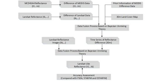
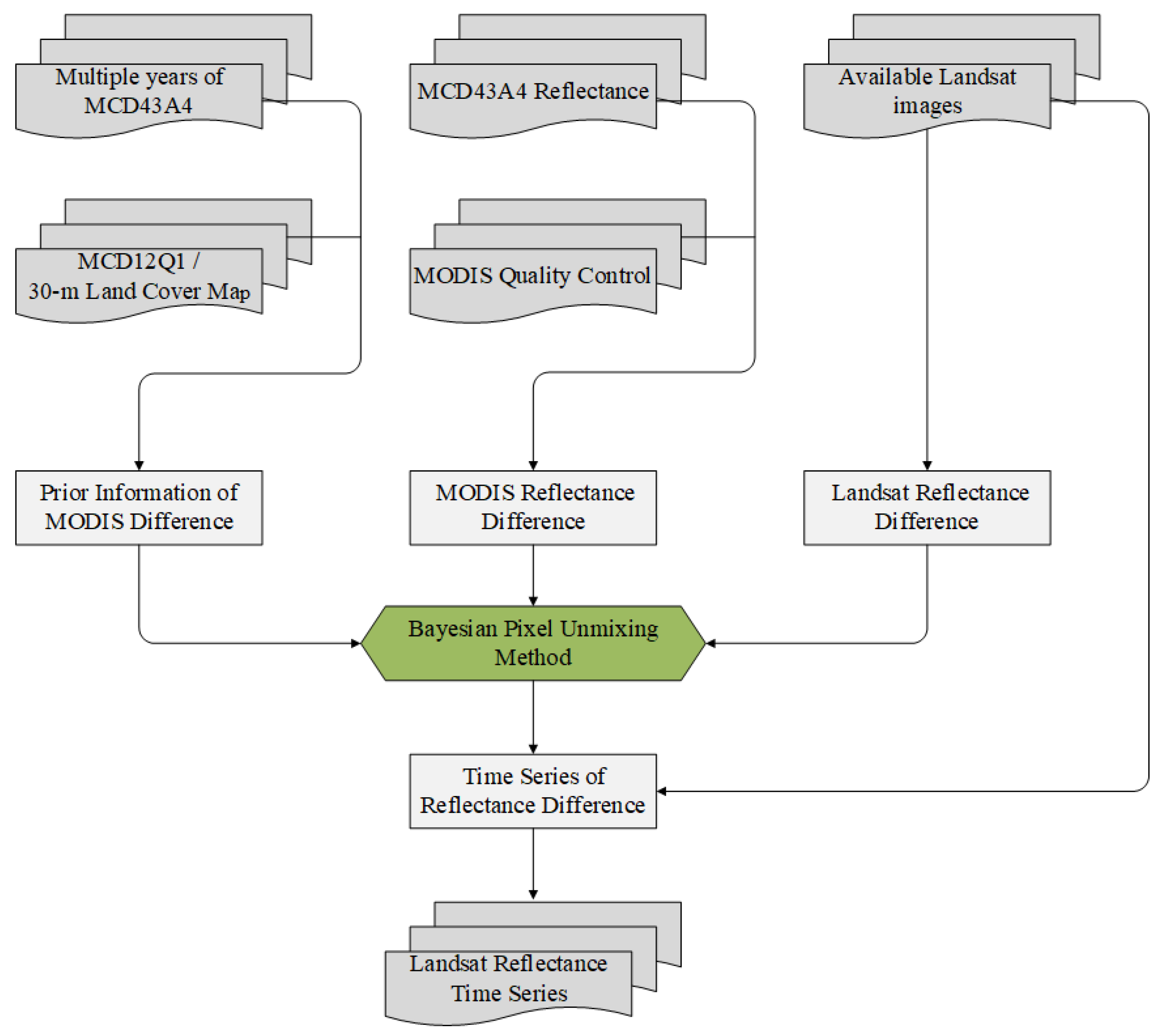
2.3. Ref-BSFM Method

This research was divided into two parts: the construction of the difference in reflectance at adjacent times, and the use of Bayesian pixel unmixing to produce high-spatial and high-temporal-resolution reflectance datasets. We first calculated the differences between 46 MCD43A4 images at adjacent times to get images of the change in reflectance. Then, we used a linear regression equation and a residual distribution model to estimate changes in the Landsat image during the next 8 days. These two sets of data were simultaneously used as inputs to the data fusion model. Afterward, to obtain images with high spatial and temporal resolution, we used the MCD43A4 product from 2010 to 2014 to construct prior information about reflectance changes in the study area. The Bayesian pixel unmixing model was used to downscale the MODIS reflectance data. Lastly, we produced Landsat-like reflectance datasets using a prediction model. Figure 7 shows a flowchart that illustrates the method we used, while the main implementation steps are described in detail in the next few sections.

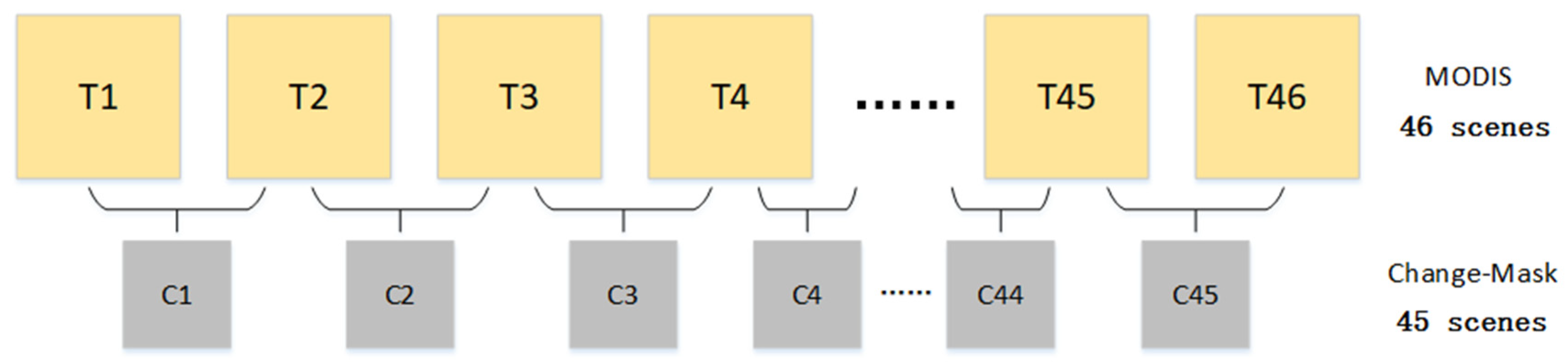
2.3.1. MODIS Data Temporal Change Detection

The construction of difference data includes two steps. We calculated the differences between MODIS data at adjacent time periods, because, in a long time series, fine-resolution remote sensing data from Landsat were scarce, and much of the change information came from MODIS data. For example, we obtained 46 scenes in a single year for the MODIS MCD43A4 product, and then we determined the change (difference) between temporally adjacent scenes to generate 45 change-mask files. The change information was stored in these change-mask files, which were numbered C1–C45, as shown in Figure 8. We then needed to construct the same change difference between adjacent times for Landsat data to provide the necessary spatial detail for the fusion results.

In reality, Landsat data with good quality available in a single year are very rare, and its 16 day revisit cycle differs from MODIS data with an 8 day temporal resolution. Therefore, the key to the Ref-BSFM method is to use the change information contained in the MODIS change-mask files to estimate the change in Landsat data over the next 8 days.

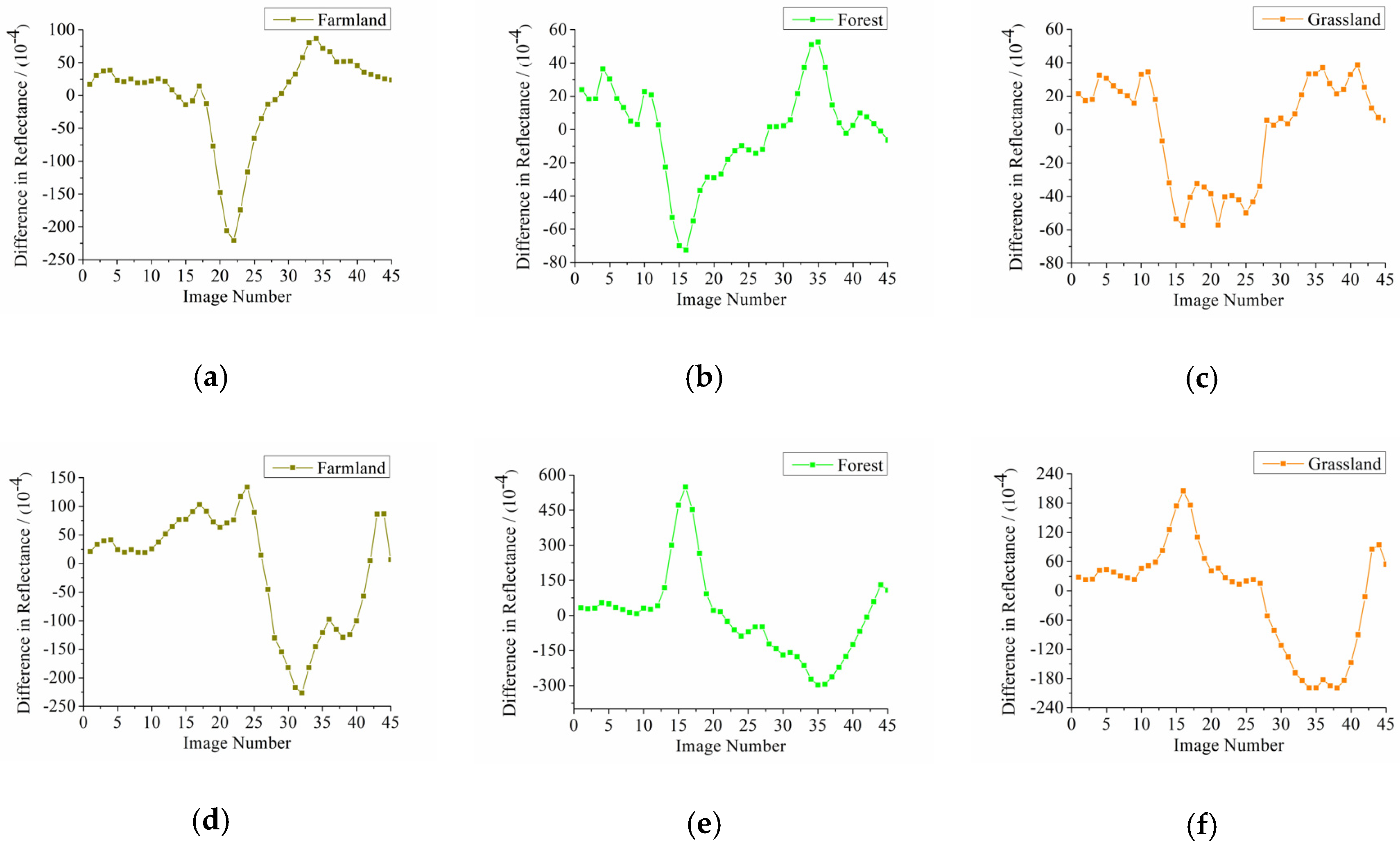
2.3.2. Building the Difference of Landsat Data

Suppose there is a pair consisting of a fine-resolution image and a coarse-resolution image with good quality during time period t1 and another coarse-resolution image for the following time period t2 (8 days later). These two adjacent coarse-resolution images can be used to estimate the change that would have occurred for the fine-resolution image at t2. We resampled all MODIS data to the same 30 m spatial resolution as the Landsat data. We used these data to build a linear regression relationship (Equation (2)) between MODIS data and Landsat data at t1. This linear model was applied to the adjacent time t2 to estimate the Landsat data at this time (Equation (3)). Note that this prediction result only retains change information from the MODIS data and does not contain the detailed spatial information from the Landsat image.

$$F_1\left(x_{ij},y_{ij},\lambda \right)=p\ast C_1\left(x_{ij},y_{ij},\lambda \right)+\mathrm{q},$$

(2)

$$F_2^S\left(x_{ij},y_{ij},\lambda \right)=p\ast C_2\left(x_{ij},y_{ij},\lambda \right)+\mathrm{q},$$

(3)

where $F_1\left(x_{ij},y_{ij},\lambda \right)$ is the Landsat image at t1, $C_1\left(x_{ij},y_{ij},\lambda \right)$ is the MODIS image after resampling at t1, $C_2\left(x_{ij},y_{ij},\lambda \right)$ is the MODIS image after resampling at t2, $F_2^S\left(x_{ij},y_{ij},\lambda \right)$ is the spatial prediction of the fine-resolution image at t2, and $p$ and $\mathrm{q}$ represent fitting coefficients for band $\lambda$ at t1, a obtained from the linear regression equation.

A high-precision land-cover map was used to get the fraction of each class (land-cover type) in a single coarse pixel. We calculated the class fractions for each coarse pixel by counting the number of fine pixels of each class using the following equation:

$$f_c\left(x_i,y_i\right)=\frac{N_c\left(x_i,y_i\right)}{m},$$

(4)

where $N_c\left(x_i,y_i\right)$ is the number of fine pixels belonging to class c within the coarse pixel at $\left(x_i,y_i\right)$. We assumed that the land-cover type did not change over a short period of time, and that the reflectance changes of the same type were also consistent.

For band $\lambda$, the temporal change of the coarse pixel at $\left(x_i,y_i\right)$ was calculated as follows:

$$\Delta \mathrm{C}\left(x_i,y_i,\lambda \right)=C_2\left(x_i,y_i,\lambda \right)-C_1\left(x_i,y_i,\lambda \right).$$

(5)

According to spectral linear mixing theory, the temporal change of a coarse pixel is the weighted sum of the temporal change of all classes within it.

$$\Delta \mathrm{C}\left(x_i,y_i,\lambda \right)={\displaystyle \sum }_{c=1}^l f_c\left(x_i,y_i\right)\times \Delta \mathrm{F}\left(\mathrm{c},\mathsf{\lambda }\right),$$

(6)

where $l$ is the number of classes, $f_c\left(x_i,y_i\right)$ is obtained from a land-cover map, and $\Delta \mathrm{F}\left(\mathrm{c},\mathsf{\lambda }\right)$ represents changes in each class, obtained using Equation (6). The fine-resolution image at t2 can be estimated as

$$F_2^T\left(x_{ij},y_{ij},\lambda \right)=F_1\left(x_{ij},y_{ij},\lambda \right)+\Delta \mathrm{F}\left(\mathrm{c},\mathsf{\lambda }\right),$$

(7)

where $F_2^T\left(x_{ij},y_{ij},\lambda \right)$ represents the temporal prediction of the fine-resolution image at t2, and $F_1\left(x_{ij},y_{ij},\lambda \right)$ represents the fine-resolution image at t1. However, the information for the fine-resolution image obtained at time t2 comes only from MODIS data; it still lacks detailed spatial information. We needed to provide it with the detailed spatial information from the Landsat image at t1.

Considering that the land-cover type might have changed or there may be within-class changes during the period from t1 to t2, we introduced the following residual system to correct for this:

$$R(x_i,y_i,\lambda )=\Delta \mathrm{C}\left(x_i,y_i,\lambda \right)-\frac{1}{m}\left[{\sum }_{j=1}^m{F}_2^T\left(x_{ij},y_{ij},\lambda \right)-{\sum }_{j=1}^m{F}_1\left(x_{ij},y_{ij},\lambda \right)\right].$$

(8)

Both $F_2^S\left(x_{ij},y_{ij},\lambda \right)$ and $F_2^T\left(x_{ij},y_{ij},\lambda \right)$ are the predictions of fine-resolution images at time t2, and we assumed that $F_2^S\left(x_{ij},y_{ij},\lambda \right)$ is closer to the real image at t2 than $F_2^T\left(x_{ij},y_{ij},\lambda \right)$, because $F_2^S\left(x_{ij},y_{ij},\lambda \right)$ contains both the information from the fine-resolution image at t1 and the change information obtained from the MODIS data [17]. The error for the prediction of $F_2^T\left(x_{ij},y_{ij},\lambda \right)$ was then estimated as

$$\mathrm{E}\left(x_{ij},y_{ij},\lambda \right)=F_2^S\left(x_{ij},y_{ij},\lambda \right)-F_2^T\left(x_{ij},y_{ij},\lambda \right).$$

(9)

Both Equations (8) and (9) represent errors when predicting the fine-resolution image at t2. We then introduced a weight distribution coefficient to guide the distribution of these two errors. This concept comes from the FSDAF data fusion model published by Zhu in 2016 [17].

$$\mathrm{I}\left(x_{ij},y_{ij},\lambda \right)=({\displaystyle \sum }_{k=1}^m{I}_k)/m,$$

(10)

where $I_k$ = 1 when the k-th fine pixels within a moving window (its size is one coarse pixel) have the same land-cover type as the central fine pixel $\left(x_{ij},y_{ij}\right)$; otherwise, $I_k$ = 0. The weight for combining the two errors through $\mathrm{I}\left(x_{ij},y_{ij},\lambda \right)$ is

$$\mathsf{\omega }\left(x_{ij},y_{ij},\lambda \right)=\mathrm{E}\left(x_{ij},y_{ij},\lambda \right)\times \mathrm{I}\left(x_{ij},y_{ij},\lambda \right)+R(x_i,y_i,\lambda )\times \left[1-\mathrm{I}\left(x_{ij},y_{ij},\lambda \right)\right].$$

(11)

The weight is then normalized as

$$\mathrm{W}\left(x_{ij},y_{ij},\lambda \right)=\frac{\mathsf{\omega }\left(x_{ij},y_{ij},\lambda \right)}{{\sum }_{j=1}^m\mathsf{\omega }\left(x_{ij},y_{ij},\lambda \right)}.$$

(12)

Lastly, when $\left(x_{ij},y_{ij}\right)$ belongs to class c, the prediction of the total change within a fine pixel between t1 and t2 is

$$\Delta \mathrm{F}\left(x_{ij},y_{ij},\lambda \right)=m\times R(x_i,y_i,\lambda )\times \mathrm{W}\left(x_{ij},y_{ij},\lambda \right)+\Delta \mathrm{F}\left(\mathrm{c},\mathsf{\lambda }\right).$$

(13)

In fact, we added $F_1\left(x_{ij},y_{ij},\lambda \right)$ and $\Delta \mathrm{F}\left(x_{ij},y_{ij},\lambda \right)$ to directly and accurately predict fine-resolution image data at time t2. This calculation is limited to adjacent time periods. The use of a linear correlation model between images is only accurate when the images used in prediction images are close in time. We proved through a large number of experiments that, when the time span is too long, continuing to use the same linear model would lead to large errors in the results. Therefore, we chose to construct difference data for adjacent times, expecting that more images could be predicted in this manner.

2.3.3. Obtaining Prior Information

It is known that the trends in reflectance time-series data for a specific land-cover type are relatively stable over several years and, thus, reflectance trend information in a time series for each land-cover type summarized from data for many years can be utilized as prior information. In this study, there were 46 reflectance observations for each land-use type for a year (Figure 9). We calculated the average value of reflectance changes for each land-cover type over a 5 year period and obtained the difference between adjacent time periods, in turn creating 45 difference values for each land-cover type in a given year (Figure 10). The prior information was used as input data for the next stage.

We used a 30 m fine-resolution land-cover map and 480 m coarse-resolution MCD12Q1 land-cover product to identify MODIS “pure” pixels. For example, we spatially overlapped the 30 m land-cover map and the MDC12Q1 product. If a coarse-resolution pixel was flagged with the land-cover type “grass” in the MCD12Q1, and more than 90% of the 30 m resolution pixels were also flagged with the type “grass” in this coarse pixel, we regarded this MODIS pixel as a “pure” pixel. The MCD43A4 reflectance dataset and its QA quality control dataset from 2010 to 2014 were then used to calculate extremely precise average reflectance for the study area, and a multi-year average reflectance time series was established for each land-cover type. Lastly, we used the Savitzky–Golay (S–G) filtering algorithm to optimize the time series curve and calculated the difference between two adjacent times to obtain the final prior information. At the beginning and end of each year, observed reflectance values might be high due to snow cover and other issues. In this study, we used MODIS snow-cover products to eliminate abnormal values and used data from the same time period from years without snow coverage to replace them. This resulted in a reflectance curve that was more realistic. Note that, when we used the a priori information for these corrected time period data, we gave them greater uncertainty (i.e., greater variance).

2.3.4. Bayesian Pixel Unmixing

The unmixing process used in this study was the Bayesian pixel unmixing process developed for the NDVI-BSFM data fusion method [18]. In the NDVI-BSFM model, the inputs are the original NDVI prior information and observation data, while, in the Ref-BSFM model, the inputs are the prior information of the reflectance difference between adjacent times, as described in Section 2.3.1.

Usually, we define a sliding window of [n × n] on the MODIS image, where each pixel corresponds to a difference in MODIS reflectance and contains the area fractions for the m types of land cover. Then, in the sliding window, an area component matrix A with n × n rows and m columns can be obtained.

We treated the filtered multi-year average reflectance difference time series of pure MODIS pixels for each land-cover type as prior information and assumed it obeyed a Gaussian distribution with mean value $R_p$ and covariance matrix $\mathrm{\Sigma }\mathrm{p}$. At the same time, we assumed that the MODIS reflectance difference observations ($R_0$) in the sliding window comprised a Gaussian distribution with errors, and its covariance matrix was ${\mathrm{\Sigma }}_0$. Under these assumptions, according to the Bayesian theory and the conjugate of the Gaussian distribution, the posterior distribution also obeys a Gaussian distribution with expectation value ${\mathsf{\mu }}_e$ and covariance matrix $\mathrm{\Sigma }\mathrm{e}$.

$$\mathrm{\Sigma }\mathrm{e}=\left[{\mathrm{\Sigma }\mathrm{p}}^{-1}+A^T{\mathrm{\Sigma }}_0{}^{-1}\mathrm{A}\right]{ }^{-1},$$

(14)

$${\mathsf{\mu }}_e=\mathrm{\Sigma }\mathrm{e}\times \left[A^T{\mathrm{\Sigma }}_0{}^{-1}{R}_0+{\mathrm{\Sigma }\mathrm{p}}^{-1}{R}_p\right]{ }^{-1},$$

(15)

where A represents the area fraction of each land-cover type in this sliding window, and ${\mathsf{\mu }}_e$ is the expected value of the posterior probability, which is the estimated value of the minimum mean square error for each end member.$\mathrm{\Sigma }\mathrm{p}$ and ${\mathrm{\Sigma }}_0$ are empirical values, which are different in different areas. For example, according to a large amount of data processing experience, when data quality is relatively good,$\mathrm{\Sigma }\mathrm{p}$ is defined as 20 and ${\mathrm{\Sigma }}_0$ is defined as 40, providing good results. When the MODIS observation data quality is poor, the value of ${\mathrm{\Sigma }}_0$ needs to be increased (usually, we define it as 200), because we used the value of the a priori information to replace the MODIS observations of poor quality. Actually, we found through sensitivity analysis of these parameters that the individual values of ${\mathrm{\Sigma }}_0$ and $\mathrm{\Sigma }\mathrm{p}$ are not remarkable, but the ratio $\mathrm{\Sigma }\mathrm{r}$ = $\mathrm{\Sigma }\mathrm{p}$/${\mathrm{\Sigma }}_0$ is the key index for controlling the relative importance of the prior information and the observations. If the MODIS observations are of poor quality, then, after reducing the $\mathrm{\Sigma }\mathrm{r}$, more stress is placed on the prior information, thereby decreasing the influence of the observation noise on the estimators, and vice versa. Therefore, better results can be obtained by optimizing $\mathrm{\Sigma }\mathrm{r}$ [18,19,20].

In this process, the sliding window was moved pixel by pixel, and a model was constructed for each pixel. Each MODIS pixel, thus, had a unique posterior probability expectation value for each land-cover type. Lastly, combined with land-use data, the MODIS data could be downscaled to 30 m.

2.3.5. Prediction of Reflectance Difference Datasets

The 30 m spatial resolution data were obtained through the unmixing process. Their spectral characteristics were derived from MODIS data, but the detailed spatial information of Landsat data was not yet available. To include that information, we established a regression relationship between the Landsat difference image and the unmixed image at t1 and tk to adjust the results of each subsequent prediction.

$$L_{t1}=p\times M_{t1}+q_{t1},$$

(16)

$$L_{tk}=p\times M_{tk}+q_{tk},$$

(17)

where $L_{t1}$ represents the Landsat difference image constructed at t1, $M_{t1}$ represents the difference image of 30 m MODIS obtained using the Bayesian unmixing method, and $p$, $q_{t1},$ and $q_{tk}$ are fitting coefficients. The coefficient $p$ is determined by the characteristics of the two sensors and atmospheric conditions. In this study, we considered that the atmospheric conditions were the same, and this coefficient did not change with time. This was determined using the image pair at t1 (Equation (16)), where $q_{t1}$ is the error term, which changes with the time period of difference. When the value of $M_{t1}$ is larger, the magnitude of the change of this coefficient is larger, indicating there is a positive correlation between $q_{t1}$ and $M_{t1}$.

$$\frac{L_{t1}-p\ast M_{t1}}{M_{t1}}=\frac{L_{tk}-p\ast M_{tk}}{M_{tk}},$$

(18)

$$L_{tk}=p\ast M_{tk}+\frac{L_{t1}-p\ast M_{t1}}{M_{t1}}\ast M_{tk}.$$

(19)

Using Equation (19), we predicted the difference images during 45 adjacent time periods during the year. These results not only had a spatial resolution of 30 m, but also had detailed spatial information from the Landsat data. At this point, the original Landsat data and these images were used to create images of predicted change in reflectance at tk. If there was more than one available Landsat observation in a year, the weight distribution and comprehensive utilization between these data improved the accuracy of the prediction.

$$L_{tk}=p\ast M_{tk}+\frac{{\sum }_{j=1}^n\omega \left(t_k,t_j\right)\ast \frac{L_{tj}-p\ast M_{tj}}{M_{tj}}\ast M_{tk}}{{\sum }_{j=1}^n\omega \left(t_k,t_j\right)},$$

(20)

where j is a variable that ranges from 1 to n,$L_{tj}$ and $M_{tj}$ are obtained on date tj, and $\omega \left(t_k,t_j\right)$ is a function of time and distance.

$$\omega \left(t_k,t_j\right)=\frac{1}{t_k-t_j}\times \frac{1}{M_{tk}-M_{tj}},$$

(21)

$$L_k=\{\begin{array}{c}{L}_1-\left(L_{t1}+L_{t1-1}+L_{t1-2}+\dots +L_{tk}\right) t_k<t_1\\ L_1+\left(L_{t1}+L_{t1+1}+L_{t1+2}+\dots +L_{tk}\right) t_k\ge t_1 \end{array},$$

(22)

where $L_1$ is the original Landsat/OLI land surface reflectance data obtained at time t1, $L_{tn}$ (n = 1, 2, …, 45) represents the difference image at time tn, and $L_k$ represents the prediction result of the fine-resolution image at time tk.

The Ref-BSFM fusion results that we developed were compared with several mainstream data fusion algorithms, namely, STARFM, ESTARFM, and FSDAF. Even with all of the current research on data fusion, a unified standard has not yet been created for an accuracy evaluation index. In this study, we summarized the most commonly used indicators that have been published to verify the advantages of the Ref-BSFM data fusion model.

We calculated six statistics between the predictions and the Landsat observations to quantify the global accuracy: the average absolute difference (AAD, Equation (23)), the average absolute relative difference (AARD, Equation (24)), the correlation coefficient (r, Equation (25)), the root-mean-square error (RMSE, Equation (26)), the structural similarity index measure (SSIM, Equation (27)), and the peak signal-to-noise ratio (PSNR, Equation (28)).

$$\mathrm{AAD}=\frac{1}{n}{{\displaystyle \sum }}_{i=1}^n\left|R_i^p-R_i^0\right|,$$

(23)

$$\mathrm{AARD}=\frac{1}{n}{{\displaystyle \sum }}_{i=1}^n|(R_i^p-R_i^0)/R_i^0|,$$

(24)

$$\mathrm{r}=\frac{{\sum }_{i=1}^n\left(R_i^p-\overline{R^p}\right)\left(R_i^0-\overline{R^0}\right)}{\sqrt{{\sum }_{i=1}^n\left(R_i^p-\overline{R^p}\right){ }^2}\ast \sqrt{{\sum }_{i=1}^n\left(R_i^0-\overline{R^0}\right){ }^2}},$$

(25)

$$\mathrm{RMSE}=\sqrt{\frac{{\sum }_{i=1}^n\left(R_i^p-R_i^0\right){ }^2}{n}},$$

(26)

$$\mathrm{SSIM}=\frac{\left(2{\mu }_x{\mu }_y+c_1\right)\left(2{\sigma }_{xy}+c_2\right)}{\left({\mu }_x^2+{\mu }_y^2+c_1\right)\left({\sigma }_x^2+{\sigma }_y^2+c_2\right)},$$

(27)

$$\mathrm{PSNR}=10\ast lo{g}_{10}\left(\frac{MA{X}_0^2}{MSE}\right),$$

(28)

where, in Equations (23)–(26), $R_i^p$ and $R_i^0$ are the predicted and observed values for pixel i, respectively, in Equation (27), μ represents the mean of the two images, σ represents the variance of the two images, and ${\sigma }_{xy}$ represents the covariance of the two images, and, in Equation (28), MSE represents the mean square error of the two images, and $MA{X}_0^2$ represents the maximum value of the pixels in the verification image.

3. Results

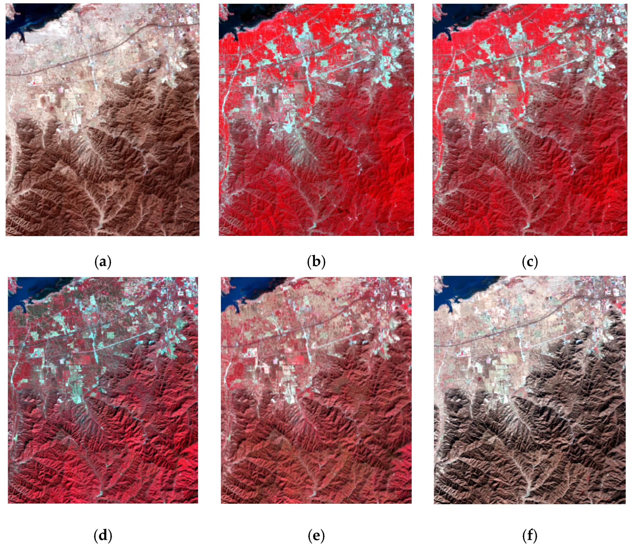
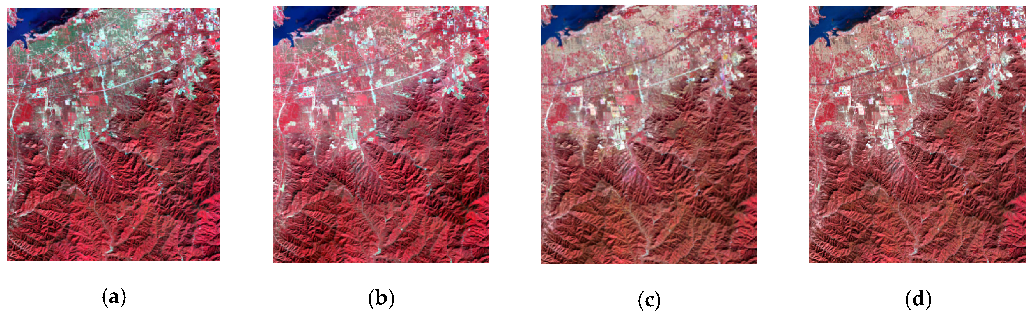
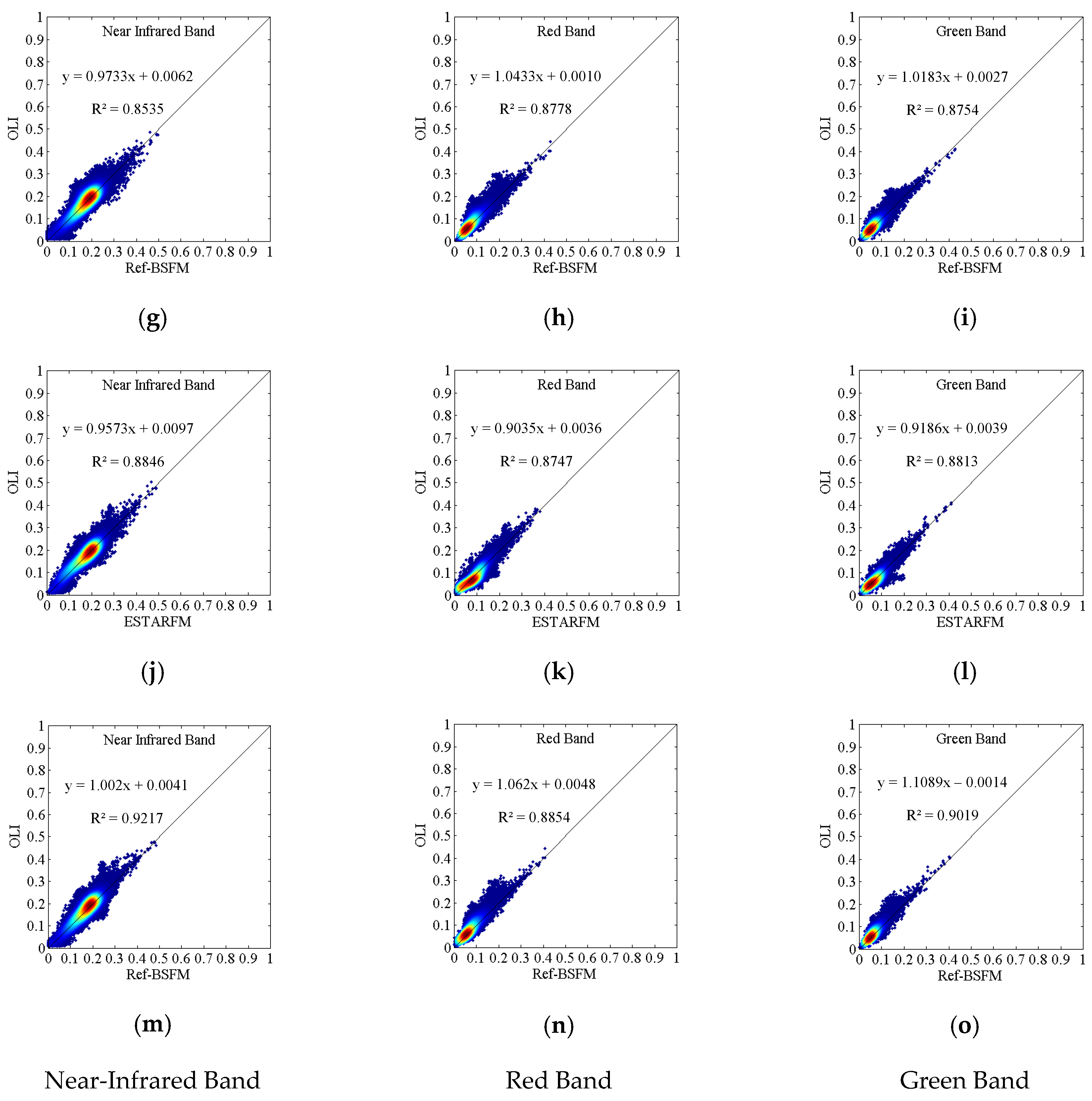
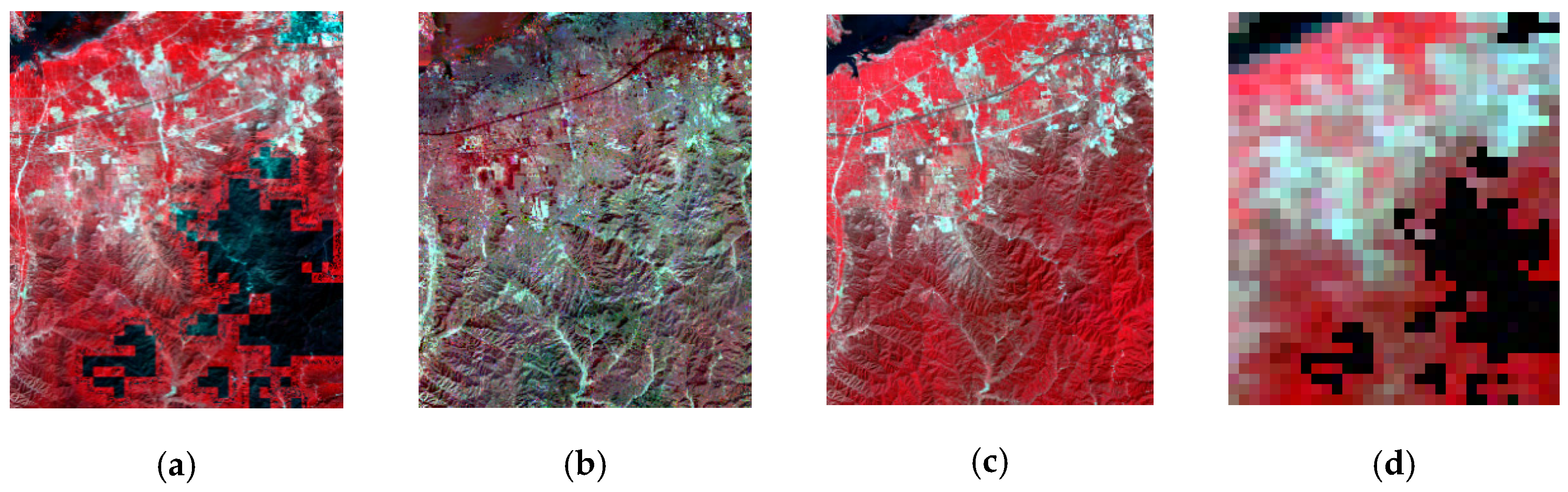
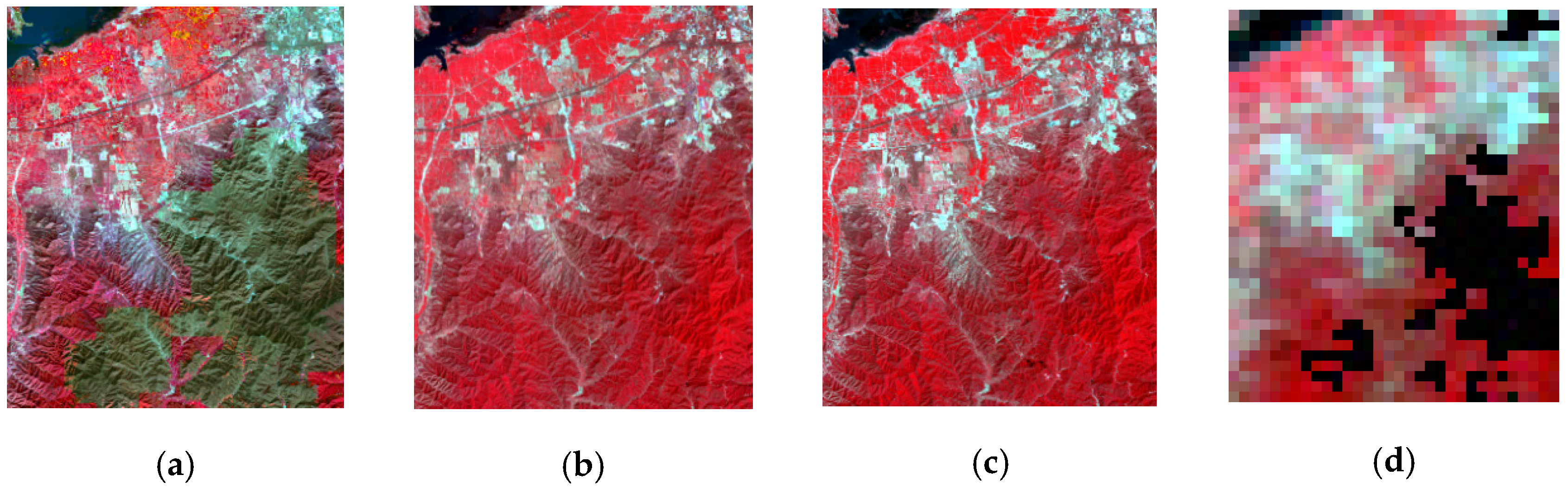
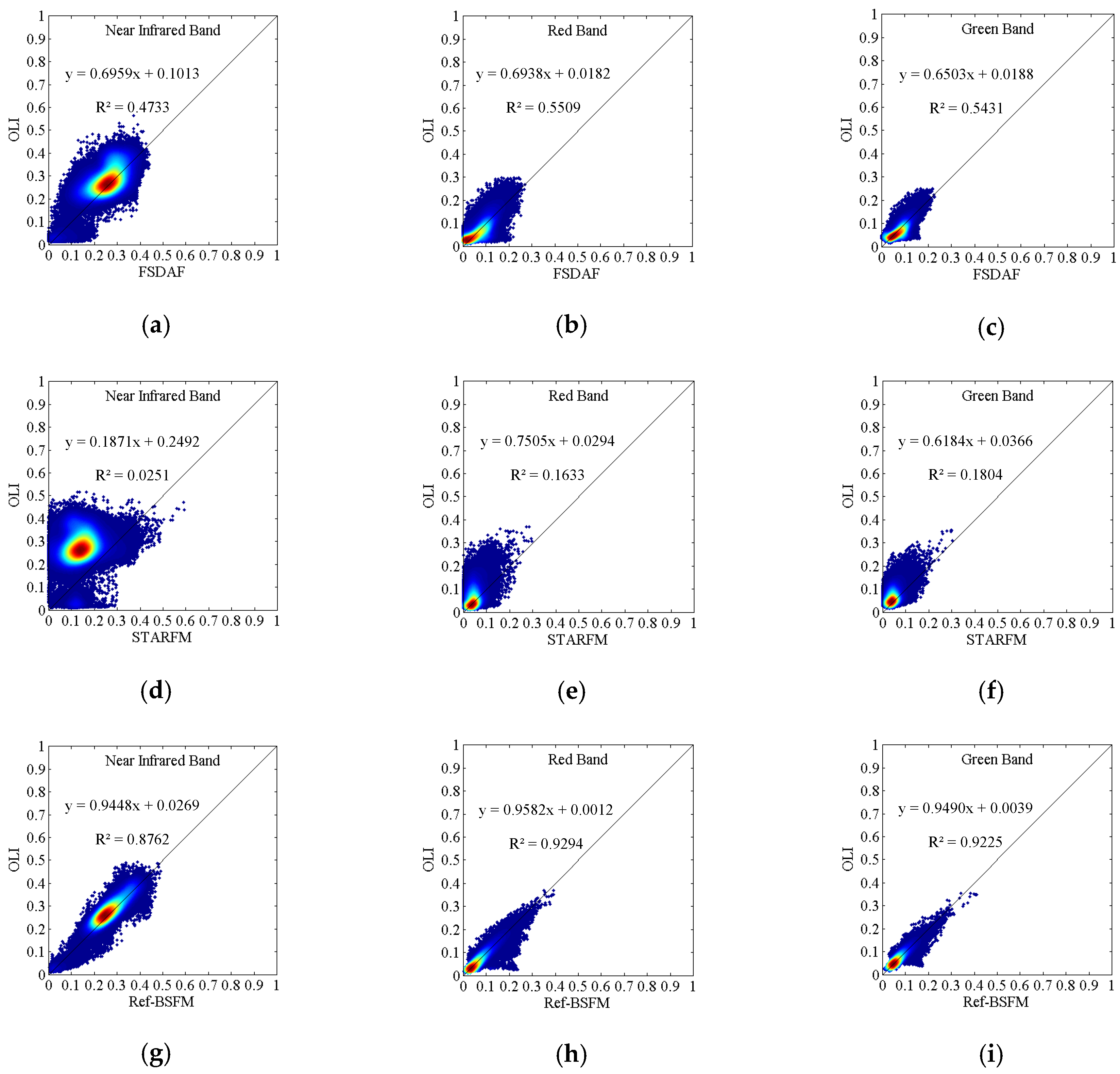
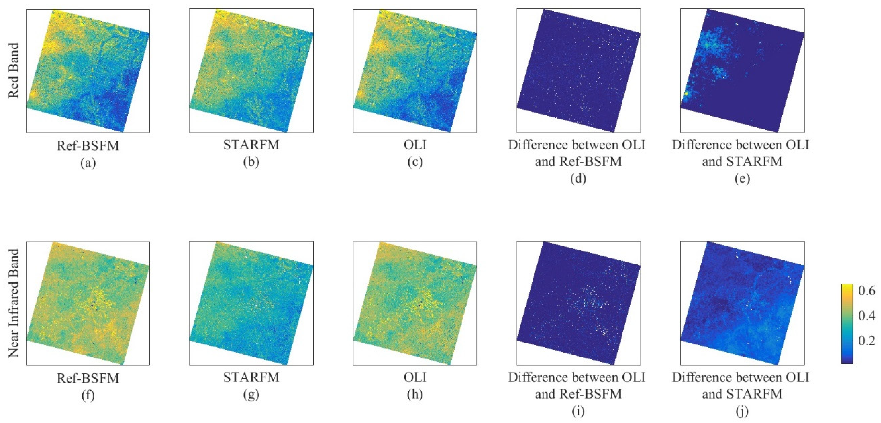
3.1. Performance Comparison over a Small Area in Huailai

The quality of MODIS data is more important to the final results; therefore, we analyzed the fusion results of the Ref-BSFM model separately for the two cases of MODIS data with good quality and poor quality. We then compared the results with other fusion models (STARFM, ESTARFM, and FSDAF). We used six Landsat 8 land surface reflectance images (DOY = 94, 206, 238, 270, 286, and 318) as inputs or verification data for the fusion model in 2014. Due to the inconsistency in transit time, a cloudless area on Landsat images may have been covered by clouds in the same area of a MODIS image.

It should be noted that FSDAF and STARFM default to inputting a pair of coarse- and fine-resolution images for prediction, while ESTARFM uses two pairs (two coarse- and two fine-resolution) of images for prediction. The Ref-BSFM supports the input of both one pair of images and multiple pairs of images. To eliminate the error caused by inputting different numbers of image pairs, we discuss the performance of the four models below using a different number of inputs.

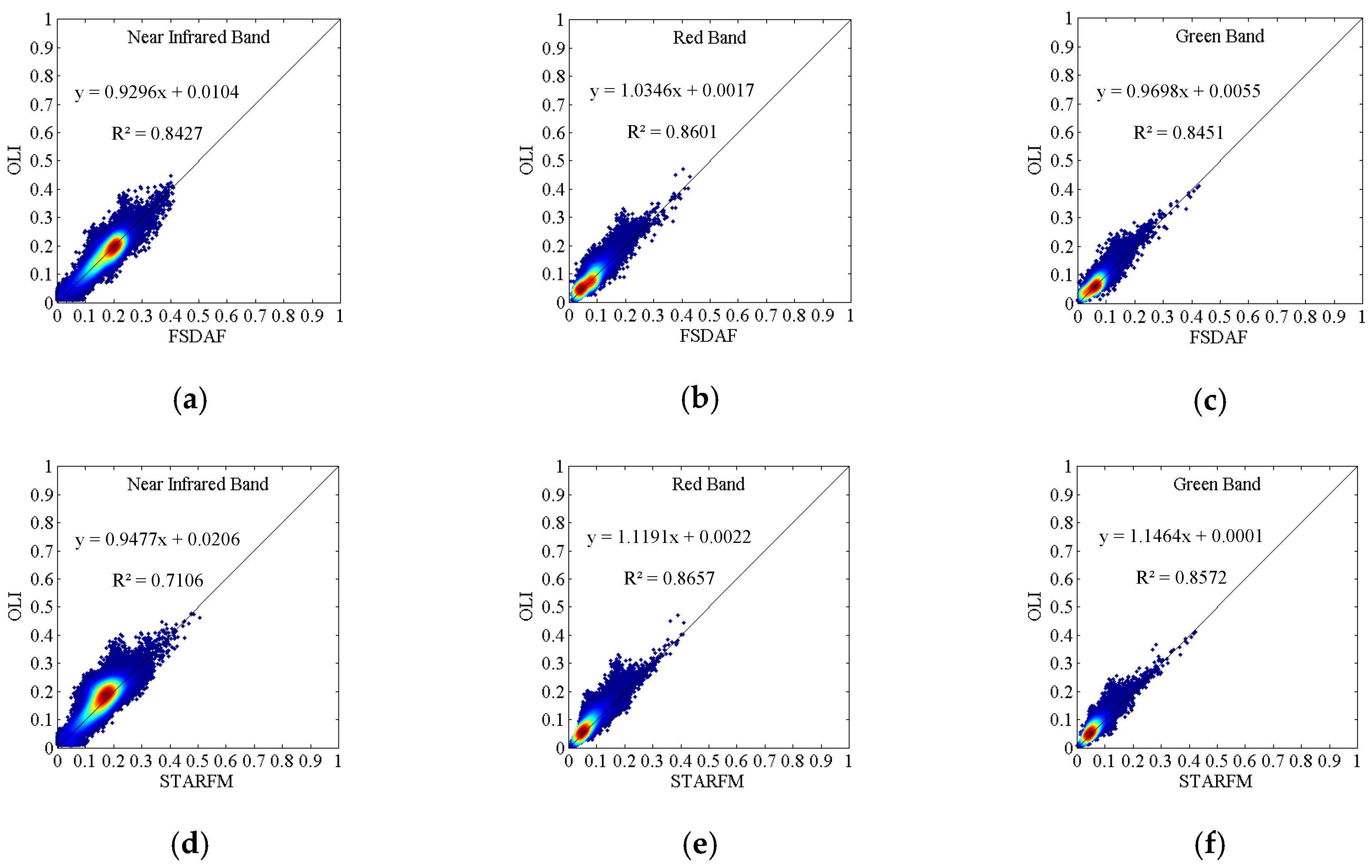
3.1.1. Performance Based on Cloudless MODIS Data

● Inputting one pair of images

A total of two Landsat and MODIS image pairs (DOY = 270 and 318) for the Huailai area were able to be used to run the Ref-BSFM fusion model, and the remaining image (DOY = 286) was used to verify the accuracy of the fusion results. We first used one Landsat and MODIS image pair (DOY = 270) for prediction (DOY = 286) and compared the prediction results of Ref-BSFM with both FSDAF and STARFM (Figure 11). At first glance, all three models generated similar results. Prediction results from FSDAF and STARFM were different from the observed values in the OLI image, while results from Ref-BSFM more closely matched the observed values. Because we used a single pair of input images, when the reflectance between the input date and the predicted date was quite different, model predictability was lower (Figure 11a,b). That is, prediction results were more similar to values at the input date, and the color of the results after the near-infrared–red–green composite was deeper.

The FSDAF first classified Landsat data at the input date; hence, the classification result greatly affected the fusion result (Figure 11a). For example, mountainous areas have many shadows; if the shadow area cannot be identified correctly, the wrong classification would lead to unrealistic outputs in the fusion result. The STARFM method produced good results, but its principle of searching for similar pixels in the neighborhood led to the loss of some detailed spatial information, which resulting in an image that looked too smooth (Figure 11b), whereas Ref-BSFM used a high-precision land-cover dataset, which could effectively deal with shadow problems in FSDAF. In addition, the search strategy of neighboring similar pixels was not used in Ref-BSFM; thus, there was no loss of spatial details. Although Ref-BSFM (Figure 11c) also used a single pair of input images, it combined many years of a priori information based on MODIS data during the time period. In other words, this additional information produced predictions closer to observed values in OLI (Figure 11d).

● Two pairs of images

We used two Landsat and MODIS image pairs (DOY = 270 and 318) to predict changes in reflectance for DOY = 286. We compared the output from Ref-BSFM to outputs from ESTARM. The ESTARFM method added a conversion coefficient, improving the ability of the STARFM method to capture spatial heterogeneity. As a result, it performed better than STARFM in terms of spatial details and image quality, and its accuracy was similar to that of Ref-BSFM (Figure 12). Both of these images closely matched the OLI image. However, it should be noted that the calculation of the ESTARM method is very time-consuming when compared with that of the Ref-BSFM method.

Increasing the number of input image pairs had the same effect as using a priori MODIS data. It compensated for the error caused by the large reflectance difference and improved the accuracy of the prediction results (Figure 12).

We used six accuracy evaluation indicators to quantitatively express the advantages of the Ref-BSFM method, as mentioned in Section 2. The overall accuracy of Ref-BSFM was higher than that of the other three methods (Figure 13 and

Table 1. Values of r, RMSE, AAD, AARD, SSIM, and PSNR between the predicted values produced using the four methods and the actual Landsat reflectance observations on DOY = 286.

	Method	Band	r	RMSE	AAD	AARD	SSIM	PSNR
Input: one pair of images	FSDAF	NIR	0.9180	0.0626	0.0877	0.6974	0.5236	38.2108
		Red	0.9274	0.0217	0.0101	0.1468	0.7477	50.1605
		Green	0.9193	0.0617	0.0842	0.6514	0.5461	39.4421
	STARFM	NIR	0.8430	0.0821	0.0210	0.5288	0.7304	22.2600
		Red	0.9304	0.0215	0.0091	0.1315	0.8005	50.1605
		Green	0.9259	0.0347	0.0141	0.1467	0.7648	48.7742
	Ref-BSFM	NIR	0.9239	0.0251	0.0142	0.1111	0.8183	44.6935
		Red	0.9369	0.0204	0.0083	0.1228	0.8052	52.3408
		Green	0.9356	0.0198	0.0097	0.1214	0.8142	50.1069
Input: two pairs of images	ESTARFM	NIR	0.9405	0.0224	0.1139	0.0818	0.8320	54.9317
		Red	0.9353	0.0217	0.0108	0.1212	0.7913	53.1247
		Green	0.9388	0.0208	0.0106	0.1193	0.8042	54.4223
	Ref-BSFM	NIR	0.9601	0.0212	0.0119	0.0722	0.8972	54.8263
		Red	0.9410	0.0176	0.0121	0.1237	0.8452	56.7885
		Green	0.9497	0.0162	0.0119	0.1200	0.8525	56.0023

). By analyzing and comparing the values of these accuracy indicators, these four methods generated good prediction results; however, when we only used one pair of images to predict reflectance changes, Ref-BSFM outperformed FSDAF and STARFM. The results were more concentrated around the 1:1 line, and the coefficients of determination were consistently the highest, ranging from 0.8535 to 0.9217. In addition, from the various accuracy evaluation indicators in Table 1, Ref-BSFM had higher correlation (r), as well as lower average error (AAD) and relative error (AARD), when compared to the OLI images. It also showed higher structural similarity (SSIM) and peak signal-to-noise ratio (PSNR), indicating better image quality. To simplify the comparison process, we show the three most commonly used bands (green, red, and near-infrared bands) as examples. The fusion accuracy of the red and green bands was significantly higher than that of the near-infrared band.

There were many sources of error in Ref-BSFM. The acquisition times of MCD43A4 and Landsat data did not match exactly, which made reflectance observations between fine-coarse resolution image pairs inconsistent. The pixel quality of MCD43A4 and the accuracy of the background field of various land-cover types also affected the fusion results. In addition, the errors in position matching pixels between MCD43A4 and Landsat, as well as land-cover changes, which were ignored, added additional uncertainty to the fusion results.

3.1.2. Performance Based on MODIS Data with Clouds

When the MODIS data were cloud-covered during either the initial time or the prediction time, Ref-BSFM continued to outperform FSDAF, STARFM, and ESTARFM. We selected a total of three image pairs for 2014 with DOY of 94, 206, and 238, and we used one Landsat image (DOY = 94) to predict the Landsat-like reflectance image at DOY 206; then, we used two image pairs (DOY = 94 and 238) to make the same prediction, which was similar to the process used in Section 3.1.1. Among these images, the MODIS image at the prediction time (DOY = 206) was mostly covered by clouds. The FSDAF, STARFM, and ESTARFM methods were unable to handle cloudy pixels in an image well. Final fusion results for Ref-BSFM, on the other hand, did not show clouds in the image (Figure 14 and Figure 15).

● One pair of images

The results of FSDAF retained cloudy areas from the MODIS data, and, although there are no obvious cloud patches in the results of STARFM, its strategy of searching through neighboring pixels made the entire image smooth, and outliers from some similar pixels were included in the calculation, leading to very low accuracy in each band. As mentioned previously, the Ref-BSFM method constrained poor-quality pixels of MODIS using prior information, such that fusion results were generally closer to actual values, and no cloud patches appeared (Figure 14).

● Two pairs of images

When we increased the number of input image pairs, ESTARFM maintained good predictability in cloudless areas, but did not accurately predict reflectance changes in cloudy areas. For the same reason as above, Ref-BSFM maintained good-quality fusion results (see Figure 15).

The scatter plots of the Ref-BSFM fusion results were more concentrated, with a determination coefficient (R²) ranging from 0.8762 to 0.9315, while RMSE, AAD, and AARD values lower than those of the other three methods. Its r, SSIM, and PSNR values were higher than those of FSDAF, STARFM, and ESTARFM methods (

Table 2. Values of r, RMSE, AAD, AARD, SSIM, and PSNR between the predicted values produced using the four methods and the actual Landsat reflectance observations on DOY = 206 in clouded areas.

	Method	Band	r	RMSE	AAD	AARD	SSIM	PSNR
Input: one pair of images	FSDAF	NIR	0.6880	0.1853	0.0620	0.7675	0.1968	13.9891
		Red	0.7422	0.1756	0.0618	0.7224	0.1410	12.4437
		Green	0.7370	0.1784	0.0618	0.7341	0.1520	12.3158
	STARFM	NIR	0.1584	0.1872	0.1503	0.6531	0.1132	21.5352
		Red	0.4041	0.1895	0.0598	0.6198	0.1680	15.1226
		Green	0.4247	0.1642	0.0502	0.5744	0.1967	18.7642
	Ref-BSFM	NIR	0.9360	0.0247	0.0200	0.0881	0.8209	45.1331
		Red	0.9641	0.0200	0.0078	0.1200	0.8483	53.7812
		Green	0.9605	0.0221	0.0143	0.1347	0.8421	50.1140
Input: two pairs of images	ESTARFM	NIR	0.5904	0.0930	0.0725	0.2708	0.3314	22.7283
		Red	0.7481	0.0283	0.0227	0.5511	0.5164	40.6181
		Green	0.4249	0.1677	0.0598	0.5679	0.2021	21.4413
	Ref-BSFM	NIR	0.9412	0.0272	0.0174	0.0733	0.8751	54.1654
		Red	0.9651	0.0165	0.0069	0.1186	0.8558	56.2208
		Green	0.9609	0.0173	0.0061	0.1243	0.8872	55.4791

). The correlation coefficient between the fusion result of Ref-BSFM and observed outputs from Landsat OLI ranged from 0.9360 to 0.9651, with a very small RMSE (approximately 0.02) in each band. The SSIM ranged from 0.8209 to 0.8751, while the PSNR ranged from 45–56, both indicating that the image quality obtained by Ref-BSFM fusion was excellent (Figure 16 and Table 2).

This clearly demonstrates the advantages of the Ref-BSFM method for prediction over cloudy areas.

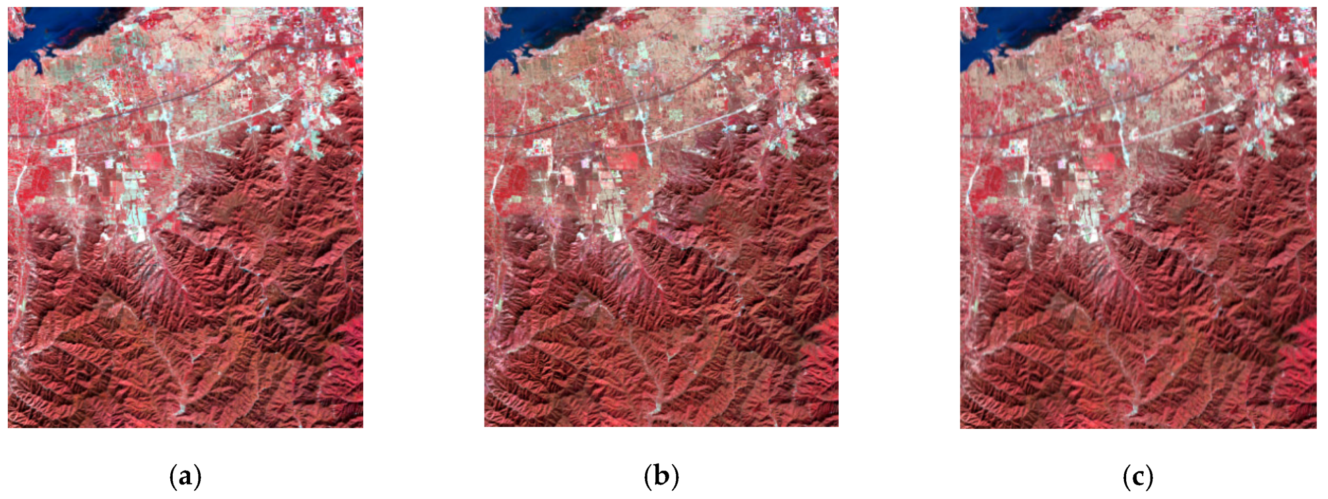
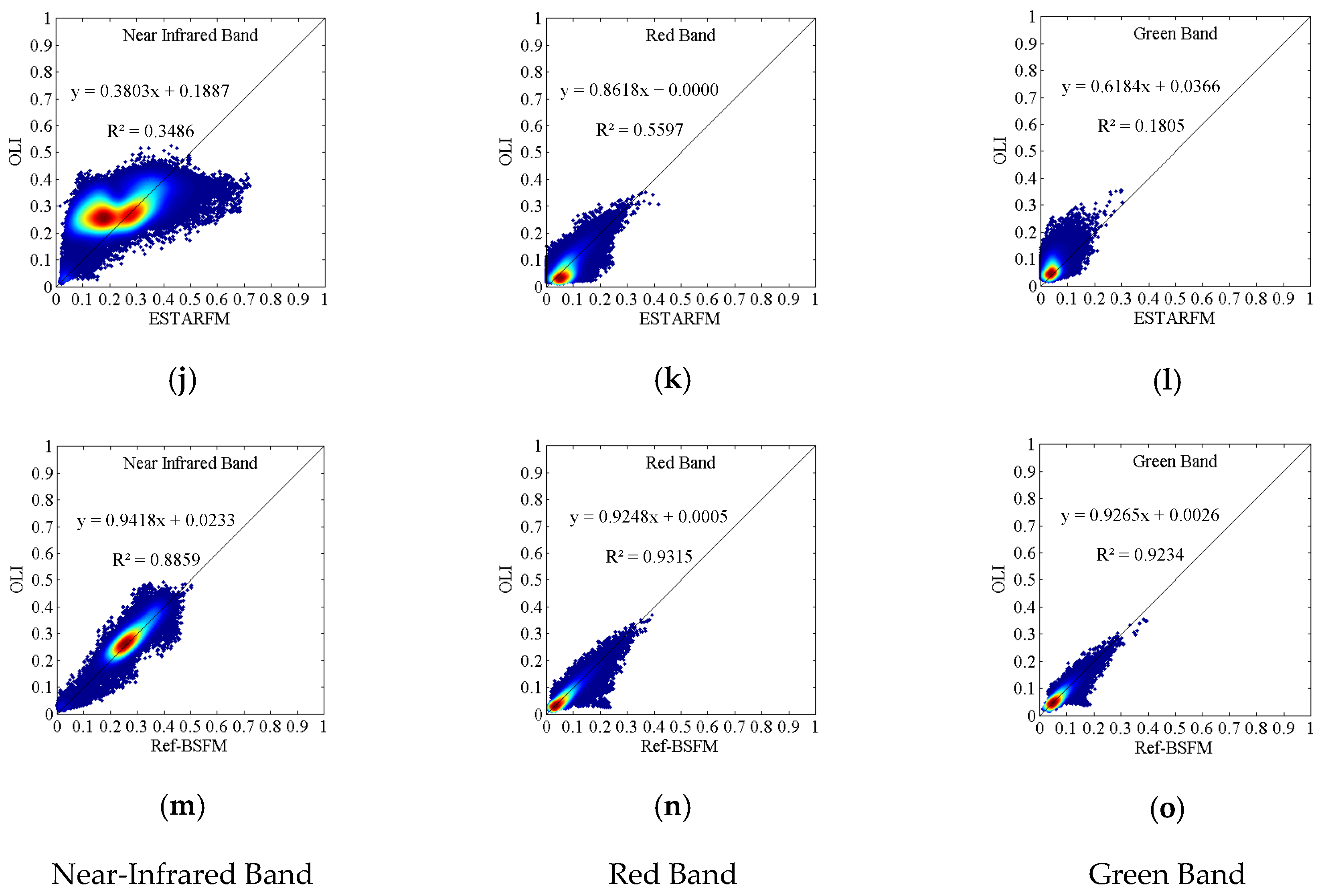
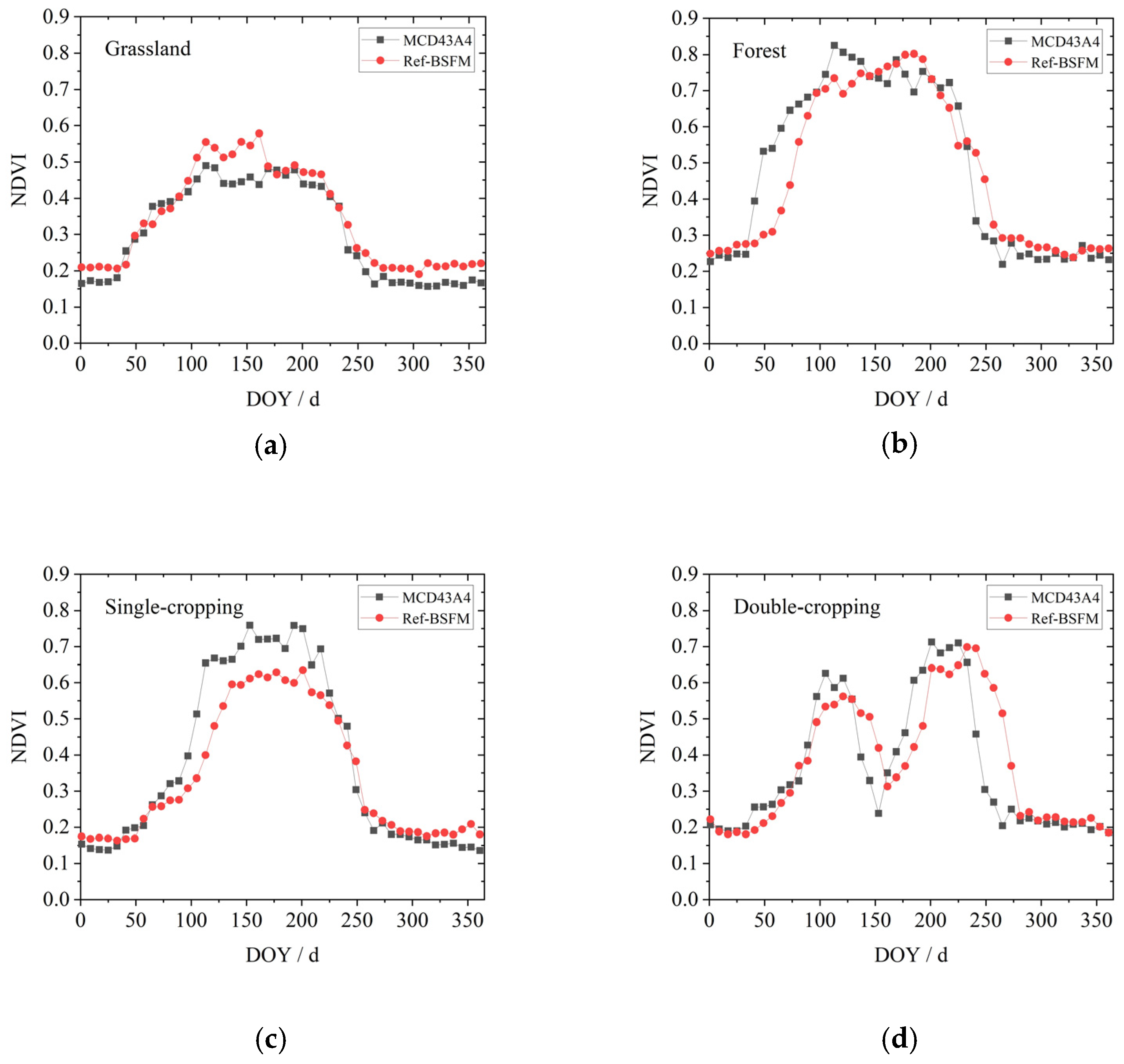
3.2. Performance Comparison over a Large Area in Hebei

We demonstrated that, in a small area, Ref-BSFM had advantages over other data fusion methods. Therefore, we applied the Ref-BSFM model to a larger study area. To avoid errors caused by an unequal number of the input image pairs, we only used one pair of fine- and coarse-resolution images for this analysis. Since the ESTARFM method typically uses two fine-resolution images and calculations for both ESTARFM and FSDAR are time-consuming over large areas, they were not included in this analysis.

In the Hebei area, we used the image pairs on DOY = 238 to predict the fine-resolution image on DOY = 286, and we compared the performance of Ref-BSFM, FSDAF, and STARFM over a large area (Figure 17 and

Table 3. Values of r, RMSE, AAD, AARD, SSIM, and PSNR between the predicted values produced using the Ref-BSFM and the STARFM methods and the actual Landsat reflectance observations on DOY = 286.

Method	Band	r	RMSE	AAD	AARD	SSIM	PSNR
Ref-BSFM	NIR	0.6972	0.0898	0.0611	0.3864	0.8533	55.0437
	Red	0.8202	0.0336	0.0203	0.3459	0.9013	65.0556
STARFM	NIR	0.6069	0.0988	0.0771	0.3768	0.8310	26.5557
	Red	0.7819	0.0337	0.0242	0.3823	0.8922	34.4263

). Figure 17a,b,f,g show the fusion performance in the red band and near-infrared band. The last two columns (Figure 17d,e,i,j) show the difference between the Landsat OLI images and the fusion images. The r and RMSE values of the fusion results of Ref-BSFM and STARFM were similar, although Ref-BSFM had a higher r and lower RMSE, showing that it was slightly more accurate than STARFM. Since the study area was large, AAD and AARD were obtained from a large amount of data; thus, their values were relatively close, and the overall accuracy of the fusion result was guaranteed to be good. In addition, both Ref-BSFM and STARFM had a structural similarity (SSIM) as high as 0.8, indicating that both of them could accurately predict the detailed spatial information, but the PSNR of the two was very different (Table 3). This indicates that Ref-BSFM had a greater advantage in maintaining overall image quality, and it was less sensitive to some outliers and can be corrected with time. Low values in the difference image of Ref-BSFM were more concentrated and values of Ref-BSFM with larger errors were more evenly distributed. There was no area with large errors in the overall image (Figure 17d,i). On the other hand, the northwest region of the red band and the southeast region of the near-infrared band of STARFM were obviously higher than that of Landsat (shown in Figure 17e,j). Combining the image quality with the statistical results in Table 3, when the study area was large, the results obtained by Ref-BSFM were closer to observed values, and the image quality was improved. In summary, Ref-BSFM had distinct advantages over other fusion methods when applied over a large area.

When Ref-BSFM was applied to a single image, it took less time to obtain the Landsat-like reflectance time series throughout the year than other methods, which is essential when applying fusion products to practical applications. When monitoring the changes in the Earth’s land surface, we usually cannot derive an accurate result from a single image; hence, we need to analyze changes over the same area across an entire year or several years, using algebraic combinations between the various bands to calculate indices that can reflect changes on the land surface, allowing the fusion products to be used to the greatest extent.

Lastly, we obtained the annual reflectance curve for Hebei and extracted the NDVI time series curves for several representative land-cover types such as forest, grassland, and farmland, comparing them with the MODIS data (Figure 18).

The NDVI curves for grassland and forest showed a single growing season, while the farmland in the Hebei area reflected the two crop cultivation methods in the region. One method involves cultivating a single crop of corn, while the other involves a double crop rotation of winter wheat and summer maize. In the fusion result of Ref-BSFM, we found pixels for both cultivation types, examining them separately. From a temporal perspective, NDVI changes for single-season crops were similar to those for grassland and forest, while the NDVI changes for double-season crops were very different. The NDVI of the entire area reached its highest value on DOY 105, and then decreased, reaching the lowest value on DOY 153. This was caused by the planting and harvesting of winter wheat. After that, due to the planting of summer maize, the NDVI gradually increased, reaching its highest value on DOY 225. Corn harvesting was basically completed on DOY 273. Using reflectance data obtained by Ref-BSFM fusion to calculate vegetation indices, we demonstrated that the results were consistent with the mature MODIS products.

4. Discussion

We found that Ref-BSFM generated good prediction results even in the presence of clouds, demonstrating that it was insensitive to outliers through its correction process of using prior information and quality control. In addition, accuracy for the images from DOY = 94, 206, and 238 was higher than that from DOY = 270, 286, and 318. Despite the existence of cloud coverage, the time span was short enough to overcome any issues. The time span of available data is the most sensitive factor among all current data fusion methods. By shortening the time span of the data as much as possible, we maximized the accuracy of the Ref-BSFM fusion method.

In fact, for many current mainstream data fusion methods based on unmixing or weight functions, a weight distribution system is adopted to reduce the influence of noise signals in the paired images as much as possible. Nevertheless, it is inevitable to have poor-quality pixels in the images. If these pixels are used in the decomposition of coarse-resolution pixels or in the calculation of similar, nearby pixels, they inevitably produce incorrect results. In Ref-BSFM, we use Bayesian theory to introduce prior information about the reflectance of various land-cover types into the decomposition process of mixed pixels. When the pixel quality of MODIS is poor, increasing the weight of the prior information greatly reduces the contribution of these poor-quality pixels to the fusion result and error transmission is reduced. For areas covered by clouds, the a priori information replaces outliers, which makes the fusion results more reasonable. In this way, this processing strategy can resolve problems with cloud coverage.

During this study, we tried many different data fusion methods for the same area to determine their performance, and we compared the resulting Ref-BSFM with current mainstream algorithms for data fusion (FSDAF, STARFM, and ESTARFM). We showed that Ref-BSFM has the following advantages: (1) Ref-BSFM maintains high prediction accuracy resulting in a high level of image accuracy and image quality, (2) it generates quality prediction results for cloudy areas, (3) when there are available Landsat data with a large time span, Ref-BSFM achieves result closer to the actual image than the results from other fusion algorithms, (4) the change information captured using MODIS data can be saved through time and fully utilized in Ref-BSFM, and (5) the NDVI-BSFM method inherits the characteristics of clear spatial details and inconspicuous patch effects. The reasons for these advantages are elaborated below.

Unlike other current mainstream data fusion methods, Ref-BSFM first constructs the difference between the two adjacent MODIS images and establishes the prior information of the difference. Because it is easy to obtain MODIS data, we can get the time-series data of MODIS for one or more years [31]. In the Ref-BSFM method, we not only use the two MODIS images at t1 and t2, but rather all of the MODIS data acquired from t1 to t2, which provides more change information for the prediction process. As long as a change could be captured by MODIS, it could be reflected in the prediction results, and the results were closer to the observed data when compared to other methods. This increased information allowed the Ref-BSFM method to obtain higher accuracy than other methods.

Similar to the NDVI-BSFM method, Ref-BSFM takes the multi-year average reflectance time series of each land-cover type as a trend and calculates the difference between adjacent time periods to construct the prior information needed. Using the framework of Bayesian unmixing [18,19,20], we combined MODIS pixel quality control datasets and made a reasonable weight assignment for the contribution of good-quality pixels and poor-quality pixels to the prediction results. If the quality of MODIS observations is too poor to reflect the true land surface state, then the prior information is given greater weight. Using this strategy, when the study area is covered by a large area of clouds, Ref-BSFM gives the prior information a greater weight to correct the value of these cloud pixels, so that the predicted results are reasonable and have low uncertainty. In this way, we combine the stability of the prior information with the validity of the observations. The traditional decomposition process of mixed pixels inevitably generates some unrealistic results [32,33,34,35], but the Bayesian theory uses prior information to constrain the decomposition values of mixed pixels; this appropriately compensates for the errors in MODIS observations, and the reflectance time series curve obtained by this method is relatively smoother. In summary, the introduction of prior information is the key to solving the cloud coverage problem for Ref-BSFM.

Ref-BSFM uses all of the coarse-resolution images from t1 to t2 to predict the fine-resolution images at t2. Although this method increases the amount of data and the complexity of the model, the prediction results have higher accuracy. Compared with FSDAF and STARFM that use only two coarse-resolution images for prediction, Ref-BSFM considers the change across the entire period from the initial time to the predicted time, and each pixel value in the Landsat-like fine resolution image is the result of contributions from all MODIS data during this period. When the interval between t1 and t2 is long, the difference in the reflectance of the coarse resolution images at these two time periods is large. There is one situation that was shown to be problematic. Assume that an image at the known time t1 has relatively sparse vegetation coverage and exhibits high land surface reflectance, while an image at predicted time t2 has lush vegetation coverage, and relatively lower land surface reflectance. When we use the images at t1 to predict the image at t2, results are closer to those of the image at time t1. That is, the fusion result is higher than the observed data [36,37,38,39,40]. The reasons for this situation are as follows: (1) using images with sparse vegetation to predict images with lush vegetation introduces great uncertainty, and (2) for the same area, MODIS has a higher reflectance value than Landsat does. We conducted a large number of experiments to aggregate Landsat images to the same spatial resolution as MODIS images, and we found that pixel values for MODIS over the same area were higher. When we unmixed the MODIS pixel at t2, the result of the unmixing was also higher, which led to final fusion results closer to the image at time t1 with sparse vegetation and high reflectance. In the Ref-BSFM method, when the time span between known time and predicted time is large, we use continuous MODIS data with an interval of 8 days, which compensates for the error caused by the large time span. This kind of data processing mechanism enables Ref-BSFM to obtain results closer to the actual images than other fusion algorithms, and the changes captured using MODIS data from t1 to t2 are saved for subsequent calculations. In other words, Ref-BSFM is more sensitive to MODIS change information. It is worth noting that Ref-BSFM can not only obtain Landsat-like reflectance images at t2, but also all Landsat-like reflectance images at an interval of 8 days from t1 to t2, which is of great significance to data production and practical applications. Methods such as FSDAF, STARFM, or ESTARFM require batch processing to produce time-series data, which is inconvenient and time-consuming [37,38]. We can also extract the reflectance curve of a pixel during this period to indirectly verify the rationality of the prediction result.

In addition, Ref-BSFM inherits many advantages of NDVI-BSFM, such as maintaining clearer spatial texture details and few MODIS patch effects [24]. However, it still has several limitations and constraints. First of all, the use of MCD43A4 data in this study excluded deviations caused by angle effects; however, as mentioned above, when the time span between the known time and the predicted is very long, predictions from Ref-BSFM are higher than the observed data for the same time, although Ref-BSFM is still more accurate than FSDAF, STARFM and ESTARFM. We have analyzed the situation and discovered that the error is caused by the data itself, which we cannot avoid [39,40]. Second, similar to the NDVI-BSFM method, some parameters in Ref-BSFM are empirical and nonautomated, such as the variance of the snow-covered area during the construction of the prior information, as well as the size of the unmixing window and the weight ratio of the prior information to the observations. Third, Ref-BSFM uses the difference between adjacent moments, which makes it necessary to pay extra attention to the accumulation of error transmissions when performing algebraic operations. Therefore, outliers in the prediction results need to be checked and manually corrected. The appearance of outliers is unavoidable in other data fusion methods, but Ref-BSFM involves more images and, thus, requires special attention. Lastly, Ref-BSFM still cannot escape the processing time required for fusing large areas, and the determination of land-cover types also affects the predicted results.

5. Conclusions

In this article, we proposed a new method for the construction of time-series Landsat-like reflectance datasets, discussing its principles and performance in detail. Ref-BSFM estimates possible changes in Landsat data during the next 8 days and calculates the difference between adjacent time periods of MCD43A4 in the same area as prior information. Together, they drive the Bayesian mixed pixel decomposition process. Lastly, a spatial information reconstruction model is used to introduce detailed spatial information into the decomposition results to obtain Landsat-like reflectance datasets with high spatial (30 m) and temporal resolution (8 days). Compared with the original NDVI-BSFM, we changed the data input form and added fitting coefficients to the reconstruction model, which more accurately expresses the relationship between Landsat and MODIS data. Ref-BSFM is more sensitive to changing information; thus, it can make more precise predictions when land-cover changes or within-class changes occur.

The reflectance datasets produced by the Ref-BSFM method can be used to construct vegetation indices or other remote sensing indices. The method responds effectively to business needs requiring high spatial resolution and temporal resolution. As such, it plays an important role in mapping land cover, monitoring dynamic surfaces, and estimating biogeochemical parameters. Moreover, the application of Ref-BSFM is not restricted to OLI and MODIS sensors. It was shown that using this method to fuse MODIS and Sentinel-2 MSI sensors images provides good results [41,42,43,44,45,46,47,48,49,50,51]; therefore, Ref-BSFM can be extended for use on a variety of remote sensing satellite platforms.

References

1. Shen, M.; Tang, Y.; Chen, J.; Zhu, X.; Zheng, Y. Influences of temperature and precipitation before the growing season on spring phenology in grasslands of the central and eastern Qinghai-Tibetan Plateau. Agric. For. Meteorol. 2011, 151, 1711–1722. [Google Scholar] [CrossRef]
2. Galford, G.L.; Mustard, J.F.; Melillo, J.; Gendrin, A.; Cerri, C.E. Wavelet analysis of MODIS time series to detect expansion and intensification of row-crop agriculture in Brazil. Remote Sens. Environ. 2008, 112, 576–587. [Google Scholar] [CrossRef]
3. Lunetta, R.S.; Knight, J.F.; Ediriwickrema, J.; Lyon, J.G.; Worthy, L.D. Land-cover change detection using multi-temporal MODIS NDVI data. Remote Sens. Environ. 2006, 105, 142–154. [Google Scholar] [CrossRef]
4. Zhu, X.; Cai, F.; Tian, J.; Williams, T.K.A. Spatiotemporal Fusion of Multisource Remote Sensing Data: Literature Survey, Taxonomy, Principles, Applications, and Future Directions. Remote Sens. 2018, 10, 527. [Google Scholar] [CrossRef] [Green Version]
5. Gorelick, N.; Hancher, M.; Dixon, M.; Ilyushchenko, S.; Thau, D.; Moore, R. Google Earth Engine: Planetary-scale geospatial analysis for everyone. Remote Sens. Environ. 2017, 202, 18–27. [Google Scholar] [CrossRef]
6. Wang, P.; Gao, F.; Masek, J.G. Operational Data Fusion Framework for Building Frequent Landsat-Like Imagery. IEEE Trans. Geosci. Remote Sens. 2014, 52, 7353–7365. [Google Scholar] [CrossRef]
7. Seto, K.C.; Fleishman, E.; Fay, J.P.; Betrus, C.J. Linking spatial patterns of bird and butterfly species richness with Landsat TM derived NDVI. Int. J. Remote Sens. 2004, 25, 4309–4324. [Google Scholar] [CrossRef]
8. Lenney, M.P.; Woodcock, C.E.; Collins, J.B.; Hamdi, H. The status of agricultural lands in Egypt: The use of multitemporal NDVI features derived from landsat TM. Remote Sens. Environ. 1996, 56, 8–20. [Google Scholar] [CrossRef]
9. Ju, J.; Roy, D. The availability of cloud-free Landsat ETM+ data over the conterminous United States and globally. Remote Sens. Environ. 2008, 112, 1196–1211. [Google Scholar] [CrossRef]
10. Asner, G.P. Cloud cover in Landsat observations of the Brazilian Amazon. Int. J. Remote Sens. 2001, 22, 3855–3862. [Google Scholar] [CrossRef]
11. Zhukov, B.; Oertel, D.; Lanzl, F.; Reinhackel, G. Unmixing-based multisensor multiresolution image fusion. IEEE Trans. Geosci. Remote Sens. 1999, 37, 1212–1226. [Google Scholar] [CrossRef]
12. Wu, M.; Niu, Z.; Wang, C.; Wu, C.; Wang, L. Use of MODIS and Landsat time series data to generate high-resolution temporal synthetic Landsat data using a spatial and temporal reflectance fusion model. J. Appl. Remote Sens. 2012, 6, 063507. [Google Scholar]
13. Wu, M.; Huang, W.; Niu, Z.; Wang, C. Generating Daily Synthetic Landsat Imagery by Combining Landsat and MODIS Data. Sensors 2015, 15, 24002–24025. [Google Scholar] [CrossRef] [Green Version]
14. Gevaert, C.M.; García-Haro, F.J. A comparison of STARFM and an unmixing-based algorithm for Landsat and MODIS data fusion. Remote Sens. Environ. 2015, 156, 34–44. [Google Scholar] [CrossRef]
15. Gao, F.; Masek, J.G.; Schwaller, M.; Hall, F. On the blending of the Landsat and MODIS surface reflectance: Predicting daily Landsat surface reflectance. IEEE Trans. Geosci. Remote Sens. 2006, 44, 2207–2218. [Google Scholar] [CrossRef]
16. Zhu, X.; Chen, J.; Gao, F.; Chen, X.; Masek, J.G. An enhanced spatial and temporal adaptive reflectance fusion model for complex heterogeneous regions. Remote Sens. Environ. 2010, 114, 2610–2623. [Google Scholar] [CrossRef]
17. Zhu, X.; Helmer, E.H.; Gao, F.; Liu, D.; Chen, J.; Lefsky, M.A. A flexible spatiotemporal method for fusing satellite images with different resolutions. Remote Sens. Environ. 2016, 172, 165–177. [Google Scholar] [CrossRef]
18. Liao, L.; Song, J.; Wang, J.; Xiao, Z.; Wang, J. Bayesian Method for Building Frequent Landsat-Like NDVI Datasets by Integrating MODIS and Landsat NDVI. Remote Sens. 2016, 8, 452. [Google Scholar] [CrossRef] [Green Version]
19. Xue, J.; Leung, Y.; Fung, T. A Bayesian Data Fusion Approach to Spatio-Temporal Fusion of Remotely Sensed Images. Remote Sens. 2017, 9, 1310. [Google Scholar] [CrossRef] [Green Version]
20. Xue, J.; Leung, Y.; Fung, T. An Unmixing-Based Bayesian Model for Spatio-Temporal Satellite Image Fusion in Heterogeneous Landscapes. Remote Sens. 2019, 11, 324. [Google Scholar] [CrossRef] [Green Version]
21. Ke, Y.; Im, J.; Park, S.; Gong, H. Downscaling of MODIS One Kilometer Evapotranspiration Using Landsat-8 Data and Machine Learning Approaches. Remote Sens. 2016, 8, 215. [Google Scholar] [CrossRef] [Green Version]
22. Song, H.; Liu, Q.; Wang, G.; Hang, R.; Huang, B. Spatiotemporal Satellite Image Fusion Using Deep Convolutional Neural Networks. IEEE J. Sel. Top. Appl. Earth Obs. Remote Sens. 2018, 11, 821–829. [Google Scholar] [CrossRef]
23. Huang, B.; Song, H. Spatiotemporal Reflectance Fusion via Sparse Representation. IEEE Trans. Geosci. Remote Sens. 2012, 50, 3707–3716. [Google Scholar] [CrossRef]
24. Moosavi, V.; Talebi, A.; Mokhtari, M.H.; Shamsi, S.R.F.; Niazi, Y. A wavelet-artificial intelligence fusion approach (WAIFA) for blending Landsat and MODIS surface temperature. Remote Sens. Environ. 2015, 169, 243–254. [Google Scholar] [CrossRef]
25. United States Geological Survey. Available online: http://earthexplorer.usgs.gov/ (accessed on 31 August 2020).
26. L8sr_Product_Guide. Available online: http://landsat.usgs.gov/documents/provisional_l8sr_product_guide.pdf (accessed on 31 August 2020).
27. Schaaf, C.B.; Gao, F.; Strahler, A.H.; Lucht, W.; Li, X.; Tsang, T.; Strugnell, N.C.; Zhang, X.; Jin, Y.; Muller, J.-P.; et al. First operational BRDF, albedo nadir reflectance products from MODIS. Remote Sens. Environ. 2002, 83, 135–148. [Google Scholar] [CrossRef] [Green Version]
28. Liu, J.; Kuang, W.; Zhang, Z.; Xu, X.; Qin, Y.; Ning, J.; Zhou, W.; Zhang, S.; Li, R.; Yan, C.; et al. Spatiotemporal characteristics, patterns, and causes of land-use changes in China since the late 1980s. J. Geogr. Sci. 2014, 24, 195–210. [Google Scholar] [CrossRef]
29. Reverb. Available online: http://reverb.echo.nasa.gov/reverb/ (accessed on 30 June 2020).
30. MODIS Reprojection Tool. Available online: https://wiki.earthdata.nasa.gov/display/DAS/ (accessed on 30 June 2020).
31. Weiss, J.L.; Gutzler, D.S.; Coonrod, J.E.; Dahm, C.N. Long-term vegetation monitoring with NDVI in a diverse semi-arid setting, central New Mexico, USA. J. Arid. Environ. 2004, 58, 249–272. [Google Scholar] [CrossRef]
32. Xin, Q.; Olofsson, P.; Zhu, Z.; Tan, B.; Woodcock, C.E. Toward near real-time monitoring of forest disturbance by fusion of MODIS and Landsat data. Remote Sens. Environ. 2013, 135, 234–247. [Google Scholar] [CrossRef]
33. Huang, B.; Zhang, H.; Song, H.; Wang, J.; Song, C. Unified fusion of remote-sensing imagery: Generating simultaneously high-resolution synthetic spatial–temporal–spectral earth observations. Remote Sens. Lett. 2013, 4, 561–569. [Google Scholar] [CrossRef]
34. Aman, A.; Randriamanantena, H.P.; Podaire, A.; Frouin, R. Upscale integration of normalized difference vegetation index: The problem of spatial heterogeneity. IEEE Trans. Geosci. Remote Sens. 1992, 30, 326–338. [Google Scholar] [CrossRef]
35. Chen, B.; Huang, B.; Xu, B. Multi-source remotely sensed data fusion for improving land cover classification. ISPRS J. Photogramm. Remote Sens. 2017, 124, 27–39. [Google Scholar] [CrossRef]
36. Emelyanova, I.V.; McVicar, T.R.; Van Niel, T.G.; Li, L.T.; Van Dijk, A.I.J.M. Assessing the accuracy of blending Landsat–MODIS surface reflectances in two landscapes with contrasting spatial and temporal dynamics: A framework for algorithm selection. Remote Sens. Environ. 2013, 133, 193–209. [Google Scholar] [CrossRef]
37. Udelhoven, T.; Schmidt, M.; Gill, T.K.; Röder, A. Long term data fusion for a dense time series analysis with MODIS and Landsat imagery in an Australian Savanna. J. Appl. Remote Sens. 2012, 6, 63512. [Google Scholar] [CrossRef]
38. Wu, M.; Huang, W.; Niu, Z.; Wang, C.; Li, W.; Yu, B. Validation of synthetic daily Landsat NDVI time series data generated by the improved spatial and temporal data fusion approach. Inf. Fusion 2018, 40, 34–44. [Google Scholar] [CrossRef]
39. Appriou, A. Uncertainty Theories and Multisensor Data Fusion; Wiley: Hoboken, NJ, USA, 2014. [Google Scholar]
40. Richardson, A.D.; Dail, D.B.; Hollinger, D.Y. Leaf area index uncertainty estimates for model-data fusion applications. Agric. For. Meteorol. 2011, 151, 1287–1292. [Google Scholar] [CrossRef]
41. Gärtner, P.; Förster, M.; Kleinschmit, B. The benefit of synthetically generated RapidEye and Landsat 8 data fusion time series for riparian forest disturbance monitoring. Remote Sens. Environ. 2016, 177, 237–247. [Google Scholar] [CrossRef] [Green Version]
42. Luo, Y.; Guan, K.; Peng, J. STAIR: A generic and fully-automated method to fuse multiple sources of optical satellite data to generate a high-resolution, daily and cloud-/gap-free surface reflectance product. Remote Sens. Environ. 2018, 214, 87–99. [Google Scholar] [CrossRef]
43. Doxani, G.; Mitraka, Z.; Gascon, F.; Goryl, P.; Bojkov, B.R. A Spectral Unmixing Model for the Integration of Multi-Sensor Imagery: A Tool to Generate Consistent Time Series Data. Remote Sens. 2015, 7, 14000–14018. [Google Scholar] [CrossRef] [Green Version]
44. Yokoya, N.; Yairi, T.; Iwasaki, A. Coupled Nonnegative Matrix Factorization Unmixing for Hyperspectral and Multispectral Data Fusion. IEEE Trans. Geosci. Remote Sens. 2012, 50, 528–537. [Google Scholar] [CrossRef]
45. Hilker, T.; Wulder, M.A.; Coops, N.C.; Linke, J.; McDermid, G.; Masek, J.G.; Gao, F.; White, J.C. A new data fusion model for high spatial- and temporal-resolution mapping of forest disturbance based on Landsat and MODIS. Remote Sens. Environ. 2009, 113, 1613–1627. [Google Scholar] [CrossRef]
46. Wenwen, C.; Jinling, S.; Jindi, W.; Zhiqiang, X. High spatial-and temporal-resolution NDVI produced by the assimilation of MODIS and HJ-1 data. Can. J. Remote Sens. 2011, 37, 612–627. [Google Scholar] [CrossRef]
47. Fu, D.; Chen, B.; Wang, J.; Zhu, X.; Hilker, T. An Improved Image Fusion Approach Based on Enhanced Spatial and Temporal the Adaptive Reflectance Fusion Model. Remote Sens. 2013, 5, 6346–6360. [Google Scholar] [CrossRef] [Green Version]
48. Meng, J.; Du, X.; Wu, B. Generation of high spatial and temporal resolution NDVI and its application in crop biomass estimation. Int. J. Digit. Earth 2013, 6, 203–218. [Google Scholar] [CrossRef]
49. Shen, H.; Wu, P.; Liu, Y.; Ai, T.; Wang, Y.; Liu, X. A spatial and temporal reflectance fusion model considering sensor observation differences. Int. J. Remote Sens. 2013, 34, 4367–4383. [Google Scholar] [CrossRef]
50. Zhang, K.; Zhou, H.; Wang, J.; Xue, H. Estimation and validation of high temporal and spatial resolution albedo. In Proceedings of the 2013 IEEE International Geoscience and Remote Sensing Symposium—IGARSS, Melbourne, Australia, 21–26 July 2013. [Google Scholar] [CrossRef]
51. Rao, Y.; Zhu, X.; Chen, J.; Wang, J. An Improved Method for Producing High Spatial-Resolution NDVI Time Series Datasets with Multi-Temporal MODIS NDVI Data and Landsat TM/ETM+ Images. Remote Sens. 2015, 7, 7865–7891. [Google Scholar] [CrossRef] [Green Version]
Figure 1. Location of the Huailai area and its corresponding Landsat 8/OLI image (NIR (Near-Infrared)–red–green composite).
Remotesensing 12 03952 g001
Figure 2. Location of the Hebei area and its corresponding Landsat 8/OLI image (NIR-red-green composite).
Remotesensing 12 03952 g002
Figure 3. Landsat reflectance images (NIR–red–green composite) acquired in 2014 on DOY = 94 (a), DOY = 206 (b), DOY = 238 (c), DOY = 270 (d), DOY = 286 (e), and DOY = 318 (f).
Remotesensing 12 03952 g003
Figure 4. Spectral response function of the red (a) and near-infrared (b) bands between the MODIS (blue) and Landsat OLI (red) sensors.
Remotesensing 12 03952 g004
Figure 5. Red (a) and near-infrared (b) land surface reflectance simulation for data from the MODIS and Landsat OLI sensors.
Remotesensing 12 03952 g005
Figure 6. Calibration results of three land-cover types (farmland, forest, and grassland) in the red band (a,b) and near-infrared band (c,d).
Remotesensing 12 03952 g006aRemotesensing 12 03952 g006b
Figure 7. Flowchart illustrating the Reflectance Bayesian Spatiotemporal Fusion Model (Ref-BSFM).
Remotesensing 12 03952 g007
Figure 8. Construction of difference data between adjacent time periods for the MCD43A4 product.
Remotesensing 12 03952 g008
Figure 9. Time-series curves of reflectance changes for several typical land-cover types ((ac) for red band and (df) for near-infrared band).
Remotesensing 12 03952 g009
Figure 10. Time-series curves of the difference between two adjacent times for several typical land-cover types ((ac) for red band and (df) for near-infrared band).
Remotesensing 12 03952 g010
Figure 11. The comparison of results (NIR–red–green composite) that using one pair of coarse- and fine-resolution images on DOY = 270 as model input and predicted by FSDAF (a), STARFM (b), and Ref-BSFM (c) compared with the OLI image on DOY = 286 (d).
Remotesensing 12 03952 g011
Figure 12. The comparison of results (NIR–red–green composite) that using two pairs of coarse- and fine-resolution images on DOY = 270 and 318 as model input and predicted by ESTARFM (a) and Ref-BSFM (b) compared with the OLI image on DOY = 286 (c).
Remotesensing 12 03952 g012
Figure 13. The scatter plots of the fusion results predicted by FSDAF (ac), STARFM (df), Ref-BSFM (gi,mo), and ESTARFM (jl) in near-infrared band, red band, and green band (subfigure ai use one pair of coarse- and fine-resolution images on DOY = 270 and subfigure jo two pairs of coarse- and fine-resolution images on DOY = 270 and 318).
Remotesensing 12 03952 g013aRemotesensing 12 03952 g013b
Figure 14. The comparison results (NIR–red–green composite) that using one pair of coarse- and fine-resolution images on DOY = 94 as model input and predicted by FSDAF (a), STARFM (b), and Ref-BSFM (c) using poor-quality MODIS data on DOY = 209 (d).
Remotesensing 12 03952 g014
Figure 15. Comparison of the results (NIR–red–green composite) that using two pairs of coarse- and fine-resolution images on DOY = 94 and 238 as model input and predicted by ESTARFM (a) and Ref-BSFM (b) using poor-quality MODIS data on DOY = 209 (d) and OLI image on DOY = 206 (c).
Remotesensing 12 03952 g015
Figure 16. Scatter plots of the fusion results predicted FSDAF (ac), STARFM (df), Ref-BSFM (gi,mo), and ESTARFM (jl) in clouded areas (subfigure ai use one pair of coarse- and fine-resolution images on DOY = 94 and subfigure jo two pairs of coarse- and fine-resolution images on DOY = 94 and 238).
Remotesensing 12 03952 g016aRemotesensing 12 03952 g016b
Figure 17. The fusion results (a,b,f,g) and difference (d,e,i,j) compared with OLI images (c,h) in the red (ae) and near-infrared (fj) bands predicted by Ref-BSFM (a,f) and STARFM (b,g) in a larger area.
Remotesensing 12 03952 g017
Figure 18. NDVI time series constructed by Ref-BSFM and MCD43A4 for grassland (a), forest (b) and farmland (cd).
Remotesensing 12 03952 g018