Hyperspectral Anomaly Detection via Graph Dictionary-Based Low Rank Decomposition with Texture Feature Extraction

Abstract

The accuracy of anomaly detection in hyperspectral images (HSIs) faces great challenges due to the high dimensionality, redundancy of data, and correlation of spectral bands. In this paper, to further improve the detection accuracy, we propose a novel anomaly detection method based on texture feature extraction and a graph dictionary-based low rank decomposition (LRD). First, instead of using traditional clustering methods for the dictionary, the proposed method employs the graph theory and designs a graph Laplacian matrix-based dictionary for LRD. The robust information of the background matrix in the LRD model is retained, and both the low rank matrix and the sparse matrix are well separated while preserving the correlation of background pixels. To further improve the detection performance, we explore and extract texture features from HSIs and integrate with the low-rank model to obtain the sparse components by decomposition. The detection results from feature maps are generated in order to suppress background components similar to anomalies in the sparse matrix and increase the strength of real anomalies. Experiments were run on one synthetic dataset and three real datasets to evaluate the performance. The results show that the performance of the proposed method yields competitive results in terms of average area under the curve (AUC) for receiver operating characteristic (ROC), i.e., 0.9845, 0.9962, 0.9699, and 0.9900 for different datasets, respectively. Compared with seven other state-of-the-art algorithms, our method yielded the highest average AUC for ROC in all datasets.

1. Introduction

Hyperspectral images (HSIs) have hundreds of approximately continuous spectral bands, carrying more information of data characteristics than traditional two-dimensional images. By exploiting this feature information, we can achieve the objective of target detection easily. However, in practice, it is not simple to directly acquire the prior knowledge of targets such as shapes, sizes, or spectrum. Thus, anomaly detection (AD), as an unsupervised detection technology, has attracted more and more attention [1,2]. Anomalies usually refer to a few pixels or even a single pixel that has differences on spectrum or intensity from their surrounding background components. The algorithms which are capable to accurately detect anomalies have extremely high application values. Therefore, anomaly detection in HSI plays important roles in a variety of applications [3,4].

The major objective of anomaly detection is to distinguish anomaly components from the surrounding backgrounds. The distribution of anomaly components in the image is usually discrete and low-density. In addition, due to the small size of anomalies and the limited spatial resolution of HSI, there are many anomalous pixels mixed with subpixels belonging to other categories. These factors may lead to a problem that some spectral characteristics of anomalies are similar to that of background. Thus, traditional target detection or classification algorithms cannot be satisfied to solve the problem. It is significant to develop specific and accurate anomaly detection algorithms.

In recent decades, there has been a large number of anomaly detection methods for HSIs. One of the classic approaches is based on probability distributions. For instance, Reed and Yu proposed the Reed–Xiaoli (RX) method [5], which was regarded as a benchmark. It assumed that the background follows a multivariate Gaussian distribution. The differences between test pixels could be judged by calculating the respective Mahalanobis distance. However, the assumption of Gaussian model in RX is too ideal to be satisfied in practice, and thus became a limitation. Thus, a group of improved RX methods were proposed, such as the local RX (LRX), which utilized local statistics to restrict Gaussian model [6], and the Kernel LRX (KLRX) [7], which projected the feature information of data to a higher-dimensional nonlinear subspace by a kernel function in order to lift the restriction of the linear model. Furthermore, researchers also developed a variety of advanced algorithms which do not need to follow a specific distribution. Sparse representation (SR) has shown its great advantages in computer vision [8,9]. It also has been successfully applied in anomaly detection. Specifically, Chen [10] utilized the sparse representation to solve supervised target detection problems. The collaborative-representation-based detector (CRD) [11] proposed the concept that a background pixel can be approximately represented by its spatial neighbor pixels while anomalies cannot. Li utilized a joint sparse representation for anomaly detection (BJSRD) [12], in which the most active background bases for each local area were adaptively selected, and then anomalies were detected by projecting the test pixels into a background orthogonal subspace formed by these background bases. In addition, the low rank and sparse matrix decomposition (LRaSMD) was also consistent with anomaly detection [13,14]. It decomposed an image matrix into a low rank matrix, a sparse matrix, and a noise matrix. Valuable signals can be separated from background components and noises. Similarly, Xu focused on applying the low rank decomposition (LRD) model into the field of anomaly detection and proposed the low rank and sparse representation-based detector (LRASR) [15], which used the low rank representation with a sparsity inducing a regularization term to constrain the background model.

In the sparse and low rank representation model, one of the most important procedures is dictionary construction. The quality of a dictionary directly affects the degree of separation for the low-rank and sparse matrix in the model, and further affects the detection performance. In previous work [16], the original dataset itself is normally used as the dictionary. Good results can be obtained when it performs in some HSI datasets and chooses an appropriate tradeoff parameter. However, there is one big problem that the coefficient matrix has extremely huge size, which will lead to a large memory requirement and big computation difficulty. The second problem is the LRD model will be too sensitive for the tradeoff parameter if the original dataset is used as dictionary. The model is not very reliable, especially for some datasets containing complex backgrounds. Therefore, there are currently many LRD-based methods using background components as the dictionary instead of original data. The commonly-used methods include a series of clustering methods, such as k-means [15], k-means++ [17], and mean shift clustering [18]. Some elements that are clustered into the same category are selected as dictionary atoms. However, the clustering methods determine the clustering elements only by calculating a specific distance of pixel intensity. Some useful spatial characteristics or spectral correlation cannot be properly used, resulting in poor performances in selecting atoms sometimes. In addition, the different values of the parameter K, representing the number of clusters, will have a great impact on the dictionary performance, but most clustering-based methods only select the number of clusters manually or empirically. In addition, almost all of the above methods are used to construct the dictionary by distinguishing the differences between pixels spatially, but rarely involve the correlation in the spectral dimension. In [19], Li used RX to segment the image first, and then the principal component analysis (PCA) was employed to further pick out the background atoms. The vectors corresponding to the first few largest eigenvalues are selected to form a conversion matrix, and a dictionary containing most of the background components is obtained. However, what should not be ignored for the RX-based segmentation is the limitation of the assumption of Gaussian distribution. Furthermore, the high-dimensional covariance matrix and the inverse of the matrix have to be calculated, which imposes a large computation burden.

As discussed above, we first focus on discovering the background dictionary construction by other theories. In the field of image processing, some tasks such as edge detection and segmentation have been solved by graphs theory [20]. Graph theory is a branch of mathematics, which has big advantages in maintaining the principal structure and capturing the local information [21]. Through the graph-based methodologies, the image content is mapped into a topological structure where the nodes represent pixel intensities and the edges model the relations between nodes. Graphs have also been successfully applied in many domains, e.g., networks and computer vision [22,23]. Nevertheless, for hyperspectral anomaly detection, there are not many graph-based approaches proposed. Some researchers explored approaches on generic graphs [24], but those cannot be straightforwardly extended to images. Verdoja [25] constructed connected graphs both spatially and spectrally, and compared them with the RX method to reduce the calculation cost and improve the efficiency. Zhao [26] designed a predicted connected component graph to find potential anomalies first, and then they designed the second type of graph (elp-graph) in a manifold space to determine the robust background and keep credible anomalies in the potential anomaly dataset away. Finally, a k-NN graphical scoring estimation was utilized for the detection scoring. Yuan [27] combined the graph with the locally linear embedding (LLE), and the vertex weight was used to estimate the reconstruction error of the examined pixel in the manifold. Then a pixel selection process was carried out to locate the abnormal target.

Both [26,27] combined the graph with manifold learning. The purpose was to find potential anomalies in the original image, and real anomalies could be obtained from the robust background through the similarity metrics or distance estimations between pixels. However, the drawbacks of the manifold learning also cannot be ignored, such as high algorithm complexity and manual evaluation of the eigen-dimensions of the data. Therefore, another new path is considered to use an undirected weighted graph to model the expected behavior of the data. In this paper, a graph Laplacian matrix-based dictionary construction approach is incorporated with low rank and sparse representation theory for the background. The distance of each node in the image is computed from the model to build the background atoms. The graph-based dictionary can avoid the shortcomings of clustering methods mentioned above. In addition, it also overcomes some of RX’s limitations while reducing computational cost.

As an extremely important attribute of images, textures of an image play important roles in computer vision and image processing [28,29]. Texture features characterize local patterns and their arrangement rules that appear repeatedly in an image. Unlike other features, texture is expressed by the grayscale distribution of pixels and their surrounding spatial neighborhoods. The texture features have currently become one of the important features of HSIs, and have been successfully used in image segmentation and classification [30,31,32,33]. Nevertheless, for hyperspectral anomaly detection, it has not been widely used yet. For the subsequent processing, which focuses on how to further distinguish background elements from anomalies and increase the detecting accuracy, it should be noticed that anomaly targets have different texture features from background. It can be very useful for identifying and distinguishing backgrounds that are similar to anomalies. Accordingly, we design a texture feature-based LRD operation. The texture features of the HSI dataset are extracted at first, and then a single-subspace LRD model is utilized to separate the sparse feature pixels as anomalies. A feature map is yielded and fused with the original sparse result of HSI. An updated anomaly matrix with more reasonable anomaly values is obtained. The flowchart of the proposed algorithm is shown in Figure 1. In general, the main contributions in our proposed method, called graph dictionary-based low rank decomposition with texture feature extraction (GLRD_TFE), can be summarized as follows:

(1)

A low-rank decomposition model with a novel graph-based dictionary is proposed. We construct the background dictionary through the graph Laplacian matrix incorporating with graph Fourier transform. It takes advantages of spatial connectivity and spectral correlation, and retains the major background components without calculating the high-dimensional covariance matrix and the inverse.

(2)

To the best of our knowledge, the texture features of HSIs are first utilized in anomaly detection. A texture feature-based LRD operation is designed to separate the sparse feature pixels and yield a feature map. It is fused with the original detection result of HSI to enhance the contrast between the background and the anomalies, and to make the detection result more accurate.

(3)

Making full use of the sparse property of anomalous targets and the spectral difference between anomalies and backgrounds, we propose to distinguish the targets both spatially and spectrally.

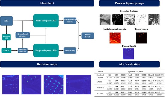
The remainder of this paper is organized as follows. The detailed introduction of our method is given in Section 2. Section 3 gives the experimental results and discussions including parameter analysis. Finally, we conclude this paper in Section 4.

2. Proposed Method

2.1. Low Rank Decomposition Model for Anomaly Detection

Assume an HSI dataset can be denoted as $\mathbf{X}\in {\mathbf{R}}^{h\times l\times B}$, where h and l are spatial size of the data, and B denotes the number of spectral bands. In order to facilitate subsequent processing, the 3-D data matrix is transformed into a 2-D matrix $\mathbf{X}={\left\{{\widehat{\mathbf{x}}}_i\right\}}_{i=1}^B\in {\mathbf{R}}^{N\times B}$, where $N=h\times l$ is the number of pixels in one spectral band. It is considered that background pixels from the same category are similar. For different categories, there is a strong correlation among pixels, but the difference between anomalous pixel and background pixel is much larger. Accordingly, the original dataset can be decomposed into two parts: background part and anomaly part, which can be written as

$$\mathbf{X}=\mathbf{DA}+\mathbf{E}$$

(1)

The first part of the equation representing the background describes that one background pixel can be approximated as a linear combination of several other background pixels. $\mathbf{D}\in {\mathbf{R}}^{N\times P}$ is the background dictionary, in which P is the number of atoms. $\mathbf{A}={\left\{{\widehat{\mathbf{a}}}_i\right\}}_{i=1}^B\in {\mathbf{R}}^{P\times B}$ is the coefficient matrix. E is the residual matrix containing the anomalies, which has the sparse property. The description above shows that the dataset can be well reconstructed through a good background dictionary.

To solve the problem (1), the ${\mathit{l}}_{21}$ norm is utilized to constrain the matrix E. The objective function of (1) is written as

$$\underset{\mathbf{A},\mathbf{E}}{min}{∥\mathbf{A}∥}_{*}+\lambda {∥\mathbf{E}∥}_{2,1}s.t.\mathbf{X}=\mathbf{DA}+\mathbf{E}$$

(2)

where ${∥·∥}_{*}$ is the nuclear norm. $\lambda$ > 0 is the tradeoff parameter to balance the low rank and sparsity. In [34,35], the low rankness principle has been proved to be superior at capturing the global characteristics of HSI data. However, some detailed characteristics of materials are usually hidden in the local structure. To represent the observed data more accurately, the local structure of the data should also be discovered. In target detection problems, many basic sparse-based detectors used both background and target pixels as training samples. For anomaly detection problem, as most of pixels belongs to background, they have a sparse representation in terms of the background dictionary. Therefore, by applying a sparse regularization to the coefficient matrix A, the local structure can be well described. In [15], the new objective function is written as:

$$\underset{\mathbf{A},\mathbf{E}}{min}{∥\mathbf{A}∥}_{*}+\beta {∥\mathbf{A}∥}_1+\lambda {∥\mathbf{E}∥}_{2,1}s.t.\mathbf{X}=\mathbf{DA}+\mathbf{E}$$

(3)

where $\beta$ > 0 is another parameter to trade off the low rankness and sparsity. E and A in (3) can be solved by the linearized alternating direction method with adaptive penalty (LADMAP) [14]. Usually, for the original HSI dataset, it is considered that the data lie in multiple subspaces, so from (2), the ${\mathit{l}}_{21}$ norm can be utilized to constrain most of elements of E to be zero. However, for some feature-based inputs, such as abundance vectors, it is usually considered that the input data lie in a single subspace, which means the anomalies from the same image may have different characteristics [18]. It is acceptable that the constraint of E should be appropriately relaxed so that there can be more nonzero elements in the matrix. Therefore, the ${\mathit{l}}_1$ norm is utilized to encourage E to be sparse, which can allow some nonzero values to exist in columns of the matrix. It is also reasonable to consider texture features lying in the single subspace when it serves as the input of LRD, and the ${\mathit{l}}_1$ norm is applied to constrain the model, which will be specifically described in the next subsection. Compared to multi subspace LRD, the objective function of the single subspace LRD model can be written as

$$\underset{\mathbf{A},\mathbf{E}}{min}{∥\mathbf{A}∥}_{*}+\lambda {∥\mathbf{E}∥}_{1}s.t.\mathbf{X}=\mathbf{DA}+\mathbf{E}$$

(4)

The optimization process of (4) is also different from that in (3). E and A can be solved by soft threshold method in [34]. The anomaly matrix E can be obtained after decomposing the matrix X. In order to generate the detection image, we sum along each column of E and reformat into the same spatial dimension of a single image in HSI.

2.2. Dictionary Construction Based on Graph Laplacian Matrix

As we have discussed above, dictionary construction plays a very important role in the LRD model. The clustering-based method is known as one kind of widely used strategy. However, the clustering performance strongly depends on the number of clusters K. If K is too small, some different materials may be clustered into one category. If k is too large, the same components will be divided into different categories, increasing the complexity of the image. In addition, as an unsupervised problem, making the assumption of known clustering number K is often unrealistic, especially for some HSI data with complex background structures. In our paper, inspired by [25], a graph Laplacian matrix-based method (GLM) is proposed for dictionary construction. It has big advantages of maintaining the principal structure and capturing the local information. On the other hand, it is also an adaptive method without significant parameter setting as K.

Assuming a weighted graphical set is represented as $\mathbf{G}=\left[\mathbf{V},\mathsf{\Gamma }\right]$, where V denotes a vertex set of order n, and $\mathsf{\Gamma }$ is an edge set specified by (a, b$w_{a,b}$). $a,b\in \mathbf{V}$, and $w_{a,b}$ is the edge weight from the vertex a to b. A graph signal that assigns a value to each vertex is denoted as $\mathbf{s}={\left[s_1,s_2...s_n\right]}^T$. Consequently, a weight matrix W can be obtained where $\mathbf{W}(a,b)=w_{a,b}$. According to [25], a combinatorial graph Laplacian matrix L is supposed to be captured first in order to compute the optimal decorrelating transform leveraging on spectral graph theory. Specifically, the graph Laplacian matrix L = D – W. D is called the degree matrix that is also a diagonal matrix and computed as follows:

$$D\left(a,b\right)=\left\{\begin{array}{c}\sum _{j=1}^n{w}_{a,j}ifa=b\\ 0,otherwise\end{array}\right.$$

(5)

Consequently, the weights of the matrix L are normalized to generate the symmetric normalized Laplacian matrix ${\mathbf{L}}^{sym}$, which is defined as (6). In practical processing, ${\mathbf{L}}^{sym}$ is more useful because it has some important properties. For instance, its eigenvalues are real and nonnegative. In this way, the spectrum of a symmetric normalized Laplacian has a good relationship with other graph invariance of general graphs, which cannot be achieved by other definitions [36].

$${\mathbf{L}}^{sym}={\mathbf{D}}^{-1/2}\mathbf{L}{\mathbf{D}}^{-1/2}$$

(6)

${\mathbf{L}}^{sym}$ has an eigen-decomposition as:

$${\mathbf{L}}^{sym}=\mathbf{U}\mathsf{\Lambda }{\mathbf{U}}^{-1}$$

(7)

where $\mathsf{\Lambda }$ is the diagonal matrix, whose diagonal elements are eigenvalues. U is the matrix composed of corresponding eigenvectors. As one of the most popular methods in signal processing, the Fourier transform can also be generalized to graphs, obtaining the so-called graph Fourier transform (GFT) [37]. Thus, here the matrix U is used to calculate the GFT of s, which is written as

$$\tilde{\mathbf{s}}={\mathbf{U}}^T\mathbf{s}$$

(8)

Accordingly, the inverse of GFT can be denoted as

$$\mathbf{s}=\mathbf{U}\tilde{\mathbf{s}}$$

(9)

For an HSI dataset, we define the data pixel x as equivalent to the graph signal s. Similar to RX, a graph Laplacian matrix based distance metric can be designed for computing the distance of x with its spectral and spatial neighbors. The metric can also be simplified to an eigenvalue-based expression through GFT, which is written as

$$\begin{array}{cc}\hfill \delta \left(x\right)& ={\mathbf{s}}^T\mathbf{L}\mathbf{s}\hfill \\ \hfill & ={\left(\mathbf{U}\tilde{\mathbf{s}}\right)}^T\mathbf{L}\left(\mathbf{U}\tilde{\mathbf{s}}\right)\hfill \\ \hfill & ={\tilde{\mathbf{s}}}^T\left({\mathbf{U}}^T\mathbf{L}\mathbf{U}\right)\tilde{\mathbf{s}}\hfill \\ \hfill & ={\tilde{\mathbf{s}}}^T\mathsf{\Lambda }\tilde{\mathbf{s}}\hfill \\ \hfill & =\sum _{j=1}^B{\lambda }_j{\tilde{s}}_j^2\hfill \end{array}$$

(10)

where ${\tilde{s}}_j$ is the jth element of $\tilde{\mathbf{s}}$. ${\lambda }_j$ ($1\le j\le B$) are eigenvalues in $\mathsf{\Lambda }$. In similar distance metric detectors, like RXD or Mahalanobis distance-based detectors, it can be observed that targets with small energy usually correspond to small eigenvalues, but their contribution to the detector is greater. This consideration is reasonable because if there is a small anomalous target in the image, it will not be visible in the principal component, but will appear in the smaller component [38]. From this perspective, when computing GFT in (10), the eigenvalues in $\mathsf{\Lambda }$ are sorted for increasing magnitude, i.e., ${\lambda }_1\le {\lambda }_2\le ...\le {\lambda }_B$. The eigenvectors in U are sorted accordingly. After setting a reasonable threshold, reliable background pixels can be obtained through GLM. Subsequently, in order to further extract robust elements from these plausible background pixels as the atoms of background dictionary, and reduce the computational burden, PCA is utilized to concentrate the energy into the first few principle components (PCs), and remove the redundant information, which will well underpin the subsequent processing.

2.3. Weight Selection of the Graph Model

In the graph model, the vertex set V contains B spectral nodes. Each pair of nodes is connected by an edge and a fully connected model can be generated. A simple model example of a three-band graph is shown in Figure 2a. Each edge has an assigned weight. In addition, due to the flexibility of the graph model, the topology can also be expanded spatially. The connectivity between adjacent nodes in both spatial and spectral domains can be established, as shown in Figure 2b.

Regarding to the weight determination, partial correlation [39] might be used as the weight under the assumption that the image follows a Gaussian Markov random field (GMRF) model. However, this approach still needs to compute the estimate and inversion of the covariance matrix, which has an expensive compute cost. In addition, the assumption of GMRF model, as the priori condition, is not followed by most of the practical images. The result will probably be unreliable if the assumption is not followed. Therefore, here we use the Cauchy function [40] as the weight function. It has no special requirements on the assumption of the probability distribution of the image, and has a fast calculation speed and good robustness. It has been commonly-used as a graph weight in other applications such as image segmentation and compression [41,42]. Assuming the band mean vector is represented as $\overline{\mu }={\left[{\mu }_1,{\mu }_2...{\mu }_b\right]}^T$, the weight of the edge connecting the band node a and b is set as

$$w_{ab}=\frac{1}{1+{\left(\frac{{\mu }_a-{\mu }_b}{\epsilon }\right)}^2}$$

(11)

where $\epsilon$ is the parameter that is used to normalize the band mean vectors. $\epsilon$ is set as $\epsilon =\frac{1}{B}{\sum }_{i=1}^B{\mu }_i$. In this way, the weight of the edge for each pair of spectral nodes is determined. When considering the case of 4-connected nodes, the graph model will be expanded to 5B nodes, as shown in Figure 2b. The weight matrix W will also have the size of 5B× 5B, the same size of Laplacian matrix L. We can construct the weight matrix as follows:

$${\mathbf{W}}_{(a,b)}=\left\{\begin{array}{cc}{w}_{ab}^{\prime },& aandbaredifferentspectralbands\\ w_{ab}^{\prime \prime },& aandbareadjcentnodesinoneband\\ 0,& otherwise\end{array}\right.$$

(12)

where spectral weights $w_{ab}^{\prime }$ can be estimated by (11). For spatial weights $w_{ab}^{\prime \prime }$, we set $w_{ab}^{\prime \prime }=1$, which is also the result calculated by (11).

2.4. Texture Features Extraction for Single Subspace LRD

Hyperspectral images contain not only rich spectral and spatial information, but also abundant information of textures. As an intrinsic feature of the image, the texture features of different categories in an HSI are also different. Therefore, through texture analysis, it can help distinguish different categories, thereby improving the accuracy [43,44]. There are many approaches for extracting texture features, including methods based on statistical characteristics, spatial frequency, and structure models [45]. In the statistics-based texture methods, texture is regarded as an expression of the correlation between adjacent pixels or adjacent regions. The gray level co-occurrence matrix (GLCM) expresses the textures by calculating the joint conditional probability density between the gray levels of each pixel, reflecting the correlation of the gray levels between any two points in the image and the statistical properties of the texture features [46,47]. GLCM is one of the most widely used methods for expressing texture features, and there have been a variety of different applications based on GLCM [48,49,50]. It describes the probability of two pixels with distance d and direction $\theta$ ($0^{\circ }$, ${45}^{\circ }$, ${90}^{\circ }$, ${135}^{\circ }$). Many GLCMs can be obtained according to values of (d, $\theta$) to analyze the spatial distribution pattern of image gray levels. GLCM is a symmetric matrix. If the roughness of a unit area $\Delta I$ with respect to the texture is very small, the element values in the matrix will be concentrated near the diagonal. Conversely, the element values will diffuse away from the diagonal. Haralick et al. [51] extracted fourteen characteristics from the GLCM. Here, the four most commonly-used ones are applied in our paper, which are second moment, contrast, entropy, and correlation. These textures are enough to describe the major features of an image. Assuming a GLCM with L gray value levels is denoted as P, the formula of each feature is demonstrated as

(i)

Second moment:

$$f_1=\sum _{i=0}^{L-1}\sum _{j=0}^{L-1}{\mathbf{P}}_{ij}^2$$

(13)

(ii)

Contrast:

$$f_2=\sum _{n=0}^{L-1}{n}^2\left\{\sum _{i=0}^{L-1}\sum _{j=0}^{L-1}{\mathbf{P}}_{ij}\right\}$$

(14)

(iii)

Entropy:

$$f_3=-\sum _{i=0}^{L-1}\sum _{j=0}^{L-1}{\mathbf{P}}_{ij}lo{g}_2{\mathbf{P}}_{ij}$$

(15)

(iv)

Correlation:

$$f_4=\sum _{i=0}^{L-1}\sum _{j=0}^{L-1}\frac{\left(ij\right){\mathbf{P}}_{ij}-u_i{u}_j}{s_i{s}_j}$$

(16)

where $u_i={\sum }_{i=0}^{L-1}{\sum }_{j=0}^{L-1}i·{\mathbf{P}}_{ij}$, $u_j={\sum }_{i=0}^{L-1}{\sum }_{j=0}^{L-1}j·{\mathbf{P}}_{ij}$, $s_i=\sqrt{{\sum }_{i=0}^{L-1}{\sum }_{j=0}^{L-1}{\mathbf{P}}_{ij}{(i-u_i)}^2}$, and $s_j=\sqrt{{\sum }_{i=0}^{L-1}{\sum }_{j=0}^{L-1}{\mathbf{P}}_{ij}{(j-u_j)}^2}$. We calculate the corresponding GLCM from four different directions $\theta$, and then obtain the average of each texture attribute. Thus, the four texture attributes of the mth band image can be represented as $f_m=\left[f_1,f_2,f_3,f_4\right]$. However, since there are numerous bands in an HSI, it is difficult to perform texture feature extraction for all bands, which is extremely laborious and has large calculation burden. Some traditional methods utilize PCA to generate a few PCs first, and then extract texture features on these components. It is worth noting that taking these principal components can retain over 90% of the energy, but we cannot guarantee that the remaining energy does not contain some or even more information of anomalies. If more components were selected, they would increase redundant information and computational burden. In this section, a de-noised version of GFT, as an extension of GFT, is described. As already discussed on GFT in (10), the de-noised version is expressed as

$${\delta }^p\left(\mathbf{x}\right)=\sum _{j=1}^p{\lambda }_j{\tilde{s}}_j^2$$

(17)

where the eigenvalues of $\mathsf{\Lambda }$ are sorted in increasing magnitude. $p\ll B$ and the orders of eigenvalues beyond p are considered to represent noisy and high frequency components, which will be discarded. The parameter p is determined according to the percentage of retained cumulative energy. Assuming the HSI dataset is denoted as $\mathbf{X}=\mathbf{I}=\left[{\mathbf{x}}_1,{\mathbf{x}}_2...{\mathbf{x}}_N\right]$, it can be expressed in terms of the Karhunen-Loève Transform (KLT) $\mathbf{Y}={\mathbf{V}}^T\mathbf{I}=\left[{\mathbf{y}}_1,{\mathbf{y}}_2...{\mathbf{y}}_N\right]$ as $e(\mathbf{I},p)={\sum }_{i=1}^N{\sum }_{j=1}^p{y}_{ij}^2$. Then, p is selected by $e(\mathbf{I},p)/e(\mathbf{I},\mathbf{B})\le \Psi$. In order to avoid the risk of losing anomalies as much as possible, here we set $\Psi$ = 0.99. Let $f_0=\delta \left(\mathbf{X}\right)$, and we combine it with the texture features. The resulting extended feature map can be represented as $\mathbf{F}=\left[f_0,f_1,f_2,f_3,f_4\right]$. The dimensionality of the matrix F is five. Each feature map is shown in Figure 3.

For the feature map F, the four texture features $\left[f_1,f_2,f_3,f_4\right]$ are from one GLCM, which is generated from the de-noised version of GFT $f_0$. There are high correlations among texture features. Therefore, it is reasonable to consider that the feature vectors lie in a single subspace, as we discussed in the previous subsection. Accordingly, the constraint of the residual matrix E in LRD model should be appropriately relaxed so that there can be more nonzero elements in the matrix. We use $l_1$ norm instead of $l_{21}$ norm to encourage matrix E to be sparse. Therefore, the objective function of the single subspace LRD model is written as (4). It can be solved by the soft threshold method in [34].

For the original HSI dataset, the sparse matrix obtained by multi-subspace LRD, denoted as ${\mathbf{E}}_0$, and the sparse matrix for texture features obtained by single-subspace LRD, denoted as ${\mathbf{E}}_1$, can be incorporated to detect the anomalies while improving the detection accuracy. The amount of information in the original image data is greater than feature vectors, and the basis in the dictionary constructed from datasets can represent the image pixels more completely. In comparison, what we should admit is that for the extended feature maps (one de-noised GFT map and four texture features calculated by GLCM) as the input to the single-subspace LRD, the amount of information cannot be compared with the original data. Moreover, the graph dictionary is also constructed by the feature vectors. All these factors make some of the anomalous elements in the resulting sparse part not represented. However, the main purpose of using texture features is to strengthen the real anomalies while further suppressing the background, which is equivalent to helping the original sparse part ${\mathbf{E}}_0$ to enhance the discrimination. The sparse matrix by texture features ${\mathbf{E}}_1$ have good ability to accomplish this objective. As one of the most widely used methods, the weighted average-based method is favored here because it can integrate the two results simply and steady. It performs linear average weighting on the gray values of the two images to generate a new image. For different image data, we can find the optimal fusion result by adjusting the value of weight. The procedure of the proposed GLRD_TFE is summarized in Algorithm 1.

Algorithm 1. Anomaly detection via graph dictionary-based LRD with texture feature extraction

1: Input: hyperspectral image X; parameters: $\lambda$, $\beta$, ${\lambda }_1$, $(w_t,w_t)$, and $({\omega }_0,{\omega }_1)$.

2.1: Obtain the weight matrix W by

${\mathbf{W}}_{(a,b)}=\left\{\begin{array}{cc}{w}_{ab}^{\prime },& aandbaredifferentspectralbands\\ w_{ab}^{\prime \prime },& aandbareadjcentnodesinoneband\\ 0,& otherwise\end{array}\right.$

where $w_{ab}=\frac{1}{1+{\left(\frac{{\mu }_a-{\mu }_b}{\epsilon }\right)}^2}$, $w_{ab}^{\prime \prime }=1$

2.2: L = D − W, D is calculated by (5). Then $\mathbf{L}=\mathbf{U}\mathsf{\Lambda }{\mathbf{U}}^{-1}$.

2.3: Construct the graph-based background dictionary D by Equation (10).

3: Solve the objective function of the multi-subspace LRD using LADMAP:

$\underset{\mathbf{A},\mathbf{E}}{min}{∥\mathbf{A}∥}_{*}+\beta {∥\mathbf{A}∥}_1+\lambda {∥\mathbf{E}∥}_{2,1}s.t.\mathbf{X}=\mathbf{DA}+\mathbf{E}$

Obtain the sparse matrix ${\mathbf{E}}_0$.

4: Calculate the de-noised version of GFT $f_0$. Generate the GLCM of $f_0$ with

four texture features $f_m=\left[f_1,f_2,f_3,f_4\right]$, and obtaining the extended feature $\mathbf{F}=\left[f_0,f_1,f_2,f_3,f_4\right]$.

5: Solve the objective function of the single subspace LRD using soft threshold method in [34]:

$\underset{\mathbf{A},\mathbf{E}}{min}{∥\mathbf{A}∥}_{*}+\lambda {∥\mathbf{E}∥}_{1}s.t.\mathbf{X}=\mathbf{DA}+\mathbf{E}$

Obtain the sparse matrix ${\mathbf{E}}_1$.

6: Fuse two sparse matrices by weighted average-based method:

$\mathbf{Re}={\omega }_0·{\mathbf{E}}_0+{\omega }_1·{\mathbf{E}}_1,s.t.{\omega }_0+{\omega }_1=1$

7: Output: Final detection result Re.

3. Experimental Results and Analysis

In this section, we compare the proposed GLRD_TFE algorithm with a series of classical or widely used anomaly detection algorithms, such as GRX [5], LRX [6], KLRX [7], LAD [25], CRD [11], BJSRD [12], and LRASR [15]. All the experiments are conducted on a PC with Intel Core i5-9300H 2.40 GHz and 16 GB RAM.

In order to clearly observe the detection results, we show the color detection maps of all algorithms by experiment. Different colors indicate different response intensities to the components, the brighter the color, the stronger the response. In addition, the receiver operating characteristic (ROC) curves with pointwise confidence intervals [52] are utilized to further investigate the detection performance quantitatively. Furthermore, the area under ROC curve (AUC) is also computed to evaluate the performance of these methods.

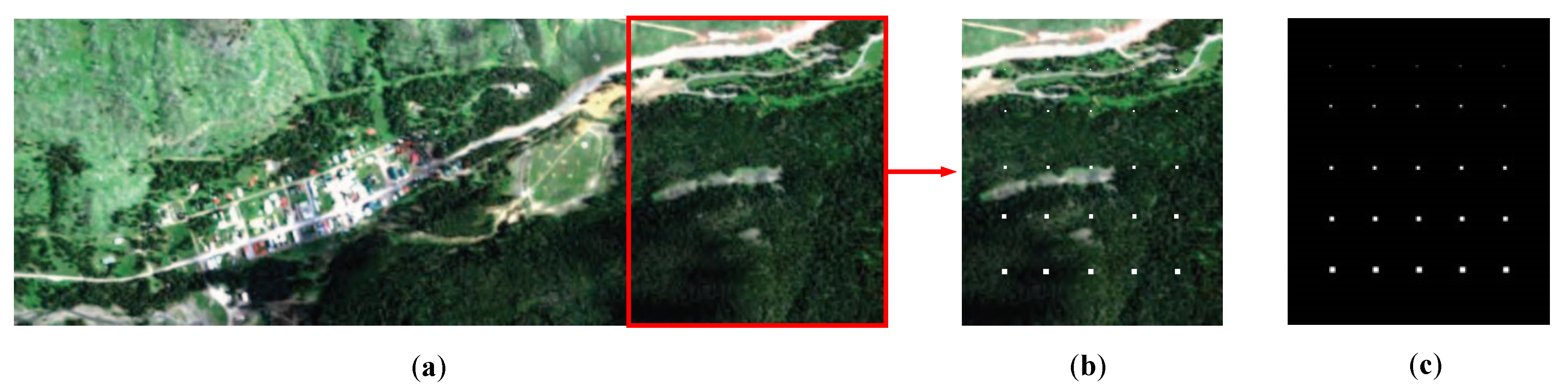
3.1. HSI Dataset Descriptions

In the experiment, we use both simulated and real HSI datasets to evaluate the proposed method. The first one is a simulated data generated based on the HyMap dataset downloaded from the Rochester Institute of Technique (RIT) (http://dirsapps.cis.rit.edu/blindtest/information/) [53]. It was collected in a small town of Cook City, MT, USA. The whole dataset has a size of 280 × 800 pixels with 126 spectral bands, as shown in Figure 4a. After removing the bad bands that correspond to low SNR, water absorption, and poor response, there are 119 bands left. A sub-region with a size of 280 × 240 pixels is selected to form the simulated data. The background contains a road and different kinds of vegetation. The simulated targets are generated according to [54]. A desired target t is embedded into the background b through the abundance fraction f to obtain a synthetic sub-pixel target z, which follows the formula:

$$\mathbf{z}=f·\mathbf{t}+(1-f)·\mathbf{b}$$

(18)

There are 25 anomaly targets (1 × 1, 2 × 2, 3 × 3, 4 × 4, and 5 × 5) implanted in the first dataset, distributed in five rows and five columns. The value of f is 0.05, 0.1, 0.2, 0.3, and 0.4 corresponding to each column, respectively. The spectrum of anomaly target t is selected outside the sub-region. The false color image and the ground-truth map are shown in Figure 4b,c, respectively.

The second dataset was collected by the Airborne Visible/Infrared Imaging Spectrometer (AVIRIS), which is over San Diego, CA, USA. There are 224 spectral bands. We call it AVIRIS–I in this paper. After eliminating the low SNR and bad bands (1–6, 33–35, 97, 107–113, 153–166, and 221–224), 189 available bands are retained. The whole size of the dataset is 400 × 400 pixels. An upper left sub-region containing anomalous targets is selected for the experiment, whose size is 100 × 100 pixels. The targets of the scene refer to three airplanes with 57 pixels totally. The original dataset, the false color image, and the ground-truth map are shown in Figure 5a–c, respectively.

The third dataset is also acquired by AVIRIS, which is called AVIRIS–II. The sub-region is selected from the lower left corner of San Diego image. There are 22 small aircrafts in the scene considered as anomalous targets. The size of scene is 60 × 60 pixels which contains 214 anomalous pixels, as shown in Figure 6b,c.

The fourth dataset is an Hyperspectral Digital Imagery Collection Experiment (HYDICE) HSI dataset from an aircraft platform. The scene covers an urban area, which is composed of a vegetation area, a construction area, and several roads, including some vehicles. The whole dataset has a size of 307 × 307 pixels with 210 spectral bands, shown in Figure 7a. After removing the bands of the water absorption regions and low signal-to-noise ratio (1–4, 76, 87, 101–111, 136–153, and 198–210), 162 bands are retained. In the experiment, we capture a region from the upper-right of the whole scene and obtain a sub-region with a size of 80 × 100. There are 21 pixels of vehicles as anomalous targets, as shown in Figure 7b,c.

3.2. Detection Performance

We compare the proposed GLRD_TFE algorithm with seven state-of-the-art detectors to evaluate the detection performance: GRX, LRX, KLRX, LAD, CRD, BJSRD and LRASR. The sizes of dual-windows in LRX and KLRX ($w_{in}$, $w_{out}$) are set as (7, 13) for two AVIRIS datasets, and (5, 7) for the simulated and HYDICE data. For CRD, the sizes of dual-windows are set to be the same as LRX. LAD has no specific parameters that significantly affect the performances. In BJSRD, the important parameters include the sizes of three windows: inner window, outer window, and search window, which are denoted as ($w_{in}$, $w_{out}$, $w_{se}$). For the simulated and HYDICE data, ($w_{in}$, $w_{out}$, $w_{se}$) = (9, 11, 13). For the two AVIRIS datasets, ($w_{in}$, $w_{out}$, $w_{se}$) is set to (13, 15, 17). In addition, the other parameter, the upper bound of joint sparsity, is set to 6 for all four HSIs. In LRASR, there are three important parameters, the number of clusters K and two tradeoff parameters $\lambda$ and $\beta$ in LRD model. K is set as 6 for the simulated dataset and two AVIRIS datasets. K = 7 for HYDICE dataset. [$\lambda$, $\beta$] ∈ [0.1, 0.01] in two AVIRIS datasets. For the simulated dataset, the two parameters are more stable, and [$\lambda$, $\beta$] ∈ [0.01, 0.01] for HYDICE dataset. Regarding to the proposed GLRD_TFE method, the important parameters are: tradeoff parameters $\lambda$ and $\beta$ in the multi-subspace LRD, another tradeoff parameter ${\lambda }_1$ in the single subspace LRD, the size of the windows ($w_t$, $w_t$) selected on the GLCM when calculating texture features, and the weight values of the fusion for two matrices (${\omega }_0$, ${\omega }_1$). The detailed analysis will be discussed in the following Section 4.

The detection maps of all compared algorithms for the four HSI datasets are respectively shown in Figure 8, Figure 9, Figure 10 and Figure 11. It can be seen that GRX and LRX can hardly detect the targets clearly in the first three datasets. In the result of KLRX, there are still many targets not detected, even if the detection results become clearer. In addition, there is also some loss in the edge area of the LRX and KLRX results due to the sliding of the dual-windows. In the last HYDICE dataset, part of anomalous targets can be detected by GRX and LRX. However, GRX does not suppress the background very well, while LRX suppresses too much, and even includes part of anomalous pixels. LAD has a good detection performance in AVIRIS–II dataset, which gives us a deep impression. The edges of the target aircraft can be clearly detected, but it has poor performances in other datasets. Specifically, for the simulated data, a large number of background components are falsely detected, and almost all real anomalies are suppressed, which is the same situation for HYDICE dataset. For AVIRIS–II dataset, several anomalous targets are not successfully detected, and the background component with high contrast in the upper right corner of the image greatly increases the false alarm. CRD can detect most anomalous targets in the AVIRIS–II and HYDICE dataset, while some target pixels in the simulated dataset and AVIRIS–I dataset are suppressed together as well with the background components. In AVIRIS–II dataset, the background in the upper right corner of the scene is not suppressed effectively. BJSRD can smoothly suppress the background of different datasets. Anomalous targets are also affected at the same time. Some relatively weak targets are suppressed along with the background. LRASR can detect the anomalies correctly in all four datasets, but similar to CRD and BJSRD, its response to darker target pixels is weak. Furthermore, LRASR cannot effectively suppress background areas with strong energy in both AVIRIS–I and AVIRIS–II datasets. For the proposed GLRD_TFE, it can be seen that not only bright targets, but also dark target pixels can be successfully detected. On the other hand, the texture feature-based processing in GLRD_TFE successfully suppresses high-intensity background components similar to the targets, and greatly improves the detection performance.

To have a quantitative assessment for the performance of all compared algorithms in different datasets, we draw the ROC curves with pointwise confidence intervals [52] and show them in Figure 12. In the simulated dataset, the curves of both LRASR and GLRD_TFE show very good performances. LRASR suppresses the background well but also suppresses weaker targets, while GLRD_TFE can clearly show all targets, so its curve is also higher. The LRASR method shows a stable and robust performance in the simulated and AVIRIS–I datasets. However, in the last two datasets, it is affected to a certain extent. The reason is that for AVIRIS–II dataset, the complex background in the upper right corner is not suppressed, and for HYDICE dataset, some targets are over-suppressed due to their small sizes. In addition, CRD also shows a good performance while it suffers from the sensitivity to the window size, especially for HYDICE dataset, which has a cluttered background. LAD reveals exceptional detection ability in AVIRIS–I dataset. The reason is that the difference between the spectrum of background and anomalies is large, which can be better separated in the eigenvalue decomposition of the graph Laplacian matrix. For other datasets, LAD does not show surprises like this. In general, our proposed GLRD_TFE has the best performance for each dataset. As shown in detection maps, it is obvious to see that those backgrounds with strong interference are almost removed, and targets of different sizes are retained. Furthermore, the area under the curve (AUC) values of each algorithm are summarized in

Table 1. AUC values of detection results by all comparison methods in four datasets.

Dataset	Algorithm/AUC Value
Simulated dataset	RX	LRX	KLRX	LAD	CRD	BJSRD	LRASR	GLRD_TFE
	0.7771	0.7565	0.9690	0.5408	0.7565	0.9572	0.9625	0.9845
AVIRIS–I	RX	LRX	KLRX	LAD	CRD	BJSRD	LRASR	GLRD_TFE
	0.9217	0.7073	0.9825	0.9975	0.9814	0.9928	0.9853	0.9962
AVIRIS–II	RX	LRX	KLRX	LAD	CRD	BJSRD	LRASR	GLRD_TFE
	0.7638	0.6319	0.7880	0.8920	0.9224	0.9014	0.8275	0.9699
HYDICE	RX	LRX	KLRX	SSRX	CRD	BJSRD	LRASR	GLRD_TFE
	0.8508	0.7702	0.7450	0.9155	0.9110	0.9198	0.9110	0.9900

. We can see from Table 1 that the proposed GLRD_TFE has the highest values in three different datasets, and it has the same great performance as LAD in the other dataset. Overall, it demonstrates that the performance of GLRD_TFE outperforms others.

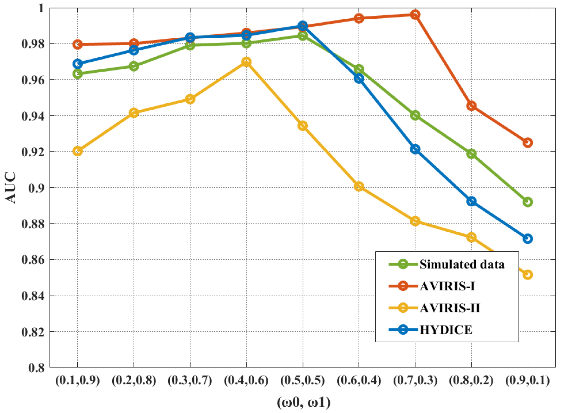
4. Parameter Discussion

The low rank decomposition model is utilized to obtain the initial anomaly matrix. It involves two tradeoff parameters $\beta$ and $\lambda$ in the multi-subspace LRD. Both of the parameters determine the degree of separation between the sparse matrix E and the background component DZ. Both $\beta$ and $\lambda$ are chosen from {0.001, 0.01, 0.05, 0.1, 0.2, 0.3, 0.4, 0.5}. The change is shown in Figure 13. It reveals that the performance of GLRD_TFE is stable with the change of $\beta$, but more sensitive to $\lambda$. Therefore, we choose $\beta$ = 0.1 for all datasets. What four datasets have shown in common is that when $\lambda$ < 0.01, the performance of the algorithm is poor. Furthermore, the performance is relatively stable for the simulated data. For AVIRIS–I and AVIRIS–II datasets, as $\lambda$ increases, both of the AUC values decrease due to their similar background uniformity and target sizes. For the HYDICE dataset, when $\lambda$ > 0.1 and $\beta$ > 0.1, the AUC value has a slight decrease. Therefore, we choose $\lambda$ = 0.01 for the first three datasets and $\lambda$ = 0.05 for the HYDICE dataset.

For texture-based processing, there are two important parameters: the tradeoff parameter ${\lambda }_1$ in single subspace LRD and the size of the windows ($w_t$, $w_t$) selected on the GLCM. The change of AUC value with ${\lambda }_1$ and ($w_t$, $w_t$) is shown in Figure 14. We can see that the detection performance for texture features in LRD is very sensitive to ($w_t$, $w_t$). Specifically, for the simulated, AVIRIS–II, and HYDICE datasets, the best result can be obtained when the ($w_t$, $w_t$) is (3, 3). The best window parameter for AVIRIS–I is (5, 5). As for the parameter ${\lambda }_1$, the sensitivity range of ${\lambda }_1$ is different for different datasets. The range in the first dataset is 0.001, 0.005, 0.01, 0.05, 0.1, 0.5, and the value of ${\lambda }_1$ is set to 0.005 for best performance. For the second dataset, the range of value of ${\lambda }_1$ is {0.01, 0.05, 0.1, 0.2, 0.5, 0.7}, and ${\lambda }_1$ = 0.05 achieves the best. For the last two datasets, the ranges of ${\lambda }_1$ are respectively {0.001, 0.005, 0.01, 0.03, 0.05, 0.09} and {0.1, 0.12, 0.14, 0.16, 0.2, 0.3}. For optimal performance, ${\lambda }_1$ is set to 0.01 and 0.12, respectively.

In addition, the weight values of the fusion for two matrices (${\omega }_0$, ${\omega }_1$) will also affect the final detection performance to a certain extent. ${\omega }_0$ refers to the weight of residual matrix obtained by the multiple subspace LRD model, and ${\omega }_1$ refers to the weight of the result of texture from the single subspace LRD model. The change curves of the detection performances with the values of fusion weight are shown in Figure 15. It can be seen that the optimal fusion result for the simulated dataset is obtained when (${\omega }_0$, ${\omega }_1$) is set to (0.7, 0.3). Since both the background and targets are too suppressed in the result of texture, more weight should be assigned to the result of the original dataset, and meanwhile the contribution of the texture feature is reduced. Thus, all anomalous target pixels can be displayed while the redundant background can be controlled. For AVIRIS–I and AVIRIS–II datasets, (${\omega }_0$, ${\omega }_1$) is set to (0.5, 0.5) in optimal. The parameters for HYDICE dataset are set to (0.4, 0.6) because more background components contained in the result of HSI need to be suppressed with the help of texture vectors. On the other hand, it is also observed that when the result of the original data occupies a large proportion, the change of AUC is smaller than that of texture features. This shows that the robustness of the result of texture feature is weaker than that of the original image. The detection performance itself is also weaker than that of the original data. In addition, it suppresses the background and also greatly affects some target pixels.

5. Conclusions

In this paper, we propose a novel hyperspectral anomaly detection algorithm called GLRD_TFE. Based on the graph Laplacian matrix and graph Fourier transform, a new background dictionary is constructed without considering prior parameters or solving the high-dimensional covariance matrix. It also maintains the connectivity between elements. The HSI can be decomposed into the reconstruction background part and the initial anomaly part by utilizing the multiple subspace LRD. On the other hand, the gray level co-occurrence matrix is calculated based on a de-noised version of GFT that concentrates most of the energy in the data. Four major texture features are extracted from the GLCM, and regarded as the input data of the single subspace LRD. The proposed algorithm proves the effectiveness of texture features to suppress background and improve the detection accuracy. The targets are distinguished both spatially and spectrally through graph theory, low rank model, and texture features. The experiments on synthetic and real datasets showed that GLRD_TFE achieved high detection performances. The quantitative evaluations, i.e., ROC and AUC, prove that the proposed method offers higher performance than other seven comparison methods.

References

1. Stein, D.W.; Beaven, S.G.; Hoff, L.E.; Winter, E.M.; Schaum, A.P.; Stocker, A.D. Anomaly detection from hyperspectral imagery. IEEE Signal Proc. Mag. 2002, 19, 58–69. [Google Scholar] [CrossRef] [Green Version]
2. Goetz, A.F.; Vane, G.; Solomon, J.E.; Rock, B.N. Imaging Spectrometry for Earth Remote Sensing. Science 1985, 228, 1147–1153. [Google Scholar] [CrossRef] [PubMed]
3. Du, B.; Zhang, L. Random-selection-based anomaly detector for hyperspectral imagery. IEEE Trans. Geosci. Remote Sens. 2011, 49, 1578–1589. [Google Scholar] [CrossRef]
4. Khazai, S.; Safari, A.; Mojaradi, B.; Homayouni, S. An approach for subpixel anomaly detection in hyperspectral images. IEEE J. Sel. Top. Appl. Earth Obs. Remote Sens. 2013, 6, 769–778. [Google Scholar] [CrossRef]
5. Reed, I.S.; Yu, X. Adaptive multiple-band CFAR detection of an optical pattern with unknown spectral distribution. IEEE Trans. Acoust. Speech Signal Process. 1990, 38, 1760–1770. [Google Scholar] [CrossRef]
6. Chen, J.Y.; Reed, I.S. A detection algorithm for optical targets in clutter. IEEE Trans. Aerosp. Electron. Syst. 1987, 23, 46–59. [Google Scholar] [CrossRef]
7. Kwon, H.; Nasrabadi, N.M. Kernel RX-algorithm: A nonlinear anomaly detector for hyperspectral imagery. IEEE Trans. Geosci. Remote Sens. 2005, 43, 388–397. [Google Scholar] [CrossRef]
8. Wright, J.; Yang, A.Y.; Ganesh, A.; Sastry, S.S.; Ma, Y. Robust face recognition via sparse representation. IEEE Trans. Pattern Anal. Mach. Intell. 2009, 31, 210–227. [Google Scholar] [CrossRef] [Green Version]
9. Yang, J.; Wright, J.; Huang, T.; Ma, Y. Image super-resolution as sparse representation of raw image patches. In Proceedings of the IEEE Conference on Computer Vision and Pattern Recognition (CVPR), Anchorage, AK, USA, 23–28 June 2008; pp. 1–8. [Google Scholar]
10. Chen, Y.; Nasrabadi, N.M.; Tran, T.D. Sparse representation for target detection in hyperspectral imagery. IEEE J. Sel. Top. Signal Process. 2011, 5, 629–640. [Google Scholar] [CrossRef]
11. Li, W.; Du, Q. Collaborative representation for hyperspectral anomaly detection. IEEE Trans. Geosci. Remote Sens. 2014, 53, 1463–1474. [Google Scholar] [CrossRef]
12. Li, J.; Zhang, H.; Zhang, L.; Ma, L. Hyperspectral anomaly detection by the use of background joint sparse representation. IEEE J. Sel. Top. Appl. Earth Obs. Remote Sens. 2015, 8, 2523–2533. [Google Scholar] [CrossRef]
13. Sun, W.; Liu, C.; Li, J.; Lai, Y.M.; Li, W. Low-rank and sparse matrix decomposition-based anomaly detection for hyperspectral imagery. J. Appl. Remote. Sens. 2014, 8, 083641. [Google Scholar] [CrossRef]
14. Zhang, Y.; Du, B.; Zhang, L.; Wang, S. A low-rank and sparse matrix decomposition-based mahalanobis distance method for hyperspectral anomaly detection. IEEE Trans. Geosci. Remote Sens. 2015, 54, 1376–1389. [Google Scholar] [CrossRef]
15. Xu, Y.; Wu, Z.; Li, J.; Plaza, A.; Wei, Z. Anomaly detection in hyperspectral images based on low-rank and sparse representation. IEEE Trans. Geosci. Remote Sens. 2016, 54, 1990–2000. [Google Scholar] [CrossRef]
16. Liu, G.; Lin, Z.; Yan, S.; Sun, J.; Yu, Y.; Ma, Y. Robust recovery of subspace structures by low-rank representation. IEEE Trans. Pattern Anal. Mach. Intell. 2013, 35, 171–184. [Google Scholar] [CrossRef] [PubMed] [Green Version]
17. Song, S.; Zhou, H.; Gu, L.; Yang, Y.; Yang, Y. Hyperspectral Anomaly Detection via Tensor-Based Endmember Extraction and Low-Rank Decomposition. IEEE Geosci. Remote. Sens. Lett. 2019, 17, 1772–1776. [Google Scholar] [CrossRef]
18. Qu, Y.; Wang, W.; Guo, R.; Ayhan, B.; Kwan, C.; Vance, S.; Qi, H. Hyperspectral anomaly detection through spectral unmixing and dictionary-based low-rank decomposition. IEEE Trans. Geosci. Remote Sens. 2018, 56, 4391–4405. [Google Scholar] [CrossRef]
19. Li, F.; Zhang, X.; Zhang, L.; Jiang, D.; Zhang, Y. Exploiting structured sparsity for hyperspectral anomaly detection. IEEE Trans. Geosci. Remote Sens. 2018, 56, 4050–4064. [Google Scholar] [CrossRef]
20. Baterina, A.V.; Oppus, C. Image edge detection using ant colony optimization. WSEAS Trans. Signal Process. 2010, 6, 58–67. [Google Scholar]
21. Mao, Q.; Wang, L.; Tsang, I.W.; Sun, Y. Principal graph and structure learning based on reversed graph embedding. IEEE Trans. Pattern Anal. Mach. Intell. 2016, 395, 2227–2241. [Google Scholar] [CrossRef]
22. Barnes, J.A.; Harary, F. Graph theory in network analysis. Soc. Netw. 1983, 5, 235–244. [Google Scholar] [CrossRef] [Green Version]
23. Santner, J.; Pock, T.; Bischof, H. Interactive multi-label segmentation. In Asian Conference on Computer Vision, Proceedings of the ACCV 2010: Computer Vision, Queenstown, New Zealand, 8–12 November 2010; Springer: Berlin/Heidelberg, Germany, 2010; pp. 397–410. [Google Scholar]
24. Akoglu, L.; Tong, H.; Koutra, D. Graph based anomaly detection and description: A survey. Data Min. Knowl. Discov. 2015, 29, 626–688. [Google Scholar] [CrossRef] [Green Version]
25. Verdoja, F.; Grangetto, M. Graph Laplacian for image anomaly detection. Mach. Vis. Appl. 2020, 31, 11. [Google Scholar] [CrossRef] [Green Version]
26. Zhao, R.; Zhang, L. GSEAD: Graphical scoring estimation for hyperspectral anomaly detection. IEEE J. Sel. Top. Appl. Earth Obs. Remote Sens. 2016, 10, 725–739. [Google Scholar] [CrossRef]
27. Yuan, Y.; Ma, D.; Wang, Q. Hyperspectral anomaly detection by graph pixel selection. IEEE Trans. Cybern. 2015, 46, 3123–3134. [Google Scholar] [CrossRef] [PubMed]
28. Wang, X.; Georganas, N.D.; Petriu, E.M. Fabric texture analysis using computer vision techniques. IEEE Trans. Instrum. Meas. 2010, 60, 44–56. [Google Scholar] [CrossRef]
29. Malik, J.; Belongie, S.; Leung, T.; Shi, J. Contour and texture analysis for image segmentation. Int. J. Comput. Vis. 2001, 43, 7–27. [Google Scholar] [CrossRef]
30. Kiechle, M.; Storath, M.; Weinmann, A.; Kleinsteuber, M. Model-based learning of local image features for unsupervised texture segmentation. IEEE Trans. Image Process. 2018, 27, 1994–2007. [Google Scholar] [CrossRef] [Green Version]
31. Pla, F.; Gracia, G.; García-Sevilla, P.; Mirmehdi, M.; Xie, X. Multi-spectral texture characterisation for remote sensing image segmentation. In Iberian Conference on Pattern Recognition and Image Analysis, Proceedings of the IbPRIA 2009: Pattern Recognition and Image Analysis, Póvoa de Varzim, Portugal, 10–12 June 2009; Springer: Berlin/Heidelberg, Germany, 2009; pp. 257–264. [Google Scholar]
32. Liao, S.; Law, M.W.; Chung, A.C. Dominant local binary patterns for texture classification. IEEE Trans. Image Process. 2009, 18, 1107–1118. [Google Scholar] [CrossRef] [Green Version]
33. Li, J.; Xi, B.; Li, Y.; Du, Q.; Wang, K. Hyperspectral classification based on texture feature enhancement and deep belief networks. Remote Sens. 2018, 10, 396. [Google Scholar] [CrossRef] [Green Version]
34. Liu, G.; Lin, Z.; Yu, Y. Robust subspace segmentation by low-rank representation. In Proceedings of the 27th International Conference on Machine Learning (ICML-10), Haifa, Israel, 21–24 June 2010; pp. 663–670. [Google Scholar]
35. Liu, G.; Yan, S. Latent low-rank representation for subspace segmentation and feature extraction. In Proceedings of the International Conference on Computer Vision (ICCV), Barcelona, Spain, 6–13 November 2011; pp. 1615–1622. [Google Scholar]
36. Chung, F.R.; Graham, F.C. Spectral Graph Theory; American Mathematical Soc.: Providence, RI, USA, 1997; Volume 92, Available online: http://www.math.ucsd.edu/~fan/research/revised.html (accessed on 3 December 2020).
37. Sandryhaila, A.; Moura, J.M. Discrete signal processing on graphs: Graph fourier transform. In Proceedings of the IEEE International Conference on Acoustics, Speech and Signal Processing, Vancouver, BC, Canada, 26–31 May 2013; pp. 6167–6170. [Google Scholar]
38. Chang, C.I.; Chiang, S.S. Anomaly detection and classification for hyperspectral imagery. IEEE Trans. Geosci. Remote Sens. 2002, 40, 1314–1325. [Google Scholar] [CrossRef] [Green Version]
39. Zhang, C.; Florêncio, D. Analyzing the optimality of predictive transform coding using graph-based models. IEEE Signal Process Lett. 2012, 20, 106–109. [Google Scholar] [CrossRef]
40. Grady, L.J.; Polimeni, J.R. Applied Analysis on Graphs for Computational Science; Springer Science & Business Media: London, UK, 2010; Available online: https://0-www-springer-com.brum.beds.ac.uk/gp/book/9781849962896 (accessed on 3 December 2020).
41. Black, M.J.; Sapiro, G.; Marimont, D.H.; Heeger, D. Robust anisotropic diffusion. IEEE Trans. Image Process. 1998, 7, 421–432. [Google Scholar] [CrossRef] [PubMed] [Green Version]
42. Fracastoro, G.; Magli, E. Predictive graph construction for image compression. In Proceedings of the IEEE International Conference on Image Processing (ICIP), Quebec City, QC, Canada, 27–30 September 2015; pp. 2204–2208. [Google Scholar]
43. Qian, Y.; Ye, M.; Zhou, J. Hyperspectral image classification based on structured sparse logistic regression and three-dimensional wavelet texture features. IEEE Trans. Geosci. Remote Sens. 2012, 51, 2276–2291. [Google Scholar] [CrossRef] [Green Version]
44. Zhang, X.; Younan, N.H.; O’Hara, C.G. Wavelet domain statistical hyperspectral soil texture classification. IEEE Trans. Geosci. Remote Sens. 2005, 43, 615–618. [Google Scholar] [CrossRef]
45. Faugeras, O.D.; Pratt, W.K. Decorrelation methods of texture feature extraction. IEEE Trans. Pattern Anal. Mach. Intell. 1980, 4, 323–332. [Google Scholar] [CrossRef]
46. Soh, L.K.; Tsatsoulis, C. Texture analysis of SAR sea ice imagery using gray level co-occurrence matrices. IEEE Trans. Geosci. Remote Sens. 1999, 37, 780–795. [Google Scholar] [CrossRef] [Green Version]
47. Sebastian, V.B.; Unnikrishnan, A.; Balakrishnan, K. Gray level co-occurrence matrices: Generalisation and some new features. arXiv 2012, arXiv:1205.4831. [Google Scholar]
48. Partio, M.; Cramariuc, B.; Gabbouj, M.; Visa, A. Rock texture retrieval using gray level co-occurrence matrix. In Proceedings of the 5th Nordic Signal Processing Symposium, Bergen, Norway, 4–7 October 2002; Volume 75. [Google Scholar]
49. De Siqueira, F.R.; Schwartz, W.R.; Pedrini, H. Multi-scale gray level co-occurrence matrices for texture description. Neurocomputing 2013, 120, 336–345. [Google Scholar] [CrossRef]
50. Beura, S.; Majhi, B.; Dash, R. Mammogram classification using two dimensional discrete wavelet transform and gray-level co-occurrence matrix for detection of breast cancer. Neurocomputing 2015, 154, 1–14. [Google Scholar] [CrossRef]
51. Haralick, R.M.; Shanmugam, K.; Dinstein, I.H. Textural features for image classification. IEEE Trans. Syst. Man Cybern. 1973, 6, 610–621. [Google Scholar] [CrossRef] [Green Version]
52. Kerekes, J. Receiver operating characteristic curve confidence intervals and regions. IEEE Geosci. Remote Sens. Lett. 2008, 5, 251–255. [Google Scholar] [CrossRef] [Green Version]
53. Snyder, D.; Kerekes, J.; Fairweather, I.; Crabtree, R.; Shive, J.; Hager, S. Development of a web-based application to evaluate target finding algorithms. In Proceedings of the IGARSS 2008—2008 IEEE International Geoscience and Remote Sensing Symposium, Boston, MA, USA, 7–11 July 2008; Volume 2, pp. II-915–II-918. [Google Scholar]
54. Stefanou, M.S.; Kerekes, J.P. A method for assessing spectral image utility. IEEE Trans. Geosci. Remote Sens. 2009, 47, 1698–1706. [Google Scholar] [CrossRef]
Figure 1. Flowchart of the proposed graph dictionary-based low rank decomposition with texture feature extraction (GLRD_TFE) method.
Remotesensing 12 03966 g001
Figure 2. Example of connectivity on graph model. (a) Fully connected on three spectral bands. (b) Fully connected on four spatial nodes.
Remotesensing 12 03966 g002
Figure 3. Extended feature maps F = [ f 0 , f 1 , f 2 , f 3 , f 4 ]. (a) f 0 : result map through de-noised graph Fourier transform (GFT); (b) f 1 : second moment; (c) f 2 : contrast; (d) f 3 : entropy; (e) f 4 : correlation.
Remotesensing 12 03966 g003
Figure 4. Dataset of synthetic targets for experiment. (a) False color image of the whole scene; (b) false color image of the detection area; (c) ground-truth of simulated dataset.
Remotesensing 12 03966 g004
Figure 5. Descriptions of Airborne Visible/Infrared Imaging Spectrometer (AVIRIS)–I dataset. (a) False color image of the whole scene; (b) false color image of the detection area; (c) ground-truth of AVIRIS–I dataset.
Remotesensing 12 03966 g005
Figure 6. Descriptions of AVIRIS–II dataset. (a) False color image of the whole scene; (b) false color image of the detection area; (c) ground-truth of AVIRIS–II dataset.
Remotesensing 12 03966 g006
Figure 7. Descriptions of HYDICE dataset. (a) False color image of the whole scene; (b) false color image of the detection area; (c) ground-truth of HYDICE dataset.
Remotesensing 12 03966 g007
Figure 8. Two-dimensional maps of detection results by different algorithms for the simulated dataset. (a) RX; (b) LRX; (c) KLRX; (d) LAD; (e) CRD; (f) BJSRD; (g) LRASR; (h) GLRD_TFE.
Remotesensing 12 03966 g008
Figure 9. Two-dimensional maps of detection results by different algorithms for the AVIRIS–I dataset. (a) RX; (b) LRX; (c) KLRX; (d) LAD; (e) CRD; (f) BJSRD; (g) LRASR; (h) GLRD_TFE.
Remotesensing 12 03966 g009
Figure 10. Two-dimensional maps of detection results by different algorithms for the AVIRIS–II dataset. (a) RX; (b) LRX; (c) KLRX; (d) LAD; (e) CRD; (f) BJSRD; (g) LRASR; (h) GLRD_TFE.
Remotesensing 12 03966 g010
Figure 11. Two-dimensional maps of detection results by different algorithms for the HYDICE dataset. (a) RX; (b) LRX; (c) KLRX; (d) LAD; (e) CRD; (f) BJSRD; (g) LRASR; (h) GLRD_TFE.
Remotesensing 12 03966 g011
Figure 12. ROC curves of the comparison methods on four different datasets. (a) Simulated dataset; (b) AVIRIS–I dataset; (c) AVIRIS–II dataset; (d) HYDICE dataset.
Remotesensing 12 03966 g012
Figure 13. Analysis of the tradeoff parameters β and λ on four different datasets. (a) Simulated dataset; (b) AVIRIS–I dataset; (c) AVIRIS–II dataset; (d) HYDICE dataset.
Remotesensing 12 03966 g013
Figure 14. Analysis of the tradeoff parameter λ 1 and window size in gray level co-occurrence matrix (GLCM) on four different datasets. (a) Simulated dataset; (b) AVIRIS–I dataset; (c) AVIRIS–II dataset; (d) HYDICE dataset.
Remotesensing 12 03966 g014
Figure 15. Analysis of fusion weights ( ω 0 , ω 1 ) on four different datasets.
Remotesensing 12 03966 g015