High Resolution Digital Terrain Models of Mercury


Image Analysis Group, TU Dortmund University, Otto-Hahn Str. 4, 44227 Dortmund, Germany
*
Author to whom correspondence should be addressed.
Remote Sens. 2020, 12(23), 3989; https://0-doi-org.brum.beds.ac.uk/10.3390/rs12233989
Submission received: 13 November 2020
/
Revised: 1 December 2020
/
Accepted: 2 December 2020
/
Published: 6 December 2020
(This article belongs to the Special Issue Planetary 3D Mapping, Remote Sensing and Machine Learning)
Abstract
:We refined our Shape from Shading (SfS) algorithm, which has previously been used to create digital terrain models (DTMs) of the Lunar and Martian surfaces, to generate high-resolution DTMs of Mercury from MESSENGER imagery. To adapt the reconstruction procedure to the specific conditions of Mercury and the available imagery, we introduced two methodic innovations. First, we extended the SfS algorithm to enable the 3D-reconstruction from image mosaics. Because most mosaic tiles were acquired at different times and under various illumination conditions, the brightness of adjacent tiles may vary. Brightness variations that are not fully captured by the reflectance model may yield discontinuities at tile borders. We found that the relaxation of the constraint for a continuous albedo map improves the topographic results of an extensive region removing discontinuities at tile borders. The second innovation enables the generation of accurate DTMs from images with substantial albedo variations, such as hollows. We employed an iterative procedure that initializes the SfS algorithm with the albedo map that was obtained by the previous iteration step. This approach converges and yields a reasonable albedo map and topography. With these approaches, we generated DTMs of several science targets such as the Rachmaninoff basin, Praxiteles crater, fault lines, and several hollows. To evaluate the results, we compared our DTMs with stereo DTMs and laser altimeter data. In contrast to coarse laser altimetry tracks and stereo algorithms, which tend to be affected by interpolation artifacts, SfS can generate DTMs almost at image resolution. The root mean squared errors (RMSE) at our target sites are below the size of the horizontal image resolution. For some targets, we could achieve an effective resolution of less than 10 m/pixel, which is the best resolution of Mercury to date. We critically discuss the limitations of the evaluation methodology.
1. Introduction
Historically, Mercury has received comparatively little attention among the terrestrial planets, and many scientific questions remain unanswered. Only two spacecraft have ever reached the planet. The Mariner 10 probe of NASA (National Aeronautics and Space Administration) completed three flybys in 1974 and 1975 [1] but imaged only one side of the planet. The first orbiter was NASA’s MESSENGER (MErcury Surface, Space ENvironment, GEochemistry and Ranging), which entered the orbit of Mercury in 2011 and remained there until the end of April 2015 [2]. MESSENGER revolutionized and expanded the understanding of Mercury, which is elaborated in Solomon et al. [3], eventually drawing the interest of the community to the innermost planet. At the time of writing, the Mercury Planetary Orbiter (MPO) and Mercury Magnetospheric Orbiter (MMO) of the BepiColombo mission are on their way to Mercury. BepiColombo is conducted jointly by the European Space Agency (ESA) and Japan Aerospace Exploration Agency (JAXA) and will enter orbit in 2025 to improve, extend, and complement the findings of MESSENGER [4].
Geologic, geomorphologic, thermal, spectroscopic, and photometric methods are employed to understand the surface of Mercury. These approaches require or benefit from accurate heights and slope measurements that are provided by digital terrain models (DTMs), which are at the center of this work. Geological and geomorphological investigations of the most relevant surface features such as impact basins, craters, volcanic vents, and hollows profit from accurate DTMs. These features help to understand the formation process, and DTMs can be used to trace Mercury’s history, rich in volcanism and tectonic activity [5,6], by identifying and analyzing surface features with the principle of superposition. Thermal modeling requires accurate surface gradients because the temperature and the thermal emission depend on the orientation towards the sun. Thermal modeling is relevant to constrain properties like thermal inertia and perform meaningful calibration of emissivity measurements that are planned to be obtained by MERTIS [7]. Photometric calibration and normalization of MDIS [8] data and upcoming SYMBIO-SYS [9] also require accurate slopes. Consequently, the research of Mercury would be enhanced by more accurate DTMs.
DTMs of terrestrial bodies are commonly obtained by laser altimeter measurements and photogrammetric stereo reconstruction [10,11]. Although both methods offer high vertical accuracy, they have certain disadvantages that reduce the effective horizontal resolution. The quality of laser altimeter DTMs suffers from the size of the laser altimeter footprints and the spacing of the sampling points, as well as interpolation artifacts [10]. In the case of stereo reconstruction, the resolution of the generated DTMs is effectively lower than the resolution of the original images. The reasons for this are faulty block matches, especially for a featureless surface that is very common on planets, and artifacts introduced by stereo algorithms [12]. Furthermore, stair-like structures can arise from pixel locking [13]. Over the last 20 years, photometric methods have proven to be a suitable alternative to photogrammetry and laser altimetry. A reflectance model is used to estimate the gradient field of the surface from the brightness values of a single image. This gradient field is subsequently integrated to obtain the topography. The result is a DTM close to the resolution of the original image [10]. If the gradient and height of the surface are determined concurrently, the process is termed Shape from Shading (SfS) [14]. To harness the advantages of the different reconstruction methods simultaneously, many recent works (e.g., [10,12,15,16]) have constrained photometric methods with a DTM of lower horizontal resolution that was generated either with stereo or with laser altimetry. This approach has several advantages because it yields better resolutions, yields more accurate slopes, mitigates stereo artifacts, and allows for access to regions where no stereo pairs are available. Therefore, it can enhance the quality of the DTMs, which are necessary for planetary research. However, SfS has not been applied to Mercury yet. To realize this, one has to address two challenges that originate from the unique datasets from MESSENGER. The images are comparatively small and were obtained under different observation conditions such that mosaicking generates substantial discontinuities at tile borders. This requires an adequate understanding of Mercury’s reflectance behavior. Additionally, high albedo contrasts may occur with important science targets such as hollows and volcanic vents. The single-scattering albedo describes the fraction of incoming light that is scattered by the surface [17]. Substantial albedo changes have to be treated correctly to avoid erroneous height estimates. In this work, we tailor shape and albedo from shading to Mercury and introduce two innovations to address these challenges. Further, we present the DTMs of several science targets yielding the best resolution to date and critically discuss the evaluation methodology.
Related Work
In the early days of planetary exploration, height profiles of planetary bodies were obtained with photoclinometry, a procedure that estimates slopes from the brightness of an image [18,19]. The first application of this method to Mercury utilized images from the vidicon cameras carried by Mariner 10 [20], where profiles of the Caloris basin were calculated under the assumption of a constant albedo of the surface. Mouginis-Mark and Wilson [21] presented a FORTRAN IV program that can calculate profiles and simple topographic maps of Mercury’s surface. Instead of using a constant albedo for the entire profile, different albedo values can be estimated for the interior and exterior of craters [22]. To verify their stereo DTMs, Watters et al. [23] determined several profiles of the Discovery Rupes based on recalibrated Mariner 10 images and the Lommel–Seeliger/Lambert reflectance model. All of these profiles were very rough and limited by the low resolution of the available Mariner 10 imagery. Furthermore, the simple assumptions made about the surface properties led to significant deviations.
More recent approaches of surface reconstruction on Mercury build upon stereo and laser altimetry methods. Becker et al. [24] created a global stereo DTM with a resolution of 665 m/pixel from 63,536 Narrow Angle Camera (NAC) and 36,896 Wide Angle Camera (WAC) images. They used NAC images for the southern hemisphere and WAC images for the northern hemisphere, which yields global coverage with images of similar resolution despite MESSENGERs highly elliptical orbit [25,26]. Preusker et al. [27] followed the division of Mercury’s surface into 15 quadrangles proposed by Batson and Greeley [28]. For each quadrangle, more than 6000 NAC and WAC images were combined to construct stereo DTMs at a resolution of 222 m/pixel. At the time of this work, DTMs of the quadrangles H05, H06, and H07, with a vertical accuracy of approximately 35 , and H03, accurate to 30 , can be downloaded from NASA’s Planetary Data System (PDS) [https://pds-imaging.jpl.nasa.gov/volumes/mess.html]. In contrast to the global DTMs, which cover large contiguous parts of the surface, Fassett [29] created local stereo DTMs of higher resolution. Although these DTMs cover a much smaller area, they enable the investigation of smaller surface features, such as hollows or volcanic vents. The DTMs were generated with the Ames Stereo Pipeline [30] at resolutions from 45 to 245 m/pixel. The images are mainly from the northern hemisphere, which is covered by most of the available high-resolution images [26,29]. If possible, the results were co-registered with sampling points of the Mercury Laser Altimeter (MLA) to provide further vertical accuracy. Other local or regional stereo DTMs were created by Henriksen et al. [31] and Manheim et al. [32]. Measurements of the Mercury Laser Altimeter (MLA) were used by Zuber et al. [33] to create a topographic model of Mercury’s northern hemisphere. The DTM profits from the high vertical accuracy of the MLA, but is restricted by the size and distance of the footprints. Furthermore, MESSENGER’s elliptical orbit only allowed for MLA measurements north of 20° S. An overview of the different surface reconstruction methods applied to Mercury is given in Table 1.
SfS originated in the computer vision community and eventually replaced early photoclinometry. SfS formulates the reconstruction problem in terms of variational calculus such that the 3D-surface is the result of minimizing an objective function. This objective function is termed intensity error and penalizes the deviation between a rendered version of the DTM and the original reflectance image of the surface under investigation. This approach was described by Horn [14] and most variants used today are based on this technique. Kirk [34] presented another early photoclinometry approach and later combined photoclinometry and photogrammetry to create topographic maps of possible landing sites on Mars [35]. Because SfS is essentially an ill-posed problem, suitable regularizations are necessary. Table 2 gives an overview of the SfS approaches developed over the last three decades and the regularizations used.
Horn [14] imposed an integrability constraint to ensure that the estimated slope field has zero curl and the resulting surface is physically reasonable. To further stabilize the algorithm and prevent it from getting stuck in local minima, Horn [14] introduced a penalty term for departure from smoothness. The weight for the smoothness constraint has to be chosen carefully such that the surface neither moves away from the optimal solution nor becomes over-smoothed. In addition, small errors of photometric gradient estimation may accumulate and lead to a deviation of the low-frequency component of the surface. To counteract these effects, constraints with a priori known depth data of low horizontal resolution can be used instead. Shao et al. [36] introduced an absolute depth constraint that minimizes the deviation from a previously known DTM. Grumpe and Wöhler [10] expanded on this by making use of a relative and an absolute depth constraint. The relative depth constraint penalizes the deviation of the reconstructed gradients from the gradients of the initial DTM. The absolute depth constraint does the same for the absolute heights of the surface. In addition to the height and gradient, Grumpe and Wöhler [10] also calculated the albedo at every pixel in the image to correctly separate brightness variations that are due to slope or due to local changes of the surface properties. Comparable approaches were subsequently presented by Alexandrov and Beyer [12], Wu et al. [15], Jiang et al. [16], Liu and Wu [37] and Douté and Jiang [38] with several distinctions. Jiang et al. [16] did not estimate the albedo and Wu et al. [15] and Liu and Wu [37] did not use an absolute depth constraint. To relate image intensity to surface gradients, SfS requires a reflectance model. The community standard of planetary photometry are the Hapke model [17] that was used by Grumpe and Wöhler [10] and Hess et al. [11] and the less commonly used Shkuratov model [39]. Approximations of the Hapke model, such as the Lunar-Lambert model [40] or the RTLS-Kernels [41] may be handier but lack physical interpretability of the model parameters.
MESSENGER-based 3D-models of Mercury were all generated with either stereo methods or laser altimetry (see Table 1). Stereo modeling suffers from a variety of artifacts and is only possible if two or more images are available at a given location. Laser altimetry is designed for global mapping and is comparatively coarse such that it can not capture small topographic details. Even though the horizontal resolution is limited, both methods have high vertical fidelity. On the other hand, shape and albedo from shading yields high horizontal resolution up to the pixel level of the input image but may not have a reliable low-frequency behavior without suitable constraints. Furthermore, SfS only needs one input image which is an advantage over stereo, especially for coarser imaging campaigns. Recent approaches (see Table 2) have combined the advantages of photogrammetry and SfS. They use stereo DTMs as a low-frequency height constraint and substantially refine the DTM with a SfS procedure to arrive at accurate height and slope estimates on a pixel level of the input image. Consequently, the next obvious step is to apply Shape and Albedo from shading to MESSENGER data to improve the resolution and the quality of the DTMs that aid the planetary research on Mercury. In this work, we apply our established approach [11,43], and tailor it to the specific conditions and datasets of Mercury. Our approach is well suited for the innermost planet because its diverse surface makes it necessary to account for albedo variations. Further, our approach already incorporates the Hapke model that can readily be implemented with the Hapke parameters of Mercury [44].
2. Data and Methods
SfS requires a reflectance image, an initial DTM with a low horizontal resolution, a reflectance model, and the reconstruction algorithm. The reflectance images are provided by the multispectral cameras of NASA’s MESSENGER probe, and the initial DTMs are derived from this image dataset by photogrammetric methods. For reflectance modeling, we employ the Hapke model [17,45], which is the community standard of planetary reflectance modeling. Finally, we introduce the SfS algorithm and the methodological novelties to address the specialties of Mercury.
2.1. Instruments and Image Dataset
All data used in this work were captured by instruments onboard NASA’s MESSENGER spacecraft, primarily the Mercury Dual Imaging System (MDIS) [8]. MDIS consisted of a Wide Angle Camera (WAC) and a Narrow Angle Camera (NAC), which shared the same pivoting platform [46]. While NAC captured only monochrome images centered near 750 , WAC contained a mechanical filter wheel with 12 filters in the visible and near-infrared, ranging from 430 to 1020 [8]. In this work, we use either NAC images or WAC images with filter 7 (WAC-G) because the filters have approximately the same center-wavelength of 750 [46]. The original images are available in the NASA Planetary Data System (PDS). The images are calibrated with the Integrated Software for Imaging Spectrometers (ISIS) [47,48,49]. Because the images have a maximum size of 1024 × 1024 pixels, single high-resolution images only cover small areas of the surface. To investigate contiguous surface features, individual images are combined into mosaics.
Because MESSENGER did not have a dedicated stereo camera, several stereo imaging campaigns were carried out with MDIS [26]. The goal of these campaigns was to find image pairs with different emission angles both at a global level and targeted for areas of particular scientific interest. We employ stereo data either to initialize the SfS algorithm or to evaluate the final results. The stereo DTMs used in this work are described in Section 1 and summarized in Table 1. Parts of the global stereo DTM by Becker et al. [24] and the quadrangle DTMs from Preusker et al. [27] serve as default initialization of our SfS algorithm. The results discussed in Section 3.1 show that even the low-resolution global DTM allows for a good initialization. Because the regional DTMs of Fassett [29] are not rectangular and comparatively small, they are not suited for initialization but allow for a comparison with the results of this work. Note that the effective resolution of the stereo DTMs is often lower compared to the nominal resolution for the reasons mentioned above. A more detailed investigation of the influence of stereo artifacts on the evaluation of the SfS results is carried out in Section 4.3.
The orbit of MESSENGER around Mercury was strongly elliptical [1]. From entry into planetary orbit on 18 March 2011 until the end of the primary mission phase on 18 March 2012, the periapsis altitude was 200 and the apoapsis altitude measured approximately 15,000 km [1,50]. In the last phase of the extended mission in 2015, the orbit was reduced such that the periapsis was between 15 and 25 [51]. Therefore, the images from MDIS vary greatly in resolution across latitudes. Because the periapsis was almost always above 60°N, particularly high-resolution images of the northern hemisphere are available.
MESSENGER carried the Mercury Laser Altimeter (MLA) [52]. The time-of-flight laser rangefinder measured Mercury’s surface height with <1 accuracy when the distance from the MLA to the surface was less than 1600 . The elliptical shape of MESSENGER’s orbit allowed only measurements north of 20°S. The footprint size lies between 15 and 100 with an average lateral distance of about 400 between each sampling point [33]. Individual MLA shots are used in this work to evaluate the SfS results, but special care has to be taken to account for the different scales, as discussed in Section 2.8.
2.2. Reflectance Model
Consider a surface that is illuminated by collimated irradiance J that comes from a direction . The surface reflects the incoming light, and radiance I travels into the direction of a probe. A bi-directional reflectance model determines the ratio of reflected radiance to incoming irradiance for a given illumination geometry and a set of specific surface properties. A reflectance model is at the core of SfS because it relates the image intensity that is measured by the probe to surface slopes that are used to refine the DTM. The community standard for planetary reflectance modeling is the Hapke model [17,45]. It was successfully integrated into our SfS framework and has been applied to both the Moon [10] and Mars [11]. Domingue et al. [53] employed the Hapke model and the Shkuratov model [39,54] for photometric analysis of Mercury. Shkuratov’s model yielded better results for high emission angles, but in the range that is relevant to SfS with emission angles and incidence angles , the photometric functions of Hapke and Shkuratov can be considered equal. Because the Hapke model has already been successfully integrated into our SfS framework and works well for the relevant settings on Mercury, we use it in this work. The Hapke AMSA (anisotropic multiple scattering approximation) [17,45] is given by
with and . The relationship among the illumination direction , the view direction , and the angles i, e, and is illustrated in Figure A1. The parameter w denotes the single-scattering albedo. The albedo describes the fraction of incident light reflected by the surface and ranges from 0 to 1 accordingly. It is the dominant parameter of the Hapke model, is dependent on the material, and varies with the wavelength of the scattered radiation. The parameters , , and encode the illumination geometry. The phase function describes the anisotropic single-scattering of the incident light. Different formulations of the phase function exist with varying numbers of parameters. To adequately describe forward and backward scattering, the Double Henyey–Greenstein (DHG) function is used as formulated by [45]:
The values determined by Warell [44] for Mercury are used for the free parameters a and b. These are given in Table 3. The term describes multiple-scattering and depends primarily on the illumination conditions. is the Ambartsumian-Chandrasekhar H-function for isotropic scattering given by
Because the surface of Mercury is covered by a porous regolith similar to the Moon, the opposition effect occurs for small phase angles . Hapke [45] modeled the opposition effect with the terms and for the Shadow Hiding Opposition Effect (SHOE) and the Coherent Backscatter Opposition Effect (CBOE), respectively. However, the two effects can only be separated from each other at phase angles [43]. Therefore, values greater than one are allowed for the SHOE amplitude to model both effects with just one term [43,44]:
is set to 1 and has no further influence on the model.
2.3. Shape from Shading
This section briefly discusses the objective function and regularization terms used in the SfS algorithm (for further detail and update equations, see [10,43]). The intensity error
is modeled as the mean squared difference between the reconstructed and measured brightness by Horn [14]. The components of the photometric gradient p and q are subject to model uncertainties and image noise. To regularize this ill-posed problem, Horn [14] introduced the integrability error
This term ensures the integrability of the gradient field by minimizing the deviation of the surface gradient, described by and , from the photometric gradient. To further stabilize the algorithm, especially if it is still far from a solution, Horn [14] introduced a smoothness constraint. However, because a DTM of lower horizontal resolution is already known, we instead use two constraints that penalize the deviation of the reconstruction from the a priori known DTM. The relative depth constraint penalizes the deviation of p and q from the gradient of . Low-pass filtering is applied to the gradient field, because the DTM is of lower horizontal resolution. This has the additional advantage that high-frequency details are suppressed, which can be determined more precisely by the SfS algorithm. The relative depth constraints
is modeled with a Gaussian filter of width , where ○ is the correlation operator. The absolute depth constraint
restricts the deviation of the reconstruction from the surface . Again, a Gaussian filter of width is applied, where * is the convolution operator. The resulting total error is
with the weights , , and , which depend on the problem at hand and must be adjusted individually.
2.4. Mosaic Shading
Usually, SfS is applied to single or multiple images of the same target (Multi-Image-SfS [12]). However, because MDIS images have a maximum size of pixels, a single image is often insufficient to examine a given surface feature with adequate coverage. Instead, multiple images have to be pieced together to form mosaics. We introduce a new method to apply SfS to mosaics of MDIS images. This method allows for the generation of large DTMs with seamless transitions between mosaic tiles. Because the illumination conditions of individual images can vary greatly, and must be calculated for each sub-image. Therefore, it is required to know the original image of each pixel. This information is saved by ISIS3 and used to create an image-sized matrix, in which every point refers to the original image of the corresponding pixel . The metadata of the original images were assigned to the correct pixels in the mosaic using this reference matrix.
In addition to illumination and observation geometry, the estimation of the single-scattering albedo has to be revisited. The intensity of the reflected radiance is in principle a function of the illumination geometry and the surface properties which are modeled by the albedo and the phase function. To correctly estimate the geometry and the slope that is needed for SfS, it is necessary to disentangle the surface properties from the slopes. We assume that the phase function is known and the albedo varies locally. Grumpe and Wöhler [10] calculated w on the pixel level before executing the SfS algorithm depending on the current DTM. The deviation of the measured from the modeled reflectance is minimized. The shape of the surface is specified by the DTM. Assuming constant values for the remaining reflectance parameters given by Warell [44], the albedo w can be determined on the pixel level. Grumpe and Wöhler [10] used the Levenberg–Marquardt algorithm and processed the albedo with a gaussian filter which results in a smooth albedo map without discontinuities. Different image tiles of the mosaic are associated with different observation conditions. Because planetary regolith reflects light anisotropically, the reflectance behavior differs from tile to tile. This may lead to sharp transitions between adjacent tiles (e.g., Figure 1a).
These variations in reflectance may not be entirely explained by the reflectance model, because it may be under-constrained. Usually, geometrically variant reflectance changes that are not entirely covered by the reflectance model are absorbed by the single-scattering albedo w. If the illumination differs vastly from tile to tile, it may occur that adjacent tiles absorb the deviations differently which results in albedo variations between tiles. Gaussian filtering of the albedo map as done by Grumpe and Wöhler [10] enforces continuity at the tile borders and consequently blurs the sharp transitions. Applying the algorithm without modifications results in strong artifacts in the reconstructed topography, particularly at tile borders (Figure 2a). To counteract this effect, we relax the continuity of the albedo map at tile borders by prohibiting the Gaussian filter from smoothing across these borders. The pixel-level albedo is calculated for each mosaic tile individually. We found that this approach sustainably eliminates boundary-artifacts and a reasonable topography map can be estimated (Figure 2b). On the contrary, the albedo map may exhibit discontinuities at tile borders (Figure 1b). To obtain a more realistic, continuous albedo map, more accurate parameters of the reflectance model are necessary. A possible solution is offered by Multi-Image-SfS. This approach attempts to estimate reflectance parameters from multiple images yielding a more accurate reflectance model. Alexandrov and Beyer [12] employed this strategy for Lunar NAC images and the Lunar–Lambert model. Jiang et al. [16] applied the method of Ceamanos et al. [41] to tailor their empirical reflectance model to Martian imagery. In the case of Mercury, the availability of multiple images of a given region that share a considerable overlap and the same level of resolution is limited. Therefore, we opt against a multiview approach.
2.5. Compensation of Albedo Effects
Hollows are a particularly interesting landform on Mercury, which are not known to occur on any other terrestrial body. Hollows are irregular, round depressions with flat floors and without raised rims, which often occur on the floors and rims of craters [55]. Their diameters are between a few tens of meters and several kilometers with shallow depths of about 20 [55]. Hollows could already be observed as bright spots on Mariner 10 images, but they were first identified as a novel entity in MDIS images of higher resolution [55]. Due to their small size, there is often only one high resolution image available for an individual hollow. This prevents the use of stereo algorithms and necessitates SfS for the 3D reconstruction of hollows. In the beginning of their formation, hollows are characterized by a very bright ground and a halo, which consists of highly reflective material distributed around their edge [55]. Therefore, hollows tend to have an unusually high albedo and a strong contrast to the surrounding region. These contrasts require special consideration in the reconstruction. If the albedo is estimated incorrectly during the SfS procedure, the surface normals will be calculated incorrectly and the resulting DTM will be corrupted.
SfS works in several pyramid levels. The resolution of the DTM and the corresponding albedo map increase by a factor of two at each pyramid level. At the end of the procedure, brightness variations that arise either from slope variations or the material’s albedo are disentangled. Strong albedo contrasts within a scene may not be captured accurately and may be mistaken for variations in slope. This is the case for hollows which exhibit a bright floor and are surrounded by bright haloes. To overcome this issue, we propose an iterative procedure. We repeatedly re-run the entire SfS algorithm and initialize the SfS procedure with the albedo map that was output in the previous run. The albedo map of the highest pyramid level is scaled down and serves as the initialization of the first pyramid level in the next iteration. We found that this approach already converges after a few iterations The results are verified qualitatively.
The effectiveness of the proposed method is illustrated using the Hopper crater (Figure 3). Due to the high presence of hollows, the bright floor could already be observed on Mariner 10 images as bright spots. However, hollows could first be identified as a novel entity in MDIS images of higher resolution [55]. Running the SfS algorithm once yields an exaggerated elevation in the western part and an unrealistic depression east of the central peak (Figure 4a). This is because the albedo features are misinterpreted as a slope variation. If we apply our iterative approach, the DTM (Figure 4b) and albedo map (Figure 5a) significantly improve. The albedo map after the first iteration (Figure 5a) has fuzzy borders at the hollow’s surroundings, but after four iterations the borders become sharper, such as in the original image (Figure 5b).
2.6. Summary of the Process
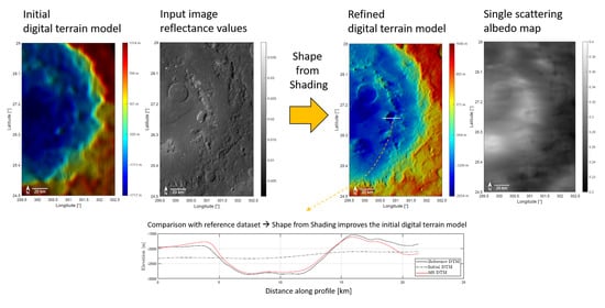
The workflow of the entire 3D reconstruction process of Mercury’s surface is shown in Figure 6. After defining a target area, suitable MDIS images are radiometrically calibrated with ISIS3 [48]. The iterative pyramid scheme begins with the downscaled image and initial DTM, for which we choose one of the stereo DTMs described in Section 1 and Section 2.1. If necessary, the initial DTM is manually co-registered with the calibrated image or mosaic. After estimating the albedo, the SfS algorithm calculates the surface heights. The resulting DTM is used to initialize the next stage. After running through a predefined number of pyramid levels, the resulting DTM and albedo map are of the same resolution as the original image or mosaic. can be used as an initialization for a new run if required.
2.7. Complexity of the Algorithm
To allocate adequate computing resources and to ensure efficient scheduling, the runtime complexity and storage complexity of an algorithm must be known. Therefore, we provide a complexity analysis of our SfS approach with some simplifications. For the sake of argument, we assume rectangular input images of the size pixels.
The SfS procedure of this study falls into three parts: radiometric calibration, co-registration, and our SfS algorithm. For the complexity of stereo reconstruction, which is used for the absolute depth constraint, we refer to the rich literature of stereo algorithms. The input images are radiometrically calibrated by applying the calibration formula to each pixel. Consequently, the complexity of this step becomes . Co-registration is carried out manually, but, as the images grow, more control points are necessary for a robust co-registration. SfS runs N pyramid levels. It starts at the top of the pyramid which means that 3D reconstruction is applied only to a downsized version of the original image. As one descends from the top of the pyramid, the resolution increases by a factor of two at each level until the original resolution of the input image is met. As described by Grumpe et al. [43] and Grumpe and Wöhler [10], the 3D-reconstruction of each pyramid level runs two nested loops. The number of iterations until the reconstruction converges is not a function of the image’s input size but highly depends on the specific surface under investigation and the parameter settings of the weights. Therefore, the number of iterations is generally hard to predict. Experience from this study and previous studies [10,11,43] showed that the routine usually converges within 100–1000 iterations. Consequently, the runtime complexity of the ith level is
Given the number of N pyramid levels, the total complexity becomes
In practice, the last pyramid level is by far the most dominant contributor to runtime. On a Desktop PC with an Intel i7 processor, a region of pixels will take between several minutes and several hours until convergence. If one opts for the iterative albedo retrieval, as described in Section 2.5, the whole procedure has to be carried out multiple times which is only recommended for specific sites with unusually high albedo contrast. Because 3D-reconstruction is usually applied to a manageable number of target sites and without real-time constraints, it can be run over night. Larger mapping campaigns would benefit from parallelization, which is possible and has been applied in the past. The algorithm needs at least the image, the height map, the gradient map, and the albedo map in the storage such that the memory complexity becomes .
2.8. Evaluation Methods
The evaluation of high-resolution DTMs of Mercury is challenging. No actual ground truth (GT) has ever been acquired on Mercury’s surface directly. A viable surrogate is to compare the SfS DTMs against other reference datasets that are available for the planet. In the literature, the SfS results are commonly compared with laser altimetry tracks or stereo DTMs. Jiang et al. [16] used points of the Marts Orbiter Altimeter (MOLA [56]) to evaluate SfS DTMs on Mars. Grumpe and Wöhler [10] and Alexandrov and Beyer [12] employed tracks of the Lunar Orbiter Laser Altimeter (LOLA [57]) to evaluate lunar SfS DTMs. SfS DTMs were compared to stereo DTMs by Wu et al. [15]. However, to carry out a meaningful evaluation, the vertical and horizontal accuracy of the reference datasets must be considered.
The vertical deviations between the best stereo reference DTMs available and the MLA tracks are in the range of tens of meters [29], which is similar to the vertical deviation of the SfS DTM but not much less, as it should be when considering the stereo DTMs a GT. Consequently, we do not to ground truth stereo DTMs but rather to reference stereo DTMs, similar to Wu et al. [15]. Nevertheless, stereo DTMs contain a variety of details that are not present in the sparse MLA points, which help to assess the topographic details that are recovered by SfS. The range error (vertical accuracy) of the MLA instrument is less than 1 m [33]. The horizontal resolution of the images that are used for SfS is about tens to hundreds of meters and the vertical accuracy of the DTMs is in a similar range, as we shown in Section 3.3 and Section 3.4. Consequently, the vertical accuracy of the MLA instrument is significantly better than the vertical deviation between the SfS DTMs and MLA data in these cases. This justifies the assumption that MLA points closely approximate the GT (see also [10,43] for DTMs of the Moon).
In theory, the SfS DTMs can achieve a horizontal resolution that comes close to the resolution of the images used [10]. However, due to stereo artifacts, stereo DTMs have an effective resolution that may be about 5–10 times lower than the resolution of the input images [12,13]. Since the images originate from the same dataset, a comparison of larger areas or high-resolution SfS DTMs is not possible directly. For evaluation, the SfS procedure is applied in Section 3.1 and Section 3.2 to low-resolution WAC images of areas where local stereo DTMs are available. This ensures a sufficient difference between the resolution of the SfS DTM and that of the stereo reference DTM, which is required to conduct a meaningful comparison on the same spatial scale. Only the stereo DTMs created by Fassett [29] and discussed in Section 2.1 meet these criteria and are therefore used as reference. The general approach is as follows. First, the SfS DTM and stereo DTM are scaled to the same size. Due to inaccuracies in the camera and image calibration, the DTMs show a shift and must be co-registered manually. The two DTMs are compared qualitatively as well as quantitatively by extracting profiles with distinct surface properties. Due to a vertical offset of several hundred meters caused by the different reference radii, the height of the SfS profile is shifted by minimizing the RMSE. Finally, the RMSE is calculated for the heights and the first derivative along the profiles, as the SfS procedure is particularly suitable for determining surface gradients. We indicate the gradient along the profile by . The viability of this evaluation method is discussed in Section 4.3.
The horizontal resolution of DTMs derived from MLA data and the effective resolution of MLA measurements themselves generally do not match the resolution that SfS can provide. A meaningful evaluation is therefore only possible in a resolution range between MLA footprint size (about 15 to 100 [33]) and distance between sampling points (about 400 [33]). This ensures the assignment of one MLA measurement to roughly one SfS pixel. We chose to directly compare our SfS results to the sampling points instead of comparing them to gridded DTMs derived from MLA data. This ensures that we compare to a measured value instead of an interpolated point. Consequently, SfS DTMs with a resolution between the footprint size and the sampling interval are chosen to carry out the comparison. The MLA tracks and the SfS DTM are co-registered, and a vertical offset may be removed by minimizing the RMSE. Finally, we calculate the RMSE of the height differences and the RMSE of the first derivatives along the track. The limitations of the method are critically discussed in Section 4.3.
3. Results
The evaluation is carried out with areas that are well suited for the evaluation methods described in Section 2.8 and which place different demands on the SfS algorithm. Praxiteles crater (Section 3.1) exhibits strong albedo variations that are counteracted with the iterative albedo estimation. The ghost crater (Section 3.2) and Rachmaninoff basin (Section 3.3) are reconstructed from image mosaics. A tectonic fault (Section 3.4) is chosen to evaluate the performance for input DTMs that are already highly resolved. Additional results of important science targets but with no available reference DTMs are also presented.
3.1. Evaluation Method 1: Praxiteles Crater
The Praxiteles crater has several large depressions at the floor and is therefore classified as a pit-floor crater [29,58]. These pits are marked by their irregular to round shapes, an average size of 10 to 40 , and the absence of raised rims or centers [58,59]. The floors and immediate surroundings of most pit craters are covered by materials that are interpreted as pyroclastic deposits. The adjacent spectral units cause strong contrasts in the albedo, which necessitates the method of initializing the single-scattering albedo, as discussed in Section 2.5. The final albedo map is shown in Figure 7b. Note the high albedo on the inner ring of Praxiteles crater and around the pit on the left side of the image. The image (Figure 7a) used for the SfS algorithm is part of the MDIS-WAC image EW1048451439G and has a resolution of about 250 m/pixel. Because the stereo DTM 301E27N_0 [29] with a nominal resolution of 65 m/pixel is in sinusoidal projection, the WAC image is also projected sinusoidally with a central meridian of . The global stereo DTM [24] was used to initialize the SfS procedure. Table 4 summarizes all properties of the original images and DTMs used for the first evaluation method. In Figure 7c,d, the stereo DTM is compared to the color-coded SfS DTM. The improvements are immediately apparent. Even though the resolution of the image is only about 2.7 times higher than the nominal resolution of the initial DTM, the SfS algorithm successfully reconstructs all large and medium-sized surface features that were unrecognizable before. Even small features that are not visible in the initial stereo DTM, such as craters with a diameter of 1–2 km, can be easily recognized in the SfS DTM.
For quality assessment, the stereo reference DTM is cropped and scaled to the size of the SfS DTM. Due to inaccuracies in the camera and image calibration, as well as the assumed reference radius of Mercury, the DTMs have to be manually co-registered. The final results are shown in Figure 8. Figure 8a,b shows a similar level of detail despite the large difference in nominal resolution of the input data (the reference was generated from NAC, SfS was generated from WAC images). There is, however, a noticeable deviation at the pit crater in the middle of the image. While there is no raised edge in the reference DTM, as expected for this type of depression, a slight height increase of the left crater rim is visible on the reconstructed surface. This indicates that the albedo estimation could not fully model the high reflectance of the deposits on the lower rim. Note, however, that the height and albedo determination is carried out with a single image. The left edge is strongly illuminated because the surface is lit from the south-east. These circumstances make it difficult for the SfS procedure to separate the causes for the high reflectance values. SfS with multiple input images could alleviate this effect as it imposes more constraints to separate height and albedo.
For a more detailed comparison, we chose three profiles (northern, central, and southern) that cut through the pit crater (Figure 8) and plot their elevations (Figure 9a) and derivatives along the profiles (Figure 9b). Figure 9a shows that the largest vertical deviations approximately correspond to the size of a pixel of the SfS DTM and the general shape of the crater was reconstructed well. After shifting the SfS DTM vertically, the final RMSE of each profile is shown in Table 5. In addition to the elevation, the SfS algorithm is also able to accurately determine the first derivative of the surface. We used the same profiles as before and calculated the derivative of the elevation along the profile (Figure 9b). The derivative of the SfS DTM is close to that of the reference DTM.
3.2. Evaluation Method 1: Ghost Crater
The Northern Smooth Plains (NSP), which cover a large part of Mercury’s surface in the higher northern latitudes, are probably of volcanic origin and consist of deposited flood basalts [58]. In contrast to the surrounding terrain, the NSP have a lower density of superimposed craters and are therefore estimated to be younger [60,61]. The NSP can also be spectrally separated from their surroundings by their assignment to the High-Reflective Red Plains (HRP) [62]. Volcanic flooding has partially and sometimes entirely buried many older craters [60]. These ghost craters [61] can be recognized by subtle tectonic features such as wrinkle ridges and graben, which are caused by the local cooling of the lava and the global contraction of Mercury’s surface [63]. Klimczak et al. [64] divided ghost craters into three subtypes, based on the relations between wrinkle ridges and graben. To evaluate the SfS procedure, we choose a crater of the second type [61]. A crater of this type is marked by a nearly circular ridge ring and graben on the inside, especially near the center. Furthermore, its diameter is always more than 40 . The ghost crater used here was already described by Watters et al. [63] and has a diameter of about 100 .
In contrast to the image examined in Section 3.1, the challenge for the SfS method in this case is not the albedo of the surface but the large incidence angles at higher latitudes. Although these circumstances make it easier to identify fine surface features in the ghost crater, the shadows in the superimposed craters impair the reconstruction. The stereo DTM 36E60N_0 [29] with a nominal resolution of 55 m/pixel is chosen for comparison. The resolution of the mosaic of WAC images is about 2.8 times coarser. For the initialization of the SfS procedure, a section of the DLR DTM of the quadrangle H05 [65] is chosen. Contrary to the initial stereo DTM, the SfS algorithm reconstructs the shape of the superimposed craters (see Figure 10a). The graben that run through the ghost crater are also only visible in the SfS DTM (compare the centers of Figure 10a,b). A problem that occurs in both methods is the preferred direction of the reconstruction. In the initial DTM, the crater walls on the eastern and western sides are elevated and indentations are visible on the northern and southern walls. In the SfS DTM, the northern and southern walls are unrealistically elevated instead. In the case of the SfS DTM, this is due to illumination from a south-southwest direction. The use of several images with different illumination conditions could potentially compensate for this effect.
The reference DTM in Figure 11a shows a strip of the region and contains all of the defining features of a ghost crater. The reference DTM gives a better estimate of the three craters at the top of the image, but a part of their interior is missing, which is likely due to faulty block-matching. The SfS method, however, can plausibly reconstruct the interior of the crater using a single image (Figure 11b). The network of graben in the center of the ghost crater is visible in both DTMs. The reference DTM has a noticeably rougher surface than the SfS DTM. The associated limitations of the evaluation are discussed in Section 4.3. In this section, the reference DTM is assumed to be an accurate representation of the surface.
The elevations and derivatives along the northern and the southern profile marked in Figure 11 are shown in Figure 12. The vertical offset of the SfS and initial DTM profiles is adjusted again by minimizing the RMSE. The final RMSE for both, height and derivative along the profile, is given in Table 6. The profiles illustrate the capability of the SfS algorithm to reconstruct surface features, even if they are of a small lateral size. In Figure 11a, the SfS DTM follows the shape of the reference DTM, while the initial DTM does not. Only on the first and last 5 km of the upper profile a deviation is apparent. On the right-hand side, the shape of the surface is estimated correctly, but not the absolute height. In the lower profile, the SfS algorithm modeled the crater very accurately. The derivatives along the profiles (Figure 11b) support this conclusion. The derivative of the southern profile can be seen as correctly reconstructed, considering the difference in resolution. The large proportion of high frequencies complicates the qualitative comparison of the derivatives along the northern profile. However, the low RMSE of indicates good modeling.
3.3. Evaluation Method 2: Rachmaninoff Basin
Rachmaninoff (Figure 13a) is one of the youngest and therefore best preserved peak-ring basins on Mercury [61,66]. The inner ring has a diameter of about 135 and is open on the southern side. The material that makes up the smooth plains in the inner ring can be spectrally assigned to the High-Reflectance Red Plains (HRP). It is probably of volcanic origin and, with an age of one to two billion years old, is interpreted as a trace of recent volcanism on Mercury [66,67]. The plains are crossed by approximately circular graben. These are likely caused by thermal contraction of the cooling volcanic material [68]. Although the basin was flooded with lava, Rachmaninoff contains the lowest elevation on Mercury with below the planet’s global average. The bright spot located southeast between the inner and outer ring is named Suge Facula [69]. Faculae are Red Unit areas on Mercury with particularly high albedo [70]. These are interpreted as pyroclastic deposits, often surrounded by volcanic vents [69]. One of these volcanic vents is located northeast of the Rachmaninoff basin and is examined in Section 3.5.
For the comparison of the SfS DTM with the MLA data, all sample points of the Rachmaninoff crater are selected that have a channel ID of 0, which means they were recorded with the highest threshold for the signal-to-noise ratio [50]. The points are then assigned to their respective tracks and the four MLA tracks with the most points are selected for further investigation. The color-coded SfS DTM is shown in Figure 13b. The positions of the MLA sample points are shown in white. For all tracks, the spacecraft flew across the surface from south to north. The elevation of the SfS DTM is compared to the MLA measurements along the plotted tracks in Figure 14. We also compute the first derivative of the SfS DTM and the MLA points along the track (Figure 15). As mentioned above, uncertainties in the calibration of the instruments lead to small deviations in the calculated positions. Therefore, co-registration of the data is advised. This is achieved by correcting the lateral shift and the vertical offset by minimizing the RMSE. The final RMSE for each track is given in Table 7. Overall, the MLA data and the reconstructed surface elevation show a good fit and the RMSE of the elevations improved for every track compared to the initial stereo DTM. As shown in Figure 13b, the SfS algorithm estimates the lowest point to be at . The deviation of approximately 300 to the actual minimum can be explained by the fact that the determination of absolute depth in the SfS procedure strongly depends on the initial DTM. For the reconstruction the global DTM of Becker et al. [24] was chosen, with a minimum at .
In many situations, SfS can plausibly recreate the derivative of the surface as for example in Figure 15b between sampling points 300–400 and 500–600. The stereo profile is smooth, but SfS gradually aligns with the derivatives of the MLA track. Considering the RMSE of the along track derivatives, SfS is better in three out of four cases. For the outer western track, the RMSE values of the derivatives can be considered equal, but no improvement is evident. Even though all profiles followed the same co-registration procedure, the SfS derivatives in Figure 15a between sampling points 500 and 600 appear to be shifted. This likely worsens the RMSE. Figure 15 generally shows that the first derivative of the MLA track exhibits stronger amplitudes compared to the SfS or the stereo DTM.
3.4. Evaluation Method 2: Tectonic Fault
The fault that runs through the heavily eroded crater in the center of WAC image EW1014041070G (Figure 16a) is a sign of Mercury’s rich tectonic activity. This shortening structure [5] is probably a lobate scarp [71], which is characterized by its asymmetrical shape. The western side of the scarp has a defined and steep edge, while the slope on the other side is much less pronounced [5,72] (white arrows in Figure 16b). The cause of the shortening structure is likely the global contraction resulting from internal cooling [73]. Along with impact events and volcanic activity, tectonics contributed significantly to the formation of Mercury’s surface. We created a SfS DTM (Figure 16b) that covers this representative region with a resolution of the input image of 178 m/pixel. The resolution of the initial stereo DTM is 222 m/px.
Again, the elevation of the SfS DTM and the initial stereo DTM are compared to MLA measurements along the tracks that are shown in Figure 14. To adjust the MLA tracks and the DTMs, the lateral shift and the vertical offset are corrected by minimizing the RMSE. Furthermore, the first derivative is determined in the direction of the MLA tracks. The final RMSEs of the elevation error and the error of the along track derivatives are given in Table 8. For the inner western track, the RMSE of the SfS DTM is clearly better than the RMSE of the initial stereo DTM. The plot of the elevation profile shows that small details are better retrieved with the SfS algorithm (Figure 17b). In two cases, the RMSE values are rather similar. Given the resolution of the image with 178 m/pixel, we do not consider these RMSE differences as a clear indication that either SfS or stereo is better than the other method. For the outer easter MLA track, the RMSE of the SfS DTM is worse compared to the initial stereo DTM. In that case, the RMSE increased because the bottom of the crater between sampling points 30 and 50 deviates from the MLA track (Figure 17d). This can either arise from a wrong reconstruction because the crater is nearly in shadow impairing the SfS or from a misalignment between height profiles. The RMSE of the along track derivatives clearly improved in three of four cases (see Figure 18b–d). In one case (outer western track, Figure 18a), the improvement can not be considered significant. Again, there is a small crater that is partly shadowed, which may worsen the RMSE of the along track derivative.
3.5. Nathair Facula
Nathair Facula is the most extensive accumulation of Red Unit material on Mercury [62,69]. During the MESSENGER mission, the spot received great interest and became a dedicated science target. Several high-resolution images were acquired with MDIS-NAC. The highly reflective material is distributed within a radius of 130 around a central vent [6]. Pegg et al. [70] classified the pit with a depth of 4 as one of 64 known compound vents within the 184 faculae discovered on Mercury so far. Wright [67] suggested the subdivision into five eruption centers, which differ in location and time of the eruption, but whose boundaries cannot be separated as clearly as in other compounds vents. The earliest eruption took place in the southeast corner of the pit. The present smooth and uniform surface was formed by the flowing material of eruptions that occurred later on. The most recent eruption took place in the northern part, evident by the much rougher structure of the ground and further small depressions [67,70]. These characteristics are reconstructed very well in the SfS DTM (Figure 19b). Although the stitching of the mosaic is not optimal, the method produces a DTM with enhanced details. Even details of small lateral extent, such as small craters superimposed on the smooth plains in the southeast, can be seen in the reconstruction. The fan-shaped walls of the vent, interpreted as a sign of downslope mass movement by Malliband et al. [74], are also visible. The rendered representation of the compound vent (Figure 19b), in conjunction with the color-coded DTM, shows that the wall on the south-eastern side has a much more gentle slope and does not exhibit the fan-like structure of the northern and western walls. Although the resolution of the mosaic at 30 m/pixel is relatively high for Mercury, it is not sufficient to resolve the hollows on the walls identified by Blewett et al. [55].
3.6. Hollows
The characteristics and the formation process of hollows are discussed in Section 2.5. In this section, we present the first high resolution DTMs of these unique surface features.
The mosaic in Figure 20a was already examined by Blewett et al. [55]. They proposed a formation and aging sequence for hollows, in which growing hollows are characterized by their high albedo. Eventually, the hollows stop to become wider and lose their bright halo until they are finally eroded by space weathering [55,75,76]. SfS enables the reconstruction of surface features this small in size, of which only single targeted images are available. The innovations introduced in Section 2.5 are able to compensate the strong albedo effects in Figure 20a. The global stereo DTM [24] was used to initialize the SfS algorithm. The resulting DTM is shown in Figure 20b at a resolution of 15.3 m/pixel. Blewett et al. [55] noticed that hollows are often located on steep crater walls and central peaks (Figure 20b and Figure A2). The hollows are located slightly offset from the ridge of the crater ring on the Sun-facing side. Blewett et al. [55] suspected that the Sun heating the surface could contribute to the formation of hollows.
The hollows shown in Figure 21a at a resolution of 3.3 m/pixel are located on a small hill at the inner crater rim of the heavily eroded Sholem Aleichem impact basin [77]. The sudden transition from the flat floor to the straight wall, visible in the image and the SfS DTM (Figure 21b), distinguishes hollows from other types of small depressions [76]. No superimposed craters are visible inside the hollows. The smallest craters which are recognizable at this resolution are located on the outside. The dots visible on the floors of the hollows are not impact craters, but probably residues of old surface material. Figure A3 shows the rendered SfS DTM.
4. Discussion
To adapt the SfS algorithm to Mercury and MDIS image data, we introduced two innovations. The DTMs that were created with the expanded SfS algorithm and evaluated in Section 3 are discussed in Section 4.1. The viability of the methods and future work are reviewed in Section 4.2. As already mentioned in Section 2.8, the evaluation of SfS DTMs is challenging. We approached this task by comparing our results with two different datasets, i.e., stereo images and laser altimetry data. However, the evaluation methods pose several issues that we discuss in Section 4.3.
4.1. Results of SfS
We compared the SfS DTMs with MLA tracks that approximate the GT and with stereo reference DTMs. For Praxiteles crater (Section 3.1), the ghost crater (Section 3.2), and Rachmaninoff basin (Section 3.3), a large resolution gap between the initial DTM and the image exists, and the SfS algorithm significantly improves the initial DTM. Figure 9a,b and Figure 12a,b indicate that the height and slopes all improve well. We found that the elevation RMSE of the reconstructed Praxiteles crater and the ghost crater lies in the range of 20.05 to 120.00 , and the RMSE of the derivative along the profile is in the range of 0.025–0.062. The deviations in height are smaller than the horizontal resolution of the original images, which are 250 m/pixel for Praxiteles, and 155 m/pixel for the ghost crater. Furthermore, the results in Section 3.3 show that the reconstruction of the Rachmaninoff crater yields an improved RMSE toward MLA tracks compared to the initial stereo DTM (see Table 7). The RMSE of the derivative along the MLA track also improved in three of four cases.
For the fault line (Section 3.4), the resolution difference between the initial DTM and the image is small, and the RMSE of the absolute heights remains in the range of the RMSE of the initial stereo DTM (Section 3.4 and Table 8). However, the RMSE of the derivative along the track improves. This aligns with the results from Hess et al. [11] and is further underpinned by the visual impression that the SfS DTMs appear sharper and more details are visible (see Figure 8b, Figure 11, Figure 16b, Figure 19b, Figure 20b, and Figure 21b). The improved slopes are relevant for any study that involves surface roughness, thermal modeling, analysis of fine structures, and hazard assessment for landers. We also found that very dark regions may impact the SfS result. The two MLA profiles in Figure 17a,d intersect crater-walls that are nearly shadowed, which increased the RMSE of these profiles. The DTMs presented in this article are available in the Supplementary Material.
4.2. Viability of the Novel Methods
The ghost crater and the Rachmaninoff basin were reconstructed from image mosaics, and the Praxiteles crater was reconstructed with our iterative albedo estimation. From the results, we conclude that the SfS routine that is modified by both methods can successfully retrieve the shapes that are present in the reference stereo DTMs. However, both extensions require a critical discussion.
The first innovation we introduced is a way to apply SfS to mosaics of MDIS images, which consist of tiles with considerably different lighting and observation conditions. This method became necessary because many target areas comprise several images that were taken at various times. Because the phase function of the Hapke [17] reflectance model, with the global parameters of Warell [44], was not able to model the reflectance transitions at the image borders adequately, the albedo determination had to be adjusted. By separately estimating the single-scattering albedo for each image of the mosaic, the reflectance variations are absorbed, and realistic DTMs can be produced. However, this method leads to visible discontinuities in the albedo, which are not necessarily physically justified. A further step may be introduced in the future to make the approach more physically plausible by estimating the parameters b and c of the DHG phase function for the entire mosaic until the albedo is continuous at the image boundaries.
The second innovation refers to the effect that some surface features such as pit craters, hollows or volcanic vents have on the albedo. The strong local and topographically correlated albedo variations could not be correctly estimated before. This resulted in inaccurate slope and elevation calculations. To solve this problem, an iterative process was introduced in which the final albedo map is used as initialization for a new SfS run. Usually, only a few iterations were necessary to significantly increase the quality of the final DTM. Additional image processing techniques such as segmentation of bright spots may improve the albedo estimation further.
4.3. Limitations of the Evaluation Methods
In Section 3.1 and Section 3.2, the stereo DTMs of Fassett [29] are used as reference DTMs, because they have the highest horizontal resolution of DTMs available so far. To allow for a direct comparison, the respective reference DTM was scaled down to suppress artifacts known to occur in stereo DTMs [11]. However, there must be a sufficiently large gap between the nominal resolutions of the reference DTMs and SfS DTMs to make sure that no stereo artifacts impede the evaluation. In Section 3.1, the nominal resolution of the original image used in the SfS process is coarser than the nominal resolution of the reference DTM by a factor of 3.9 (reference: 65 m/pixel; WAC image: 250 m/pixel). Note that Fassett [29] already specified the stereo DTMs as three times coarser than the resolution of the MDIS images that were used for stereo. Consequently, there is a significant gap (11.7) between the nominal resolution of the NAC images used for the stereo DTM and the WAC image that is used for SfS. In Section 3.2, the overall factor is 8.4 (reference: 55 m/pixel; WAC image: 155 m/pixel). We examined the limitations of this approach and rendered profiles sampled from Figure 11 and compared them to their respective original images (Figure 22). All DTMs were artificially illuminated from the same direction as the corresponding original images which are shown next to them as reference. The NAC image is an orthoimage created by Fassett [29] from the stereo image pairs. The WAC image data are extracted from the mosaic, which is the basis for the SfS DTM (Figure 11b). On the one hand, the stereo DTM is covered by a pattern of high-frequency diagonal structures that are not present in the original MDIS images. In Figure 22, the impression arises that the SfS DTM represents the surface more precisely, because the rendered SfS DTM and the WAC image match. On the other hand, the stereo DTM more convincingly represents some surface features, such as the graben on the right hand side of the image and the elevation west of the crater. Consequently, it can be seen that there are still stereo artifacts in the reference DTM and the resolution gap is somewhat small. A direct comparison between the stereo reference DTM and SfS DTM has to be extended by considering the local context of absolute height data and surface plausibility. Regardless, it is remarkable that the SfS was constructed from the low resolution WAC image and largely agrees with the stereo data that were derived from the NAC images of much higher resolution.
The evaluation with MLA data has the same basic problem as the comparison with stereo reference DTMs on Mercury. The resolution of DTMs derived from MLA data and the effective resolution of individual MLA measurements generally do not match the resolution that SfS can provide. The SfS DTM at 255 m/pixel in Section 3.3 and the SfS DTM at 178 m/pixel in Section 3.4 were specifically created for this evaluation and fit the criteria we establish in Section 2.8. The results suggest that SfS generally compares well to MLA tracks. However, in the case of Rachmaninoff, we found that the amplitude of the derivatives of the MLA track are stronger compared to the SfS DTM and the stereo DTM (Figure 15). This is not the case for the tectonic fault (Figure 18) where the amplitudes of the MLA derivatives and SfS derivatives are much more alike. A potential explanation could be the different resolution of the input images. The images of the Rachmaninoff crater have a coarser resolution, which may, in fact, yield SfS DTMs that are too coarse for comparing the derivatives with MLA tracks. For the tectonic fault, the scales match, which allows for a direct comparison.
Furthermore, the RMSE or derived quantities are a common choice for comparison, but it comes with limitations. If there is one surface feature that deviates from the reference, it worsens the results even if the rest of the DTM is perfect. Because no actual ground truth of Mercury has ever been acquired, the RMSE values between the SfS DTMs and the approximative GT or reference DTMs are good performance measures but no absolute truth. All these limitations have to be kept in mind when interpreting the RMSE values of the elevation or the derivatives. Therefore, we emphasize that it is necessary to consider the context of the DTM and compare the SfS results with different datasets to arrive at a comprehensive picture of what SfS can provide.
5. Conclusions
We adapted the SfS algorithm of Grumpe and Wöhler [10] and used it to generate digital terrain models of Mercury’s surface. The challenges posed by the properties of the surface and the available datasets lead to the introduction of two methodical innovations. Seamless mosaic shading and iterative albedo estimation were proven to work on Mercury. We found that these innovations can overcome the challenges that are introduced by the sparsely available imagery of Mercury, the comparatively small image patches that require mosaicking, and the brightness variations of the planet’s unique surface features. The selection of the areas investigated in this paper served primarily to evaluate and demonstrate the capabilities of the SfS procedure. We confirmed that SfS is well suited to retrieve the shape of the surface by creating accurate heights and derivatives. If the initial stereo DTM is already well resolved, SfS could not improve the RMSE of the absolute heights, but the DTM is sharpened such that the derivatives became more accurate. Furthermore, we presented improved DTMs of Mercury’s unique science targets and were the first to compute DTMs with 3.3 m/pixel of Hollows.
Supplementary Materials
The SfS DTMs constructed in this work are available online at https://0-www-mdpi-com.brum.beds.ac.uk/2072-4292/12/23/3989/s1.
Author Contributions
Conceptualization, M.T. and K.W.; methodology, M.T and K.W; software, M.T.; validation, K.W. and C.W.; resources, C.W.; data curation, M.T.; writing—original draft preparation, M.T. and K.W.; writing—review and editing, M.T., K.W. and C.W.; visualization, M.T.; and supervision, K.W. and C.W. All authors have read and agreed to the published version of the manuscript.
Funding
This research received no external funding.
Conflicts of Interest
The authors declare no conflict of interest.
Appendix A
Figure A1.
Illumination geometry. The normal of a surface element is . The vector points to the light source and spans the angle of incidence i with . points towards the observer with the emission angle e. The angle between and is the phase angle .
Figure A1.
Illumination geometry. The normal of a surface element is . The vector points to the light source and spans the angle of incidence i with . points towards the observer with the emission angle e. The angle between and is the phase angle .

Figure A2.
Rendered SfS DTM. For illustration purposes, the z-axis is multiplied by a factor of 2.

Figure A3.
Rendered SfS DTM.

References
- Solomon, S.C.; Anderson, B.J. The MESSENGER Mission: Science and Implementation Overview. In Mercury: The View after MESSENGER; Cambridge Planetary Science, Cambridge University Press: Cambridge, UK, 2018; pp. 1–29. [Google Scholar] [CrossRef]
- McNutt, R.L., Jr.; Benkhoff, J.; Fujimoto, M.; Anderson, B.J. Future Missions: Mercury after MESSENGER. In Mercury: The View after MESSENGER; Cambridge Planetary Science, Cambridge University Press: Cambridge, UK, 2018; pp. 544–569. [Google Scholar] [CrossRef]
- Solomon, S.C.; Nittler, L.R.; Anderson, B.J. Mercury: The View after MESSENGER; Cambridge Planetary Science, Cambridge University Press: Cambridge, UK, 2018. [Google Scholar] [CrossRef]
- Steiger, C.; Montagnon, E.; Accomazzo, A.; Ferri, P. BepiColombo mission to Mercury: First year of flight. Acta Astronaut. 2020, 170, 472–479. [Google Scholar] [CrossRef]
- Byrne, P.K.; Klimczak, C.; Sengör, C. The Tectonic Character of Mercury. In Mercury: The View after MESSENGER; Cambridge Planetary Science, Cambridge University Press: Cambridge, UK, 2018; pp. 249–286. [Google Scholar] [CrossRef]
- Thomas, R.J.; Rothery, D.A. Volcanism on Mercury. Elements 2019, 15, 27–32. [Google Scholar] [CrossRef]
- Hiesinger, H.; Helbert, J.; Team, M.C.I. The Mercury radiometer and thermal infrared spectrometer (MERTIS) for the BepiColombo mission. Planet. Space Sci. 2010, 58, 144–165. [Google Scholar] [CrossRef]
- Hawkins, S.E.; Boldt, J.D.; Darlington, E.H.; Espiritu, R.; Gold, R.E.; Gotwols, B.; Grey, M.P.; Hash, C.D.; Hayes, J.R.; Jaskulek, S.E.; et al. The Mercury dual imaging system on the MESSENGER spacecraft. Space Sci. Rev. 2007, 131, 247–338. [Google Scholar] [CrossRef]
- Flamini, E.; Capaccioni, F.; Colangeli, L.; Cremonese, G.; Doressoundiram, A.; Josset, J.; Langevin, Y.; Debei, S.; Capria, M.; De Sanctis, M.; et al. SIMBIO-SYS: The spectrometer and imagers integrated observatory system for the BepiColombo planetary orbiter. Planet. Space Sci. 2010, 58, 125–143. [Google Scholar] [CrossRef]
- Grumpe, A.; Wöhler, C. Recovery of elevation from estimated gradient fields constrained by digital elevation maps of lower lateral resolution. ISPRS J. Photogramm. Remote Sens. 2014, 94, 37–54. [Google Scholar] [CrossRef]
- Hess, M.; Wohlfarth, K.; Grumpe, A.; Wöhler, C.; Ruesch, O.; Wu, B. Atmospherically compensated Shape from Shading on the Martian surface: Towards the perfect digital terrain model of Mars. Int. Arch. Photogramm. Remote. Sens. Spat. Inf. Sci. 2019, XLII-2/W13, 1405–1411. [Google Scholar] [CrossRef] [Green Version]
- Alexandrov, O.; Beyer, R.A. Multiview Shape-From-Shading for Planetary Images. Earth Space Sci. 2018, 5, 652–666. [Google Scholar] [CrossRef]
- Gehrig, S.; Franke, U. Stereovision for ADAS. In Handbook of Driver Assistance Systems; Winner, H., Hakuli, S., Lotz, F., Singer, C., Eds.; Springer International Publishing: Cham, Switzerland, 2016; pp. 495–524. [Google Scholar]
- Horn, B.K. Height and gradient from shading. Int. J. Comput. Vis. 1990, 5, 37–75. [Google Scholar] [CrossRef]
- Wu, B.; Liu, W.C.; Grumpe, A.; Wöhler, C. Construction of pixel-level resolution DEMs from monocular images by shape and albedo from shading constrained with low-resolution DEM. ISPRS J. Photogramm. Remote Sens. 2018, 140, 3–19. [Google Scholar] [CrossRef]
- Jiang, C.; Douté, S.; Luo, B.; Zhang, L. Fusion of photogrammetric and photoclinometric information for high-resolution DEMs from Mars in-orbit imagery. ISPRS J. Photogramm. Remote Sens. 2017, 130, 418–430. [Google Scholar] [CrossRef]
- Hapke, B. Theory of Reflectance and Emittance Spectroscopy; Cambridge University Press: Cambridge, UK, 2012. [Google Scholar]
- Van Diggelen, J. A photometric investigation of the slopes and the heights of the ranges of hills in the Maria of the moon. Bull. Astron. Institutes Neth. 1951, 11, 283. [Google Scholar]
- Rindfleisch, T. A photometric method for deriving lunar topographic information. In JPL Technical Report N. 32–786; Jet Propulsion Laboratory: Pasadena, CA, USA, 1965. [Google Scholar]
- Hapke, B.; Danielson, G.E.; Klaasen, K.; Wilson, L. Photometric observations of Mercury from Mariner 10. J. Geophys. Res. 1975, 80, 2431–2443. [Google Scholar] [CrossRef]
- Mouginis-Mark, P.J.; Wilson, L. Photoclinometric measurements of Mercurian landforms. Lunar Planet. Sci. Conf. 1979, 10, 873–875. [Google Scholar]
- Mouginis-Mark, P.J.; Wilson, L. MERC: A FORTRAN IV program for the production of topographic data for the planet Mercury. Comput. Geosci. 1981, 7, 35–45. [Google Scholar] [CrossRef]
- Watters, T.; Robinson, M.; Cook, A. Topographic models for Discovery Rupes, Mercury using digital stereophotogrammetry and photoclinometry. Lunar Planet. Sci. Conf. 1997, 28, 509. [Google Scholar]
- Becker, K.; Robinson, M.; Becker, T.; Weller, L.; Edmundson, K.; Neumann, G.; Perry, M.; Solomon, S. First global digital elevation model of Mercury. Lunar Planet. Sci. Conf. 2016, 47, 2959. [Google Scholar]
- Becker, K.; Berry, K.; Mapel, J.; Walldren, J. A new approach to create image control networks in ISIS. In Proceedings of the Third Planetary Data Workshop and The Planetary Geologic Mappers Annual Meeting, Flagstaff, AZ, USA, 12–15 June 2017; Volume 1986. [Google Scholar]
- Denevi, B.W.; Chabot, N.L.; Murchie, S.L.; Becker, K.J.; Blewett, D.T.; Domingue, D.L.; Ernst, C.M.; Hash, C.D.; Hawkins, S.E.; Keller, M.R.; et al. Calibration, projection, and final image products of MESSENGER’s Mercury Dual Imaging System. Space Sci. Rev. 2018, 214, 2. [Google Scholar] [CrossRef]
- Preusker, F.; Oberst, J.; Stark, A.; Burmeister, S. Mercury stereo topographic mapping using data from the MESSENGER orbital mission. In Planetary Remote Sensing and Mapping; CRC Press: Boca Raton, FL, USA, 2018; pp. 167–180. [Google Scholar]
- Batson, R.M.; Greeley, R. Planetary Mapping; Cambridge University Press: Cambridge, UK, 1990. [Google Scholar]
- Fassett, C.I. Ames stereo pipeline-derived digital terrain models of Mercury from MESSENGER stereo imaging. Planet. Space Sci. 2016, 134, 19–28. [Google Scholar] [CrossRef] [Green Version]
- Beyer, R.A.; Alexandrov, O.; McMichael, S. The Ames Stereo Pipeline: NASA’s open source software for deriving and processing terrain data. Earth Space Sci. 2018, 5, 537–548. [Google Scholar] [CrossRef]
- Henriksen, M.; Manheim, M.; Becker, K.; Howington-Kraus, E.; Robinson, M. High Resolution Regional Digital Terrain Models and Derived Products from MESSENGER MDIS Images. In Proceedings of the Second Planetary Data Workshop, Flagstaff, AZ, USA, 8–11 June 2015; Volume 1846. [Google Scholar]
- Manheim, M.; Henriksen, M.; Robinson, M.; Team, M. High-resolution local-area digital elevation models and derived products for Mercury from MESSENGER images. In Proceedings of the Third Planetary Data Workshop and The Planetary Geologic Mappers Annual Meeting, Flagstaff, AZ, USA, 12–15 June 2017; Volume 1986. [Google Scholar]
- Zuber, M.T.; Smith, D.E.; Phillips, R.J.; Solomon, S.C.; Neumann, G.A.; Hauck, S.A.; Peale, S.J.; Barnouin, O.S.; Head, J.W.; Johnson, C.L.; et al. Topography of the northern hemisphere of Mercury from MESSENGER laser altimetry. Science 2012, 336, 217–220. [Google Scholar] [CrossRef] [PubMed] [Green Version]
- Kirk, R. A Fast Finite-Element Algorithm for Two-Dimensional Photoclinometry. Ph. D. Thesis, Division of Geological and Planetary Sciences, California Institute of Technology, Pasadena, CA, USA, 1987. [Google Scholar]
- Kirk, R.L.; Howington-Kraus, E.; Redding, B.; Galuszka, D.; Hare, T.M.; Archinal, B.A.; Soderblom, L.A.; Barrett, J.M. High-resolution topomapping of candidate MER landing sites with Mars Orbiter Camera narrow-angle images. J. Geophys. Res. Planets 2003, 108. [Google Scholar] [CrossRef]
- Shao, M.; Chellappa, R.; Simchony, T. Reconstructing a 3-D depth map from one or more images. Image Underst. 1991, 53, 219–226. [Google Scholar] [CrossRef]
- Liu, W.C.; Wu, B. An integrated photogrammetric and photoclinometric approach for illumination-invariant pixel-resolution 3D mapping of the lunar surface. ISPRS J. Photogramm. Remote Sens. 2020, 159, 153–168. [Google Scholar] [CrossRef]
- Douté, S.; Jiang, C. Small-Scale Topographical Characterization of the Martian Surface With In-Orbit Imagery. IEEE Trans. Geosci. Remote Sens. 2019, 58, 447–460. [Google Scholar] [CrossRef]
- Shkuratov, Y.; Starukhina, L.; Hoffmann, H.; Arnold, G. A model of spectral albedo of particulate surfaces: Implications for optical properties of the Moon. Icarus 1999, 137, 235–246. [Google Scholar] [CrossRef]
- McEwen, A.S. Photometric functions for photoclinometry and other applications. Icarus 1991, 92, 298–311. [Google Scholar] [CrossRef]
- Ceamanos, X.; Douté, S.; Fernando, J.; Schmidt, F.; Pinet, P.; Lyapustin, A. Surface reflectance of Mars observed by CRISM/MRO: 1. Multi-angle Approach for Retrieval of Surface Reflectance from CRISM observations (MARS-ReCO). J. Geophys. Res. Planets 2013, 118, 514–533. [Google Scholar] [CrossRef] [Green Version]
- Kirk, R.L.; Barrett, J.M.; Soderblom, L.A. Photoclinometry made simple...? In Proceedings of the ISPRS Working Group IV/9 Workshop “Advances in Planetary Mapping 2003”, Houston, TX, USA, 22 March 2003. [Google Scholar]
- Grumpe, A.; Belkhir, F.; Wöhler, C. Construction of lunar DEMs based on reflectance modelling. Adv. Space Res. 2014, 53, 1735–1767. [Google Scholar] [CrossRef]
- Warell, J. Properties of the Hermean regolith: IV. Photometric parameters of Mercury and the Moon contrasted with Hapke modelling. Icarus 2004, 167, 271–286. [Google Scholar] [CrossRef]
- Hapke, B. Bidirectional reflectance spectroscopy: 5. The coherent backscatter opposition effect and anisotropic scattering. Icarus 2002, 157, 523–534. [Google Scholar] [CrossRef] [Green Version]
- Gold, R.E.; Solomon, S.C.; McNutt, R.L., Jr.; Santo, A.G.; Abshire, J.B.; Acu na, M.H.; Afzal, R.S.; Anderson, B.J.; Andrews, G.B.; Bedini, P.D.; et al. The MESSENGER mission to Mercury: Scientific payload. Planet. Space Sci. 2001, 49, 1467–1479. [Google Scholar] [CrossRef]
- Gaddis, L.; Anderson, J.; Becker, K.; Becker, T.; Cook, D.; Edwards, K.; Eliason, E.; Hare, T.; Kieffer, H.; Lee, E.; et al. An overview of the integrated software for imaging spectrometers (ISIS). Lunar Planet. Sci. Conf. 1997, 28, 387. [Google Scholar]
- Anderson, J.; Sides, S.; Soltesz, D.; Sucharski, T.; Becker, K. Modernization of the Integrated Software for Imagers and Spectrometers. In Proceedings of the 35th Lunar and Planetary Science Conference, League City, TX, USA, 15–19 March 2004. [Google Scholar]
- Becker, K.J.; Anderson, J.A.; Weller, L.A.; Becker, T.L. ISIS support for NASA mission instrument ground data processing systems. Lunar Planet. Sci. Conf. 2013, 44, 2829. [Google Scholar]
- Neumann, G. MESSENGER: Software Interface Specification For The Mercury Laser Altimeter Calibrated, Reduced and Gridded Data Records; Code 698; NASA Goddard Space Flight Center: Greenbelt, MD, USA, 2017.
- McAdams, J.V.; Bryan, C.G.; Moessner, D.P.; Page, B.R.; Stanbridge, D.R.; Williams, K.E. Orbit design and navigation through the end of MESSENGER’s extended mission at Mercury. In Proceedings of the 24th Space Flight Mechanics Meeting, American Astronautical Society/American Institute of Aeronautics and Astronautics, Santa Fe, NM, USA, 26–30 January 2014; pp. 14–369. [Google Scholar]
- Cavanaugh, J.F.; Smith, J.C.; Sun, X.; Bartels, A.E.; Ramos-Izquierdo, L.; Krebs, D.J.; McGarry, J.F.; Trunzo, R.; Novo-Gradac, A.M.; Britt, J.L.; et al. The Mercury Laser Altimeter instrument for the MESSENGER mission. Space Sci. Rev. 2007, 131, 451–479. [Google Scholar] [CrossRef] [Green Version]
- Domingue, D.L.; Denevi, B.W.; Murchie, S.L.; Hash, C.D. Application of multiple photometric models to disk-resolved measurements of Mercury’s surface: Insights into Mercury’s regolith characteristics. Icarus 2016, 268, 172–203. [Google Scholar] [CrossRef] [Green Version]
- Shkuratov, Y.; Kaydash, V.; Korokhin, V.; Velikodsky, Y.; Opanasenko, N.; Videen, G. Optical measurements of the Moon as a tool to study its surface. Planet. Space Sci. 2011, 59, 1326–1371. [Google Scholar] [CrossRef]
- Blewett, D.T.; Ernst, C.M.; Murchie, S.L.; Vilas, F. Mercury’s Hollows. In Mercury: The View after MESSENGER; Cambridge Planetary Science, Cambridge University Press: Cambridge, UK, 2018; pp. 324–345. [Google Scholar] [CrossRef]
- Zuber, M.T.; Smith, D.E.; Solomon, S.C.; Muhleman, D.O.; Head, J.W.; Garvin, J.B.; Abshire, J.B.; Bufton, J.L. The Mars Observer laser altimeter investigation. J. Geophys. Res. Planets 1992, 97, 7781–7797. [Google Scholar] [CrossRef]
- Riris, H.; Cavanaugh, J.; Sun, X.; Liiva, P.; Rodriguez, M.; Neuman, G. The Lunar Orbiter Laser Altimeter (LOLA) on NASA’s Lunar Reconnaissance Orbiter (LRO) mission. In Proceedings of the International Conference on Space Optics, Rhodes, Greece, 4–8 October 2010; Armandillo, E., Cugny, B., Karafolas, N., Eds.; International Society for Optics and Photonics. SPIE: Bellingham, WA, USA, 2010; Volume 10565, pp. 93–98. [Google Scholar]
- Byrne, P.K.; Whitten, J.L.; Klimczak, C.; Mccubbin, F.M.; Ostrach, L.R. The Volcanic Character of Mercury. In Mercury: The View after MESSENGER; Cambridge Planetary Science, Cambridge University Press: Cambridge, UK, 2018; pp. 287–323. [Google Scholar] [CrossRef]
- Gillis-Davis, J.J.; Blewett, D.T.; Gaskell, R.W.; Denevi, B.W.; Robinson, M.S.; Strom, R.G.; Solomon, S.C.; Sprague, A.L. Pit-floor craters on Mercury: Evidence of near-surface igneous activity. Earth Planet. Sci. Lett. 2009, 285, 243–250. [Google Scholar] [CrossRef]
- Ostrach, L.R.; Robinson, M.S.; Whitten, J.L.; Fassett, C.I.; Strom, R.G.; Head, J.W.; Solomon, S.C. Extent, age, and resurfacing history of the northern smooth plains on Mercury from MESSENGER observations. Icarus 2015, 250, 602–622. [Google Scholar] [CrossRef]
- Chapman, C.R.; Baker, D.M.H.; Barnouin, O.S.; Fasset, C.I.; Marchi, S.; Merline, W.J.; Ostrach, L.R.; Prockter, L.M.; Strom, R.G. Impact Cratering of Mercury. In Mercury: The View after MESSENGER; Cambridge Planetary Science, Cambridge University Press: Cambridge, UK, 2018; pp. 217–248. [Google Scholar] [CrossRef]
- Murchie, S.L.; Klima, R.L.; Izenberg, N.R.; Domingue, D.L.; Blewett, D.T.; Helbert, J. Spectral Reflectance Constraints on the Composition and Evolution of Mercury’s Surface. In Mercury: The View after MESSENGER; Cambridge Planetary Science, Cambridge University Press: Cambridge, UK, 2018; pp. 191–216. [Google Scholar] [CrossRef]
- Watters, T.R.; Solomon, S.C.; Klimczak, C.; Freed, A.M.; Head, J.W.; Ernst, C.M.; Blair, D.M.; Goudge, T.A.; Byrne, P.K. Extension and contraction within volcanically buried impact craters and basins on Mercury. Geology 2012, 40, 1123–1126. [Google Scholar] [CrossRef]
- Klimczak, C.; Watters, T.R.; Ernst, C.M.; Freed, A.M.; Byrne, P.K.; Solomon, S.C.; Blair, D.M.; Head, J.W. Deformation associated with ghost craters and basins in volcanic smooth plains on Mercury: Strain analysis and implications for plains evolution. J. Geophys. Res. Planets 2012, 117. [Google Scholar] [CrossRef]
- Stark, A.; Preusker, F.; Oberst, J.; Matz, K.D.; Gwinner, K.; Roatsch, T. High-Resolution Topography from MESSENGER Orbital Stereo Imaging—The H5 Quadrangle “Hokusai”. In Proceedings of the Lunar and Planetary Science Conference, The Woodlands, TX, USA, 20–24 March 2017; Volume 48. [Google Scholar]
- Prockter, L.M.; Ernst, C.M.; Denevi, B.W.; Chapman, C.R.; Head, J.W.; Fassett, C.I.; Merline, W.J.; Solomon, S.C.; Watters, T.R.; Strom, R.G.; et al. Evidence for young volcanism on Mercury from the third MESSENGER flyby. Science 2010, 329, 668–671. [Google Scholar] [CrossRef] [PubMed] [Green Version]
- Wright, J. MESSENGER Observations of Volcanism on Mercury: From Hokusai Quadrangle Down to Small Cones. Ph.D. Thesis, The Open University, Milton Keynes, UK, 2019. [Google Scholar]
- Blair, D.M.; Freed, A.M.; Byrne, P.K.; Klimczak, C.; Prockter, L.M.; Ernst, C.M.; Solomon, S.C.; Melosh, H.J.; Zuber, M.T. The origin of graben and ridges in Rachmaninoff, Raditladi, and Mozart basins, Mercury. J. Geophys. Res. Planets 2013, 118, 47–58. [Google Scholar] [CrossRef] [Green Version]
- Rothery, D.A. Volcanism on Mercury. In Oxford Research Encyclopedia of Planetary Science; Oxford University Press: Oxford, UK, 2018. [Google Scholar] [CrossRef]
- Pegg, D.; Rothery, D.; Balme, M.; Conway, S. Explosive Vents on Mercury: Commonplace Multiple Eruptions and Their Implications. In Proceedings of the 50th Lunar and Planetary Science Conference 2019, Houston, TX, USA, 18–22 March 2019. [Google Scholar]
- Marchi, S.; Massironi, M.; Cremonese, G.; Martellato, E.; Giacomini, L.; Prockter, L. The effects of the target material properties and layering on the crater chronology: The case of Raditladi and Rachmaninoff basins on Mercury. Planet. Space Sci. 2011, 59, 1968–1980. [Google Scholar] [CrossRef] [Green Version]
- Watters, T.R.; Solomon, S.C.; Robinson, M.S.; Head, J.W.; André, S.L.; Hauck, S.A., II; Murchie, S.L. The tectonics of Mercury: The view after MESSENGER’s first flyby. Earth Planet. Sci. Lett. 2009, 285, 283–296. [Google Scholar] [CrossRef]
- Byrne, P.K.; Klimczak, C.; Şengör, A.C.; Solomon, S.C.; Watters, T.R.; Hauck, S.A. Mercury’s global contraction much greater than earlier estimates. Nat. Geosci. 2014, 7, 301. [Google Scholar] [CrossRef]
- Malliband, C.; Conway, S.; Rothery, D.; Balme, M. Potential Identification of Downslope Mass Movements on Mercury Driven by Volatile-Loss. In Proceedings of the Lunar and Planetary Science Conference, The Woodlands, TX, USA, 18–22 March 2019; Volume 50. [Google Scholar]
- Xiao, Z.; Strom, R.G.; Blewett, D.T.; Byrne, P.K.; Solomon, S.C.; Murchie, S.L.; Sprague, A.L.; Domingue, D.L.; Helbert, J. Dark spots on Mercury: A distinctive low-reflectance material and its relation to hollows. J. Geophys. Res. Planets 2013, 118, 1752–1765. [Google Scholar] [CrossRef] [Green Version]
- Thomas, R.J.; Rothery, D.A.; Conway, S.J.; Anand, M. Hollows on Mercury: Materials and mechanisms involved in their formation. Icarus 2014, 229, 221–235. [Google Scholar] [CrossRef] [Green Version]
- Blewett, D.T.; Stadermann, A.C.; Susorney, H.C.; Ernst, C.M.; Xiao, Z.; Chabot, N.L.; Denevi, B.W.; Murchie, S.L.; McCubbin, F.M.; Kinczyk, M.J.; et al. Analysis of MESSENGER high-resolution images of Mercury’s hollows and implications for hollow formation. J. Geophys. Res. Planets 2016, 121, 1798–1813. [Google Scholar] [CrossRef]
Figure 1.
(a) The mosaic consists of 12 MDIS-NAC images and depicts the inner ring of the Rachmaninoff basin. (b) Albedo map of the inner ring of the Rachmaninoff basin with tile-wise albedo estimation. The boundaries between the individual tiles become more pronounced the more different the lighting conditions are.

Figure 2.
Effects of the old and new albedo estimation on the DTM generated from the mosaic in Figure 1a. (a) The albedo at each pyramid level is calculated for the entire image. The resulting DTM shows strong distortions at the tile boundaries with large differences in reflectance. (b) The albedo is calculated independently for each mosaic tile. No edges are visible at the original image boundaries, resulting in a much more realistic DTM.

Figure 3.
MDIS-NAC image EN0223616383M of Hopper crater. A large part of the floor and the central peak is covered by hollows, easily recognizable by their high reflectance.
Figure 3.
MDIS-NAC image EN0223616383M of Hopper crater. A large part of the floor and the central peak is covered by hollows, easily recognizable by their high reflectance.

Figure 4.
(a) Reconstruction without albedo initialization leads to unrealistic deviations in height left and right of the central peak. (b) The color-coded SfS DTM after the fourth iteration shows a more realistic surface.
Figure 4.
(a) Reconstruction without albedo initialization leads to unrealistic deviations in height left and right of the central peak. (b) The color-coded SfS DTM after the fourth iteration shows a more realistic surface.

Figure 5.
(a) In the first iteration, the process underestimates the albedo of the hollows, which leads to fuzzy borders. (b) After the fourth iteration, the borders are more pronounced and modeled with a higher albedo.
Figure 5.
(a) In the first iteration, the process underestimates the albedo of the hollows, which leads to fuzzy borders. (b) After the fourth iteration, the borders are more pronounced and modeled with a higher albedo.

Figure 6.
SfS workflow adapted from Grumpe et al. [43]. Dashed lines indicate optional steps that are executed if necessary.
Figure 6.
SfS workflow adapted from Grumpe et al. [43]. Dashed lines indicate optional steps that are executed if necessary.

Figure 7.
(a) Part of MDIS-WAC image EW1048451439G which shows the eastern half of Praxiteles crater with bright hollows (yellow arrows) and a bright pit-crater (white arrow) on the inner ring. The strong albedo variations impose a significant challenge to the SfS method. (b) Final albedo map. The high albedo of the hollows and the pit crater are particularly evident as they are much brighter than the outer basin rim. (c) Color-coded initial DTM from Becker et al. [24]. (d) Color-coded SfS DTM.

Figure 8.
(a) The stereo DTM from Fassett [29] that is used for comparison with (b) the SfS DTM. The dashed red lines show the positions of the northern, central and southern profile that are examined in Figure 9.

Figure 9.
(a) Elevation of the northern, central, and southern profile marked in Figure 8. The elevations of the initial DTM (black dotted) and the SfS DTM (red) are compared to the reference DTM (black). (b) First derivative of the reconstructed surface along the same profiles. The along profile derivative of the initial DTM (black dotted) and the SfS DTM (red) are compared to the derivatives of the reference DTM (black). Starting from the low frequency initialization, the SfS algorithm is able to reconstruct the shape of the surface

Figure 10.
(a) Mosaic ofWAC images of the ghost crater at a resolution of 155 m/pixel. (b) Color-coded representation of the SfS DTM.
Figure 10.
(a) Mosaic ofWAC images of the ghost crater at a resolution of 155 m/pixel. (b) Color-coded representation of the SfS DTM.

Figure 11.
Comparison of the (a) reference DTM [29] to the (b) SfS DTM. The profiles indicated by the red dashed lines are investigated in Figure 12 from top to bottom. To allow for the comparison, the stereo DTM is scaled to the size of the SfS DTM.

Figure 12.
(a) Elevation of the northern and southern profile marked in Figure 11. The elevations of the initial DTM (black dotted) and the SfS DTM (red) are compared to the reference DTM (black). (b) First derivative of the reconstructed surface along the same profiles. The derivatives of the initial DTM (black dotted) and the SfS DTM (red) are compared to the derivative of the reference DTM (black).

Figure 13.
(a) Mosaic of WAC images of the Rachmaninoff basin at a resolution of 255 m/pixel. (b) Color-coded representation of the SfS DTM. The MLA sampling points are shown in red. The tracks were always recorded from south to north. The elevations of the individual tracks are compared to the reconstructed surface from left to right in Figure 14.

Figure 14.
Comparison of the MLA tracks (black) to the surface constructed by the SfS procedure (red) and the initial stereo DTM (blue) of the Rachmaninoff basin. The positions of the tracks are given in Figure 13b.
Figure 14.
Comparison of the MLA tracks (black) to the surface constructed by the SfS procedure (red) and the initial stereo DTM (blue) of the Rachmaninoff basin. The positions of the tracks are given in Figure 13b.

Figure 15.
Comparison of the derivative along the MLA tracks (black) to the derivative of the surface constructed by the SfS procedure (red) and the initial stereo DTM (blue) of the Rachmaninoff basin. The positions of the tracks are given in Figure 13b.
Figure 15.
Comparison of the derivative along the MLA tracks (black) to the derivative of the surface constructed by the SfS procedure (red) and the initial stereo DTM (blue) of the Rachmaninoff basin. The positions of the tracks are given in Figure 13b.

Figure 16.
(a) WAC image EW1014041070G shows a fault line through a partially burrowed crater east of the Rachmaninoff basin. (b) Color-coded SfS DTM created from the image. The white lines indicate the position of the MLA profile, the arrows indicate the fault line.
Figure 16.
(a) WAC image EW1014041070G shows a fault line through a partially burrowed crater east of the Rachmaninoff basin. (b) Color-coded SfS DTM created from the image. The white lines indicate the position of the MLA profile, the arrows indicate the fault line.

Figure 17.
Comparison of the MLA tracks (black) to the surface constructed by the SfS procedure (red) and the initial stereo DTM (blue) of the tectonic fault. The positions of the tracks are given in Figure 16b.
Figure 17.
Comparison of the MLA tracks (black) to the surface constructed by the SfS procedure (red) and the initial stereo DTM (blue) of the tectonic fault. The positions of the tracks are given in Figure 16b.

Figure 18.
Comparison of the derivative along the MLA tracks (black) to the derivative of the surface constructed by the SfS procedure (red) and the initial stereo DTM (blue) of the tectonic fault. The positions of the tracks are given in Figure 16b.
Figure 18.
Comparison of the derivative along the MLA tracks (black) to the derivative of the surface constructed by the SfS procedure (red) and the initial stereo DTM (blue) of the tectonic fault. The positions of the tracks are given in Figure 16b.

Figure 19.
(a) Mosaic of the central volcanic vent in the Nathair Facula. The mosaic consists of NAC images and has a resolution of about 30 m/pixel. There are some noticeable georeferencing errors. (b) Color-coded representation of the SfS DTM. The inaccuracies at the mosaic borders were reduced by the process but not completely eliminated. The different surface textures are modeled precisely.

Figure 20.
(a) Mosaic from the NAC images EN0213851669M and EN0213851674M at a resolution of 15.3 m/Pixel. This section of the inner ring of the Aksakov crater shows different stages of the formation of hollows. (b) Color-coded SfS DTM.
Figure 20.
(a) Mosaic from the NAC images EN0213851669M and EN0213851674M at a resolution of 15.3 m/Pixel. This section of the inner ring of the Aksakov crater shows different stages of the formation of hollows. (b) Color-coded SfS DTM.

Figure 21.
(a) NAC image EN1051631967M with a resolution of 3.3m/pixel. (b) Color-coded SfS DTM. The faint streaks running through the DTM parallel to the image borders are caused by artifacts in the original image.
Figure 21.
(a) NAC image EN1051631967M with a resolution of 3.3m/pixel. (b) Color-coded SfS DTM. The faint streaks running through the DTM parallel to the image borders are caused by artifacts in the original image.

Figure 22.
Sections of the DTMs in Figure 11. The DTMs are compared to the corresponding image parts. In the case of the stereo DTM, the original image is an orthophoto from NAC images [29], and, for the SfS DTM, it is the mosaic of WAC images. Below that, the elevation of the profile (red dashed lines) over the length of the section is shown. The SfS DTM is drawn in red and the stereo DTM in black.


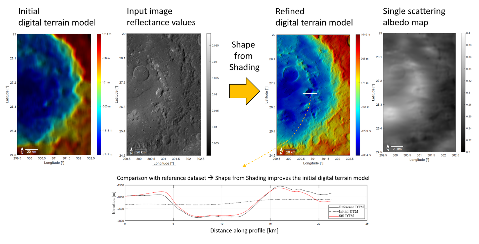
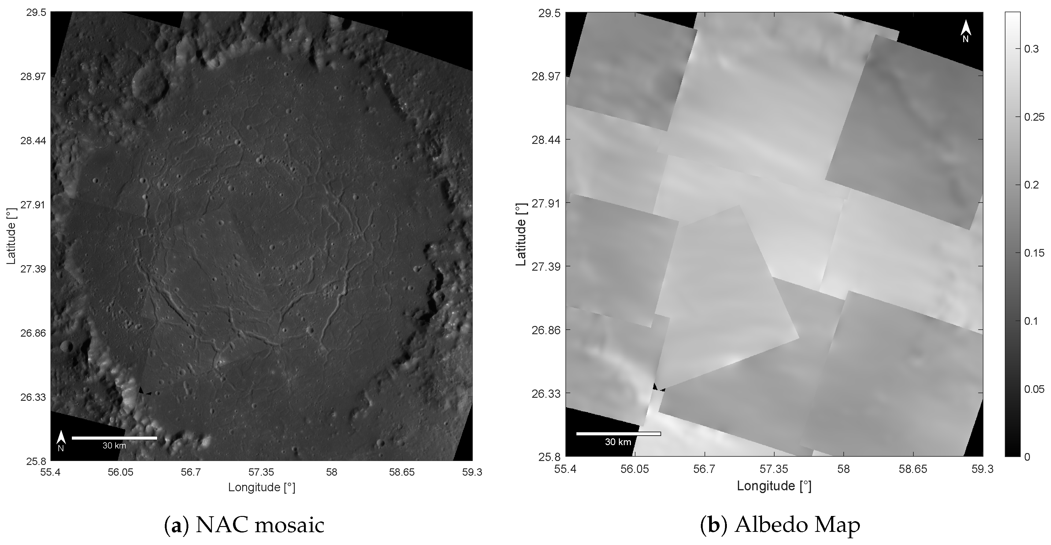
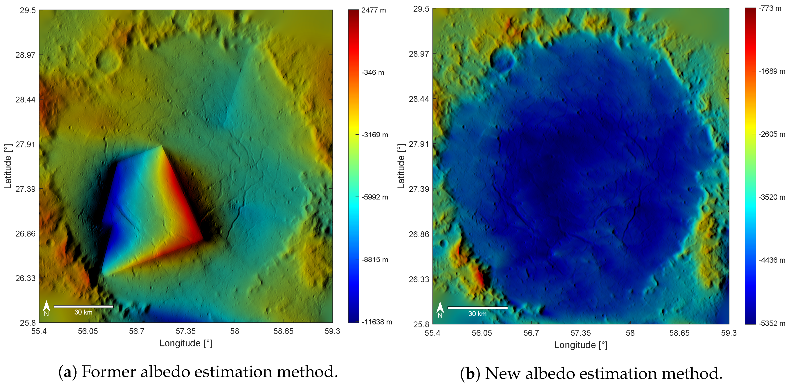
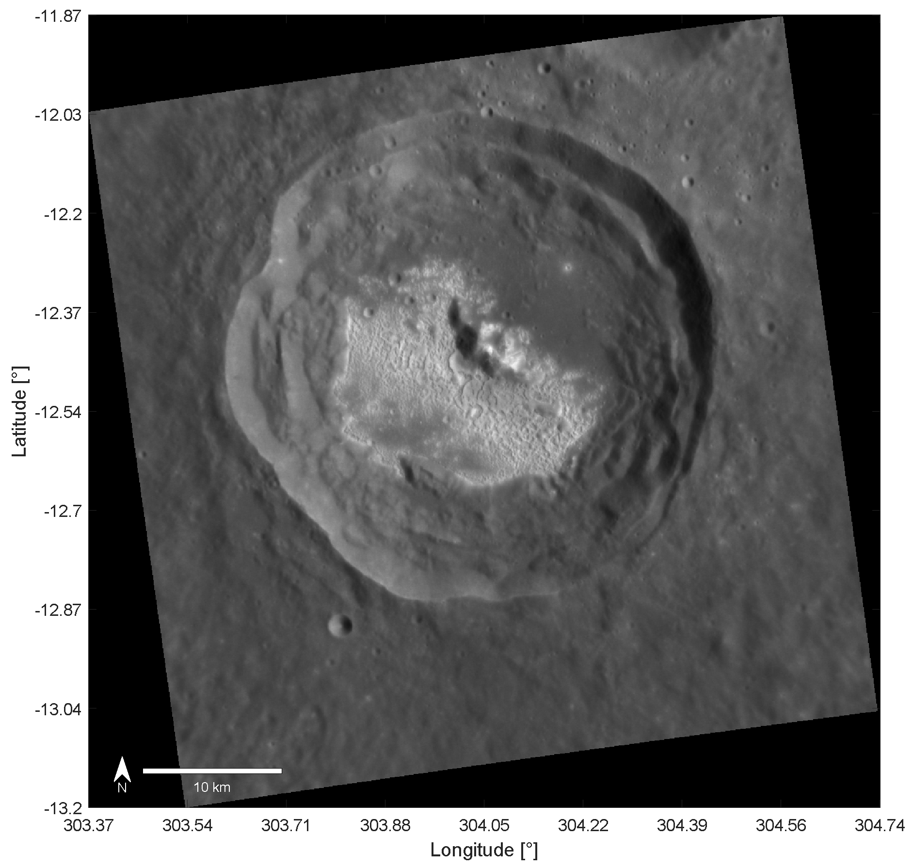
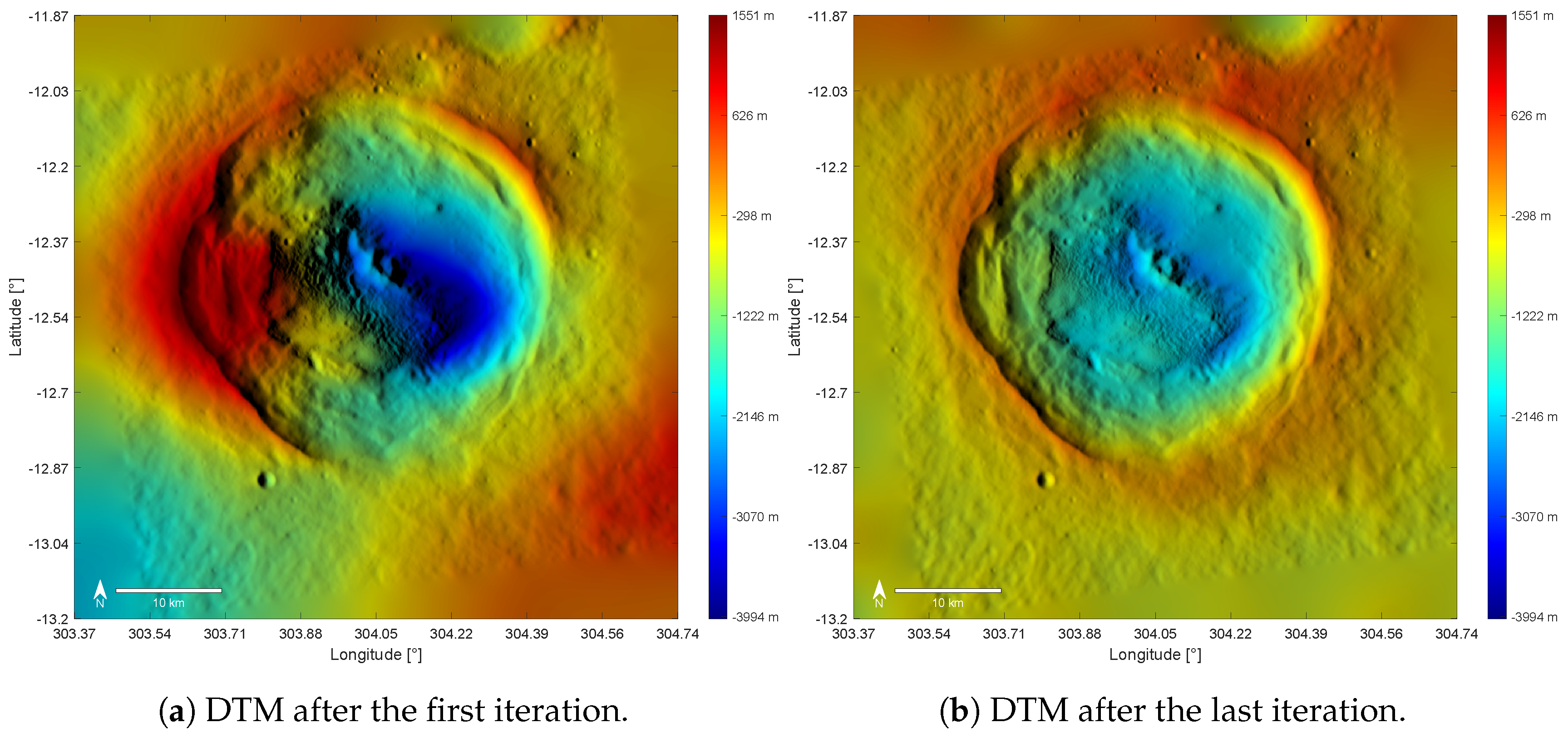
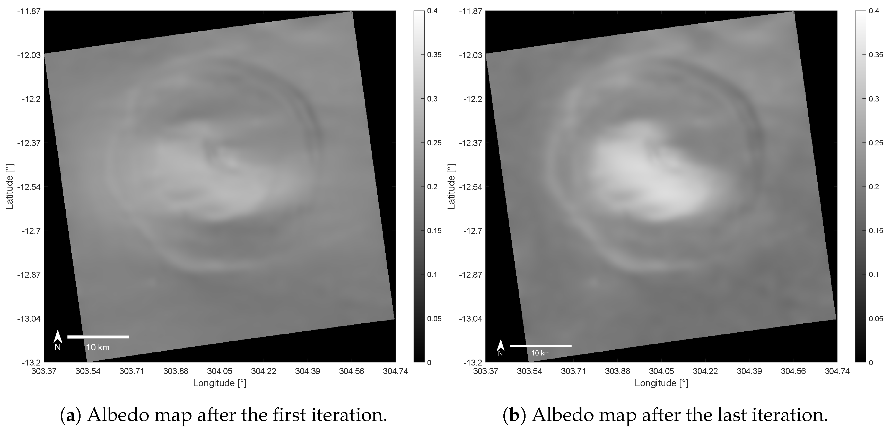
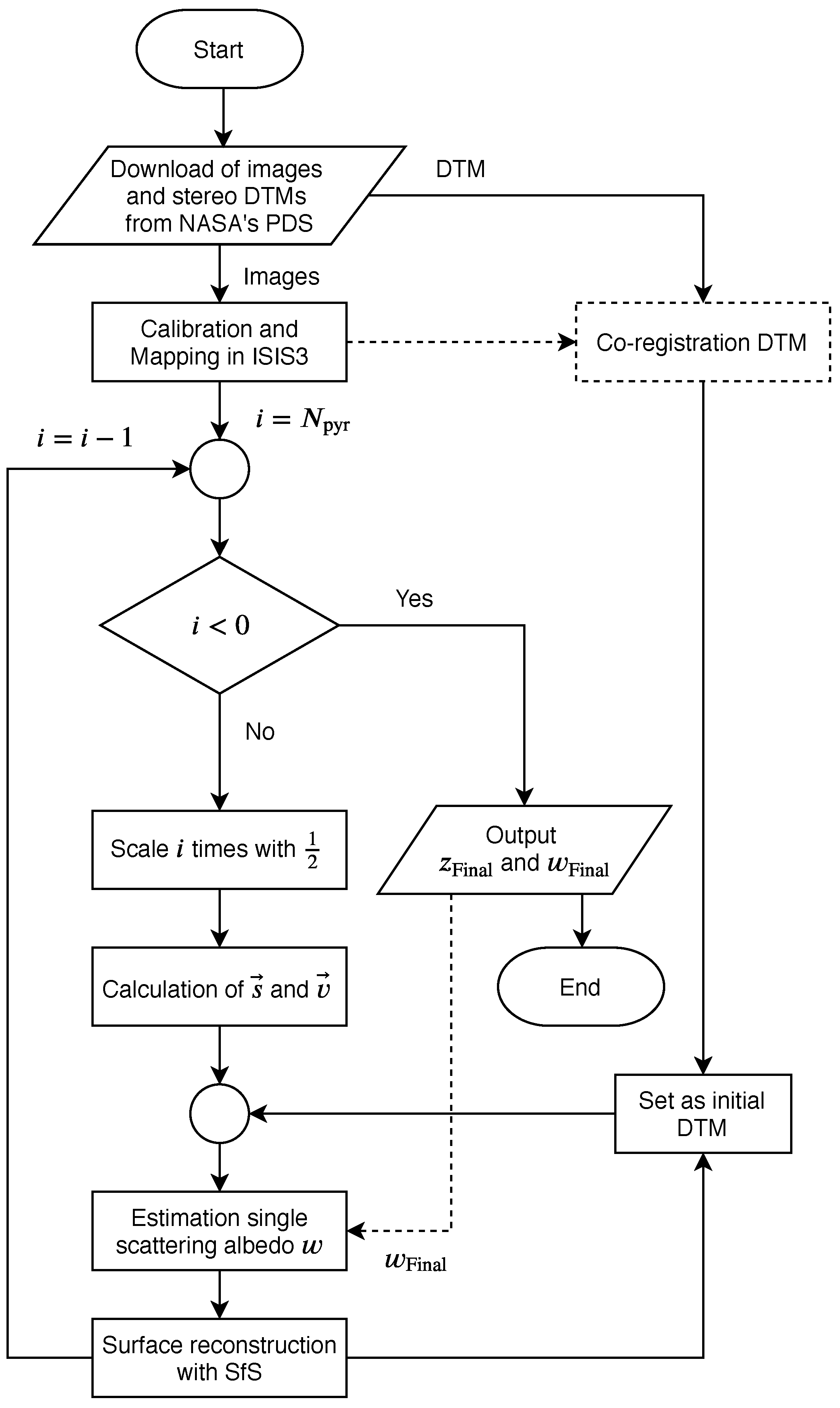
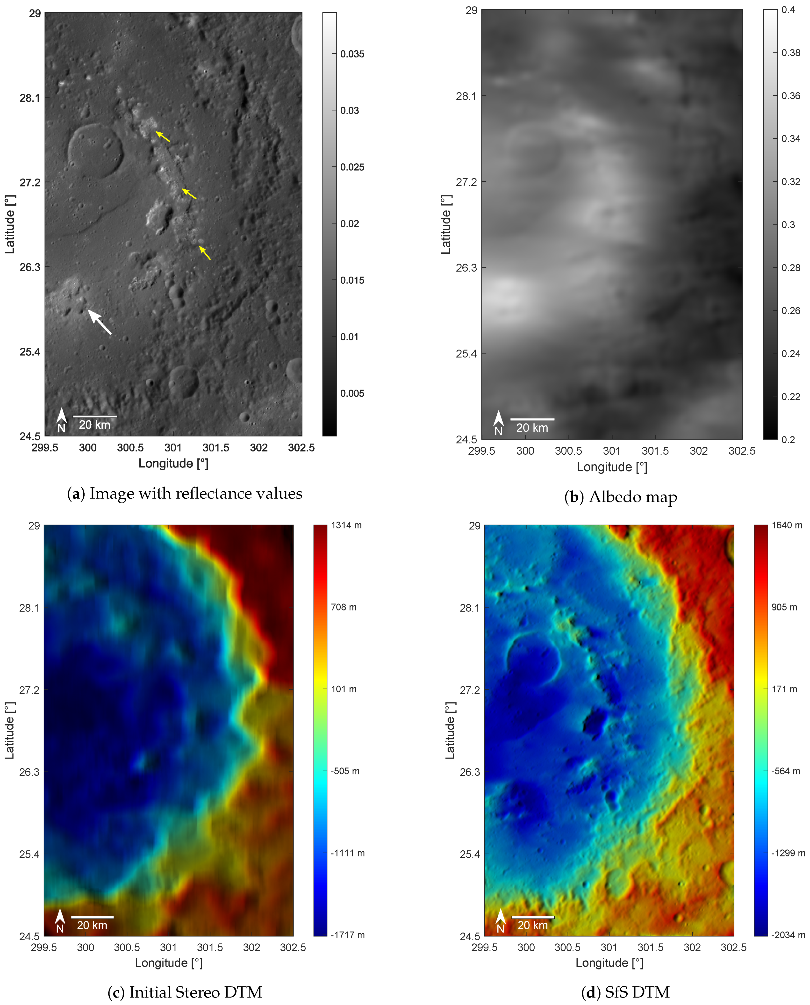
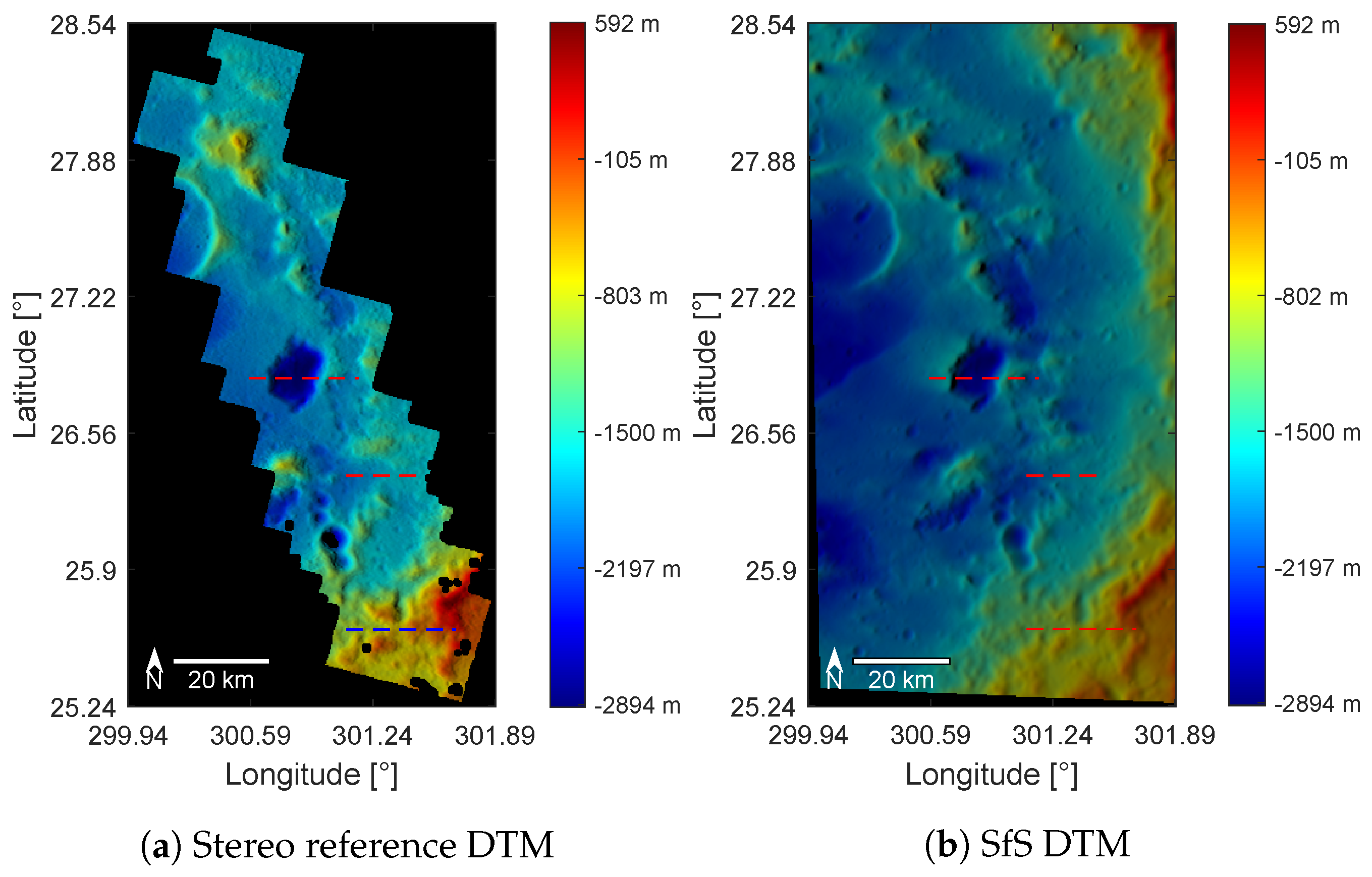
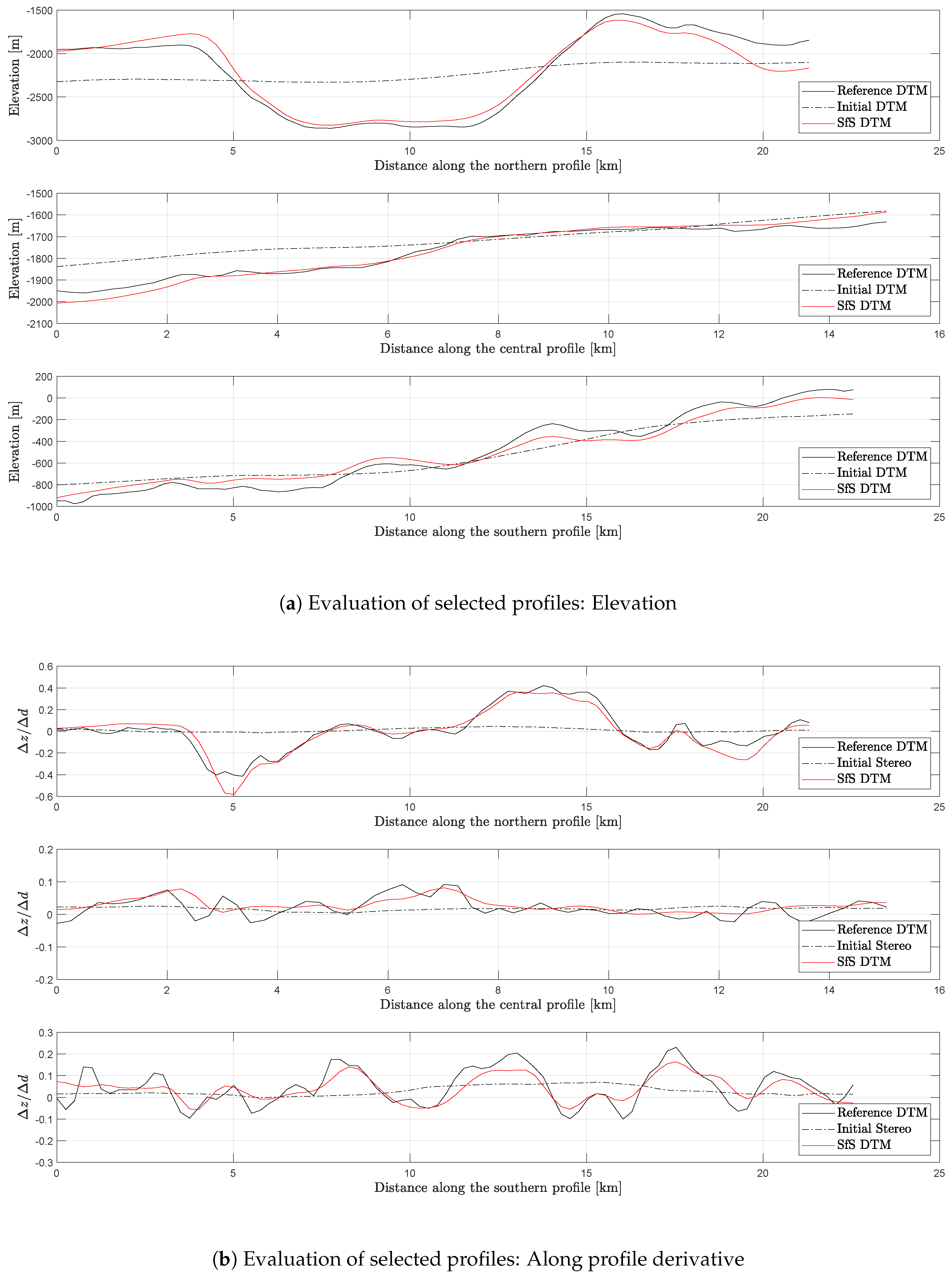
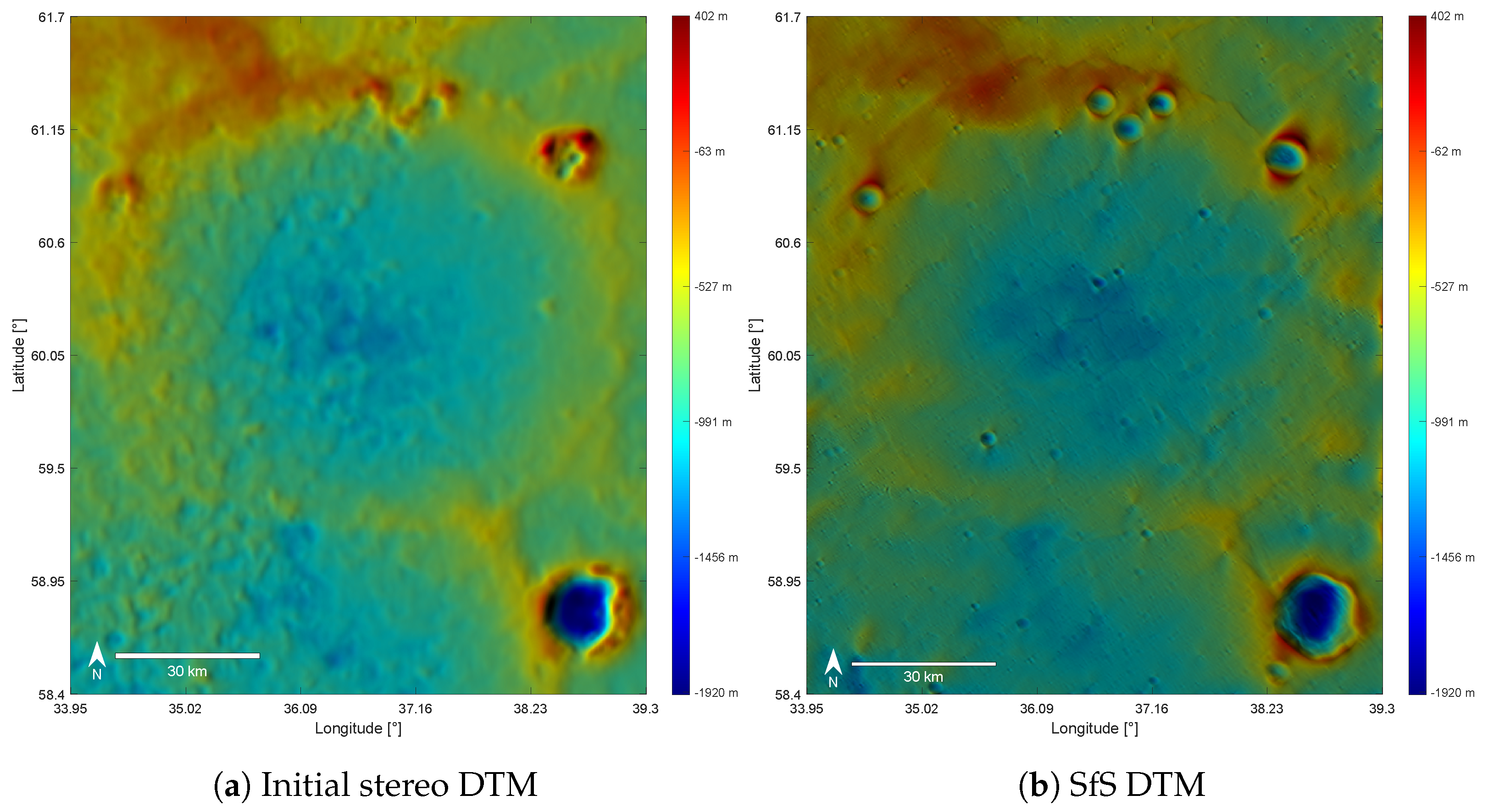
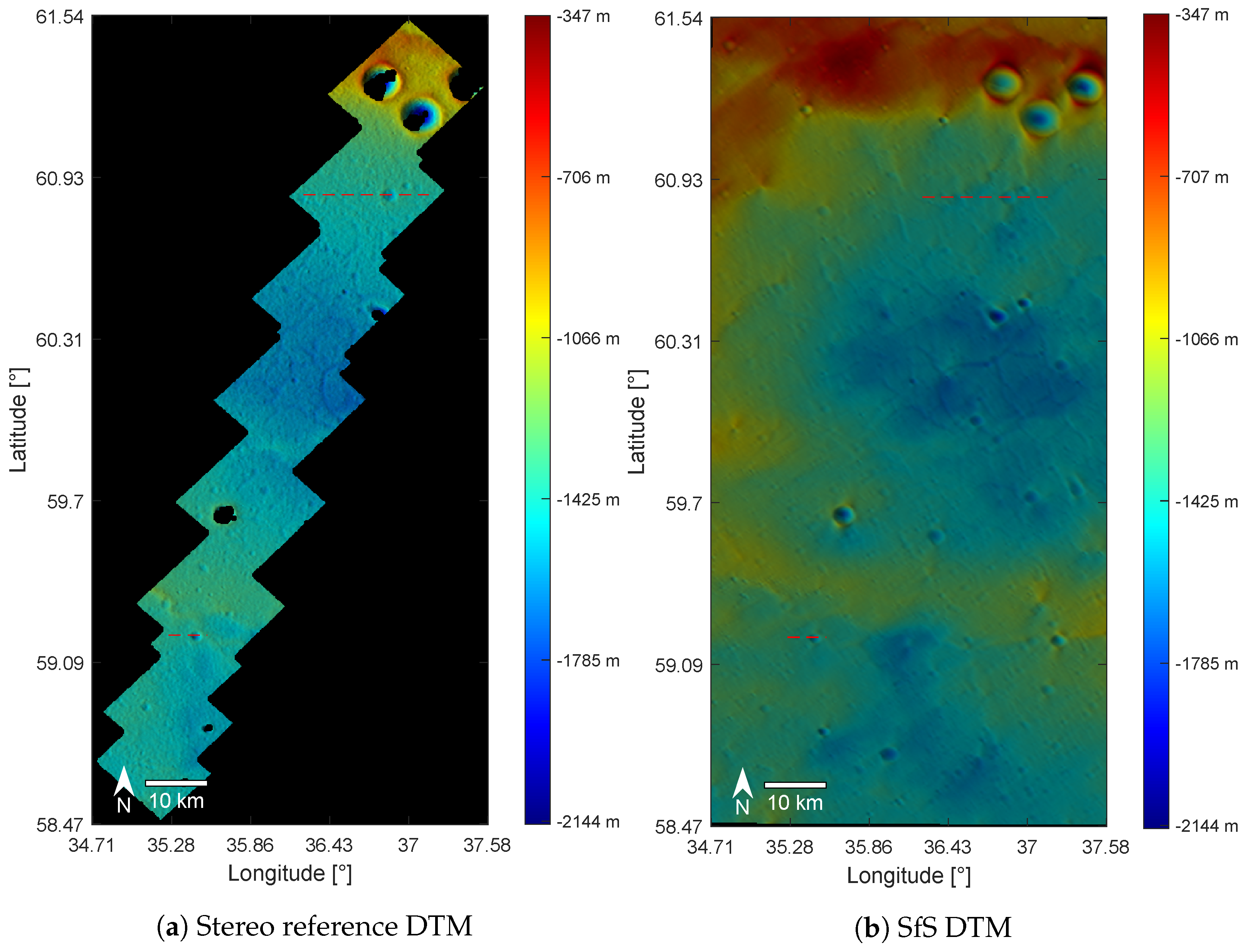
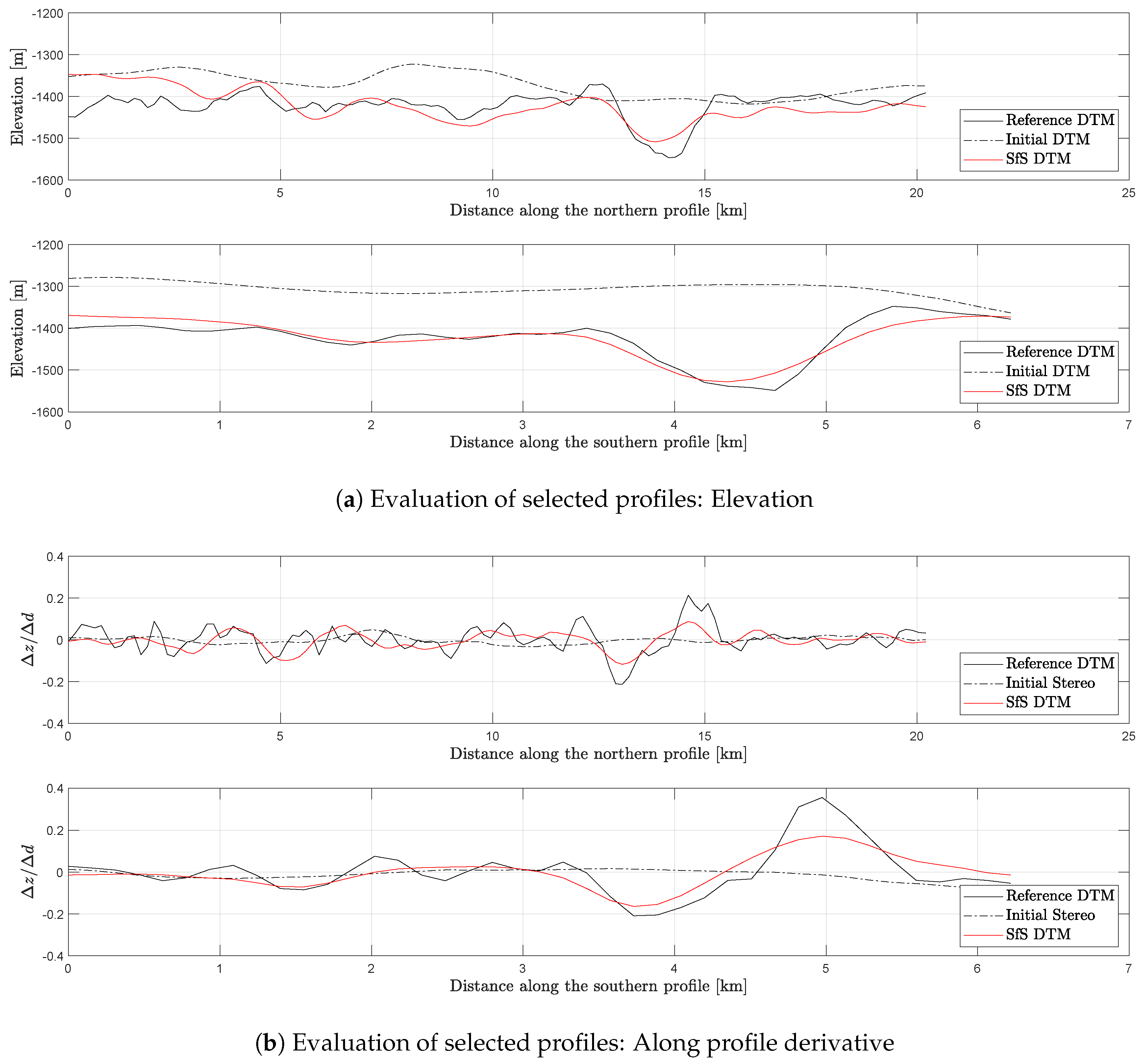
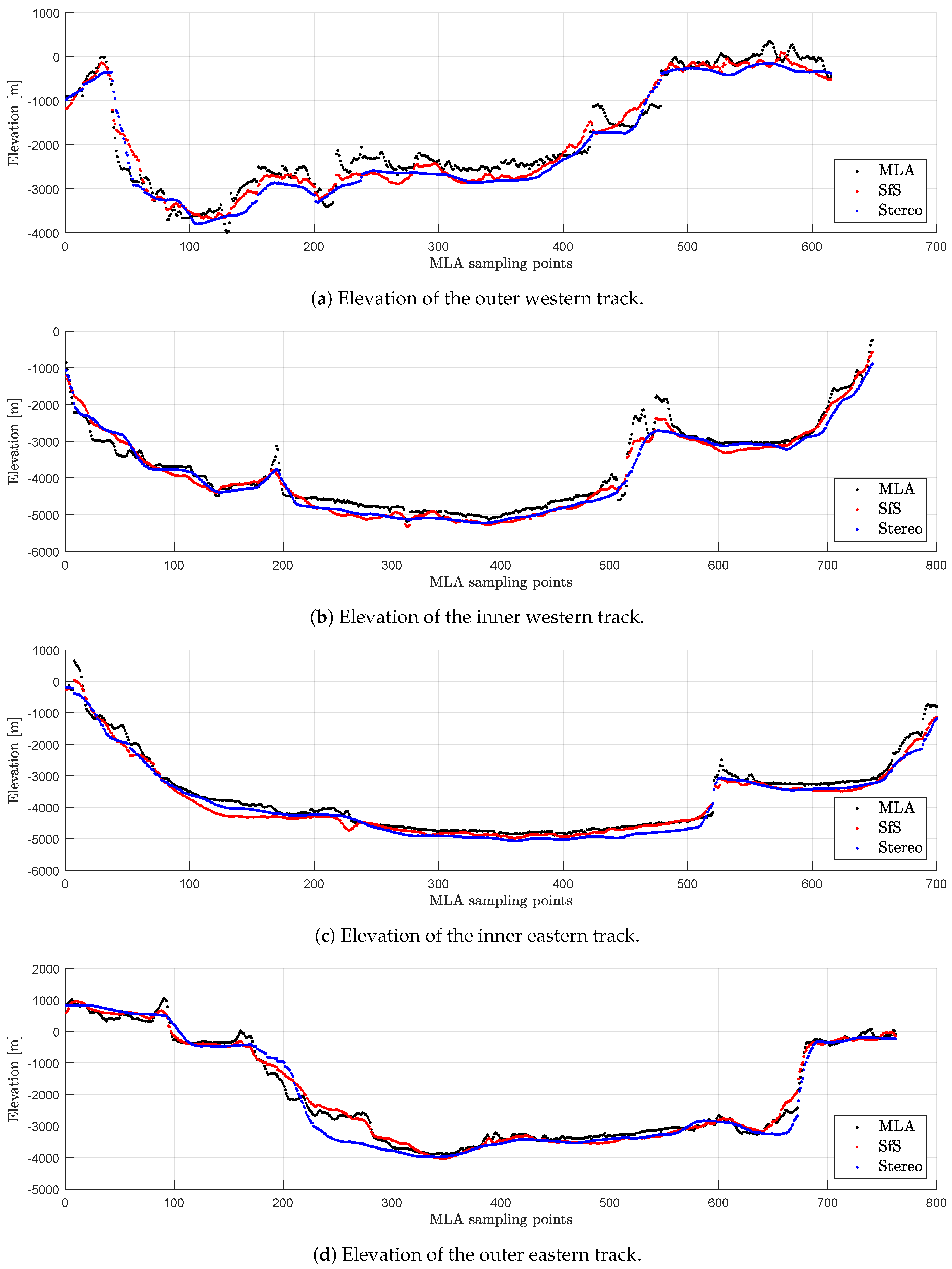
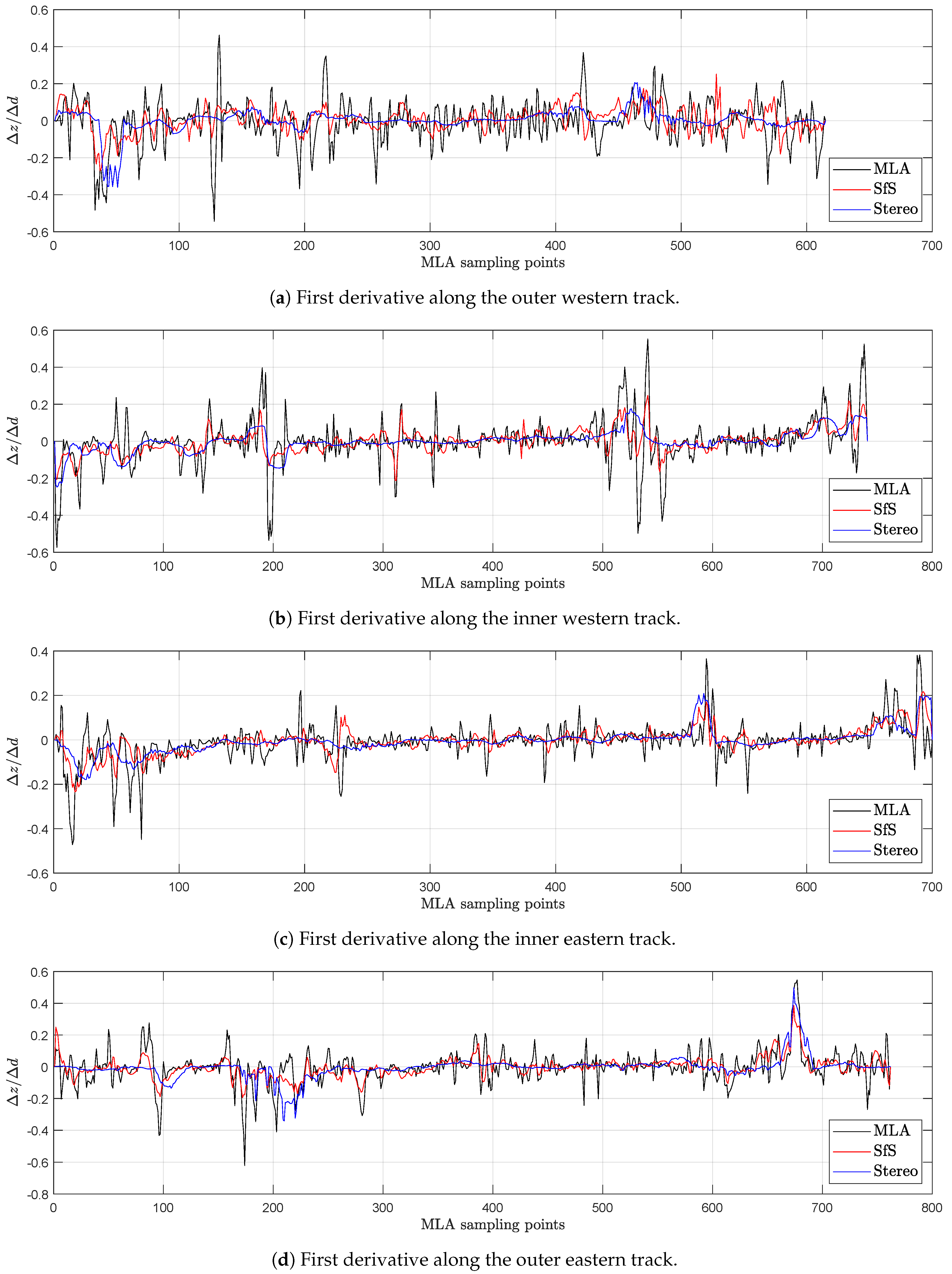
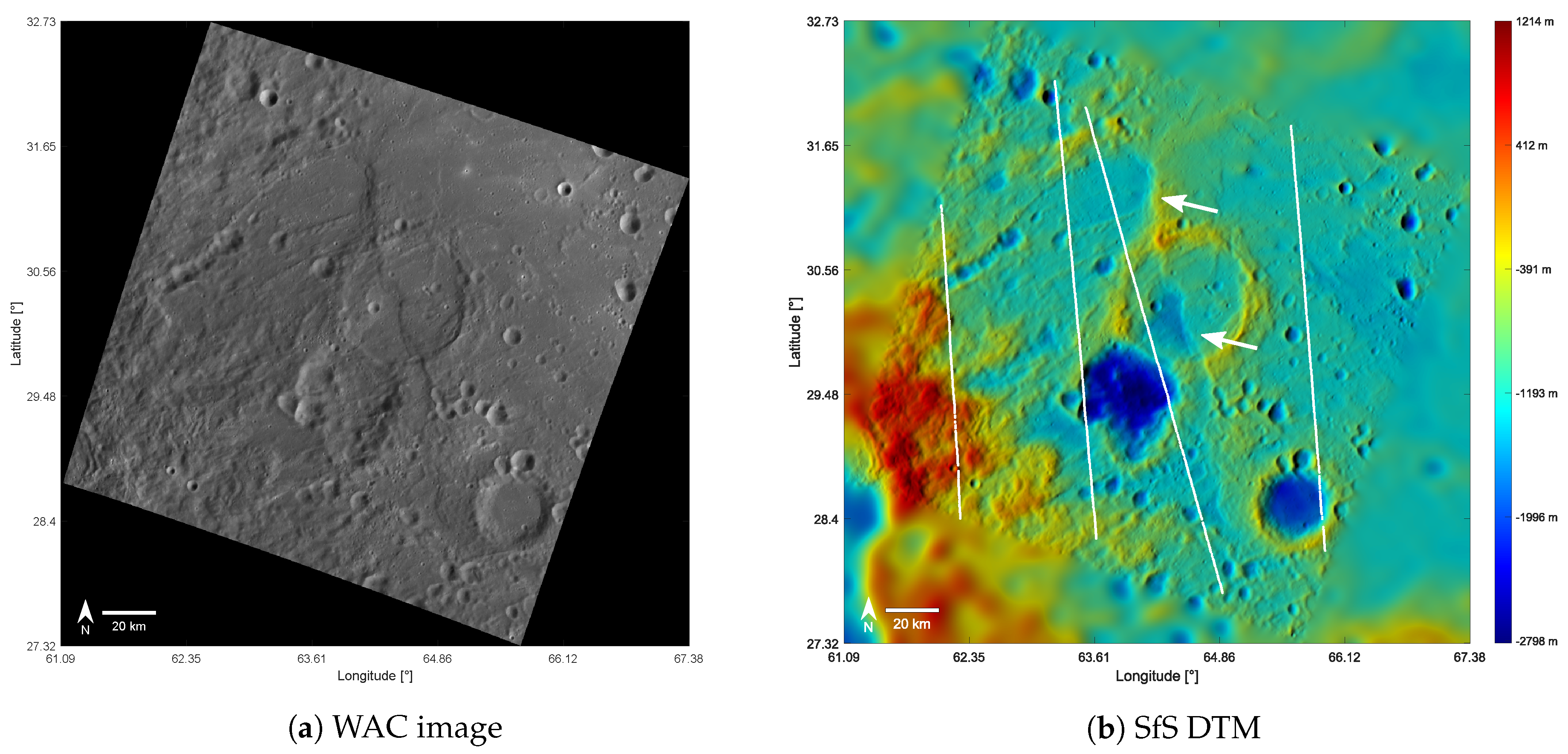
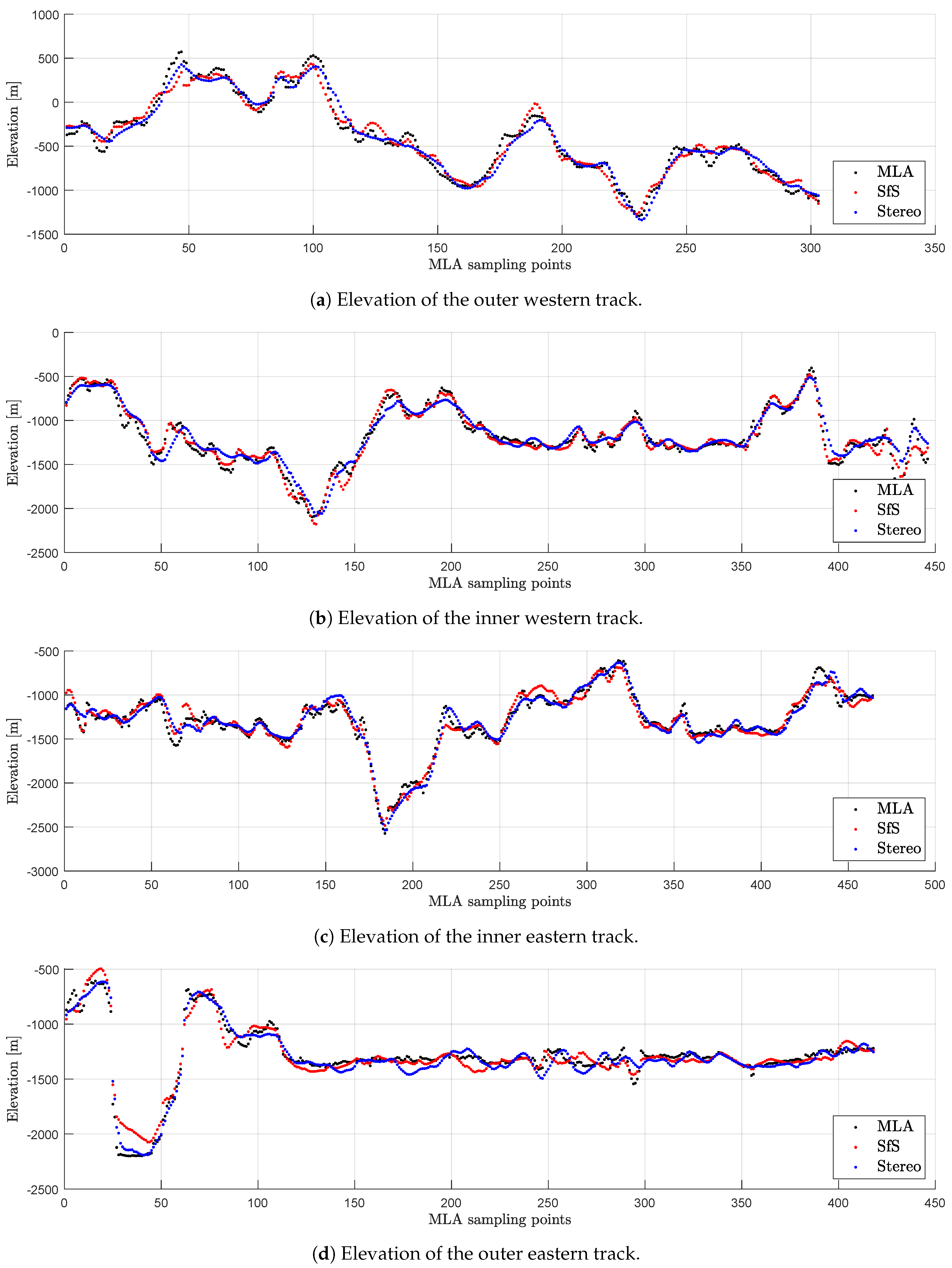
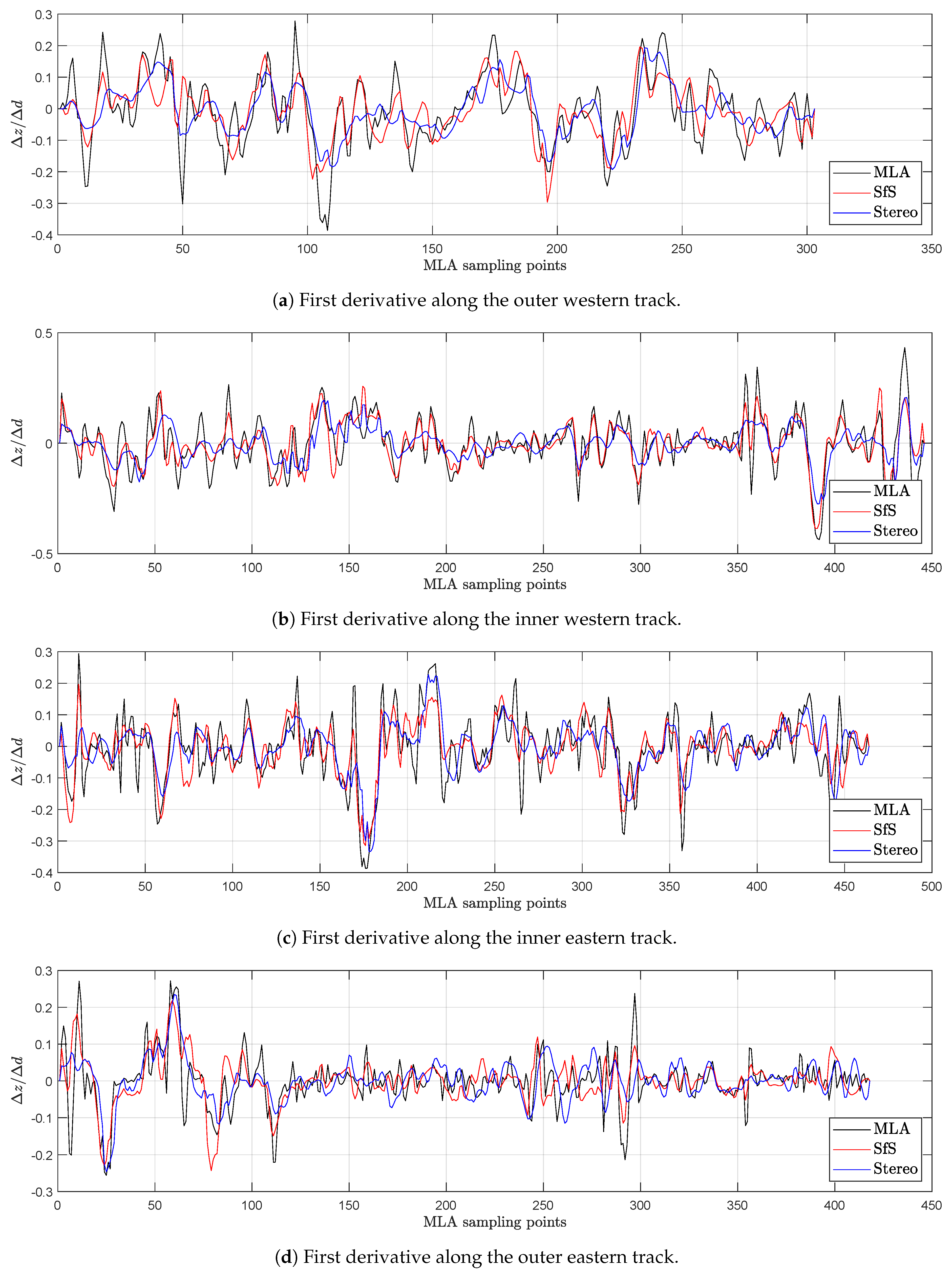
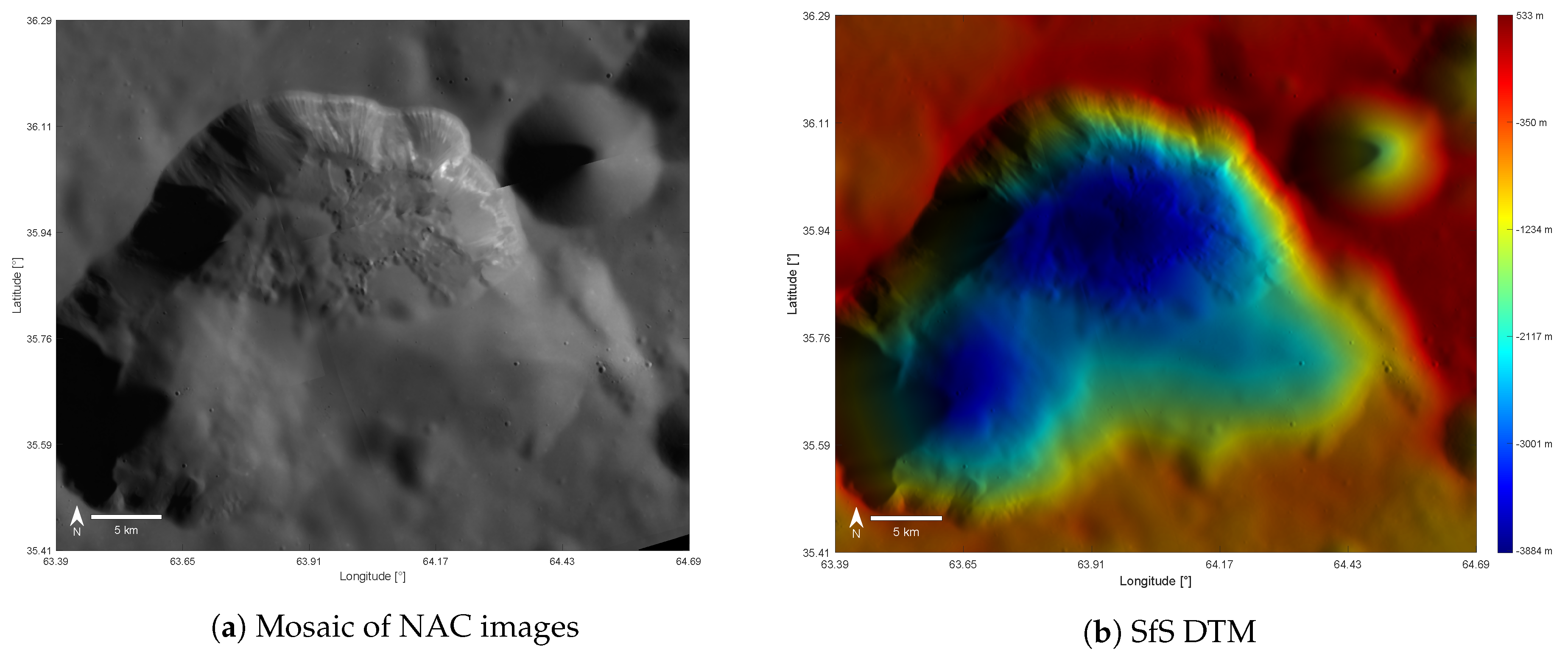
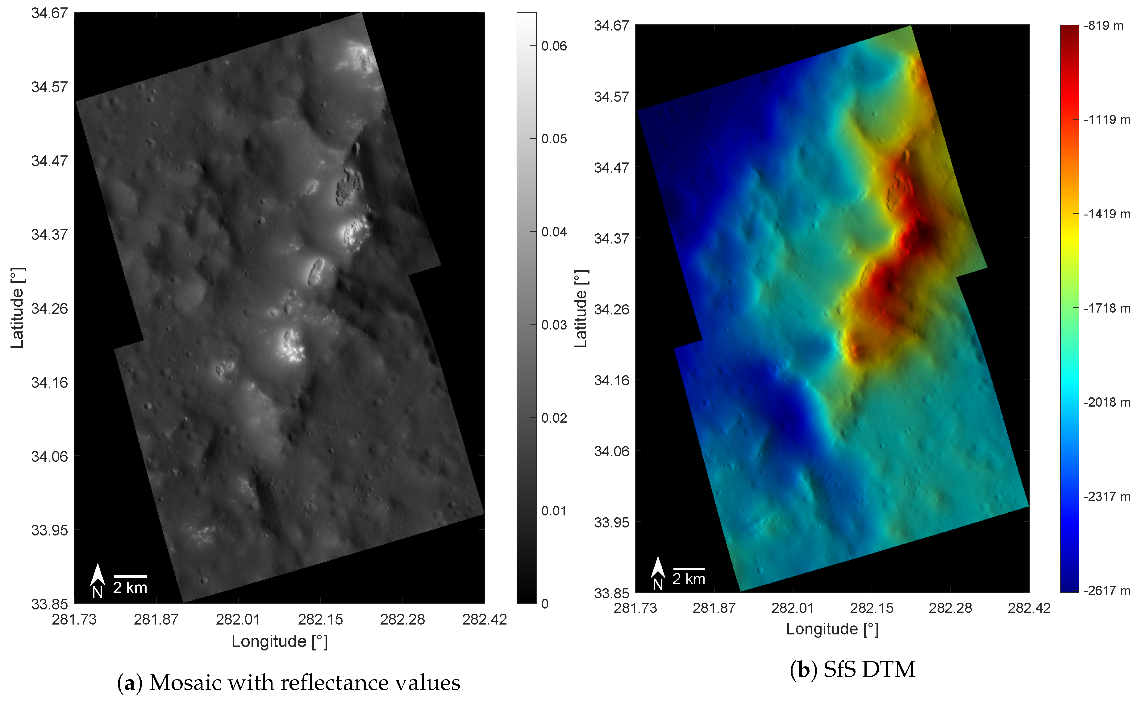
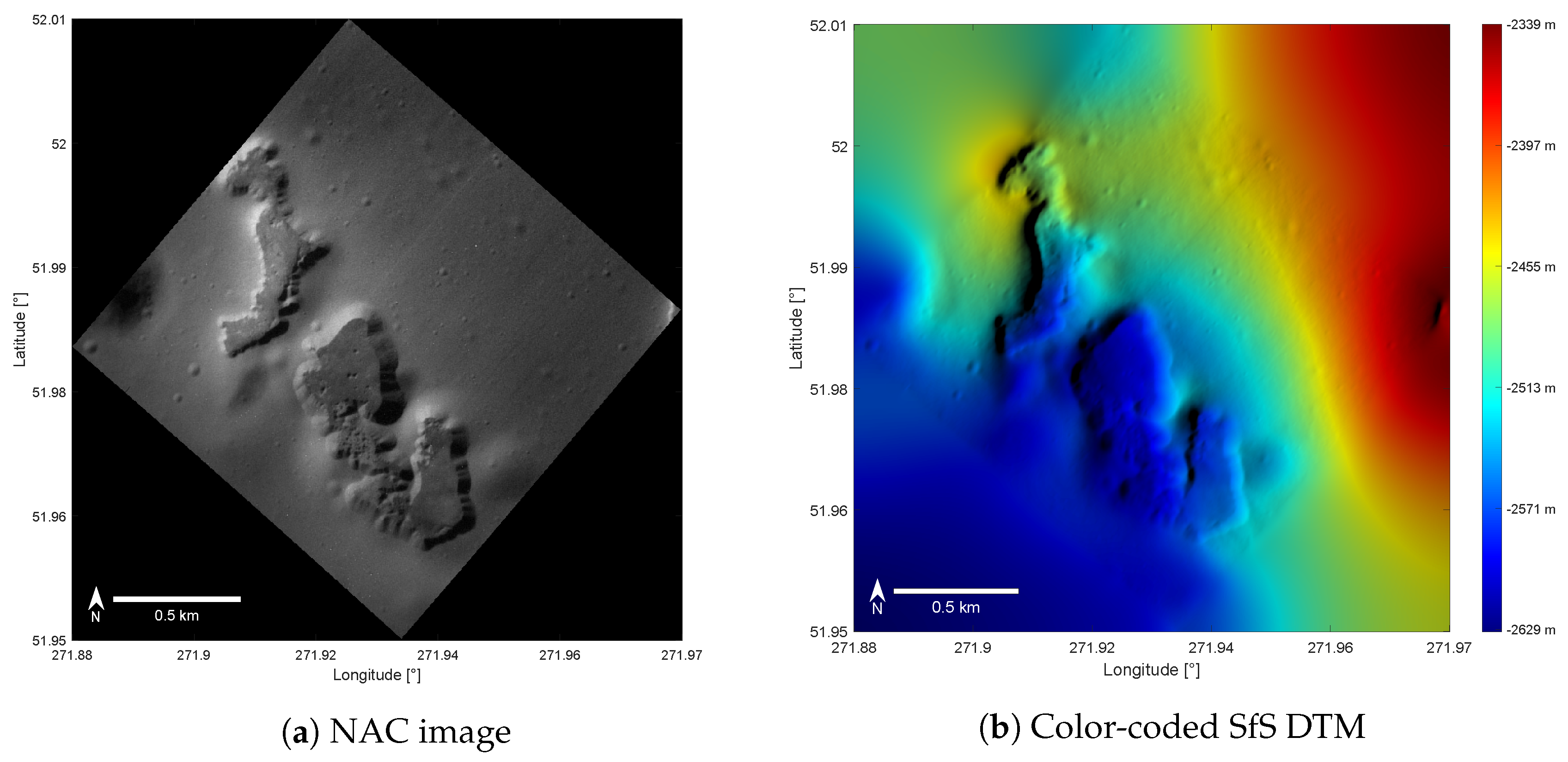
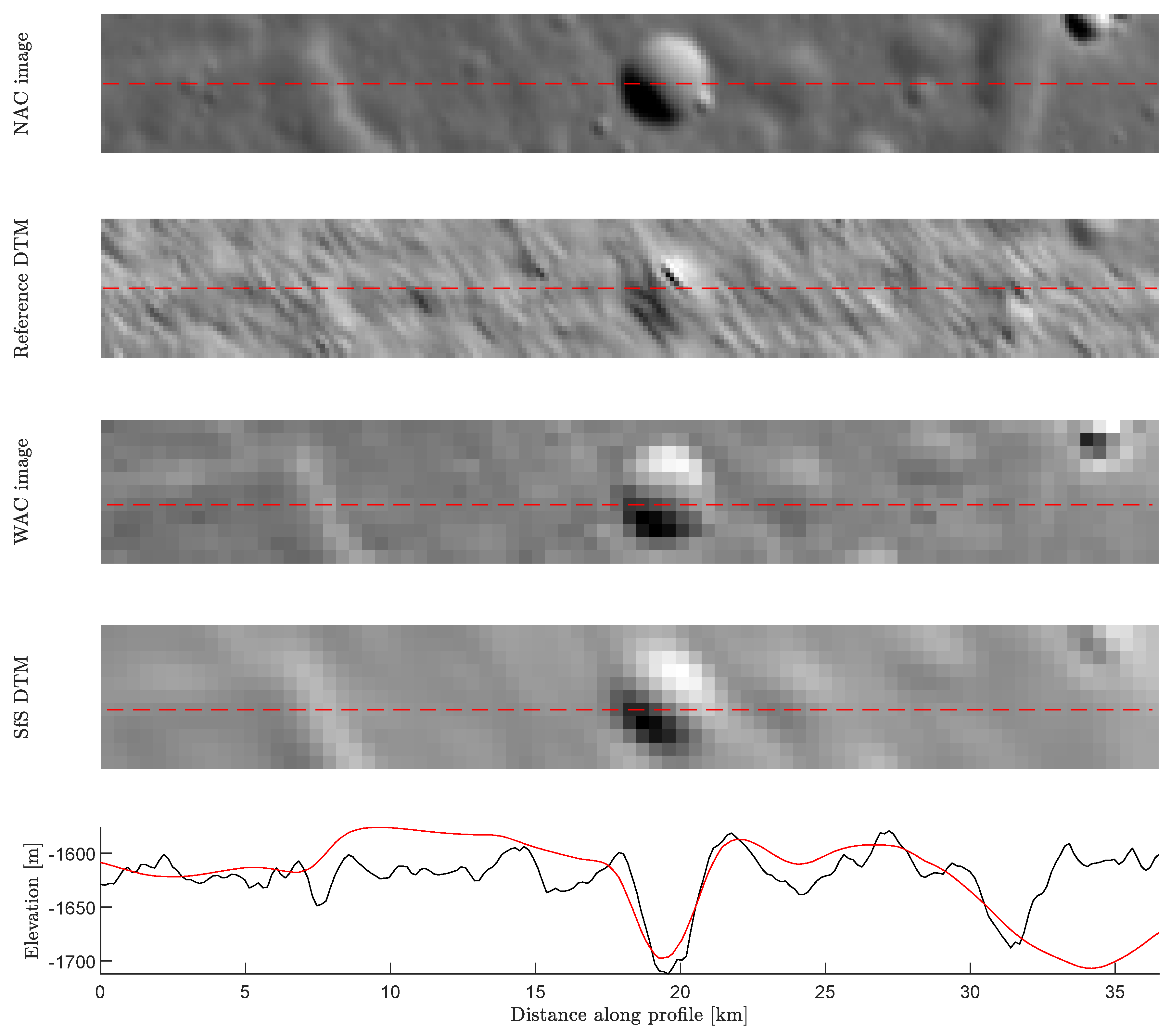
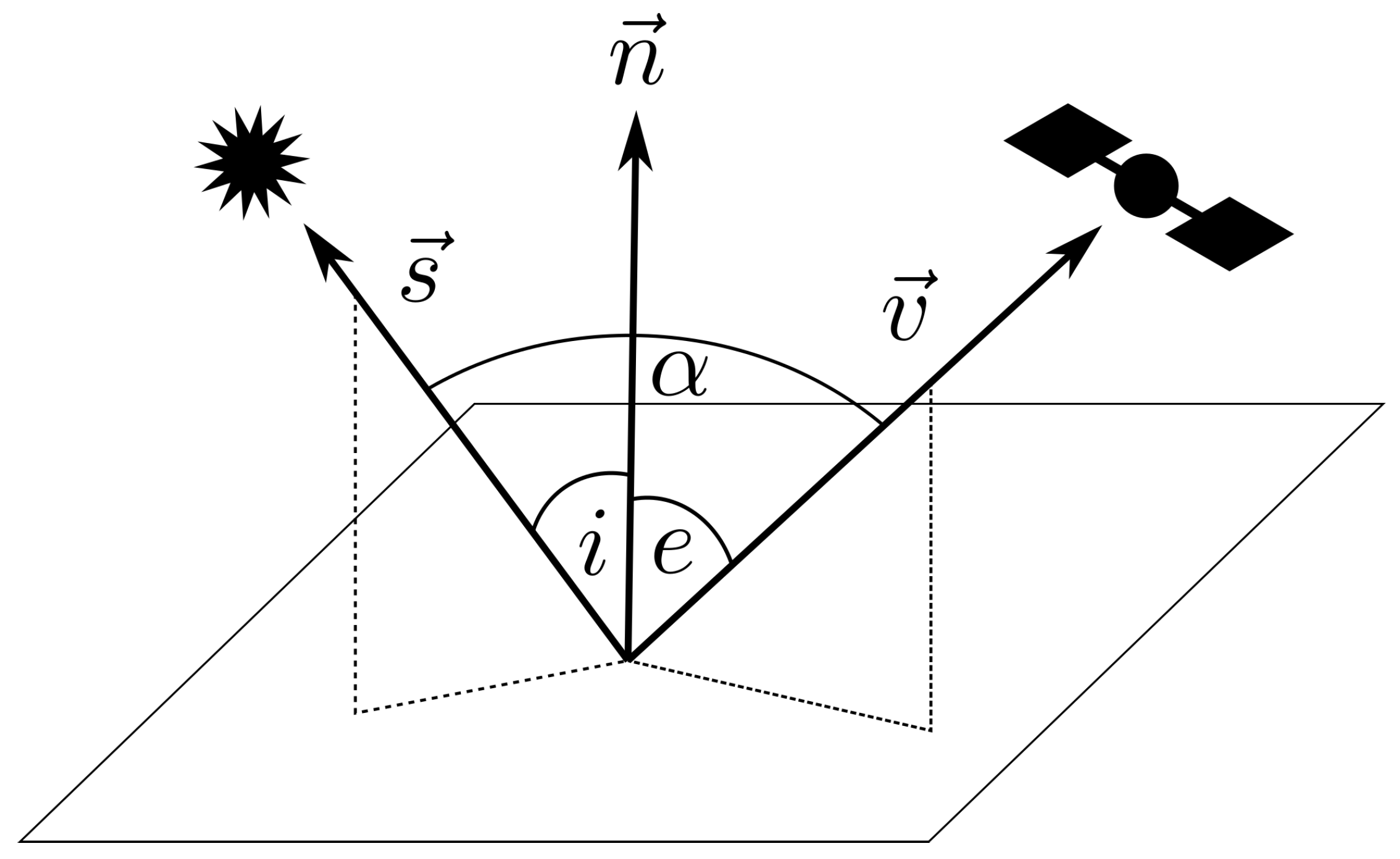
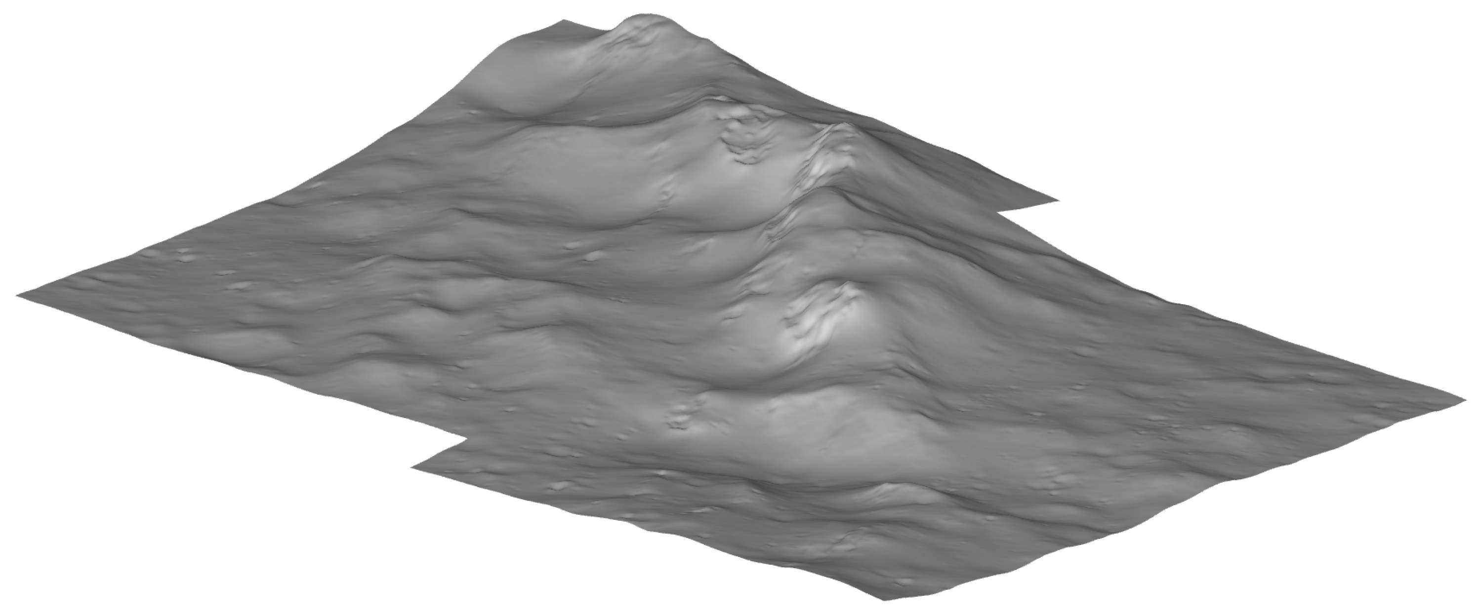
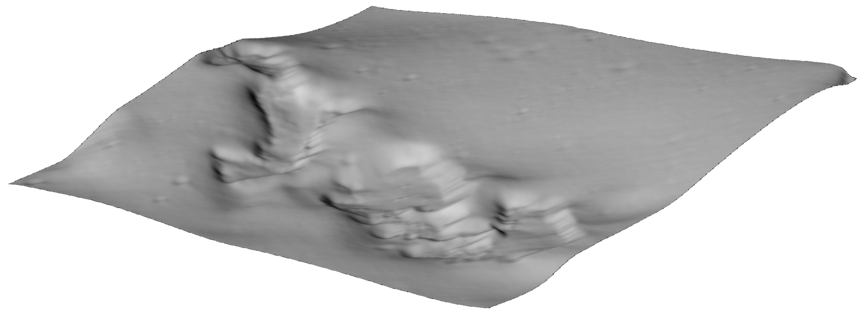
Table 1.
Overview of surface reconstruction on Mercury.
| Publication | Year | Method | Dataset | m/Pixel | Coverage |
|---|---|---|---|---|---|
| Hapke et al. [20] | 1975 | Photoclinometry | Mariner 10 | 20,000 | Profiles |
| Mouginis-Mark and Wilson [21], Mouginis-Mark and Wilson [22] | 1979 | Photoclinometry | Mariner 10 | n.a. | Profiles, topographic maps |
| Watters et al. [23] | 1997 | Stereo, Photoclinometry | Mariner 10 | 500 | Local DTM of Discovery Rupes |
| Zuber et al. [33] | 2012 | Laser Altimetry | MLA | 250 | Northern hemisphere DTM |
| Fassett [29] | 2016 | Stereo | MDIS | >45 | Local DTMs |
| Becker et al. [24] | 2016 | Stereo | MDIS | 665 | Global DTM |
| Preusker et al. [27] | 2018 | Stereo | MDIS | 222 | Quadrangle DTMs |
| This work | 2020 | SfS | MDIS | >3.3 | Local DTMs |
Table 2.
Overview of different SfS approaches.
| Publication | Year | Reflectance Model | Constraint | Albedo Estimation | ||
|---|---|---|---|---|---|---|
| Absolute Depth | Relative Depth | Smooth- Ness | ||||
| Horn [14] | 1990 | Lambert | no | no | yes | no |
| Shao et al. [36] | 1991 | Lambert | yes | no | yes | no |
| Kirk [34], Kirk et al. [42] | 1987 2003 | Minnaert, Lunar- Lambert | no | no | n.a. | no |
| Grumpe and Wöhler [10], Hess et al. [11] | 2014 2019 | Hapke | yes | yes | no | yes |
| Wu et al. [15], Liu and Wu [37] | 2018 2020 | Lunar-Lambert | no | yes | no | yes |
| Alexandrov and Beyer [12] | 2018 | Lunar-Lambert | yes | no | yes | yes |
| Jiang et al. [16], Douté and Jiang [38] | 2019 | Ross-Thick Li-Sparse kernels | yes | no | no | no |
| This work | 2020 | Hapke | yes | yes | no | yes |
Table 3.
Global photometric parameters of Mercury from Warell [44].
Table 3.
Global photometric parameters of Mercury from Warell [44].
| Parameter | Symbol | Value |
|---|---|---|
| DHG parameter | b | |
| c | ||
| SHOE amplitude | ||
| SHOE width | ||
| Mean surface roughness angle |
Table 4.
Properties of the DTMs and original images used for the first evaluation method.
| Property | Praxiteles Crater | Ghost Crater |
|---|---|---|
| Resolution of the image | 250 m/pixel | 155 m/pixel |
| Initial stereo DTM | Global (665 m/pixel) [24] | DLR Quadrangle H05 (220 m/pixel) [27] |
| Stereo reference DTM | 301E27N_0 (65 m/pixel) [29] | 36E60N_0 (55 m/pixel) [29] |
| MAD reference DTM to MLA [29] | ||
| Latitude | 24.5N to 29N | 58.4 N to 61.7N |
| Longitude | 299.5E to 302.5E | 33.95 E to 39.3E |
| Central meridian | 300.98 | 36.18 |
Table 5.
RMSE of elevation and along profile derivative of the SfS profiles to the reference DTM profiles from Figure 9 at a resolution of 250 m/pixel.
Table 5.
RMSE of elevation and along profile derivative of the SfS profiles to the reference DTM profiles from Figure 9 at a resolution of 250 m/pixel.
| Profile | RMSE | |
|---|---|---|
| Elevation [m] | Along Profile Derivative | |
| Northern | 120.00 | 0.061 |
| Central | 24.14 | 0.025 |
| Southern | 69.22 | 0.046 |
Table 6.
RMSE of elevation and along profile derivative of the SfS profiles to the reference DTM profiles from Figure 11 at a resolution of 155 m/pixel.
Table 6.
RMSE of elevation and along profile derivative of the SfS profiles to the reference DTM profiles from Figure 11 at a resolution of 155 m/pixel.
| Profile | RMSE | |
|---|---|---|
| Elevation [m] | Along Profile Derivative | |
| Northern | 34.88 | 0.053 |
| Southern | 20.05 | 0.062 |
Table 7.
RMSE of the elevation (Figure 14) and the first derivative (Figure 15) along the tracks in Figure 13b calculated for the SfS DTM and the initial stereo DTM.
| Track | RMSE Elevation [m] | RMSE along Track Derivative | ||
|---|---|---|---|---|
| SfS | Initial Stereo | SfS | Initial Stereo | |
| Outer west | 269.76 | 318.57 | 0.117 | 0.114 |
| Inner west | 236.81 | 291.35 | 0.092 | 0.111 |
| Inner east | 229.94 | 252.46 | 0.072 | 0.074 |
| Outer east | 172.52 | 305.22 | 0.078 | 0.093 |
Table 8.
RMSE of the elevation (Figure 17) and the first derivative (Figure 18) along the tracks in Figure 16b calculated for the SfS DTM and the initial Stereo DTM.
| Track | RMSE Elevation [m] | RMSE along Track Derivative | ||
|---|---|---|---|---|
| SfS | Initial Stereo | SfS | Initial Stereo | |
| Outer west | 89.82 | 82.73 | 0.077 | 0.077 |
| Inner west | 68.81 | 96.29 | 0.069 | 0.092 |
| Inner east | 77.06 | 74.39 | 0.065 | 0.073 |
| Outer east | 77.00 | 60.00 | 0.056 | 0.060 |
Publisher’s Note: MDPI stays neutral with regard to jurisdictional claims in published maps and institutional affiliations. |
© 2020 by the authors. Licensee MDPI, Basel, Switzerland. This article is an open access article distributed under the terms and conditions of the Creative Commons Attribution (CC BY) license (http://creativecommons.org/licenses/by/4.0/).
Share and Cite
MDPI and ACS Style
Tenthoff, M.; Wohlfarth, K.; Wöhler, C. High Resolution Digital Terrain Models of Mercury. Remote Sens. 2020, 12, 3989. https://0-doi-org.brum.beds.ac.uk/10.3390/rs12233989
AMA Style
Tenthoff M, Wohlfarth K, Wöhler C. High Resolution Digital Terrain Models of Mercury. Remote Sensing. 2020; 12(23):3989. https://0-doi-org.brum.beds.ac.uk/10.3390/rs12233989
Chicago/Turabian StyleTenthoff, Moritz, Kay Wohlfarth, and Christian Wöhler. 2020. "High Resolution Digital Terrain Models of Mercury" Remote Sensing 12, no. 23: 3989. https://0-doi-org.brum.beds.ac.uk/10.3390/rs12233989
Note that from the first issue of 2016, this journal uses article numbers instead of page numbers. See further details here.