Multi-Experiment Observations of Ionospheric Disturbances as Precursory Effects of the Indonesian Ms6.9 Earthquake on August 05, 2018

Abstract

Taking the 2018 Ms6.9 Indonesia earthquake as a case study, the ionospheric perturbations in very low frequency (VLF) transmitters recorded by China Seismo-Electromagnetic Satellite (CSES) were mainly investigated, as well as the multi parameters of the plasma and electromagnetic field. The characteristics of electron density (Ne), GPS TEC, ULF electric field, ion drift velocity, and ionosphere height were extracted and compared with the features of the signal-noise ratio (SNR) from VLF transmitters of NWC at the southern hemisphere and JJI at the northern hemisphere. Most disturbances in VLF radio waves occurred along the orbits near the epicenter within 10 days before the earthquake. Along these orbits, we observed simultaneous modulations in the Ne and ULF electric field, as well as the changed ion drifting directions. There was also high spatial correspondence between both SNR and ionospheric height anomalies over the epicentral and its magnetic conjugate regions. Combined with the multi observations, these results suggest that the genesis of perturbations in signals emitted by VLF transmitters on satellite was more likely related to the overlapped electric field in the preparation area of the earthquake.

1. Introduction

Since last century, a lot of papers have been published concerning the seismic application research using VLF/LF transmitters detected both on ground-based stations and satellites [1,2]. For VLF/LF radio waves, they propagate to long-distance ground-based receivers within the waveguide formed by the lower ionosphere and the Earth [3], and penetrate into the ionosphere or magnetosphere with large attenuation in the lower ionosphere [4]. Ground-based receivers always use antennas to pick up the natural and artificial VLF signals [3,5,6], and satellites detect the VLF/LF signals by an electric field detector and search-coil magnetometer with a wide frequency band [7]. Such transmitters have been illustrated by their sensitivity to the lower ionosphere, their long-term continuous operation time, fixed frequency point with narrow band, and their stable and huge emitted power. Huge and disastrous earthquakes in the world are taken as examples to show the development in VLF waves and seismic research, including Sumatra Mw9.0 earthquake (EQ) in 2004, China Wenchuan Mw7.9 earthquake in 2008, Japan Tohoku Mw9.0 earthquake in 2011, and Nepal Gorkha Mw7.8 earthquake in 2015. Around most strong earthquakes, the ground-based VLF observations were analyzed. For Sumatra earthquake in December 2004, Chakrabarti [8] showed the anomalous sunset terminator shifts, during 22–31 December 2004, of VTX transmitter (17kHz) signal at Kolkata station, and Hayakawa demonstrated an increased fluctuation in the nighttime amplitude, during 21 December 2004 to 2 January 2005, of NWC transmitter signal detected by three Japanese VLF receivers [9], where Horie [10] demonstrated the presence of wave-like structures, with a variable period from 20–30 to about 100 min. In the further investigations about Tohoku earthquake in 2011, Hayakawa reported about a remarkable anomaly in nighttime average amplitude between US NLK transmitter and Japan Chofu receiver on 5–6 March 2011 [11]. However, in the case of Tohoku earthquake in 2011, inconsistent results were discussed. Cohen [12] did not find any anomalous activity in ground-based VLF data, in the days or weeks before EQ, related to four transmitter signals (i.e., JJI, NPM, NWC, and NLK) detected by Onagawa receiver in Japan. However, Ghosh revealed a strong shift in the VLF sunrise terminator signal, a few days before EQ occurrence in Japan in 2011 and also in Nepal in 2015, between JJI transmitter in Japan at 22.2 kHz, and the IERC receiver in India [13]. In addition, Rozhnoi exhibited 8-50-min period disturbances from Hawaiian transmitter after this huge Japanese earthquake, which was possibly related to the internal gravity waves propagation from the excited tsunami region [14]. For the Nepal earthquake, Maurya [15] found the terminator time (TT) shift of 45 min and nighttime fluctuations, one day before EQ, in NWC (19.8kHz, Australia) transmitter signal detected by Allahabad station in Nepal. Furthermore, Phanikumar [16] reported the close relationship between anomalous VLF signals and Mesospheric Ozone content. Besides, satellite data about VLF transmitters was also paid more and more attention in recent years [17]. For Wenchuan Earthquake in 2008 in China, He [18] found one month before the earthquake occurrence, over the epicentral area, a clear decrease of the signal-noise ratio (SNR) associated to five transmitters detected by DEMETER satellite. Additionally, Zhang presented a quick signal drop, occurring a few days before EQ, in the electric field amplitude and SNR from an LF transmitter at 162 kHz in Mongolia and detected by the DEMETER/ICE experiment [19]. All these results show that the VLF transmitter radio wave is an important ionospheric sounding tool and is becoming more and more widely used in the earthquake research community despite the existence of some controversial points due to the complex characteristics of ionospheric precursor generations and wave propagation processes.

Three main parameters have been employed in the VLF radio wave propagation research in relation with seismic activities, which are TT (the meaning of “TT” is stated in the previous paragraph) related to the phase of signals, the average amplitude connected with the strength of signals, and the fluctuations associated with the overlapped ULF waves. To explain these abnormal disturbances occurring before earthquakes, some coupling mechanism and theoretical models have been suggested and developed. The key factor is the ionosphere itself. Hayakawa [20] proceeded to the simulation of a 1.5-km drop in VLF reflection height to explain the anomalies in ground-based VLF signals before Kobe earthquake. Additionally, Rodger and Clilverd [21] employed more realistic propagation models and found that a considerably larger change in the VLF reflection height of about 4 to 11 km could produce the reported effects shown in the TT shift of VLF waves. Chakraborty [22] used the variations in the reflection height and steepness parameter in the Long Wavelength Propagation Capability Program (LWPC) to simulate the propagation process of VLF waves in the waveguide, and showed that the terminator shift towards nighttime only occurred with increased reflection height. The second related factor is about the atmospheric gravity waves (AGWs). Molchanov [22] suggested a complete model about AGW, in which the gas-water release from the seismic region caused atmospheric gravity waves, which penetrated into the ionosphere to modify the ionospheric plasma background and formed a turbulence, in scales of ~1–3 km, where the scattering of VLF waves occurred. Lizunov [23] investigated the amplitude amplification process and the dissipation of AGWs with height and the significant AGW energy transport to modify the plasma parameters of D and E layers, and also wave modification in the neutral atmosphere to form the magneto-hydrodynamic oscillations in the ionosphere and the magnetosphere. Piersanti [24] developed an analytical model of the coupling among the lithosphere, atmosphere, ionosphere, and magnetosphere that was applied just to the 2018 Indonesian EQ based on the acoustic gravity waves (AGW) mechanism.

To confirm the anomalous signals in VLF waves, a network combining transmitter signals and ground reception stations are always intensively considered [9,12], including additional satellite space observations [25]. Besides, other physical parameters have been addressed for further understanding the atmosphere and ionosphere coupling processes. Hence, Zhang [19] found a simultaneous decrease in the LF wave signals and the electron density (Ne) before Wenchuan earthquake using the DEMETER satellite at the topside ionosphere, and pointed to the conflictive relationship of both previous parameters to the wave propagation theory. Phanikumar [16] compared the VLF sub-ionospheric signal and mesospheric ozone before the Nepal earthquakes in 2015, and reported the strong relationship between the pre-seismic VLF signal amplitude/shift in terminator time and mesospheric ozone anomaly in the ionospheric D-layer. Singh and Hobara [26] studied the VLF radio waves and ULF geomagnetic field waveforms around some Japanese earthquakes during 2010–2012, and found that both anomalies occurred simultaneously, within a week before EQs, in most cases.

VLF and ULF investigations have been combined with other physical parameters, like the electron density, the total electron content (TEC), and the electron and ion motions, allowing a better analysis of the coupling processes between earthquake and ionospheric perturbations. Parrot [27] considered magnetic and electric field measurements, and ion and electron densities onboard DEMETER satellite to reveal the ionospheric perturbations around strong earthquakes. Liu [28] firstly combined the technologies at three altitudes to study the plasma variations around the 2005 Sumatra Indonesia Ms7.2 earthquake. They found the enhancement of the plasma density before and after the earthquake using GPS TEC and Ne observations from DEMETER satellite at 710 km, and Ni recorded onboard DMSP satellite at 840 km. Akhoondzadeh [29] used the data from three satellites, i.e., SWARM satellites (A, B, and C), MODIS-Aqua satellite, and ECMWF (European Centre for Medium-Range Weather Forecasts), and found a potential seismic anomalies around the Ecuador Mw7.8 earthquake on 16 April 2016. Such seismic anomalies have been interpreted as an effect of the lithosphere, and then transferred to the atmosphere and ionosphere. It is becoming a promising tool for multi experiments in the LAIC mechanism research.

In this paper, we combine multi physical observational parameters recorded by China Seismo-Electromagnetic Satellite (CSES) weeks before the Indonesia earthquake occurrence, on 5 August 2018. We investigate anomalies recorded in the VLF transmitter signals above the seismic region, and provide further suggestions in the understanding of the relationship between the seismic VLF signals disturbances and the physical processes.

2. Background Information

2.1. CSES Satellite

CSES satellite was successfully launched on 2 February 2018. The main objectives of this mission are to monitor the near-Earth space environment and investigate possible electromagnetic perturbations related to natural disasters and human activities [30]. The satellite has a circular Sun-synchronous orbit at an altitude of about 507 km, an inclination of 97.4°, a descending node at 14:00LT, and a designed lifetime of 5 years. The orbit is strictly revisited each 5 days and all payloads are designed to operate in the region within the latitude of ±65°. Eight scientific payloads have been installed onboard the satellite, including High Precision Magnetometer (HPM), Electric Field Detector (EFD) and Search Coil Magnetometer (SCM) for electromagnetic field detection; Langmuir Probe (LAP) and Plasma Analyzer Package (PAP) for plasma parameters; High Energetic Particle Package (HEPP) and High Energetic Particle Detector (HEPD) together for energetic particles; and GNSS Occultation Receiver (GOR) and Tri-Band Beacon (TBB) for electron density profiles [31]. EFD and SCM cover a wide frequency band, in which EFD are divided into ULF (DC-16 Hz), ELF (6 Hz–2.2 kHz), VLF (1.8–20 kHz), and HF (18 kHz–3.5 MHz). The three frequency bands (i.e., ULF, ELF, and VLF) are also covered by the SCM experiment. The complete electric and magnetic three-component waveforms are stored in ULF and ELF bands, and VLF spectra are computed directly on satellite at SURVEY mode, while VLF waveforms are saved at BURST mode over all the China and the Circum-Pacific and Eurasia seismic belts. To reduce the effects of residual magnetism from the satellite platform, 6 booms are separately extended outside at different directions with a length of 5 m, where 4 are connected to the EFD sensor balls, one to the HPM experiment, and one to the SCM instrument. Zhang [32,33] have described in details the position of the four booms related to electric field experiment, where Ball-a is almost along the −Y direction, Ball-b with 45° to −X and −Z, Ball-c with 45° to +X and −Z, and Ball-d with 30° to +Y and 60° to +Z (X, Y, Z is in satellite coordinate with +X to the satellite flight direction, +Z to the Earth, and +Y being the right-handed crossing direction of Z to X). On the satellite, three spectral components, at three directions between two balls of a-b, c-d, and a-d, are calculated and averaged each 2.048 s in SURVEY mode. On ground data center, the same satellite coordinate system and same three directions of Eab, Ecd, and Ead are used for spectra transform from waveforms at BURST mode.

2.2. VLF Transmitters around Indonesia

There are several VLF transmitters set up on the ground for the purpose of communication and navigation.

Table 1. VLF transmitters around Indonesia.

Code	Country	Frequency(kHz)	Longitude(°E)	Latitude(°N)	Power(kW)
NWC	Australia	19.8	114.20	−21.80	1000
JJI	Japan	22.2	130.81	32.04	200
3SB	China	20.6	103.33	39.60	-
3SA	China	20.6	111.67	25.03	-

indicates the code name, the frequency, the geographical coordinates, and the power of transmitters around Indonesia, i.e., NWC in Australia, JJI in Japan, 3SA and 3SB in China. NWC is the most powerful transmitter in the world with high emitted power of 1000 kW, which ensures that it can penetrate into the ionosphere with large amplitude. Both Chinese transmitters at 20.6 kHz appear to alternate between the two locations; therefore, we will select one of them according to the actual records on CSES, or none of them due to the discontinuity. The effective frequency of the VLF electric field on CSES is 1.8–20 kHz. However, the sampling rate of the EFD/CSES experiment is 50 kHz in the VLF band, which leads to the detection of the signals over 20 kHz. On the basis of the frequency response function in this band, the signals above 20 kHz will be attenuated to a certain extent.

3. Earthquake Study on VLF Transmitters from CSES

An earthquake occurred in Indonesia (Lat.: 8.26°S, Long.: 116.44°E) on 5 August 2018, at 11:46 UT with a magnitude of Ms6.9 and a depth of 34 km. At this time, the CSES satellite had been in operation for 6 months, and most payloads work in a stable status. Aiming at this case, the VLF EFD data were firstly collected from 15 July to 10 August, in 2018. In the data processing, spectra with FFT are derived from BURST mode waveforms and combined with other observations recorded in SURVEY mode for a given full orbit. To reduce the noise background and ensure the consistency of spectra data, we averaged BURST mode observations with a small time interval (i.e., 0.082 s) as that (i.e., 2.048 s) in SURVEY mode. The SNR is calculated using the following equation: $SNR=\frac{2A\left(f_0\right)}{A\left(f_{+}\right)+A\left(f_{-}\right)}$, where f₀ is the recorded transmitter frequency, and f₊ and f_- are the referred frequency as ±200–500 Hz [17,19]. Hereafter, we will use one spectral component of the electric field (Eab, or Ecd or Ead) taking into consideration the quiet space environment.

Figure 1 shows EFD measurements recorded when 2 CSES orbits crossed the epicenter region. The three panels, from the top to the bottom, correspond respectively to the dynamic spectra, the variation of the signal at 20.5 kHz versus the geographical latitudes, and the frequency variation in the bandwidth 15–25 kHz at a geographical latitude of 8.2°S. At both the west and east sides of the epicenter, 4 transmitters with different frequencies can be found. Figure 1 displays powerful and clear emissions at 19.8 kHz from NWC (Australia) and 22.2 kHz from JJI (Japan), and two transmitters frequencies at about 20.5 kHz. Along the #2516-1 orbit on 17 July 2018, the transmitted mode with a stable time interval of [power on] and [power off] is displayed in Figure 1 (second left-panel) at a frequency of 20.5 kHz in the latitude range from −40°S to 0° along the orbit. Along the orbit #2546-1 on 19 July 2018 at the east side of the epicenter, the spectral features are similar with those of #2516-1, but higher strength values at 19.8 and 22.2 kHz are detected at the latitude of −8.2°S. Along this orbit, the power spectrum density in Ead is plotted at 20.4 kHz frequency at the latitude range between −40°S and 40°N, in which two maxima occur at latitudes of −32°S in the southern hemisphere and 26°N in the northern hemisphere, and much higher at the southern hemisphere. Table 1 lists the two transmitters (i.e., 3SB and 3SA) from China emitting at a frequency of 20.6 kHz, which are not detected in spectra (see the first panels of Figure 1) and not the same with those observed here at 20.5 or 20.4 kHz. The sources of the transmitters with frequencies of 20.4 and 20.5 kHz are more likely located at latitudes ~−30°S–32°S in the southern hemisphere. Due to the difficulty to exactly localize both transmitters (i.e., 20.4 and 20.5 kHz), we will not consider those VLF signals in our investigation. On the basis of this analysis, two transmitters will be used in this paper due to their clear locations and their continual emitted modes (i.e., 22.2 and 19.8 kHz).

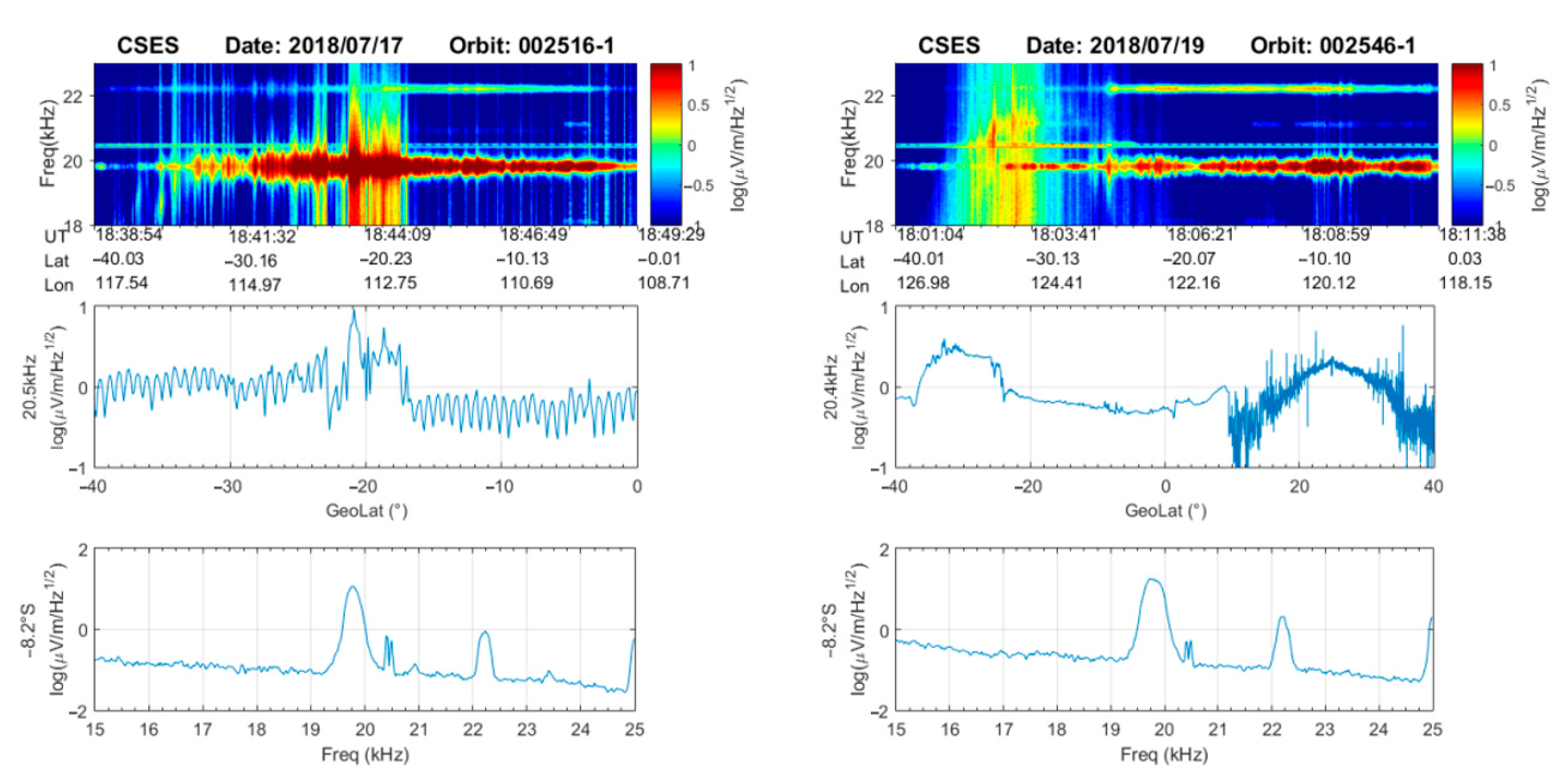
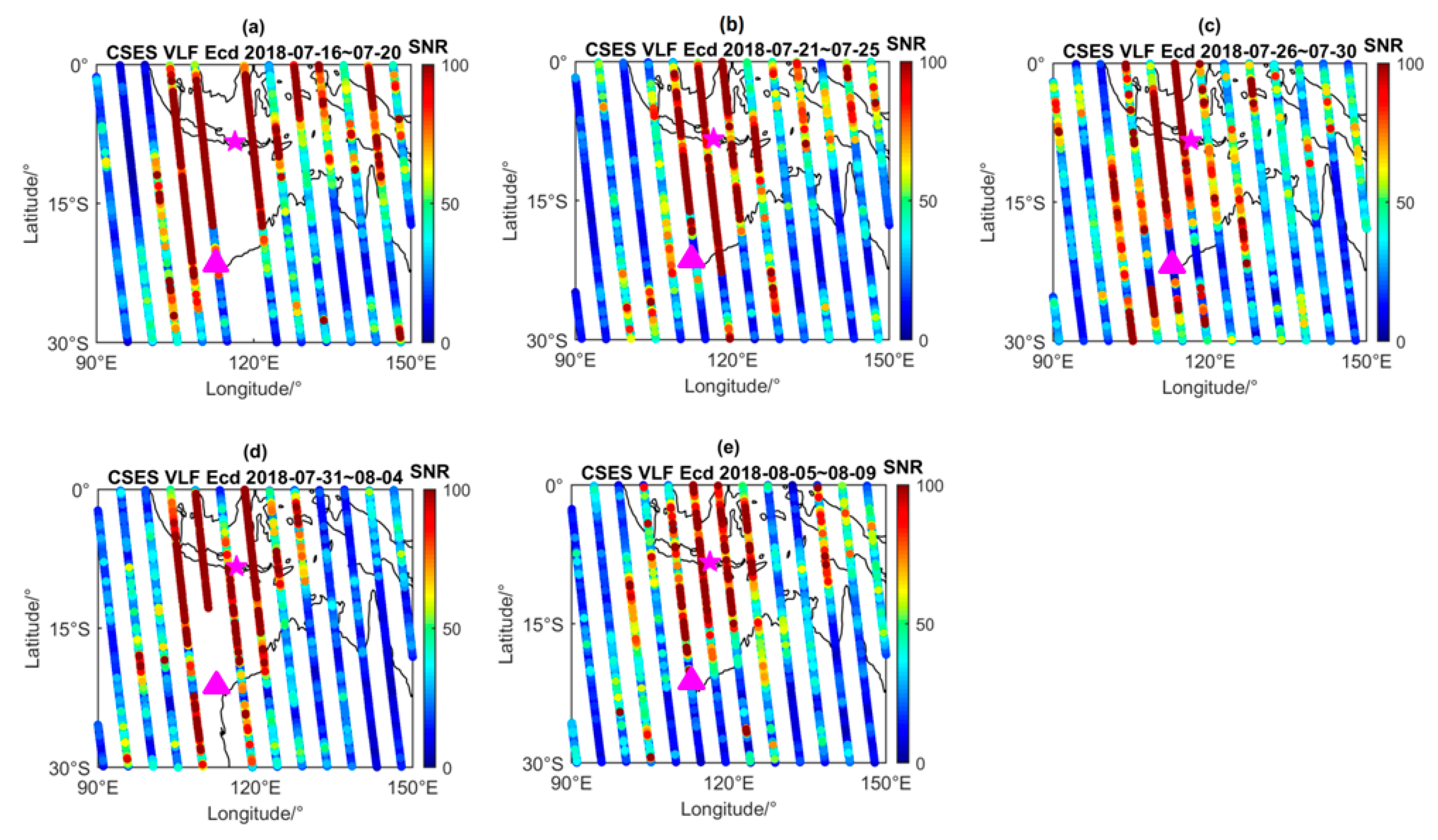
3.1. SNR Analysis from NWC at 19.8 kHz

NWC is one of the most powerful transmitters in the world, and many papers have studied the radio wave signals detected by ground-based stations and satellites due to its strong emitted power, and long-term and stable operation mode. One of the spectral components is selected to do the analysis. From Figure 1, NWC emits the radio waves at 19.8 kHz with a quite wide frequency band, so ~±500 Hz is selected as the preferred background to calculate corresponding SNR values. Figure 2 shows the spatial distribution of SNR from the NWC transmitter from 16 July to 4 August, each 5 days, according to the revisited period of the CSES satellite. It can be seen that the epicenter is located in the covering area of NWC in the southern hemisphere (Table 1, Figure 1), and large values of more than 100 of SNR occurred at all directions around the epicenter during 16 to 25 July (Figure 2a,b). The maximum value of SNR is not located just over the NWC transmitter but inclines to the equator due to the effects from geomagnetic field in the radio wave propagation. Here, we give 5 pictures in 20 days before and 5 days after the earthquake, so each orbit near the epicenter can be compared with its neighboring one, and also its revisited orbits in each panel at the same geographical position. Since 26 July, as shown in Figure 2c, the SNR decreased quickly at the southern and eastern sides of the epicenter with SNR smaller than 70, and 1–5 days before the earthquake (Figure 2d), SNR reduced at the north part along the closest orbit, just at the west side of the epicenter. From 5 to 9 August after the earthquake, the SNR recovered gradually to the normal level in all directions. Within 10 days prior to the earthquake, the perturbations in the NWC transmitter signal were clearly detected by the CSES satellite mainly along three orbits. Only nighttime observations were used in the analysis, and all the studied time periods were in July and August, within the same season. In addition, NWC has less seasonal variation at the topside ionosphere according to DEMETER observations [34]. Therefore, these perturbations in NWC on CSES are not due to seasonal effect but are linked to some internal or external signals in the ionosphere leading to the decrease of NWC transmitter signals on the satellite.

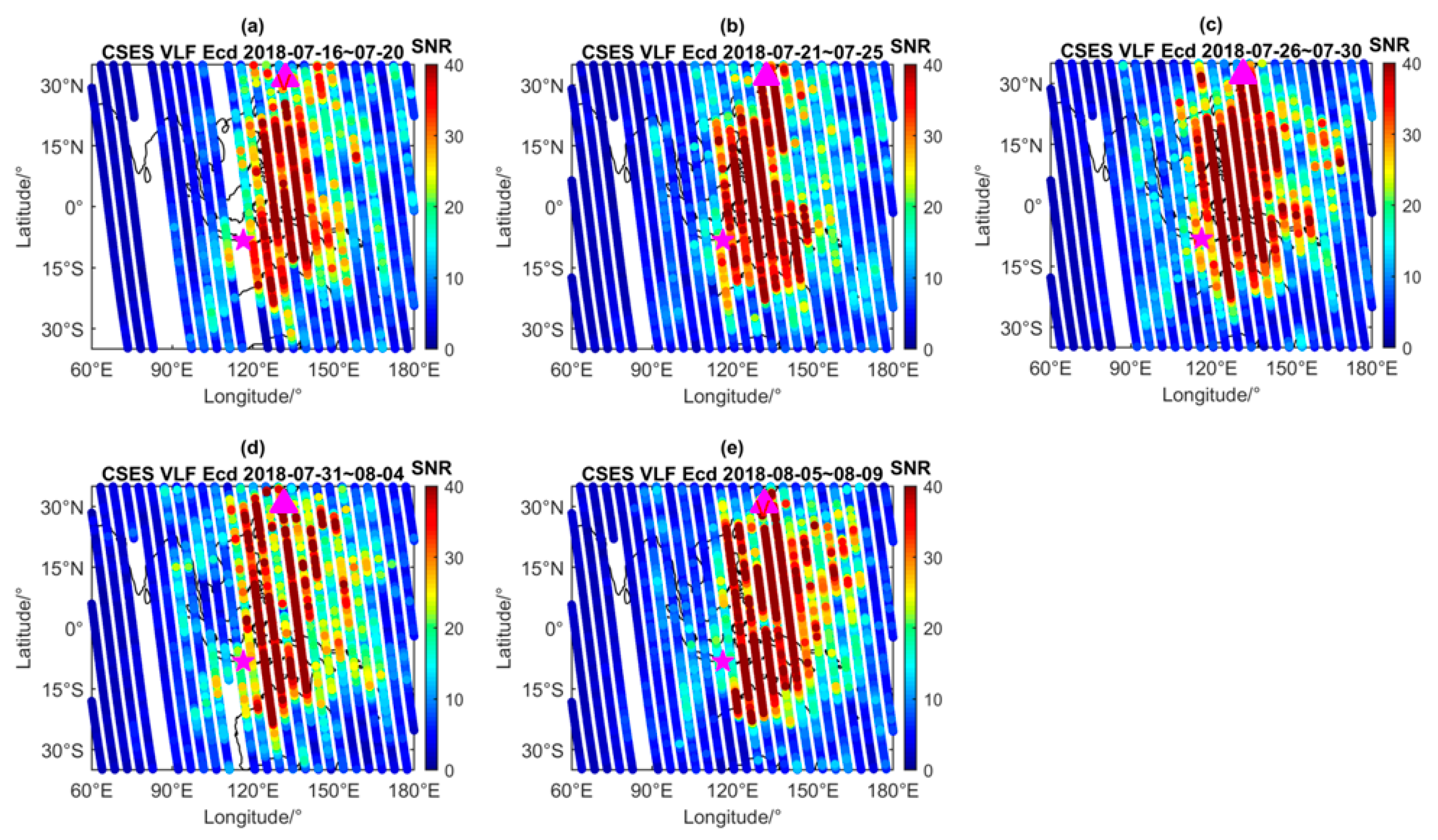
3.2. SNR from JJI at 22.2 kHz

By taking ~±240 Hz as the preferred background, the SNR values were computed at 22.2 kHz for the JJI transmitter in Japan. A large space scale is displayed in Figure 3 at latitudes of ±35° mainly due to the location of JJI. The results show that SNR from JJI with small emitted power of 200 kW almost reduced a half when compared to those from NWC one. Large SNR values were mainly recorded at the east side of the epicenter due to the transmitter longitude of 130.81°E. From the 5 panels of Figure 3, one can see that the lower SNR values, less than 30, occurred almost along the whole orbit at the east side of the epicenter. The lowest ones, less than 20, were detected after the earthquake (see Figure 3e), but large values were observed in the southern part along the orbit. Additionally, the JJI covering the area appears much larger (see Figure 3e) than that during 31 July to 4 August (see Figure 3d). From 31 July to 4 August, lower SNR values were detected along the orbit localized in the middle of the covering area of the JJI transmitter as shown in Figure 3d.

4. Comparison with Other Physical Parameters

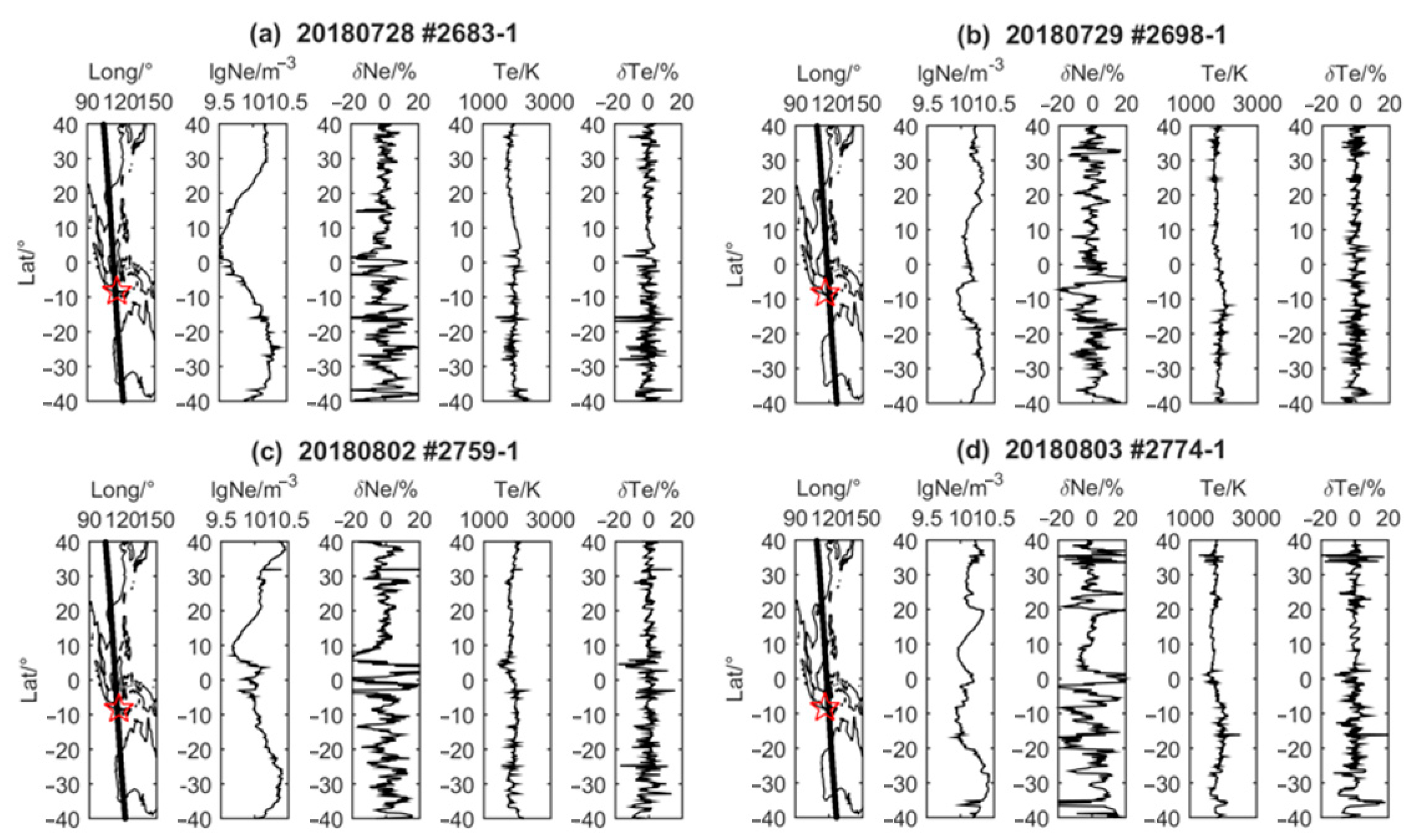
4.1. Electron Density in the Ionosphere

The electron density (Ne) is one of the main factors affecting the propagation and penetration of VLF radio waves, especially during the earthquake-ionosphere coupling processes. Song [35] studied this earthquake by using Ne from the Langmuir Probe (LAP) on CSES, and found huge perturbations in local nighttime along the three orbits, i.e., #2728-1 on 31 July, #2819-1 on 6 August, and #2835-1 on 7 August 2018. As shown in Figure 2c, important differences occurred in the NWC transmitter signal at the east and west sides of the epicenter during 26 to 30 July. Figure 4 displays the electron density (Ne) and the temperature (Te) variations, at both sides, along the two nearest orbits, i.e., #2683-1 on 28 July and #2698-1 on 29 July. On the CSES satellite, the sampling rate of LAP is 3 s in SURVEY mode. We used a 20-point moving average to remove the background and to estimate the relative variation using δNe = (Ne-$\overline{\mathrm{Ne}}$ )/$\overline{\mathrm{Ne}}$ ($\overline{\mathrm{Ne}}$ is the averaged electron density) and δTe, in which the signals above 20% are considered as anomalies. It can be seen that along the west orbit of #2683-1 on 28 July, Ne exhibits lower values of about 109.5 m⁻³ at latitudes of 0–10°N and flat Te about 2000 K (Figure 4a). While along the east orbit #2698-1 on 29 July, Ne is found to be higher than 10¹⁰ m⁻³ above the equatorial area, more than those along the orbit #2683-1. Hence, Ne at the east side of the epicenter is higher than that at the west side, which may result in lower VLF electric fields at the east side, as shown in Figure 2c. To confirm this feature, we show in Figure 4c and Figure 6d the electron density variations along two other orbits, i.e., #2759-1 on 2 August and #2774-1 on 3 August. One should note that the valley Ne moved northward to latitude of 10°N, between ±5° latitudes, where small values were detected in Ne with important perturbations in δNe of about 50%; this is consistent with the decrease in SNR (see Figure 2d) at the equatorial area along this orbit. Along the orbit #2774-1 on 3 August, Ne was still above 10¹⁰ m⁻³ as that along the revisited orbit of #2689-1 on July 29, with broad latitude variations at 20–40°N and −40–0°S. Along this orbit, SNR from NWC did not reduce (see Figure 2d) but from JJI it decreased significantly (see Figure 3d) in both hemispheres. The results from Ne analysis illustrate that large Ne has small SNR, which shows, to some extent, the relationship between the electron density and the electric field SNR variation. However, this feature is not usually observed so we cannot confirm their direct relationship. Besides, it should be noted that Ne studied here is observed at the satellite altitude at about 507 km, and it only represents the plasma environment at the topside ionosphere, not the lower ionosphere that influences the penetration of VLF signals more heavily.

The total electron content (TEC) consists of the electrons in the unit volume between the GPS satellites and the receivers on the ground, which is also usually used in the earthquake research. The global TEC data from JPL (Jet Propulsion Laboratory) were collected around this Indonesia earthquake. The anomaly ∆TEC is derived using the following equation:

$$\Delta \mathrm{TEC}=\{\begin{array}{c}{\mathrm{TEC}}_{\mathrm{i}}-\left({\mathrm{TEC}}_{\mathrm{mi}}+1.5{\mathrm{IQR}}_{\mathrm{iupper}}\right) \hspace{1em}\hspace{1em}\mathrm{TEC}>{\mathrm{TEC}}_{\mathrm{m}}+1.5{\mathrm{IQR}}_{\mathrm{upper}}\hfill \\ 0\hspace{1em}\hspace{1em}\hspace{1em}\hspace{1em}\hspace{1em}{\mathrm{TEC}}_{\mathrm{m}}-1.5{\mathrm{IQR}}_{\mathrm{lower}}\le \mathrm{TEC}\le {\mathrm{TEC}}_{\mathrm{m}}+1.5{\mathrm{IQR}}_{\mathrm{upper}}\hfill \\ {\mathrm{TEC}}_{\mathrm{i}}-\left({\mathrm{TEC}}_{\mathrm{mi}}-1.5{\mathrm{IQR}}_{\mathrm{ilower}}\right) \hspace{1em}\mathrm{TEC}<{\mathrm{TEC}}_{\mathrm{m}}-1.5{\mathrm{IQR}}_{\mathrm{lower}}\hfill \end{array},$$

(1)

where the index i indicates the universal time with an interval of two hours (i.e., 0, 02…22 UT), TEC_m is the median values of former 15 days at the same UT, and IQR_upper and IQR_lower are the upper and lower IQR (interquartile range) of the former 15 days, where 1.5 times IQR is selected to limit the upper and lower boundaries. The results show that the typical anomalies occurred on 1, 2, and 3 August in GPS TEC. Figure 5 displays the ∆TEC on 1 August 2018. The enhanced TEC anomaly was detected at the following times (in UT): first 04, and then at 08, 10, and 12, where at 12 UT, the anomalies at the conjugate region were even larger, above 5 TECU, than over the epicentral area. The small negative anomalies occurred in the northern hemisphere, in the time interval 18 to 22 UT. On 2 and 3 August, the TEC enhancement continuously occurred at 22UT on 2 August, between 00 and 10UT on 3 August, and in the interval 02-04UT in the conjugate region. It is important to note that the disturbances in the VLF transmitters and the TEC anomalies were observed on the same days, i.e., 2 and 3 August, despite the difference in the time occurrence. In addition, there were even no TEC anomalies detected over the epicentral area, from 26 to 30 July 2018. On the basis of the TEC analysis, anomalies were detected in the beginning of August, i.e., 1 to 3 August, revealing strong disturbances in ionosphere electron density during these days. However, the disturbance time occurrences in GPS TEC and VLF transmitters on the CSES satellite were quite different, with TEC anomalies mostly occurring in local daytime in the Indonesia region. Actually, strong disturbances in Ne were observed from CSES at the equatorial region in the latitude range between −5°S and 20°N on 31 July and 1 August along the closest orbits to the epicenter, while a typical SNR decrease was found on 1 August in the vicinity of the JJI transmitter covering area (see Figure 3d). Just from the TEC and VLF transmitter investigations, it is hard to conclude on the relationship between TEC anomalies and SNR disturbances.

4.2. DC-ULF Electric Field and ion Drift Velocity

The movement of electrons and ions in the ionosphere is closely related to the electric field due to the effects of $\mathrm{E}\times \mathrm{B}$. The same orbits, as in Figure 4, were considered in ULF band using the EFD instrument onboard CSES with a sampling rate of 125 Hz. Small-amplitude modulations were detected after the smoothing and averaging of the ULF electric field along the following orbits, 28–29 July, and 2–3 August, just as those in Ne (see Figure 4). To compare the difference in the electric field, the orbits on 28 and 29 July and 1 and 3 August, were selected, in which 2560 points (about 20 s) were used to derive the remaining disturbances in three components. As shown in Figure 6a,b, along the orbits of #2683-1 and #2698-1, small-amplitude modulations were detected, just as those in δNe in Figure 3. While along the orbits #2743-1 on 1 August and #2774-1 on 3 August, significant differences were found, in which strong perturbations occurred along #2743-1 with a large amplitude of ±100mV/m (Figure 6c), two orders in magnitude bigger than that along #2774-1 of ±2–5mV/m. The two orbits observed the disturbed electric field signals. As shown in Figure 3, on both orbits, one can see a significant SNR decrease above the JJI transmitter region and the epicentral area. However, no specific and confirmed disturbances, on both orbits, can be correlated to the SNR decreases from the electric field taking into consideration the satellite positions or the amplitude of abnormal signals. Hence, the disturbances in the electric field, like the electron density, may not lead to the SNR decrease but to some intermediate developments in the coupling processes.

Onboard CSES, the scientific payload PAP detects the ion-related parameters, including ion drift velocity. Hereafter, four parameters were collected, such as Vx, Vy, Vz, and also the ion fluctuation δNi, where +X points to the satellite flight direction in the satellite coordinate system, +Z is vertically downward, and +Y is perpendicular to the XZ plane according to the right-rotated rule. Due to some contaminations on this payload, some measurements cannot be used, in which the absolute values are not reliable. However, considering its continuous and stable observing state, we mainly analyzed its relative variations among revisited orbits. Figure 7 shows the derived physical parameters, along five orbits similar to those considered in Figure 4 and Figure 6. Comparing the revisited orbits of #2683-1 and #2759-1 in Figure 7 (black and purple lines), a typical decrease was detected in Vx, and an obvious increase occurred along #2759-1 on 2 August in Vz at the southern hemisphere (0–30°S) and Vy at the northern hemisphere (0–30°N) when the ion fluctuations mainly distributed at the southern hemisphere as Vx and Vz. Along the other revisited orbits, i.e., of #2698-1 and #2774-1 (blue and red lines in Figure 7), the enhanced movement in Vz was detected at southern latitudes and an increase of about 10% in δNi along #2774-1 on 3 August. Additionally, the ion drift velocity was enhanced in the −X direction at the southern hemisphere or along almost the whole orbit of #2698-1, #2759-1, and #2774-1 when compared to the orbit #2683-1 on 28 July. While Vy turned to positive values at the northern hemisphere for all orbits except #2683-1, the upward drift velocity in Vz reduced, and ions even moved downwards along the orbits along #2759-1 and #2774-1 on 2 and 3 August at the southern hemisphere relative to that from #2683-1 as a normal background. The ion velocity variations are found to be related to SNR perturbations (see Figure 2 and Figure 3) above the NWC and JJI transmitter regions, on those three days except 28 July. Figure 7 also shows another orbit, i.e., #2743-1 (yellow line) on 1 August, with strong disturbances like in the ULF electric field (see Figure 6c). In the latitude interval between −10°S and 20°N, the enhancement decrease in Vx and the increases in Vy and Vz were observed in the +Y and +Z directions (yellow line in Figure 7). Additionally, from the ion modulation, it varied significantly in a larger scale of latitudes from −20°S to 20°N compared to any other orbits. All these phenomena illustrate the abnormal ion movements in the horizontal and vertical downward directions relative to the normal state on 28 July.

4.3. The Lower Ionosphere Height

The VLF radio waves are well known to propagate over long distances within the Earth-Ionosphere waveguide between the surface and the lower ionosphere. The first nighttime cut-off frequency can be distinguished around 1.7 kHz with a minimum spectrum in the electric field on the CSES satellite, and then the reflection height can be calculated by the equation of $f_c=c/2h$ [36], where c is the light speed of 3 × 10⁸ m/s in the vacuum. Firstly, we considered the VLF electric field spectra, then looked for the corresponding frequency fc with the minimum value in the electric field spectra within the frequency band of 1.2 to 2.3 kHz, and finally obtained the ionosphere height by the above equation: h = c/2f_c. Figure 8 displays the ionosphere heights, in the period from 16 July to 9 August with a time interval of 5 days, as those in Figure 2 and Figure 3. It can be seen that the ionosphere height was mostly about 95 km in the southern hemisphere between 16 and 25 July (Figure 8a,b). It is lower than 90 km over the epicenter region (Figure 8c,d) from 26 July to 4 August. After the earthquake, between 5 and 9 August, it particularly recovered in the eastern region of the epicenter (Figure 8e). It comes that 10 days before the Indonesia earthquake, the lower ionosphere height was reduced by about 10 km in some specific areas, typically from 31 July to 4 August (Figure 8d). Like SNR disturbances, the local ionosphere height also dropped in a relatively larger scale before the earthquake occurrence. The time period and regions with anomalies in SNR and ionosphere height are consistent with each other.

5. Discussion

Several papers have reported about the perturbations in signals emitted by VLF transmitters during the earthquake preparation process. In this investigation, we show similar disturbances in the NWC and JJI transmitter signals onboard the CSES satellite about 10 days before the Indonesia earthquake on 5 August 2018. This result has been confirmed by other physical parameters onboard the same satellite, like Ne, ULF, and ionosphere height, and also GIM TEC. This multi-parameter approach, as discussed in this section, leads to the combination of the recorded anomalies and to an emphasis is on the observation complementary towards a better comprehension of the physical process.

First, we tried to find a probable relationship between the drops of the VLF radio wave signals, recorded on satellite, and the anomalies discovered before the Indonesian earthquake occurrence. From the local observations (i.e., above the epicenter region), we find that higher Ne and lower ionosphere height occur in areas with reduced VLF signals where short-time disturbances in Ne, TEC, and ULF may explain such VLF perturbations along these orbits. Here, one notes that δNe and ΔE in ULF exhibited frequently modulations at the same locations. The electron density plays an important role during the penetration and propagation processes of VLF radio waves into the ionosphere. Zhao [34] simulated the propagation process by using the full-wave matrix method in the case of the NWC transmitter, and compared them with the records on the DEMETER satellite. The authors pointed out that a higher electron density below 250 km will have a significant attenuation on the electromagnetic wave energy, which explains the huge differences between dayside and nightside VLF signals on the satellite [34]. In this research, we only obtained the in situ electron density at the altitude of CSES, i.e., 507 km, where TEC corresponds to the peak values of the ionosphere at about a 350-km height, so both cannot be considered as directly related to the VLF signals. Furthermore, the short-term disturbances in the electron density and electric field may infer the existence of periodic waves like an acoustic gravity wave. However, it is hard to define, from the present study, which kind of disturbances in the electron density and ULF electric field will contribute to the decrease in the SNR of the VLF signals, because the variations of physical parameters (i.e., Ne and ULF) are not found to be systematically correlated to the VLF perturbations. For instance, the Ne perturbation irregularities, such as those recorded on 28 and 29 July, simultaneously display small-amplitude modulations, but one corresponded to the decrease in SNR along the satellite orbit #2698-1, and one did not. Therefore, it is not possible to prove the electron density role in the SNR decrease due to the higher height of the satellite and its complex variations.

In the case of the lower ionosphere height, Toledo-Redondo [37] obtained the effective height on the basis of the first cut-off frequency by using VLF electric field data from DEMETER at a 700-km altitude during 2006–2010. The ionosphere height arose to about 100 km, 5–10 km higher than its surrounding areas from June to August, at latitudes of about ±30° and longitudes between 90° and 150°. Samanes [38] studied its nighttime features at the equatorial region for the western longitudes by using data from the DEMETER satellite and ground VLF receivers, and they found typical seasonal characteristics with lower values in winter time compared to summer time. The effective height in the Indonesia seismic area, as derived in our study, should increase or maintain a relatively high value during July and August, according to [37] and [38]. The decrease of the ionosphere height as estimated in this study is not consistent with the seasonal features. Combined with the reduced upward movement in ions, one comes to the fact that Ne increases in the lower ionosphere. The main supply factor in the decrease of the ionosphere height in the night local time is the lightning activity. Previous simulations for the changes in ionosphere heights were mostly used to explain the TT drift in ground VLF observations before earthquakes [20,21,22].

Three channels were suggested by Hayakawa [39,40] to explain the lithosphere–ionosphere coupling mechanism, including (1) chemical, (2) acoustic, and (3) electromagnetic channels. The first channel is related to the geochemical parameters, which result in the ionospheric modification through the atmospheric electric field. The second one is, on the basis of atmospheric oscillations, induced in the seismo-active region, to propagate up to the ionosphere. The third one is always thought to be insufficient due to the weak intensity of radio emissions generated in the earthquake preparation zone. In this case, the disturbances were detected in the Ne and ULF electric field, along the CSES orbits near the epicenter, so the first channel is suggested to explain them. However, we should note that the electric field is more difficult to interact with the ionosphere at low latitudes than at high latitudes because the seismic region is localized near the equatorial area [41]. Despite this, the electric field disturbances detected by the CSES satellite at low latitudes were higher, at least a few mV/m, comparable to those recorded around earthquakes by the DEMETER satellite [42]. Derived from simulation [37], the overlapped electric field is only few μV/m at the CSES altitude over the seismic region. It is proposed to have another electric field, which originates from the movements of electrons or ions. Considering the strong effects over the large seismic preparation area and its magnetic conjugate region observed by CSES and other experiments, the third mechanism more possibly contributes to change, in this case, the penetration and the propagation of VLF waves into the ionosphere. The reasons for the decrease of the ionosphere height are mainly associated to the lightning activity and the accumulation of neutral gases at the higher atmosphere, such as NO, O₃, and so on. On the basis of the lightning maps in the regions of Indonesia and Australia (http://www.lightningmaps.org/), the averaged stroke density decreased slowly from June to August in 2018; this parameter can be excluded in the coupling mechanism over the Indonesia region. About the ozone distribution, we checked the data published by NASA (https://ozonewatch.gsfc.nasa.gov/), and we found that the ozone content was a little higher on 26–29 July and 5–6 August but lower than 2σ from 16 July to 9 August 2018. Another path to change the ionospheric height in a large scale is the acoustic gravity waves (AGWs), the second channel as suggested by Molchanov [17]. Piersanti [24] used the multi data, including atmospheric temperature, TEC, EFD, and LAP data, on CSES to illustrate the existence of AGWs 6 h before this Indonesia earthquake and the co-seismic effects, and they modeled the field line resonance by an atmospheric pressure gradient caused by a seismic event. Their results demonstrated the occurrence of AGWs before this Indonesia earthquake, which help us to connect the multi experiments in this paper. The AGWs induced on the surface propagate into the atmosphere, causing an ozone content increase and ionospheric height decrease, disturbing the electrons and ions to move upwards or downwards to construct an overlapped electric field emission in ULF band, and finally influence the penetration of VLF waves to lead to lower values of SNR detected at the satellite height.

In our results, some perturbations were not just located quite near to the epicenter in the electric field and electron density onboard CSES. Two reasons may explain them, in which the first one is that the electromagnetic emissions or chemical radiations always distribute along the seismic faults, more active at both top ends of them, and the other is the effects of $\mathrm{E}\times \mathrm{B}$ in the equatorial area like Indonesia. Here, an upward plasma velocity at −8.2°S is used in the SAMI2 model [43]. The profile of the velocity along the altitude is shown by the following Equation (2), where $\mathrm{E}\times \mathrm{B}$ drift is calculated with the sinusoidal function of V₀ ∗ sin[(t-7)/24], and t is the local time in hour:

$$\mathrm{V}\left(z\right)=\{\begin{array}{c}0 z<150 \mathrm{km}\\ \frac{V_0\left(z-150\right)}{150} 150 \mathrm{km}<z<300 \mathrm{km}\\ V_0 z>300 \mathrm{km}\end{array}.$$

(2)

Two velocity values are as input, 0 and 10 m/s, to do the comparison. Figure 9 presents Ne profiles at a 350-km altitude at UT12:09. With the movement of ions at 10m/s in the ionosphere, the peak Ne at 10°N with V₀ = 0 m/s changes into two peaks at 0° and 20°N respectively. Since the Indonesia region is located at the equatorial area, an overlapped electric field will be induced due to the movement of ions, and the main affected area is at latitudes of −5°S to 25°N, to the magnetic conjugate point at the northern hemisphere. At higher latitudes, Ne increases with small amplitude. To illustrate the effects of ion movement, the Fejer empirical model [44] is also employed to get the Ne profile at the same time and altitude (blue color in Figure 9), where no double peaks have been produced. Additional ion movement over the epicentral area will significantly enhance the equatorial anomaly to double peaks. It helps us to understand the spatial distribution features of ionospheric perturbations in parameters, such as TEC, Ne, and electric field, and sometimes the conjugate region effects.

6. Conclusions

The main outcomes from the analysis of multi parameters recorded by the CSES satellite two/three weeks before the occurrence of the Indonesia earthquake on 5 August 2018 are summarized in the following:

(1)

Significant decrease in SNR from the NWC and JJI transmitter signals 10 days before the Indonesia earthquake;

(2)

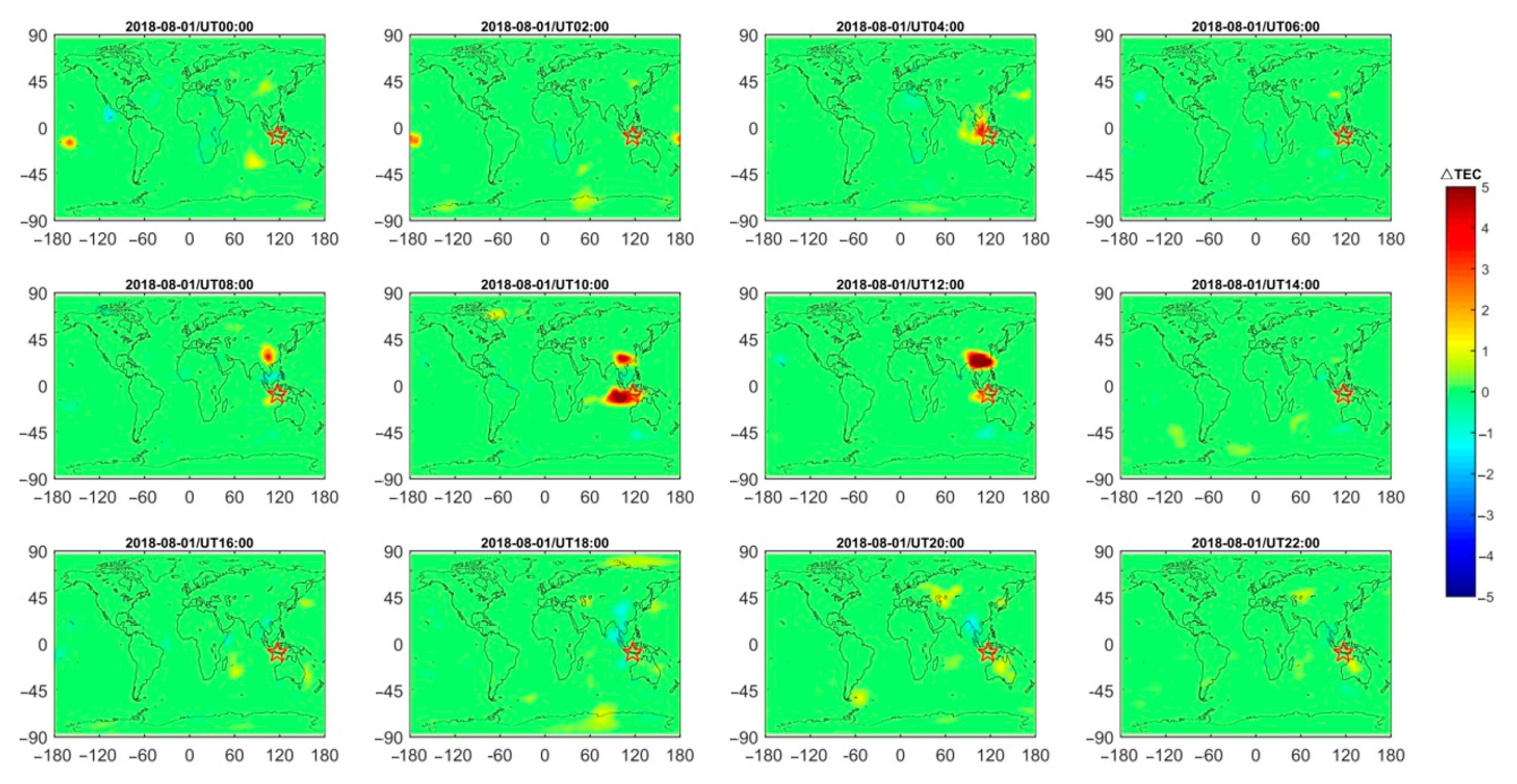
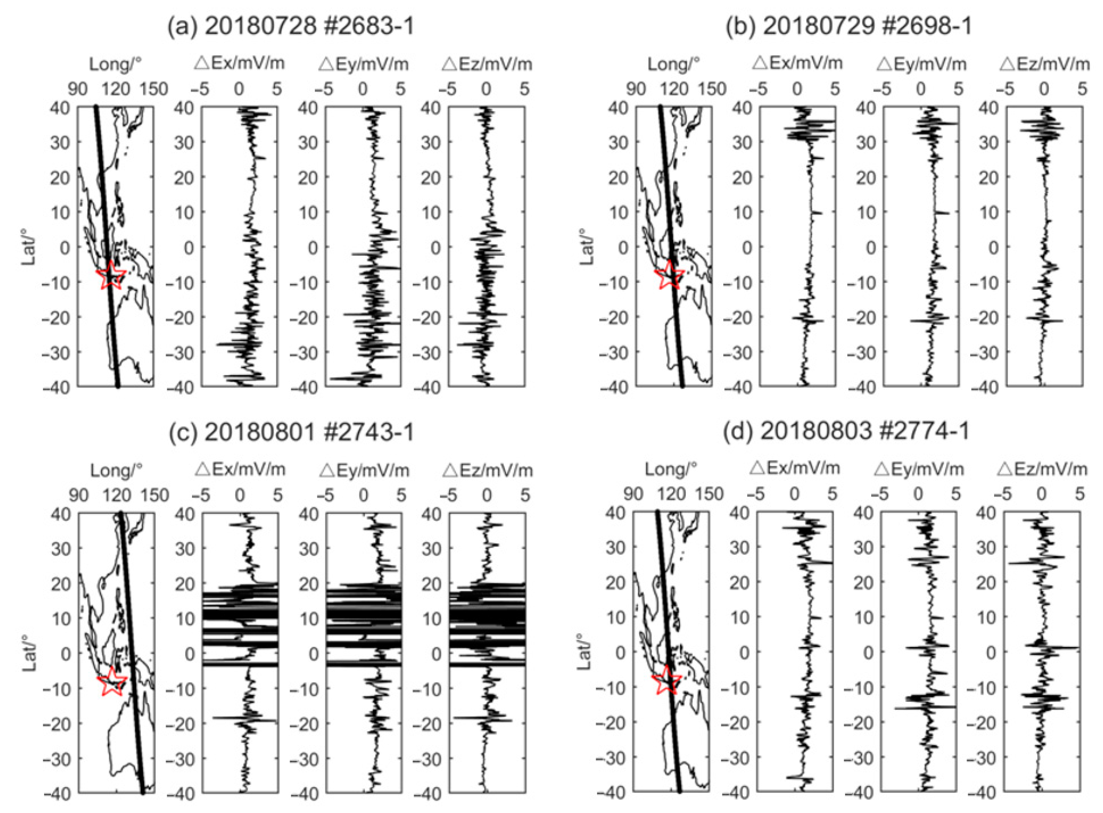
Simultaneous disturbances have been found in the electron density and ULF electric field recorded onboard CSES, and sometime on the same day in GPS TEC from NASA/JPL;

(3)

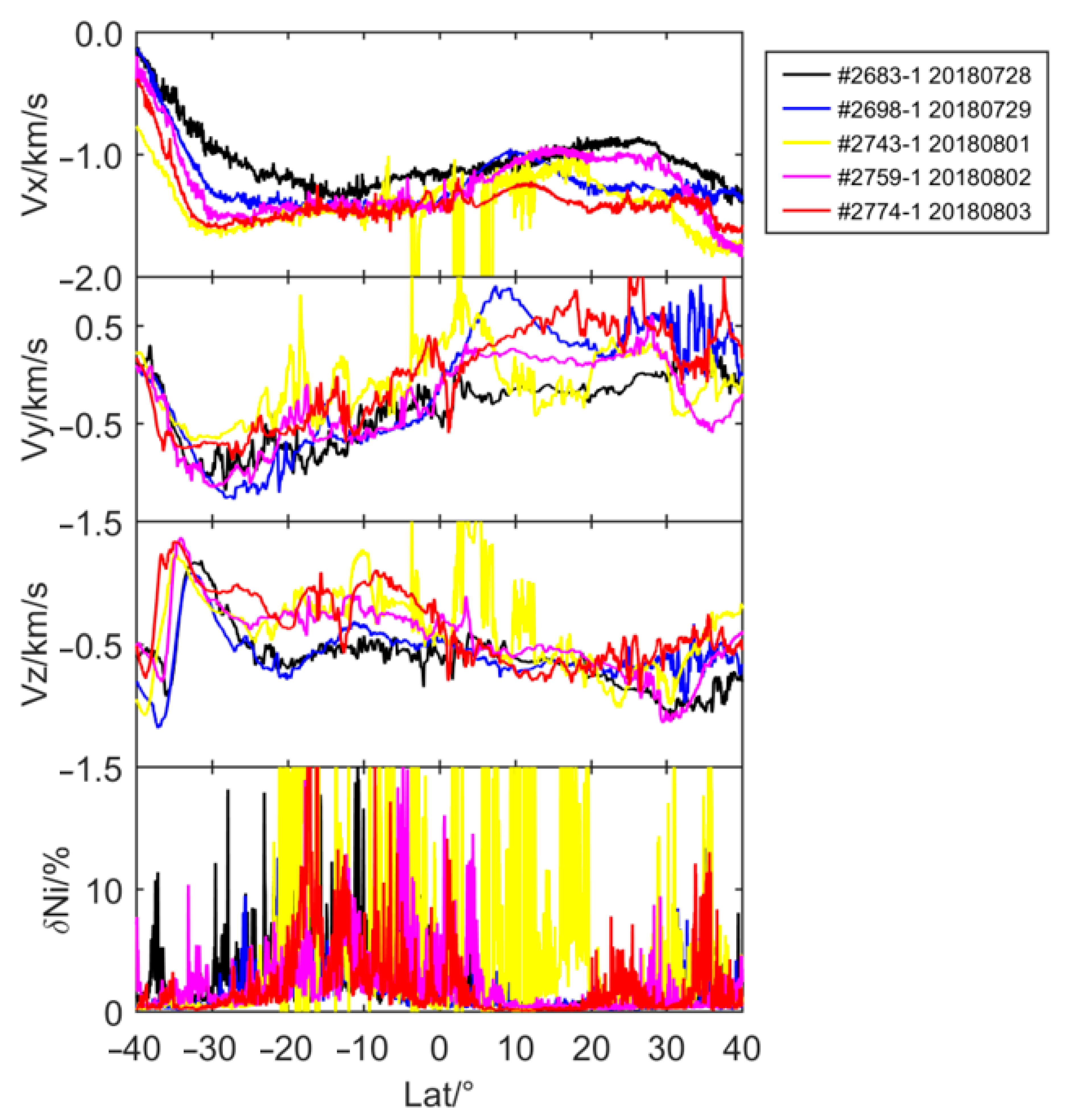
Enhancement of the ion horizontal movements and their upward decelerated movement along orbits with a decrease in SNR;

(4)

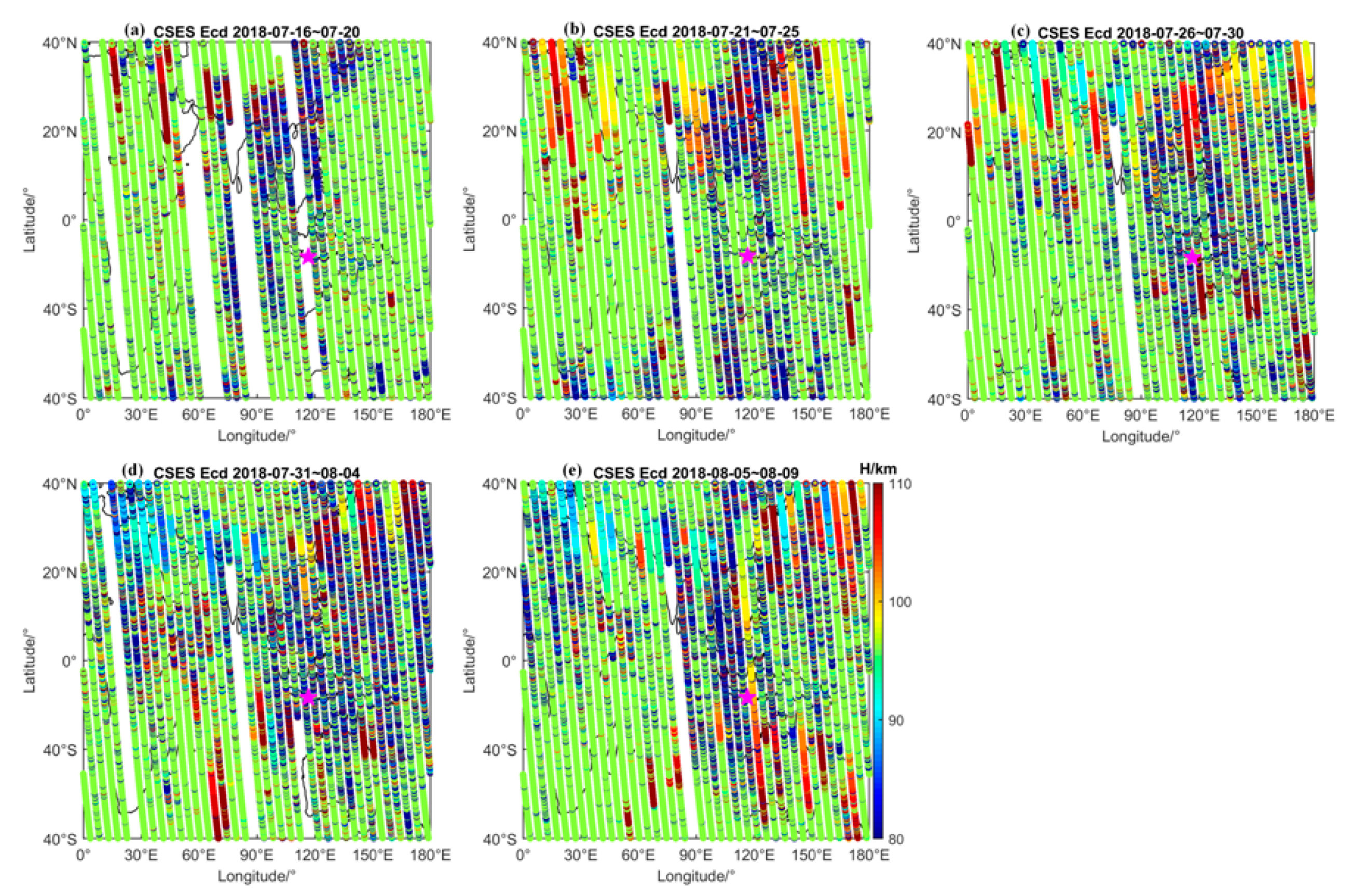
The lower ionosphere height around the epicenter area reduced during 26 July to 9 August at 85 km relative to those during 15 to 25 July at 95 km; and

(5)

The multi-parameter investigations suggest the presence of an overlapped electric field driven by AGWs in the coupling processes from the lower ionosphere to the topside. It results in a series of perturbations in the atmospheric and ionospheric parameters.

References

1. Hayakawa, M. Earthquake Prediction with Radio Techniques; John Wiley and Sons: Singapore, 2015. [Google Scholar]
2. Parrot, M. DEMETER satellite and detection of earthquake signals. In Natural Hazards Earthquakes, Volcanoes, and Landslides; Singh, R., Bartlett, D., Eds.; CRC Press: Boca Raton, FL, USA, 2018; pp. 115–138. [Google Scholar]
3. Helliwell, R.A. Whistlers and Related Ionospheric Phenomena; Stanford University Press: Stanford, CA, USA, 1965. [Google Scholar]
4. Zhao, S.; Shen, X.; Zhang, X.; Pan, W. Full wave calculation of VLF waves penetrated into satellite altitude ionosphere. Chin. J. Space Sci. 2015, 35, 178–184, (In Chinese with English abstract). [Google Scholar] [CrossRef]
5. Cohen, M.B.; Inan, U.S.; Paschal, E.W. Sensitive broadband ELF/VLF radio reception with the AWESOME instrument. Geosci. Remote Sens. IEEE Trans. 2010, 48, 3–17. [Google Scholar] [CrossRef]
6. Chen, Y.; Yang, G.; Ni, B.; Zhao, Z.; Gu, X.; Zhou, C.; Wang, F. Development of ground-based ELF/VLF receiver system in Wuhan and its first results. Adv. Space Res. 2016, 57, 1871–1880. [Google Scholar] [CrossRef]
7. Parrot, M. DEMETER observations of manmade waves that propagate in the ionosphere. Comptes Rendus Phys. Elsevier Masson 2018, 19, 26–35. [Google Scholar] [CrossRef]
8. Chakrabarti, S.K.; Saha, M.; Khan, R.; Mandal, S.; Acharyya, K.; Saha, R. Possible detection of ionospheric disturbances during the Sumatra-Andaman islands earthquakes of December, 2004. Indian J. Radio Space Phys. 2005, 34, 314–318. [Google Scholar]
9. Hayakawa, M. VLF/LF radio sounding of ionospheric perturbations associated with earthquakes. Sensors 2007, 7, 1141–1158. [Google Scholar] [CrossRef] [Green Version]
10. Horie, T.; Yamauchi, T.; Yoshida, M.; Hayakawa, M. The wave-like structures of ionospheric perturbation associated with Sumatra earthquake of 26 December 2004, as revealed from VLF observation in Japan of NWC signals. J. Atmos. Sol. Terr. Phys. 2007, 69, 1021–1028. [Google Scholar] [CrossRef]
11. Hayakawa, M.; Hobara, Y.; Yasuda, Y.; Yamaguchi, H.; Ohta, K.; Izutsu, J.; Nakamura, T. Possible precursor to the March 11, 2011, Japan earthquake: Ionospheric perturbations as seen by subionospheric very low frequency/low frequency propagation. Ann. Geophys. 2012, 55, 95–99. [Google Scholar] [CrossRef]
12. Cohen, M.B.; Marshall, R.A. ELF/VLF recordings during the 11 March 2011 Japanese Tohoku earthquake. Geophys. Res. Lett. 2012, 39, L11804. [Google Scholar] [CrossRef]
13. Ghosh, S.; Chakraborty, S.; Sasmal, S.; Basak, T.; Chakrabarti, S.K.; Samanta, A. Comparative study of the possible lower ionospheric anomalies in very low frequency (VLF) signal during Honshu, 2011 and Nepal, 2015 earthquakes. Geomat. Nat. Hazards Risk 2019, 10, 1596–1612. [Google Scholar] [CrossRef] [Green Version]
14. Rozhnoi, A.; Solovieva, M.; Hayakawa, M.; Yamaguchi, H.; Hobara, Y.; Levin, B.; Fedun, V. Tsunami-driven ionospheric perturbations associated with the 2011 Tohoku earthquake as detected by subionospheric VLF signals. Geomat. Nat. Hazards Risk 2014, 5, 285–292. [Google Scholar] [CrossRef] [Green Version]
15. Maurya, A.K.; Venkatesham, K.; Tiwari, P.; Vijaykumar, K.; Singh, R.; Singh, A.K.; Ramesh, D.S. The 25 april 2015 Nepal earthquake: Investigation of precursor in VLF subionospheric signal. J. Geophys. Res. Space Phys. 2016, 121, 10403–10416. [Google Scholar] [CrossRef] [Green Version]
16. Phanikumar, D.V.; Maurya, A.K.; Kumar, K.N.; Venkatesham, K.; Singh, R.; Sharma, S.; Naja, M. Anomalous variations of VLF sub-ionospheric signal and mesospheric ozone prior to 2015 Gorkha Nepal earthquake. Sci. Rep. 2018, 8, 9381. [Google Scholar] [CrossRef] [PubMed] [Green Version]
17. Molchanov, O.A.; Rozhnoi, A.; Solovieva, M.; Akentieva, O. Global diagnostics of the ionospheric perturbations related to the seismic activity using the VLF radio signals collected on the DEMETER satellite. Nat. Hazards 2006, 6, 745–753. [Google Scholar] [CrossRef]
18. He, Y.F.; Yang, D.M.; Chen, H.R.; Qian, J.D.; Zhu, R.; Parrot, M. SNR changes of VLF radio signals detected onboard the DEMETER satellite and their possible relationship to the Wenchuan earthquake. Sci. China Ser. D Earth Sci. 2009, 52, 754–763. [Google Scholar] [CrossRef]
19. Zhang, X.; Zhao, S.; Song, R.; Zhai, D. The propagation features of LF radio waves at topside ionosphere and their variations possibly related to Wenchuan earthquake in 2008. Adv. Space Res. 2019, 63, 3536–3544. [Google Scholar] [CrossRef]
20. Hayakawa, M.; Molchanov, O.A.; Ondoh, T.; Kawai, E. The precursory signature effect of the Kobe earthquake on VLF subionospheric signals. J. Commun. Res. Lab. 1996, 43, 169–180. [Google Scholar]
21. Rodger, C.; Clilverd, M. Modeling of subionospheric VLF signals perturbations associated with earthquakes. Radio Sci. 1999, 34, 1177–1185. [Google Scholar] [CrossRef] [Green Version]
22. Chakraborty, S.; Sasmal, S.; Basak, T.; Ghosh, S.; Palit, S.; Chakrabarti, S.K.; Ray, S. Numerical modeling of possible lower ionospheric anomalies associated with Nepal earthquake in May, 2015. Adv. Space Res. 2017, 60, 1787–1796. [Google Scholar] [CrossRef]
23. Lizunov, G.; Skorokhod, T.; Hayakawa, M.; Korepanov, V. Formation of ionospheric precursors of earthquakes-probable mechanism and its substantiation. Open J. Earthq. Res. 2020, 9, 142–169. [Google Scholar] [CrossRef] [Green Version]
24. Piesanti, M.; Materassi, M.; Battiston, R.; Carbone, V.; Cicone, A.; D’Angelo, G.; Diego, P.; Ubertini, P. Magnetospheric-ionospheric-lithospheric coupling model. 1: Observations during the 5 August 2018 Bayan earthquake. Remote Sens. 2020, 12, 3299. [Google Scholar] [CrossRef]
25. Rozhnoi, A.; Molchanov, O.; Solovieva, M.; Gladushev, V.; Akentieva, O.; Berthelier, J.J.; Parrot, M.; Lefeuvre, F.; Hayakawa, M.; Castellana, L.; et al. Possible seismo-ionosphere perturbations revealed by VLF signals collected on ground and on a satellite. Nat. Hazards Earth Syst. Sci. 2007, 7, 617–624. [Google Scholar] [CrossRef] [Green Version]
26. Singh, V.; Hobara, Y. Simultaneous study of VLF/ULF anomalies associated with earthquakes in Japan. Open J. Earthq. Res. 2020, 9, 201–215. [Google Scholar] [CrossRef] [Green Version]
27. Parrot, M.; Berthelier, J.J.; Lebreton, J.P.; Sauvaud, J.A.; Santolik, O.; Blecki, J. Examples of unusual ionospheric observations made by the DEMETER satellite over seismic regions. Phys. Chem. Earth Parts A/B/C 2006, 31, 486–495. [Google Scholar] [CrossRef]
28. Liu, J.; Zhang, X.; Novikov, V.; Shen, X. Variations of ionospheric plasma at different altitudes before the 2005 Sumatra Indonesia Ms 7.2 earthquake. J. Geophys. Res. Space Phys. 2016, 121, 9179–9187. [Google Scholar] [CrossRef] [Green Version]
29. Akhoondzadeh, M.; Santis, A.; Marchetti, D.; Piscini, A.; Cianchini, G. Multi precursors analysis associated with the powerful Educator (Mw = 7.8) earthquake of 16 April 2016 using Swarm satellites data in conjunction with other multi-platform satellite and ground data. Adv. Space Res. 2018, 61, 248–263. [Google Scholar] [CrossRef] [Green Version]
30. Shen, X.; Zhang, H.; Yuan, X.; Wang, S.G.; Cao, L.W.; Huang, J.B.; Zhu, J.P.; Piergiorgio, X.H.; Dai, J.P. The state-of-the-art of the China seismo-electromagnetic satellite mission. Sci. China Technol. Sci. 2018, 61, 634–642. [Google Scholar] [CrossRef]
31. Shen, X.H.; Zong, Q.G.; Zhang, X. Introduction to special section on the China seismo-electromagnetic satellite and initial results. Earth Planet. Phys. 2018, 2, 439–443. [Google Scholar] [CrossRef]
32. Zhang, X.; Frolov, V.; Zhao, S.; Zhou, C.; Wang, Y.; Ryabov, A.; Zhai, D. The first joint experimental results between SURA and CSES. Earth Planet. Phys. 2018, 2, 527–537. [Google Scholar] [CrossRef]
33. Zhang, X.; Frolov, V.; Shen, X.; Wang, Y.; Zhou, C.; Lu, H.; Huang, J.P.; Ryabov, A.; Zhai, D.L. The electromagnetic emissions and plasma modulations at middle latitudes related to SURA-CSES experiments in 2018. Radio Sci. 2020, 55, e2019RS007040. [Google Scholar] [CrossRef]
34. Zhao, S.F.; Zhang, X.M.; Zhao, Z.Y.; Shen, X.H.; Zhou, C. Temporal variations of electromagnetic responses in the ionosphere excited by the NWC communication station. Chin. J. Geophys. 2015, 58, 2263–2273, (In Chinese with English abstract). [Google Scholar] [CrossRef]
35. Song, R.; Hattori, K.; Zhang, X.; Sanaka, S. Seismic-ionospheric effects prior to four earthquakes in Indonesia detected by the China seismo-electromagnetic satellite. J. Atmos. Sol. Terr. Phys. 2020, 205, 105291. [Google Scholar] [CrossRef]
36. Cheng, D.K. Field and Wave Electromagnetics; Addison-Wesley Publishing: Reading, MA, USA; Menlo Park, CA, USA, 1989. [Google Scholar]
37. Toledo-Redondo, S.; Parrot, M.; Salinas, A. Variation of the first cut-off frequency of the Earth-ionosphere waveguide observed by DEMETER. J. Geophys. Res. 2012, 117, A04321. [Google Scholar] [CrossRef] [Green Version]
38. Samanes, J.; Raulin, J.P.; Cao, J.B.; Magalhaes, A. Nighttime lower ionosphere height estimation from the VLF modal interference distance. J. Atmos. Sol. Terr. Phys. 2018, 167, 39–47. [Google Scholar] [CrossRef]
39. Hayakawa, M.; Molchanov, O.A. NASDA/UEC team. Summary report of NASDA’s earthquake remote sensing frontier project. Phys. Chem. Earth 2004, 29, 617–625. [Google Scholar] [CrossRef]
40. Hayakawa, M.; Molchanov, O.A. NASDA/UEC team. Achievements of NASDA’s earthquake remote sensing frontier project. Terr. Atmos. Ocean. Sci. 2004, 15, 311–328. [Google Scholar] [CrossRef] [Green Version]
41. Zhou, C.; Liu, Y.; Zhao, S.F.; Liu, J.; Zhang, X.M.; Huang, J.P.; Shen, X.H.; Ni, B.B.; Zhao, Z.Y. An electric field penetration model for seismo-ionospheric research. Adv. Space Res. 2017, 60, 2217–2232. [Google Scholar] [CrossRef]
42. Zhang, X.; Shen, X.; Zhao, S.; Yao, L.; Ouyang, X.; Qian, J. The characteristics of quasistatic electric field perturbations observed by DEMETER satellite before large earthquakes. J. Asian Earth Sci. 2014, 79, 42–52. [Google Scholar] [CrossRef]
43. Huba, J.D.; Joyce, G.; Fedder, J.A. Sami2 is another model of the ionsopehre (SAMI2): A new low-latitude ionosphere model. J. Geophys. Res. 2000, 105, 23. [Google Scholar]
44. Scherliess, L.; Fejer, B. Radar and satellite global equatorial F region vertical drift model. J. Geophys. Res. 1999, 104, 6829. [Google Scholar] [CrossRef]
Figure 1. The power spectrum density in Ead along the orbits of #2516-1 and #2546-1 (from top to bottom: the spectra at frequency band of 18 to 23 kHz along the orbit, the spectrum at fixed frequency 20.5 (second left-panel) or 20.4 kHz (second right-panel) along the latitude, and the spectrum at a given latitude −8.2°S in the frequency range 15–25 kHz.
Remotesensing 12 04050 g001
Figure 2. The SNR distributions of Ecd from NWC in local nighttime during 16 July to 9 August in 2018 around the earthquake (a): 17–20 July; (b): 21–25 July; (c): 26–30 July; (d): 31 July–4 August; (e): 5–9 August; : epicenter; : NWC transmitter; the color bar presents the values of SNR).
Remotesensing 12 04050 g002
Figure 3. The SNR distributions of Ecd from the JJI transmitter around the earthquake area (a): 17–20 July; (b): 21–25 July; (c): 26–30 July; (d): 31 July–4 August; (e): 5–9 August; : epicenter; : JJI transmitter; the color bar presents the values of SNR.
Remotesensing 12 04050 g003
Figure 4. The electron density (Ne) and temperature (Te) and their relative variations in δNe and δTe along four orbits (a): #2683-1 on 28 July; (b): #2698-1 on 29 July; (c): #2759-1 on 2 August; (d): #2774-1 on 3 August; : epicenter).
Remotesensing 12 04050 g004
Figure 5. Global GPS TEC anomalies (∆TEC) in two hours from 00UT to 22UT on 1 August 2018 (: epicenter).
Remotesensing 12 04050 g005
Figure 6. The disturbance in three components of the ULF electric field ((a) orbit #2683-1 on 28 July, (b) orbit #2698-1 on 29 July, (c) orbit #2743-1 on 1 August, (d) orbit #2774-1 on 3 August 2018).
Remotesensing 12 04050 g006
Figure 7. The variations of the ion drift velocity (Vx, Vy, Vz) and ion fluctuation (δNi), along five orbits, as recorded by PAP instrument onboard CSES.
Remotesensing 12 04050 g007
Figure 8. The ionosphere height variation in the 5-day interval from 16 July to 9 August 2018. (: epicenter, (a) 16–20 July, (b) 21–25 July, (c) 26–30 July, (d) 31 July–4 August, (e) 5–9 August 2018).
Remotesensing 12 04050 g008
Figure 9. Ne profiles at a 350-km altitude around UT12 driven by two velocity values (0m/s with black color and 10m/s in red).
Remotesensing 12 04050 g009