Navigation and Mapping in Forest Environment Using Sparse Point Clouds
by
 , ,
, ,
Paavo Nevalainen
1,*, 
Qingqing Li
1,
Timo Melkas
2,
Kirsi Riekki
2,
Tomi Westerlund
1 and
Jukka Heikkonen
1 1
Department of Future Technologies, University of Turku, 20014 Turku, Finland
2
Metsäteho Oy, 01300 Vantaa, Finland
*
Author to whom correspondence should be addressed.
Remote Sens. 2020, 12(24), 4088; https://0-doi-org.brum.beds.ac.uk/10.3390/rs12244088
Submission received: 9 November 2020
/
Revised: 6 December 2020
/
Accepted: 9 December 2020
/
Published: 14 December 2020
(This article belongs to the Special Issue 3D Point Clouds in Forest Remote Sensing)
Abstract
:Odometry during forest operations is demanding, involving limited field of vision (FOV), back-and-forth work cycle movements, and occasional close obstacles, which create problems for state-of-the-art systems. We propose a two-phase on-board process, where tree stem registration produces a sparse point cloud (PC) which is then used for simultaneous location and mapping (SLAM). A field test was carried out using a harvester with a laser scanner and a global navigation satellite system (GNSS) performing forest thinning over a 520 m strip route. Two SLAM methods are used: The proposed sparse SLAM (sSLAM) and a standard method, LeGO-LOAM (LLOAM). A generic SLAM post-processing method is presented, which improves the odometric accuracy with a small additional processing cost. The sSLAM method uses only tree stem centers, reducing the allocated memory to approximately 1% of the total PC size. Odometry and mapping comparisons between sSLAM and LLOAM are presented. Both methods show 85% agreement in registration within 15 m of the strip road and odometric accuracy of 0.5 m per 100 m. Accuracy is evaluated by comparing the harvester location derived through odometry to locations collected by a GNSS receiver mounted on the harvester.
1. Introduction
Modern Cut-to-length (CTL) harvesters [1] cut, delimb and buck the stem to the different timber assortments at the work site. These timber assortments are then delivered to the roadside by forwarders. There exists a high demand for automation, especially for autonomous micro-tasks [2], which would speed up the work cycles and improve overall quality. These micro-tasks and the following short-range logistics require situational awareness [3] and data synchronization between the harvester and the forwarder.
A tree map is a collection of geographic tree locations and stem properties, such as the diameter at breast height (DBH), branch height, and stem profile, which can serve as a bridge between on-ground mapping [4] and aerial mapping [5], as well as providing a possible basis for future autonomous or semi-automatic logging operations. For example, temporary timber piles may be located not in somewhat inaccurate global co-ordinates, but in accurate (within 20 cm) local co-ordinates related to nearby trees and other landmarks. Additionally, local tree maps are needed for assisted local movement planning. In this field, two co-ordinate systems are mainly used: Global Navigation Satellite System (GNSS) and the local co-ordinates defined by the tree trunks. These are fused, whenever possible, and there are only two extreme cases where this is difficult: (1) Final cutting in an environment with a monotonic ground profile, where only GNSS can be used by the forwarder; and (2) almost complete canopy cover in a highly rugged environment, where GNSS information becomes erroneous. These two extremities are not considered in this study.
A tree map can be used for autonomous navigation [3], matching with previous data resources such as canopy maps and forest inventories [6], as well as forestry management. Current issues in forest simultaneous location and mapping (SLAM) are the map representation, map permanence (how much to keep in memory and how much to forget and relearn), and adaptations to resource-constrained platforms [7].
A summary of the international research on building forest inventories by terrestrial laser scan (TLS) approaches has been given in [8]. This article stated that the main problems are the redundancy of point cloud (PC) information, on one hand, and incompleteness, on the other hand, making multi-scan approaches, such as those used in this research, difficult to execute properly. Even TLS, which is based on single scans, is very closely related to forest SLAM, especially when some of the scans are rejected to gain more computation time.
The typical speed in forestry operations is rather slow (e.g., a CTL harvester has an operating speed of 0.3–0.8 m/s), which includes harvesting and moving between work cycles. This slow speed allows for sparse frame sampling. Environment and path optimizations dictate parallel strip roads, where large-scale closed loops [9] do not occur very often, but very small work cycle loops (2–5 m) are common.
In the following, methods for detecting trees and the SLAM process are reviewed as potentially separate problems. Some of the methods hold an aspect for both tasks and, as such, are mentioned twice.
1.1. Existing Methods to Detect Tree Stems
The following methods have been presented in the literature for the detection of tree stems from PC views. Some of them have DBH detection built-in, while others include the SLAM and DBH aspects as two separate steps. All of the methods have some recurring heuristic elements and, thus, the following categorization attempts to capture the main strategies:
- Robust cylinder matching to a local density concentration of a horizontally projected PC. Cylinder and circle match techniques have been presented, for example, in [10]. Included is the Hough transform, a heuristic approach composed of several steps including the spectral decomposition of local neighborhoods, a robust cylinder fit, and voxel filtering, followed by random sample consensus (RANSAC). The maximum likelihood approach of [11] also belongs to this group.The local density method was used in [12]. This method should first be adapted to mobile laser scanning tasks and is limited to relatively small ranges (approximately 10 m), due to its high point density requirements. Vertically layered computation is an interesting detail, which can be integrated into many of the other algorithms listed here, though.
- Voxel voting [13] means that a series of morphological operations on voxels reduce the canopy and strengthen the couplings between potential stem voxels. The voxel-based normalized cut of [14] could be adapted to tree stem detection in the case of a low-density TLS. The method presented in [10] also belongs to this category.
- The local filtering of points is based on a geometric feature or a group of them, before progressing to, for example, cylinder matching (see case 1) or line segment matching (case 4). The stem center line segment starts from the approximated ground level and proceeds to the highest hit point of the stem. Such a stem line segment is typically at the minimum square error position related to the points. Local filtering may include a clustering phase, such as a connected component segmentation algorithm [15], which uses local geometric features like curvature. The approach of [15] detected stems well, but was rather inaccurate in DBH measurement and may not be suitable for on-board and online tree map computation.
- Matching a line segment to individual tree stems. This can be, for example, a result of local principal orientations [16] after the final PC has been constructed by the SLAM process or producing a sparse SLAM problem in a preliminary phase.
- Using 3D convolutional neural networks (CNN) detecting tree stems. This approach is often limited either to airborne laser scan (ALS) cases, or to highly dense TLS. Most object registration methods are subjected to the use of sparse PC voxelization as an initial step. A rather simple case of rubber tree stem detection [17] required approximately 800 manually labeled samples. This approach seems conceivable in boreal forests; however, the global diversity of commercially significant forest environments makes training data accumulation a major effort. This suggests a need for versatile methods with auto-calibration properties.
It seems that the real-time or non-real-time construction of a local tree map with limited range (approximately 10–15 m) is possible through the use of many existing methods (e.g., [4,15]) for some environments. Even the inclusion of some trees at the extended range of 15–35 m could improve the angular accuracy of the odometry, thus reducing cumulative errors.
1.2. Existing Real-Time SLAM Methods
One of the earliest applications to a moving platform in a forest environment was presented in [18]. The problem of identifying trees by their registration trace in different frames was described in that study, as well as in our case. The implementation was in Java, and computation was carried out a little slower than real-time.
There exist real-time SLAM methods, such as LOAM (lidar odometry and mapping in real-time) [19], which rely on the detection of point sequence properties in individual channels (i.e., a sort of local roughness), the upper values of which define an edge point, and the lower values indicate planar points. This method works well in built-up environments (smooth planar surfaces) with a relative smoothness of the movement. Unfortunately, the lack of smooth surfaces and the perpetual horizontal swing caused by the harvester work cycle make LOAM methods more inaccurate in forest conditions.
The SLOAM (semantic LOAM) pipeline [20] is a state-of-the-art system based on LOAM, which can be mounted on an unmanned aerial vehicle (UAV) [19]. It is focused on timber inventory assessment, including both the SLAM problem from a 360 view and tree stem diameter estimation from individual frames. The simultaneous matching of local tree and ground features provides estimates for tree height and diameter at breast height (DBH). The trained network is very fast, working at 100 Hz input frequency, but the tree detection range seems to be limited to approximately 15 m. Training requires manual control data of tree diameters. The SLAM location error in a closed loop test seems to be 0.58 m per 100 m over a loop length of 65 m.
SLOAM has been shown to be better, in terms of in odometric accuracy, than LOAM in forest conditions (according to [20]), and on par with generalized-ICP (GICP) [21], an industry standard delivered with the Point Cloud Library (PCL) [22]. Considering the SLOAM implementation and the horizontal PC resolution of 0.25–0.29 (lower number for SLOAM test and higher one for our data), planarity detection becomes impossible at a range of approximately 20 m, as there are only 1–2 hits per tree stem and channel when the mean DBH is approximately 20 cm.
The segmentation part of SLOAM [20] consists of a deep learning (DL) method. Several other DL approaches have been proposed for SLAM. The following are examples with potential for forest conditions. The reinforcement learning scheme of [23] allows for adaptation to new environments without requiring a heavy teaching phase. This requires two adaptations: A reformulation of the problem from 2D to 3D, as large rotations do occur in forest terrain, and some sort of preference to tree stem hits and omission or filtering out of foliage and terrain vegetation hits.
LeGO-LOAM [24] includes a ground model which supports the LOAM process, especially in terms of the vertical orientation accuracy. This method seems to be faster than SLOAM. The ground model suffers in the presence of ground vegetation, but seems to be one of the best forest SLAM methods in existence. We shorten its method name to LLOAM in the text below.
Go-ICP [25] is an excellent tool for sparse SLAM tasks. It guarantees finding the best fit within the search zone. It is slower than typical SLAM, unless the search zone can be set tightly. End conditions (the translation and rotation granularity) are auto-tuned, leaving the search zone definitions as the only parameters. It covers only the matches of one frame pair, such that the accumulation of total transformation matrices has to be implemented separately. Its potential for real-time computation is discussed in Section 4.
A DL method has been used to register tree stems, which may be easily applicable to the on-board harvester situation, which has demand ranges of up to 20–40 m. The neural network-based (NN) semantic tree stem shape model [20] may prove to be especially useful in future research. There is a constant flux of emerging DL approaches for PC object registration [26], some of which may be applied to tree detection in the future. LO-Net [27] is the most promising DL method, which has been tested with the Velodyne HDL-64. One needs to train the DL network with the forest SLAM test run, in order to adapt it to forest conditions. Unfortunately, most DL methods require a very large labeled test set.
SLAM can be used for tree stem detection in many forms. One of the most impressive methods of this kind was proposed in [11], which uses several sensor types and a maximum likelihood formulation to detect cylinders from several consecutive light detection and ranging (LiDAR) channels at a time. This method is limited to rather dense and mature forests, however, due to the cylinder registration, which requires several hits per tree stem.
1.3. Proposed Approach
This article examines the potential of SLAM over sparse PCs created by frame-by-frame tree detection. This is an initial study on the industrial setting, which may provide more options for future forestry automation efforts, benefitting from its modular design in order to gain easy adaptability to a wide variety of environments and methods.
Our focus is on the following problem: Tree stem detection with 16 LiDAR channels available, boreal forest as the environment, and the on-board LiDAR of an industrial harvester with jerky movements and a pivoted chassis, with a work cycle featuring constant large rotations. The harvester has GNSS capability for expressing the local tree maps in global co-ordinates. The tree being processed by the cutting head is a recurring obstruction and tree detection is required to reach a 15 m range. Only the faced trees are registered; there is no view behind the machine. The harvester strip roads are typical of normal operations, with no loops allowing for no easy self-consistency checks.
The intended scheme has two major, independent steps: Frame-by-frame tree detection and a SLAM process based on it. Vertical line segments marking tree stems help to assign local PCs of individual trees for further processing, such as for species detection and branch height. Species detection and branch height steps are outside of the scope of this article, however.
The key question in the proposed scheme is whether the stem segment registration step and the resulting sparse point SLAM problem can be executed accurately and in real-time. Another consideration is having a large enough registration scope.
A combination of strategies 3 and 4 is adopted in this study, in order to produce a sparse PC of the tree stem centers before the actual SLAM process. We compare an ordinary SLAM method, represented by LeGO-LOAM [24], and a sparse SLAM method, implemented by Go-ICP [25], which suits sparse 3D SLAM problems well. We use Go-ICP also in the self-consistency check between adjacent tree maps. The potential for modularity comes by separating the SLAM and DBH registration tasks.
2. Materials and Methods
2.1. Site
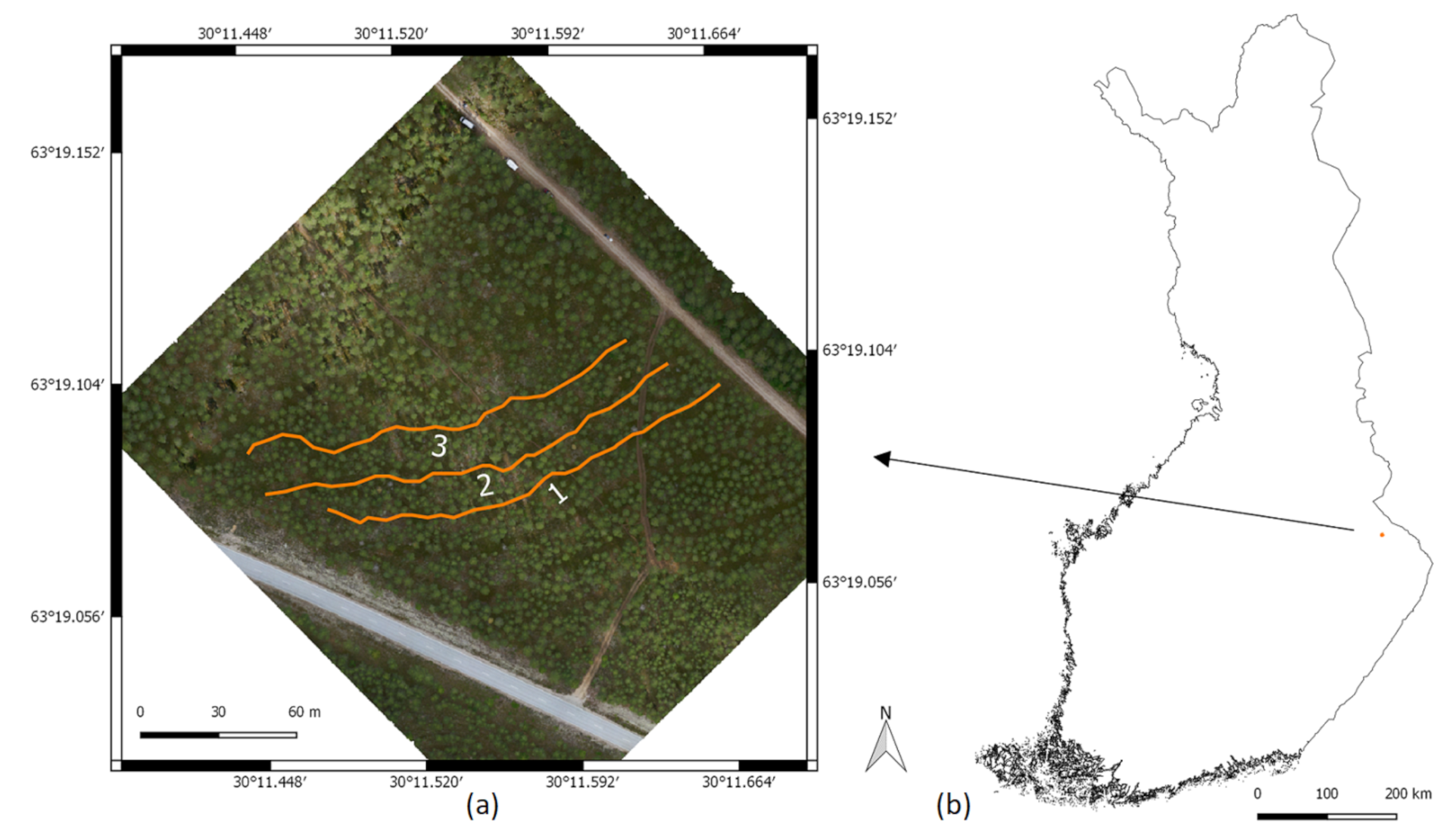
The forest operation site was located in Pankakangas at Lieksa, Eastern Finland (6319.08N, 3011.57E) and the data were captured on August 2017 in co-operation with several participants; see the Acknowledgements section. The location had three strip roads distributed over an area of approximately 60 m × 150 m; see Figure 1.
The study area is part of a mature pine stand (second thinning), with total area of 0.9 ha. The average stand characteristics are: Basal area (G), 16 m/ha; stem volume (V), 120 m/ha; basal area-weighted mean height (Hg), 15 m; and basal area-weighted diameter at breast height (DBH), 18 cm. The average age of trees was 50 years and the stem number was 770 stems/ha. The canopy cover was approximately 55% before thinning. Compared to other regions in Finland, the stand was a typical second thinning. In the laser scanning samples of [28], the site is between “easy” and “medium” difficulty, in terms of tree stem detection. The terrain profile was mostly flat, with the maximum elevation difference over the paths used being 9.3 m.
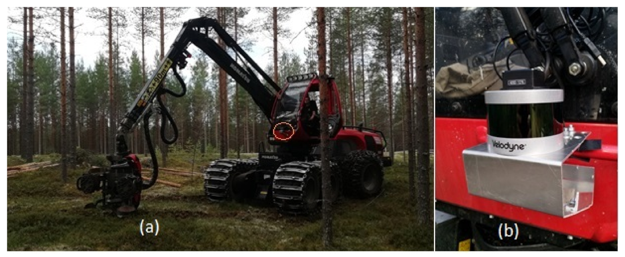
The harvester was a Komatsu Forest 931.1 with a LiDAR unit attached to the front of the cabin at a height of 1.5 m; see Figure 2. The LiDAR view experiences work cycle swings, creating additional difficulty in the SLAM process. The GNSS unit was attached to the roof of the cabin. The cabin was able to rotate 360.
2.2. Data from Various Devices
Point cloud: The Velodyne VLP-16 is a 16 channel LiDAR with 2 cm distance accuracy, 30 vertical view, 2 Hz scanning frequency, and 100 m scan range. The installation provided a horizontal view over 210, while the rest was obscured by the harvester body. A total of 32.7 GB of binary .pcap files were obtained. The scanning rate was 14 frames/s, but only every third frame was recorded, making the processed rate 4.6 frames/s. The practical extreme limit of the scanning range was approximately m. Each individual frame consisted of 10,000–18,000 points with 80–150 visible trees.
GNSS data: G-STAR IV Model no: BU-353S4 was connected to a laptop computer in order to log position data with the corresponding satellite time-stamps and computer time-stamps. The used G-STAR unit recorded 1.2 positions per second. This was equal to 6 cm of movement between positions, on average. Assessment of the actual momentary positional accuracy under a canopy is difficult. The accuracy has quite likely increased from 2015, when it was within a 3.0 m range in forest conditions [29].
Ground model data: A digital elevation model (DEM) has been constructed over two decades through a national programme using aerial laser scanning (ALS). Its vertical error was approximately 0.15 m [30] with a grid size of 2 m. The DEM data were used to verify the height deviation of the odometry.
2.3. Methodology
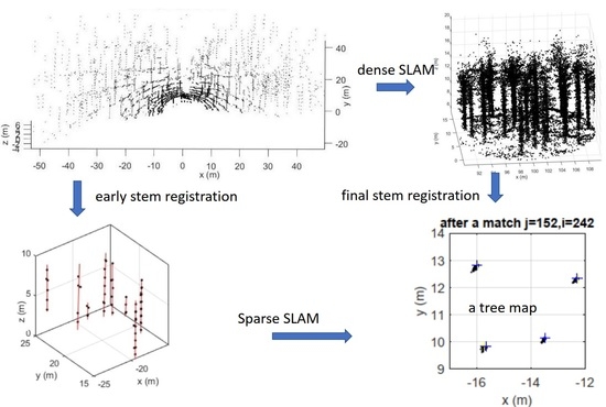
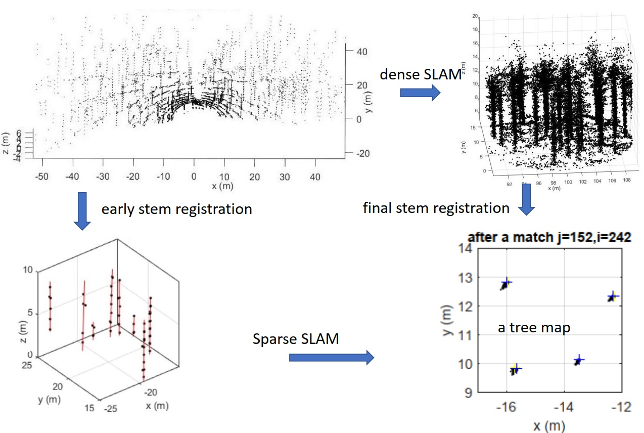
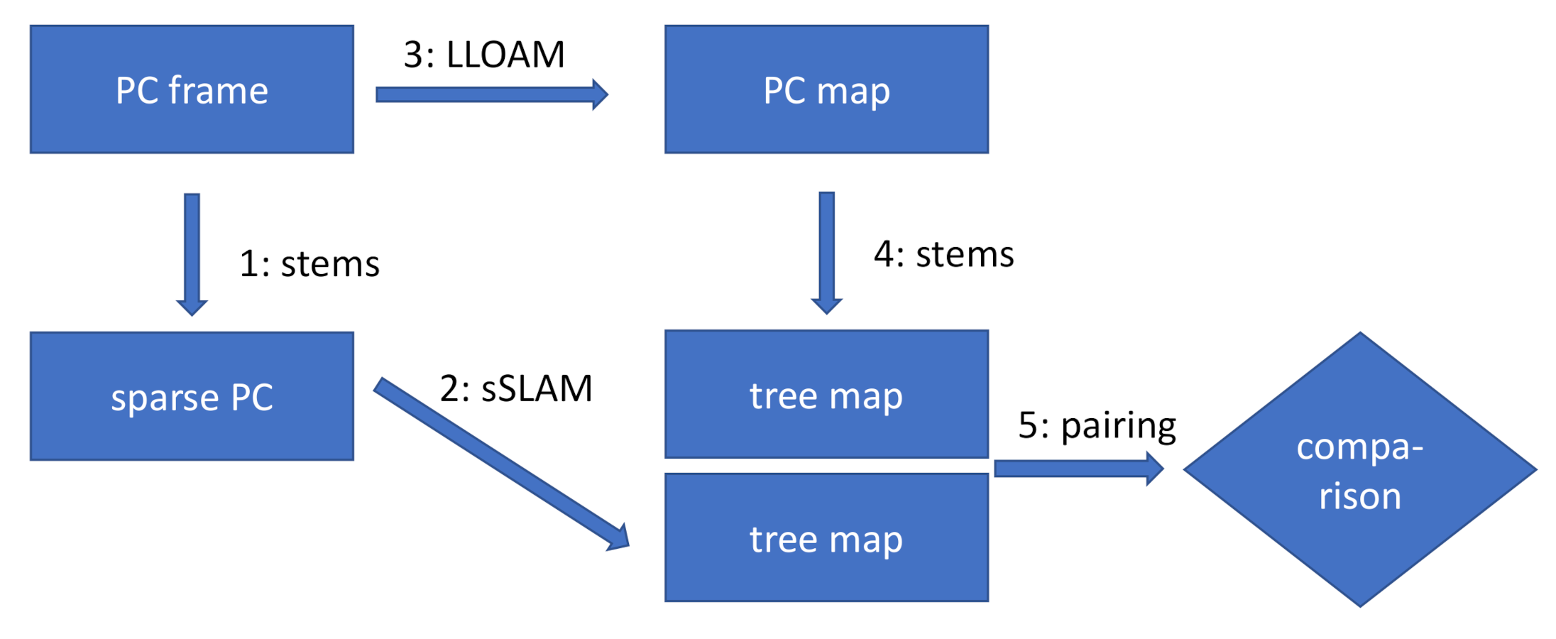
The consecutive steps of the method are introduced in the list below and detailed later in the text. The key idea is to reduce the PC, early on, to a set of tree stem segments in Step 1. Stages 1–6 are listed below and depicted in Figure 3.
- Tree stem detection from frames.
- Sparse SLAM process based on Step 1 and implemented by Go-ICP. [25]. This approach is named sSLAM in the text.
- Conventional dense SLAM by LLOAM, based on Step 1.
- Tree stem detection based on Step 3.
- Comparison of the results by pairing the sSLAM and LLOAM tree maps.
- Matching the odometry path to the GNSS path.
Step 5 involves measuring whether the early stem detection leads to similar accuracy as the late stem detection. In this respect, Steps 1, 3, and 4 have several potential choices for implementation. For convenience, the method described briefly in the following text was used for both Steps 1 and 4, in order to register tree stems.
Tree stem detection: The tree stem detection process is a modular sub-task. It can be any method which succeeds in the frame-by-frame detection of positions of the following Boreal forest species: Scots pine (Pinus sylvestris L.), Norway spruce (Picea abies L. (Karst)), and silver and white/downy birch (Betula pendula (Roth), Betula pubescens (Ehrh.)); that is, any tree species with a relatively straight tree stem. This excludes species like lime tree (Tilia), with more contoured tree stem shape or tendency of low branching. The algorithm developed in this study is included in the supplementary document (see Supplementary Materials). Its design criteria were two-fold:
- Operation on a single frame input with relatively few hits per tree stem and on the final PC map with a dense points.
- Self-calibration capability, in order to avoid parameter tuning requiring a detailed stem map with tree positions and diameters.
Dense SLAM: The LeGO-LOAM [24] method was applied to strip roads 1–3 shown in Figure 1, as described in [3]. The method parameters were set to VLP-16 laser scanner. Computation was carried out after the field campaign, as a separate batch run.
Sparse SLAM The frame-to-frame matching was produced by the Go-ICP algorithm. The only parameter needed was the search scope; in this case, (horizontal and vertical movement, yaw and pitch angles, respectively). The algorithm returns a rigid body transformation t. As a post-processing step, the mean match error, e, of the matched pairs was computed, as well as the ratio of outliers, . The latter is the standard parameter in usual ICP algorithms. Both e and are smallish when a good match is obtained.
An individual match from a frame to occurs by multiplying (points as rows) by a 4 × 4 matrix , such that and match each other in the co-ordinate system of the former. The matching task above is associated with the transformation . The transformations end with only one common co-ordinate which, in our case, is frame 1; that is, the following definition has :
One can improve the SLAM quality by using cross-check matches between frames i and j with a relatively large step size . At some point, this cross-check may have a smaller error with an acceptable outlier ratio and, thus, can be trusted better than the original constructed by Equation (1).
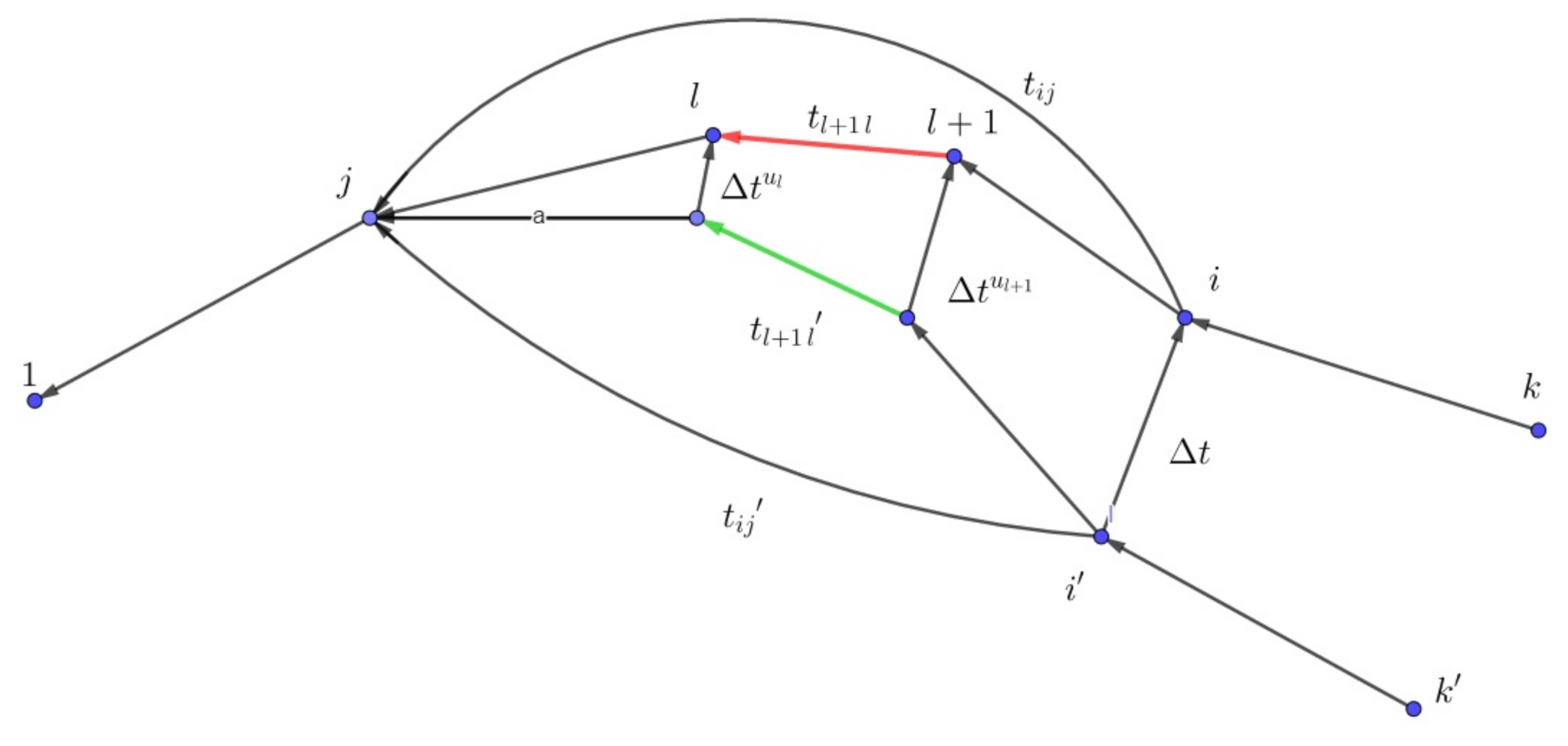
If a match can be substituted by a new match with a smaller overall error, the update should be propagated to all intermediary matches . Some of these matches must have low quality, if such an update can improve the situation. The update involves using the matrix power of a rigid body transformation matrix [31,32] (Ch. 3). Figure 4 depicts a scheme where an additional match is introduced to update all the intermediate incremental matches . The product of transformations in Equation (1) appears as a sequence of arrows from i to j in Figure 4.
The former transformation constructed from incremental matches by Equation ((1)), is updated by Go-ICP to an improved value:
where can be solved by: . Now, each intermediary step can be defined by letting the matrix power of the propagated correction move from 0 to 1:
where approximates the accumulated relative transformation dissimilarity from the frame j to frame l. One can solve the new incremental transformations (depicted in green in Figure 4) by using the definition in Equation (1):
where symbolizes overwriting of the original Go-ICP transformations. There are many possible formulations for the matrix power , which would demand a more theoretic presentation; however, in this study, we chose an approximation, where is the sum of the RMSE match errors of matches , with a scaling to :
The actual matching process builds the resulting tree map to the co-ordinates of the first frame. This is why we actually used the transformations as the interpolant and , where , as the extrapolant of the tail part.
A simplistic strategy to apply corrections is to use indices i and j chosen from a lattice spaced at a 30-frame interval, with limitation . If the match computed by Go-ICP has a better matching error, e, than that of the original (produced by the chain rule of Equation (1)) and the outlier ratio , then an update occurs with the necessary propagation explained earlier.
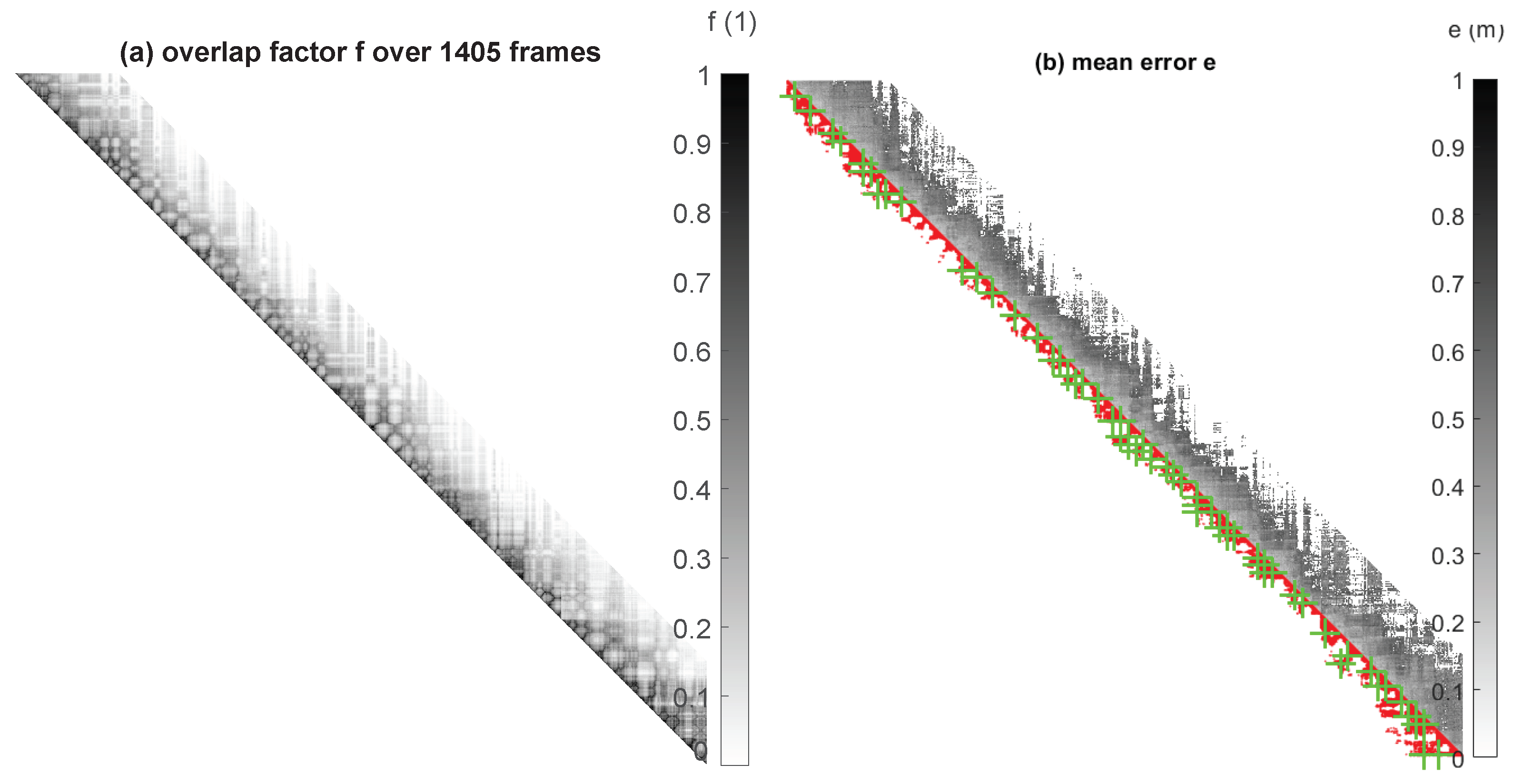
Detail (b) of Figure 5 depicts the extra matches by green crosses. The red zone below the diagonal is the area, where such a large step would be advantageous to make. The grey area shows the mean matching error of the match among point pairs which do not involve outliers. The detail (a) shows the overlap f, which is an observed equivalent of the minimum overlap [33]—also known as the inlier ratio—a commonly used ICP method parameter. Application of the corrections defined by Equation (3) reduces pairwise matching errors, causing the grey stripe of detail (b) to become lighter. The pairwise overlaps do not change much, unless an occasional drastic angular error is corrected.
The selected 4% extra Go-ICP evaluations decrease the noise in the resulting tree map by approximately 38%. The map tree noise is measured by the mean radius of alpha shape clusters [34] of the resulting tree map. The alpha radius m was used to define the alpha shapes. The implementation used was the alphashape.m function [34] in Matlab [35].
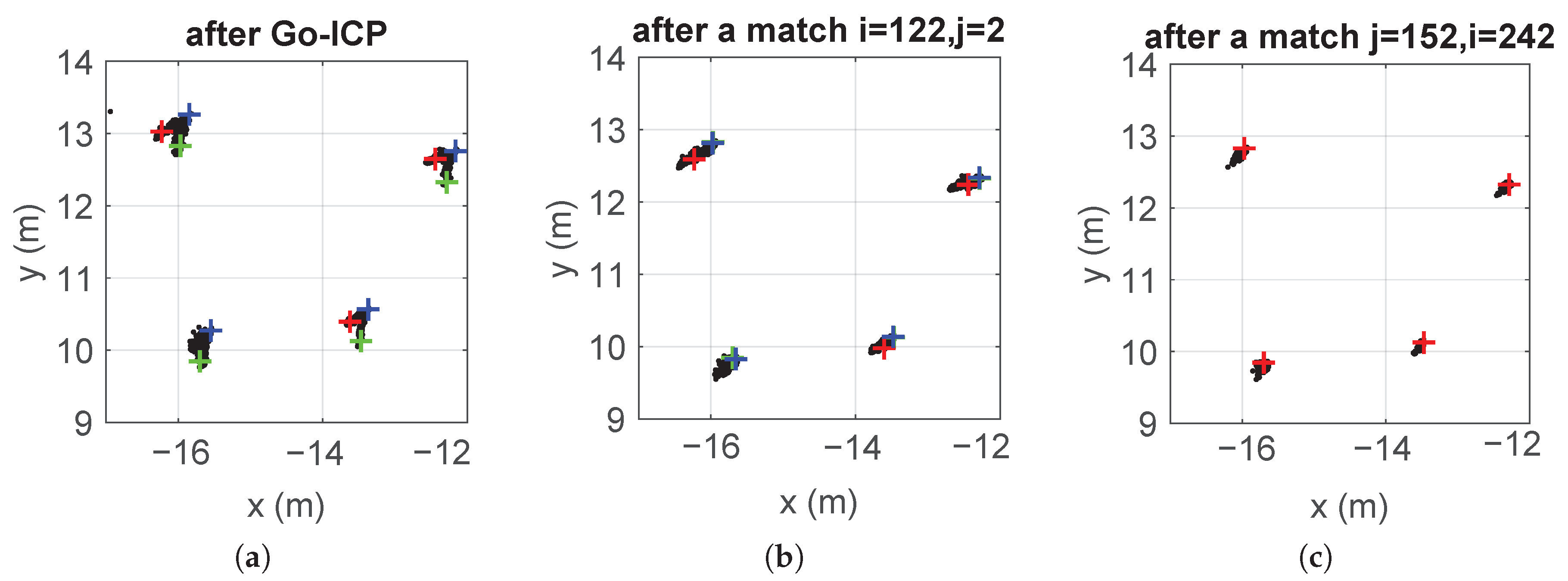
A detail of the tree map is shown in Figure 6. Three frames (red, blue, and green crosses) participated in detecting four trees in detail in (a). A corrective match aligned the green frame to the blue one in detail (b) and, then, the red frame is aligned to the blue one. Notice that both additional alignments propagate to most of the other frames in between the correction pair, causing the error stripe in detail (b) of Figure 5 to become lighter.
The parameters described above (i.e., the search grid and the update condition) were chosen ad hoc, as substitutes for a more controlled algorithm in future work.
The final step was to find alpha shapes of the tree stem clusters for the final map of tree stem segment centers and associate a tree stem center to each alpha shape center. The alpha radius m was the same as used for the tree map noise level evaluation.
Matching the odometry path to the GNSS path: The odometric path and the GNSS path are asynchronous signals. The GNSS location has a z component available but, as mentioned in [36], the elevation error is typically 1.5 times the horizontal error and, so, it was ignored.
The path C was fitted to the path G as a whole, using one single 2D rigid body transformation , where the parameter is for the horizontal rotation and q is a horizontal translation, both subject to minimization processes. By introducing as the nearest point in a point set B to a point q, one can define a symmetric smallest squared projection distance fit with the transformation arguments as:
where the set follows from C by application of a rigid body transformation t, where only the horizontal components of the odometric path C are accessed. The resulting tree map is in global co-ordinates.
2.4. Smooth Deformation for Consistency Checks
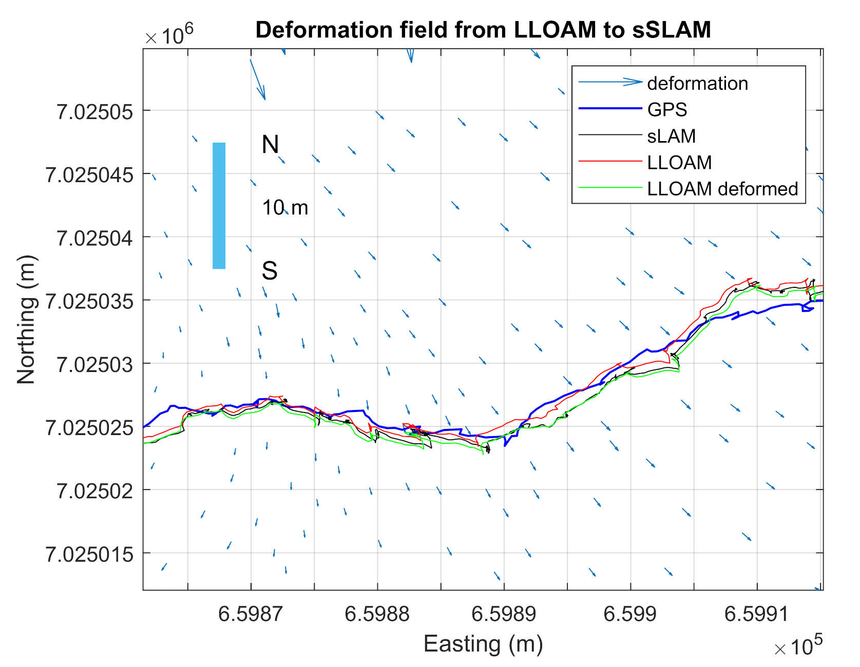
The sSLAM and LLOAM tree maps S and L differ somewhat and it would be interesting to be able to transform smoothly between them, in order to see if some combination would prove to be better, in terms of some performance metrics. A low-pass graph filter [37] of the form
is a graph version of a discrete Laplace operator (applied twice), which was used to interpolate the match difference vector field
where is the assembly matrix of difference vectors , D is the diagonal matrix with degrees of nodes (number of connecting edges), A is the adjacency matrix of the Delaunay triangulation, and is the nearest point to a point . A similar definition can be produced for the PC S by switching the two point sets (L and S) in the definitions. The vector field on L towards S can be depicted as and the one on S towards L as . The interpolated vector field is depicted by blue arrows in Figure 7, at the same scale as the rest of the Figure. The GNSS path is shown in blue, the sSLAM odomatric path is in black, the LLOAM path in red, and the deformed LLOAM in green.
One can smooth by either vector field. A combined PC has and :
where intermediate states (e.g., ) produce close duplicates, one of which has to be eliminated (e.g., when they get closer than 0.6 m from each other). Notice that and are linearly independent, as the nearest neighbors are not symmetric: There exist and , such that , but . There are potential symmetric NN methods (see, e.g., [38]) but, as the smooth adaptation between PCs is used only for verification purposes, the usual NN was used.
3. Results
Consistency checks were made using the deformation fields defined in Section 2.4. Figure 7 shows a section of strip road 3, where the harvester moved from left to right while turning towards the left. This detail shows a systematic difference between sSLAM and LLOAM: Trees detected by sSLAM were systematically further away from the center of the strip road circumference. This phenomenon was small, in the scale of the full strip road, with a relatively balanced amount of arcs to the left and right, however.
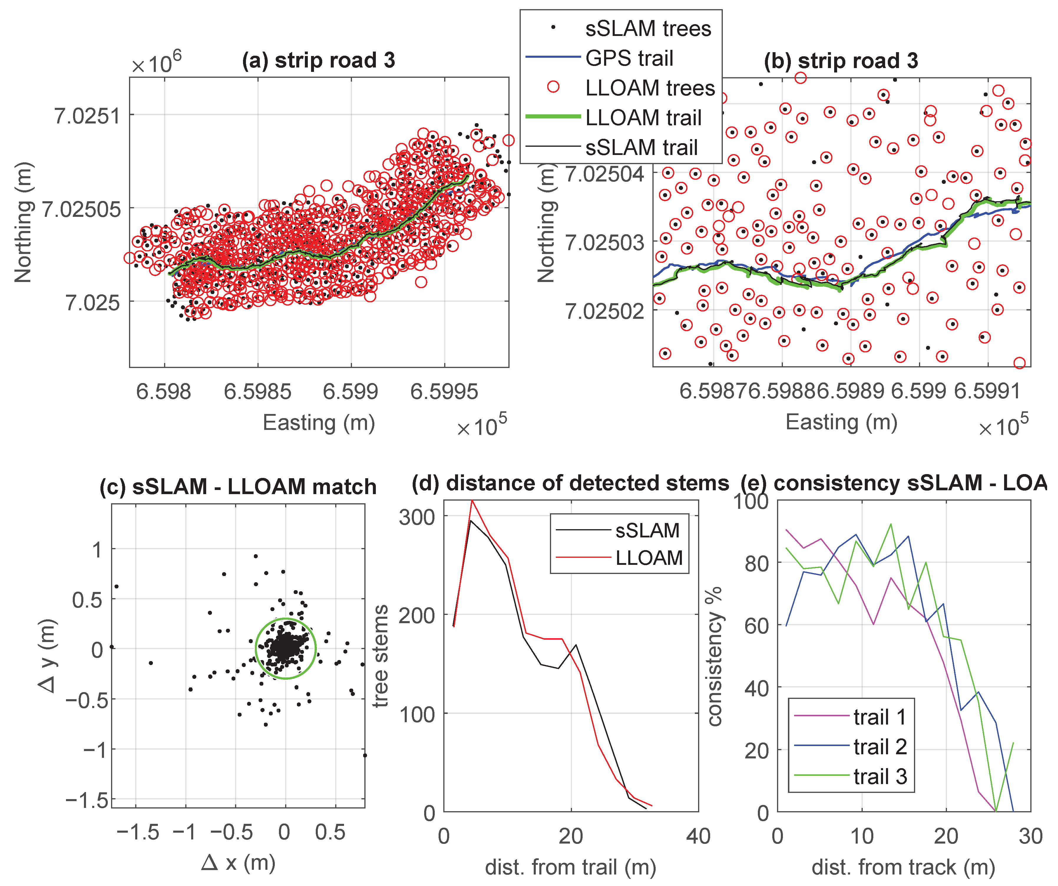
In many metrics, the best weighting of favored sSLAM. One indicator is the placement accuracy, compared to the GNSS location. The latter comprises a large unknown error, but was the only large-scale reference available. Another was the mean PC self-consistency when sample sets were from 50 m long slices of adjacent strip roads. Consistency was measured with the mean match error of the Go-ICP method. Smoothing was done by Equation (7), setting S and L to PCs from different strip roads, the interpolation coefficient to , and the pairing tolerance as 0.3 m. Figure 8 shows how both methods lost some registration accuracy at 15 m.
In both cases, the indicator fell monotonically towards S. The best odometry error value was . This means that the result could not be improved much by mixing both methods. Therefore, numerical indicators were included separately for both methods.
The consistency can be defined as the ratio of matches to the average of the number of points in the two clouds:
The consistency is best illustrated by the tree map (details (a) and (b) in Figure 8). The two methods had rather good agreement to 20 m distance from the strip road, from which point the performance dropped quickly, as can be seen from detail (d) of Figure 8. Detail (c) shows the distances of the detected trees. As one can see, the detection rate decreased almost linearly with the distance and the zone of the nearest 5 m had only two-thirds of the maximum density. The possible reasons for this are discussed in Section 4.
The sSLAM tree map S (black dots) and the deformed PC (red circles) are shown in detail (a) of Figure 8. The deformed tree map was used to make the match logically sound. Detail (c) shows the scatter pattern with a chosen match limit of 0.3 m (green circle). The match limit allows for the association of separate tree stem occurrences from different frames to one tree stem (e.g., for DBM registration). Both methods seemed to be equally good in detecting trees over the considered distance, as shown in the details (d) and (e). The distance in question was perpendicular from the strip road. As seen in Figure 1, strip road 1 had the disadvantage of coming closest to a nearby road, which reduced the detection performance of both methods on that strip road. Both methods had 80% consistency to 15 m distance, which is on the same level as the methods have internally, when judging the overlapping part of the PCs.
The difference, e, between maps L and S was m. This seems large and was not random, as can be seen in Figure 7. Importantly, both methods had consistent detection and this difference did not cause systematic angular deviation, nor odometric dilatation.
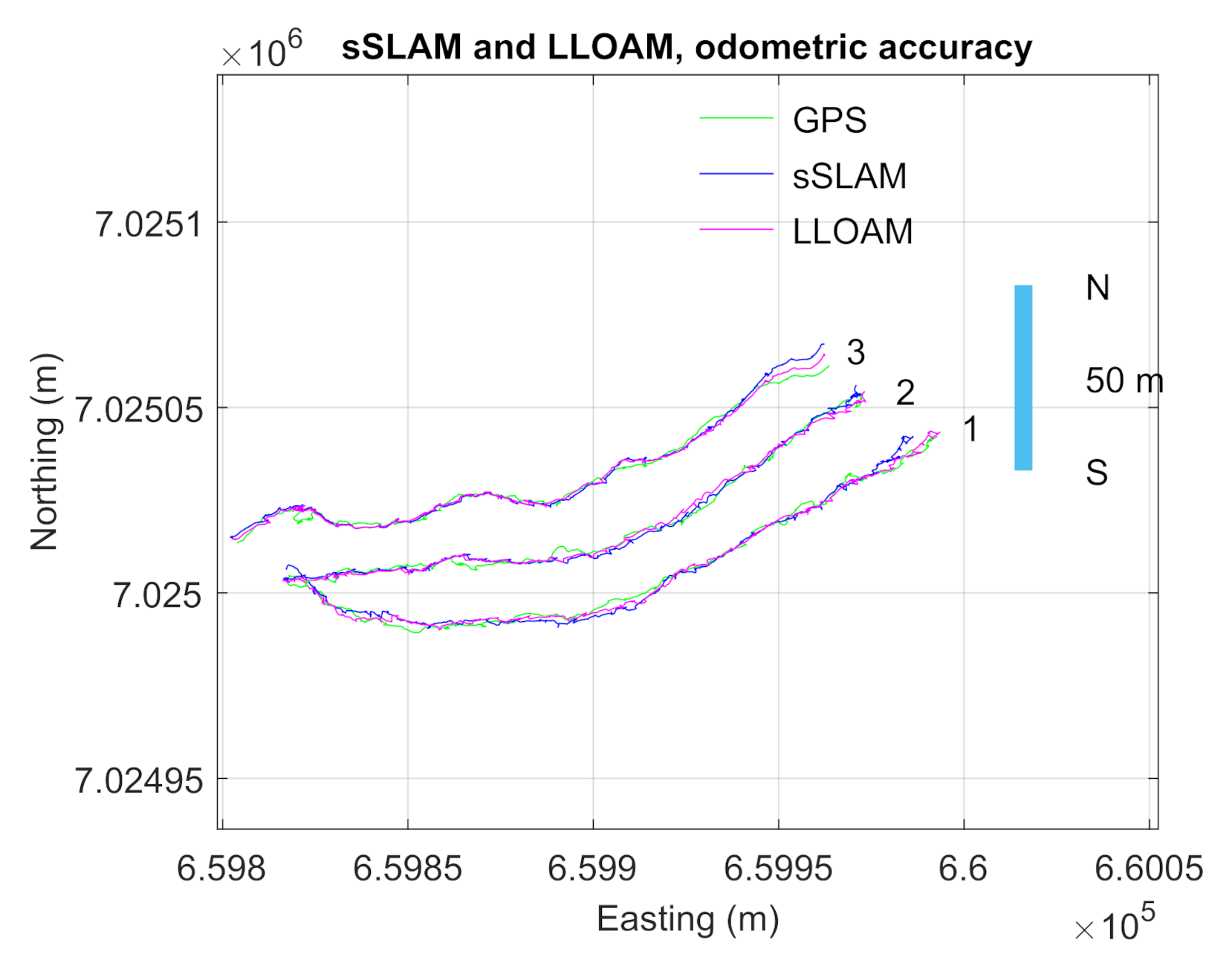
The approximately 0.5 m per 100 m perpendicular odometric error (root mean square error, RMSE) to GNSS location was measured for both methods. See Figure 9, where sSLAM and LLOAM are matched to the GNSS signal.
Table 1 summarizes our various numerical comparisons. The PC size was drastically smaller when using sSLAM. LLOAm classified points to ground hits and edge points, where the edge points were rather close to tree stem hit points. Therefore, the LLOAM cloud had only 1400 hits per tree on average. The GNSS parallel error was measured only for strip road 3, the shape of which allowed for piecewise RMSE matching of odometric paths in 30 m West–East pieces. sSLAM proved to not be as accurate as LLOAM in vertical orientation, compared to DEM. This is partly because the sSLAM end-product is a set of vertical segments corresponding to tree stem center lines, where the lowest point of the visible part of the stem is often hidden by foliage when trees are further away from the scanner.
sSLAM had slightly better horizontal accuracy and LLOAM had better vertical accuracy. Its vertical accuracy results from the ground model detection, which was integrated into the method. Both methods obtained good support from the DEM model, when it was available, to force PCs to the DEM surface. The forcing was implemented by leveraging the lower ends of tree stem segments to the DEM surface (sSLAM) or matching the ground-registered points to the DEM surface (LLOAM). Both matches were formulated by rigid body least squares fitting over the whole length of the strip road, to give an easy reference evaluation.
The mapping range was judged from Figure 8. Both methods fared equally well.
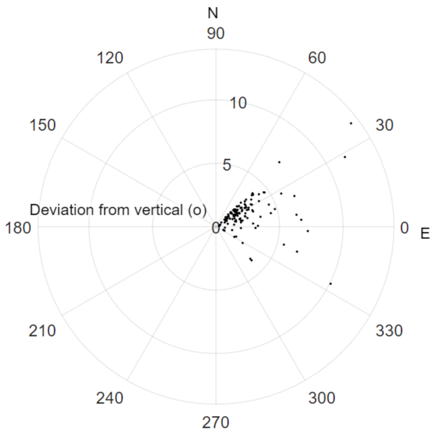
The vertical angular noise was measured from the produced tree stem segments of sSLAM. An ideal result would be to have all registrations in all frames pointing exactly the same way. The s.t.d. of the orientation angle from the mean orientation was measured. Figure 10 depicts the distribution of the detected deviation from the vertical orientation of all trees (approximately 580 trees) along strip road 2. This helps to illustrate the concept of the angular error of an individual tree stem over different frames. Angular error was estimated by measuring the MSE between stem segments of individual frames and the final map depicted in Figure 10. The mean deviation of 2.5 degrees (o) from the vertical seemed to be along the dominant wind direction.
4. Discussion
Our aim was to study the feasibility of sparse PC odometry and mapping. A sparse PC has the advantage of small size; however, there is a certain lack of suitable SLAM methods for such PCs. A dense SLAM has the disadvantage of storing a large passive PC before the final map can be produced. The work cycle of a harvester with a rotating cabin includes large view swings, in which there may be near-perfect repetition of an old view. The effect of swinging is clearly visible, in Figure 5, as repetitive patterns in the match overlap and match error plots. A full-scan method either has to have excellent accuracy or should have access to the data history; sometimes over intervals of two minutes. The proposed alternative has a much lighter memory load, in this respect.
The sSLAM method had a bias, centering the stem segments towards the scanner, as shown in Figure 11. This effect was systematical and neutralized only, if the strip road had similar surroundings on both sides. A similar effect occurred with LLOAM, but to a lesser extent. The strip roads had trees everywhere around, except in the right end of the area (see Figure 9), where sSLAM deviated from the consensus of GNSS and LLOAM. Elsewhere, the consensus of LLOAM and sSLAM seemed more reliable than GNSS which, at times, experienced an escape period during a weak satellite constellation or exceptional tree coverage. One can conclude that a coupled DBH estimate, as an additional and independent process, would be needed if sSLAM were to be used on a site where the harvester is constantly facing one open side.
In separate experiments, we noticed that the deformation between sSLAM and LLOAM maps depicted in Figure 7 disappeared when the LLOAM tree map was formed using 50 m windows, instead of the full 170–190 m strip road window. Our arrangement produced a pessimistic view, as a practical arrangement would require a restricted active window with less discrepancy between the two methods.
The test site was rather flat terrain and the branching height was high (varying between 3 and 6 m), making the site a seemingly easy target. The tree stem diameter varied between 8 and 25 cm (mean 18 cm), which made adjacent tree stem hits on the same channel rare after a distance of 15 m. Furthermore, the continuous work cycle with constant swinging of the horizontal orientation was a new type of source of inaccuracy not met in the existing research.
Odometric errors of 0.2 m per 50 m and 0.5 mper 100 m were observed. These are quite tolerable errors (again shown by both methods). Judging from Figure 9, the GNSS location also had some error, with occasional bursts exceeding 4 m from the consensus of two SLAM methods. This means more accurate environmental markers in global co-ordinates would be needed, in order to assess the odometric accuracy better. The best earlier result was 0.1 m per 100 m drift [11], but this result was obtained using a more dense point cloud, along with the fusion of IMU, GNSS, and SLAM, which we have not yet accomplished.
Tree stem segment center points (marked red in the Figure 11) formed only approximately 1% of the original raw LiDAR data, in this case. Two limiting conditions for the methodology proposed can be concluded: The presence of young trees and the presence of large trees. The former reduced the stem hits, due to their slender stems and prominent branches, and scan range, due to obstruction by foliage. In such environments, a projective PC density method, such as that of [39], could be used. The other environmental limit was thick, old trees, which obstructed further stems, forcing the SLAM accuracy to depend on the closer tree stems. In this kind of environment, the LLOAM method may be the best. The large diameters of the close trees require the integration of DBH registration in the SLAM process. Our intuition is that the method proposed fits in a wide variety of the environments in between these two extremities.
Figure 8, detail (d), shows a drop in detection rate near the path. The reasons for this are twofold: (1) Processing of the felled tree interfered with the SLAM process. This could be countered by careful placing of the laser scanner, although potential for damage dictates its placement for long forest operations. A movie about the SLAM process is available in the samples, which shows that the obstruction is mostly asymmetric and depends on the ’handedness’ of the harvester operator; (2) The harvester followed the strip roads of the first thinning. One can detect a faint outline of the yet-untouched strip road 4 below strip road 3 in detail (a) of Figure 8. This site has economic value and it was mandatory for the harvester to repeat the former movement pattern.
The tree stem segmentation was tested using several other approaches mentioned in Section 1.1. One inspected possibility was the usage of seven generic local PC descriptors, listed in [40]. More features, such as one-dimensionality and vertical stacking, can be defined either for a number of closest points or for a local space partition. Of the tested methods, the proposed method, the voxel voting method of [13], and the combination of them seem promising for the potential application-specific integrated circuit (ASIC) implementation. The actual numerical comparison of all these stem detection methodologies requires more forest types and was, thus, excluded from this study.
NN methods are appealing, due to their conceptual simplicity—after the neural layer definition and training data management have been carried out. PointNet [41] is a DL system which directly consumes PCs and has both quality and computational speed equivalent to that of the existing state-of-the-art systems. NN methods use the supervised learning scheme and, so, gathering a massive volume of positive and negative examples from every possible environment is a key obstacle to their use. PointNet was used as the basic backbone in the study [42], where a semantic-assisted approach was used, which could be adapted to tree stem detection. The tree stem detection method presented in this article could serve as a pre-classifier in the training process for most of the existing NN approaches.
As several new approaches have been introduced (e.g., stem segmentation, reduction of tree map noise by matrix power interpolation), we did not unfold the realms of geopositioning, SLAM, and DEM surface sensor fusion.
5. Conclusions
This work was concerned with testing the quality of a SLAM process in the setting of a practical forestry operation, where no closed loops were available. The physical movement of the harvester was also dictated by the constraints of the boom, while the harvester carried out actual logging operations. The work cycle of the harvester required occasional reversing and the pivoted cabin experienced almost continuous horizontal swinging. This places heavy requirements on the SLAM process.
A comparable accuracy to a current standard SLAM method (LeGO-LOAM, shortened to LLOAM in this text) was demonstrated. The achieved perpendicular accuracy of 0.41 m per 100 m (this being the largest observed deviation along the 500 m of the strip roads) can be considered adequate for constructing complete tree maps with tree locations and DBH; however, the DBH requires local iteration. The methods agree in 80% of registrations to 15 m perpendicular distance from the strip road.
The improvement of SLAM by matrix power interpolation seems to be a simple method to reduce the SLAM error, resulting from non-focal observations of tree stem segments. This interpolation trick is generic and can be applied to all other SLAM methods, which have cheap match error computation. There are more possible formulations for the problem, however. One is the use of a regression technique over rigid body transformations [43], while another represents Gaussian processes over the same domain [44], which could be used, in an iterative manner, to substitute for the power method.
The next steps of our research will be: (1) To optimize the number of correction steps. The correction uses a hard-coded lattice of additional matches now. (2) To improve Go-ICP and adapt it better to approximately uniformly distributed trees. This would include using ICP when it is proven to be safe.
The vertical accuracy of SLAM had an effect in branch height detection and, indirectly, to species registration. As the proposed sSLAM method had a max vertical error 0.9 m, it likely requires some sort of post-processing for the foliage PCs of individual trees. These aspects will be tested in future studies.
It is also possible to record the positions of felled and processed tree stems directly from the harvester processing head (see, e.g., [45,46]) and record them, relative to the tree stems of the remaining trees. This reference information has a location error of less than 0.5 m [46], which could then be used in the collection phase, which can rely on the produced tree map [3]. The improvement gained from the use of an inertial measurement unit (IMU) signal remains to be tested, as well. This provides a possible addition to the intended system, which further demands the sleek and effortless performance of the SLAM and tree map pipeline.
Most of the proposals rely on LiDAR scanning. However, commercial utilization requires resilience under rain, snow cover, and night. This may not be possible without sensor fusion and several sensor types. A longer effort would be to find a combination of methodologies and processing steps which, together, are reliable over a wide range of forest environments and can support a wide enough range of forest operations. For this, the proposed modular approach is appealing, as it allows for continuous experimentation and the improvement of the submodules.
Supplementary Materials
The following are available at https://seafile.utu.fi/d/6dacb1ec9b1c4e5685ef/: Tree stem registration based on Delaunay neighborhoods.
Author Contributions
Conceptualization, P.N. and T.M.; methodology, P.N.; software, Q.L.; validation, P.N., K.R., Q.L. and T.M.; formal analysis, P.N.; investigation, P.N.; resources, J.H.; data curation, T.M. and K.R.; writing—original draft preparation, P.N.; writing—review and editing, P.N.; visualization, P.N., and T.M.; supervision, T.W. and J.H.; project administration, T.M., J.H.; funding acquisition, J.H. All authors have read and agreed to the published version of the manuscript.
Funding
This research was funded by Business Finland grant number 26004155.
Acknowledgments
The data from the study area were gathered in co-operation with Stora Enso Wood Suply Finland, Metsäteho Oy and Aalto University. The data collection was done under the EFFORTE, Efficient forestry for sustainable and cost-competitive bio-based industry (2016–2019) in WP3—Big data databases and applications.
Conflicts of Interest
The authors declare no conflict of interest.
References
- Benjamin, J.G.; Seymour, R.S.; Meacham, E.; Wilson, J. Impact of Whole-Tree and Cut-to-Length Harvesting on Postharvest Condition and Logging Costs for Early Commercial Thinning in Maine. North. J. Appl. For. 2013, 30, 149–155. Available online: http://xxx.lanl.gov/abs/https://0-academic-oup-com.brum.beds.ac.uk/njaf/article-pdf/30/4/149/23416324/2384.pdf (accessed on 25 November 2020). [CrossRef]
- Szewczyk, G.; Spinelli, R.; Magagnotti, N.; Tylek, P.; Sowa, J.M.; Rudy, P.; Gaj-Gielarowiec, D. The mental workload of harvester operators working in steep terrain conditions. Silva Fenn 2020, 54, 10355. [Google Scholar] [CrossRef]
- Li, Q.; Nevalainen, P.; Peña Queralta, J.; Heikkonen, J.; Westerlund, T. Localization in Unstructured Environments: Towards Autonomous Robots in Forests with Delaunay Triangulation. arXiv, 2020; arXiv:2005.05662. [Google Scholar]
- Pierzchała, M.; Giguére, P.; Astrup, R. Mapping forests using an unmanned ground vehicle with 3D LiDAR and graph-SLAM. Comput. Electron. Agric. 2018, 145, 217–225. [Google Scholar] [CrossRef]
- Nevalainen, O.; Honkavaara, E.; Tuominen, S.; Viljanen, N.; Hakala, T.; Yu, X.; Hyyppä, J.; Saari, H.; Pölönen, I.; Imai, N.; et al. Individual Tree Detection and Classification with UAV-Based Photogrammetric Point Clouds and Hyperspectral Imaging. Remote Sens. 2017, 9, 185. [Google Scholar] [CrossRef] [Green Version]
- Zhao, G.; Shao, G.; Reynolds, K.; Wimberly, M.; Warner, T.; Moser, J.; Rennolls, K.; Magnussen, S.; Köhl, M.; Anderson, H.E.; et al. Digital Forestry: A White Paper. J. For. 2005, 103, 47–50. [Google Scholar]
- Cadena, C.; Carlone, L.; Carrillo, H.; Latif, Y.; Scaramuzza, D.; Neira, J.; Reid, I.; Leonard, J.J. Past, Present, and Future of Simultaneous Localization and Mapping: Toward the Robust-Perception Age. Trans. Rob. 2016, 32, 1309–1332. [Google Scholar] [CrossRef] [Green Version]
- Liang, X.; Hyyppä, J.; Kaartinen, H.; Lehtomäki, M.; Pyörälä, J.; Pfeifer, N.; Holopainen, M.; Brolly, G.; Francesco, P.; Hackenberg, J.; et al. International benchmarking of terrestrial laser scanning approaches for forest inventories. ISPRS J. Photogramm. Remote Sens. 2018, 144, 137–179. [Google Scholar] [CrossRef]
- Sprickerhof, J.; Nuchter, A.; Lingemann, K.; Hertzberg, J. An explicit loop closing technique for 6d SLAM. In Proceedings of the 4th European Conference on Mobile Robots, ECMR-09, Mlini/Dubrovnik, Croatia, 23–25 September 2009; pp. 229–234. [Google Scholar]
- de Conto, T. Performance of tree stem isolation algorithms for terrestrial laser scanning point clouds. In Examensarbete / SLU; Institutionen För Sydsvensk Skogsvetenskap: Alnarp, Sweden, 2016; Volume 262. [Google Scholar]
- Tang, J.; Chen, Y.; Kukko, A.; Kaartinen, H.; Jaakkola, A.; Khoramshahi, E.; Hakala, T.; Hyyppä, J.; Holopainen, M.; Hyyppä, H. SLAM aided Stem Mapping for Forest Inventory with Small-footprint Mobile LiDAR. Forests 2015, 6, 4588–4606. [Google Scholar] [CrossRef] [Green Version]
- Hosoi, F.; Nakai, Y.; Omasa, K. Voxel tree modeling for estimating leaf area density and woody material volume using 3-D LIDAR data. Isprs Ann. Photogramm. Remote. Sens. Spat. Inf. Sci. 2013, II-5/W2, 115–120. [Google Scholar] [CrossRef] [Green Version]
- Heinzel, J.; Huber, M.O. Detecting Tree Stems from Volumetric TLS Data in Forest Environments with Rich Understory. Remote Sens. 2017, 9, 9. [Google Scholar] [CrossRef] [Green Version]
- Guan, H.; Yu, Y.; Yan, W.; Li, D.; Li, J. 3D-Cnn Based Tree species classification using mobile lidar data. ISPRS Int. Arch. Photogramm. Remote. Sens. Spat. Inf. Sci. 2019, XLII-2/W13, 989–993. [Google Scholar] [CrossRef] [Green Version]
- Zhang, W.; Wan, P.; Wang, T.; Cai, S.; Chen, Y.; Jin, X.; Yan, G. A Novel Approach for the Detection of Standing Tree Stems from Plot-Level Terrestrial Laser Scanning Data. Remote Sens. 2019, 11, 211. [Google Scholar] [CrossRef] [Green Version]
- Arachchige, N.H. Automatic tree stem detection of a geometric feature based approach for MLS point clouds. ISPRS Ann. Photogramm. Remote. Sens. Spat. Inf. Sci. 2013, II-5/W2, 109–114. [Google Scholar] [CrossRef] [Green Version]
- Wang, J.; Chen, X.; Cao, L.; An, F.; Chen, B.; Xue, L.; Yun, T. Individual Rubber Tree Segmentation Based on Ground-Based LiDAR Data and Faster R-CNN of Deep Learning. Forests 2019, 10, 793. [Google Scholar] [CrossRef] [Green Version]
- Miettinen, M.; Öhman, M.; Visala, A.; Forsman, P. Simultaneous localization and mapping for forest harvesters. In Proceedings of the IEEE International Conference on Robotics and Automation, Roma, Italy, 10–14 April 2007; pp. 517–522. [Google Scholar]
- Zhang, J.; Singh, S. LOAM: Lidar Odometry and Mapping in Real-time. In Proceedings of the 2014 Robotics: Science and Systems Conference, Berkeley, CA, USA, 13–15 July 2014. [Google Scholar]
- Chen, S.; Nardari, G.; Lee, E.; Qu, C.; Liu, X.; Romero, R.; Kumar, V. SLOAM: Semantic Lidar Odometry and Mapping for Forest Inventory. IEEE Robot. Autom. Lett. 2020, 5. [Google Scholar] [CrossRef] [Green Version]
- Segal, A.; Hähnel, D.; Thrun, S. Generalized-ICP. In Robotics: Science and Systems; Trinkle, J., Matsuoka, Y., Castellanos, J.A., Eds.; The MIT Press: Cambridge, MA, USA, 2009. [Google Scholar]
- Rusu, R.B.; Cousins, S. 3D is here: Point Cloud Library (PCL). In Proceedings of the 2011 IEEE International Conference on Robotics and Automation (ICRA), Shanghai, China, 9–13 May 2011. [Google Scholar]
- Wen, S.; Zhao, Y.; Yuan, X.; Wang, Z.; Zhang, D.; Manfredi, L. Path planning for active SLAM based on deep reinforcement learning under unknown environments. Intell. Serv. Robot. 2020, 13, 263–272. [Google Scholar] [CrossRef]
- Shan, T.; Englot, B. LeGO-LOAM: Lightweight and Ground-Optimized Lidar Odometry and Mapping on Variable Terrain. In Proceedings of the 2018 IEEE/RSJ International Conference on Intelligent Robots and Systems (IROS), Madrid, Spain, 1–5 October 2018; pp. 4758–4765. [Google Scholar] [CrossRef]
- Yang, J.; Li, H.; Campbell, D.; Jia, Y. Go-ICP: A Globally Optimal Solution to 3D ICP Point-Set Registration. IEEE Trans. Pattern Anal. Mach. Intell. 2016, 38, 2241–2254. [Google Scholar] [CrossRef] [Green Version]
- Bello, S.A.; Yu, S.; Wang, C. Review: Deep learning on 3D point clouds. arXiv 2020, arXiv:cs.CV/2001.06280. [Google Scholar] [CrossRef]
- Li, Q.; Chen, S.; Wang, C.; Li, X.; Wen, C.; Cheng, M.; Li, J. LO-Net: Deep Real-Time Lidar Odometry. In Proceedings of the IEEE/CVF Conference on Computer Vision and Pattern Recognition (CVPR), Long Beach, CA, USA, 15–21 June 2019; pp. 8465–8474. [Google Scholar]
- Liang, X.; Kankare, V.; Hyyppä, J.; Wang, Y.; Kukko, A.; Haggrén, H.; Yu, X.; Kaartinen, H.; Jaakkola, A.; Guan, F.; et al. Terrestrial laser scanning in forest inventories. Theme issue ‘State-of-the-art in photogrammetry, remote sensing and spatial information science’. ISPRS J. Photogramm. Remote Sens. 2016, 115, 63–77. [Google Scholar] [CrossRef]
- Kaartinen, H.; Hyyppä, J.; Vastaranta, M.; Kukko, A.; Jaakkola, A.; Yu, X.; Pyörälä, J.; Liang, X.; Liu, J.; Wang, Y.; et al. Accuracy of Kinematic Positioning Using Global Satellite Navigation Systems under Forest Canopies. Forests 2015, 6, 3218–3236. [Google Scholar] [CrossRef]
- Oksanen, J.; Sarjakoski, T. Error Propagation of DEM-Based Surface Derivatives. Comput. Geosci. 2005, 31, 1015–1027. [Google Scholar] [CrossRef]
- Lynch, K.M.; Park, F.C. Modern Robotics: Mechanics, Planning, and Control, 1st ed.; Cambridge University Press: Cambridge, MA, USA, 2017. [Google Scholar]
- Eberly, D. Interpolation of Rigid Motions in 3D. 2017. Available online: https://www.geometrictools.com/Documentation/InterpolationRigidMotions.pdf (accessed on 21 October 2020).
- Chetverikov, D.; Svirko, D.; Stepanov, D.; Krsek, P. The Trimmed Iterative Closest Point algorithm. In Proceedings of the Object Recognition Supported by User Interaction for Service Robots, Quebec City, QC, Canada, 11–15 August 2002; Volume 3, pp. 545–548. [Google Scholar] [CrossRef]
- Akkiraju, N.; Edelsbrunner, H.; Facello, M.; Fu, P.; Mücke, E.P.; Varela, C. Alpha shapes: Definition and software. In Proceedings of the 1st International Computational Geometry Software Workshop (GCG), Minneapolis, MN, USA, 11 September 1995. [Google Scholar]
- The Mathworks, Inc. MATLAB Version 9.8.0.1323502 (R2020a); The Mathworks, Inc.: Natick, MA, USA, 2020. [Google Scholar]
- Pırtı, A. Accuracy Analysis of GPS Positioning Near the Forest Environment. Croat. J. For. Eng. 2008, 29, 189–199. [Google Scholar]
- Stankovic, L.; Dakovic, M.; Sejdic, E. Introduction to Graph Signal Processing. In Vertex-Frequency Analysis of Graph Signals; Stanković, J., Sejdić, E., Eds.; Springer: Cham, Switzerland, 2019; pp. 3–108. [Google Scholar] [CrossRef]
- Nock, R.; Sebban, M.; Jappy, P. A Symmetric Nearest Neighbor Learning Rule. In Advances in Case-Based Reasoning; Blanzieri, E., Portinale, L., Eds.; Springer: Berlin/Heidelberg, Germany, 2000; pp. 222–233. [Google Scholar]
- Sihvo, S.; Virjonen, P.; Nevalainen, P.; Heikkonen, J. Tree detection around forest harvester based on onboard LiDAR measurements. In Proceedings of the 2018 Baltic Geodetic Congress (BGC Geomatics), Olsztyn, Poland, 21–23 June 2018. [Google Scholar] [CrossRef]
- Hillemann, M.; Weinmann, M.; Mueller, M.S.; Jutzi, B. Automatic Extrinsic Self-Calibration of Mobile Mapping Systems Based on Geometric 3D Features. Remote Sens. 2019, 11, 1955. [Google Scholar] [CrossRef] [Green Version]
- Qi, C.R.; Su, H.; Mo, K.; Guibas, L.J. PointNet: Deep Learning on Point Sets for 3D Classification and Segmentation. arXiv 2016, arXiv:1612.00593. [Google Scholar]
- Zaganidis, A.; Sun, K.; Duckett, T.; Cielniak, G. Integrating Deep Semantic Segmentation Into 3-D Point Cloud Registration. IEEE Robot. Autom. Lett. 2018. [Google Scholar] [CrossRef] [Green Version]
- Funatomi, T.; Iiyama, M.; Kakusho, K.; Minoh, M. Regression of 3D rigid transformations on real-valued vectors in closed form. In Proceedings of the 2017 IEEE International Conference on Robotics and Automation (ICRA), Singapore, 30 May–5 June 2017; pp. 6412–6419. [Google Scholar] [CrossRef]
- Lang, M.; Dunkley, O.; Hirche, S. Gaussian process kernels for rotations and 6D rigid body motions. In Proceedings of the 2014 IEEE International Conference on Robotics and Automation (ICRA), Hong Kong, China, 31 May–7 June 2014; pp. 5165–5170. [Google Scholar] [CrossRef] [Green Version]
- Saukkola, A.; Melkas, T.; Riekki, K.; Sirparanta, S.; Peuhkurinen, J.; Holopainen, M.; Hyyppä, J.; Vastaranta, M. Predicting Forest Inventory Attributes Using Airborne Laser Scanning, Aerial Imagery, and Harvester Data. Remote Sens. 2019, 11, 797. [Google Scholar] [CrossRef] [Green Version]
- Lindroos, O.; Ringdahl, O.; La Hera, P.X.; Hohnloser, P.; Hellström, T. Estimating the Position of the Harvester Head–a Key Step towards the Precision Forestry of the Future? Croat. J. For. Eng. 2015, 36, 147–164. [Google Scholar]
Figure 1.
(a) Three strip roads (orange) of the forest harvester at the test site after the thinning process. The strip roads 1–3 are at approximately 20–25 m distance from each other. (b) The test site in Lieksa, Eastern Finland.
Figure 1.
(a) Three strip roads (orange) of the forest harvester at the test site after the thinning process. The strip roads 1–3 are at approximately 20–25 m distance from each other. (b) The test site in Lieksa, Eastern Finland.

Figure 2.
(a) Komatsu Forest 931.1 forest harvester. The LiDAR scanner is attached in the front of the windshield of the cabin (orange circle), giving a 210 view forwards. (b) A close-up of the LiDAR scanner.
Figure 2.
(a) Komatsu Forest 931.1 forest harvester. The LiDAR scanner is attached in the front of the windshield of the cabin (orange circle), giving a 210 view forwards. (b) A close-up of the LiDAR scanner.

Figure 3.
Creating tree maps through the two process paths.

Figure 4.
A suspicious match (red) is improved using a reliable match (black). The local path and the corresponding transformation are updated (green). The total update at the frame i equals and happens in the transformation space. The perceived physical change is the opposite of .
Figure 4.
A suspicious match (red) is improved using a reliable match (black). The local path and the corresponding transformation are updated (green). The total update at the frame i equals and happens in the transformation space. The perceived physical change is the opposite of .

Figure 5.
(a) Overlap f over the range of all pairs of frames. The overlap (black) means that the match covers all tree stems and there are no outliers. (b) The mean match error (grey) over all pairs of frames and over all non-outliers. The error becomes noisy when the overlap falls below and is not displayed. Red indicates pairs with match error m and outlier ratio . Green ’+’ signs indicate the chosen 60 extra matches.

Figure 6.
Two corrective matches done to four trees along strip road 1. (a) Initial raw tree map produced by Go-ICP. (b) The first correction, where a frame (blue) is matched with frame (green cross). (c) The second correction, where a frame is matched with frame (red cross).
Figure 6.
Two corrective matches done to four trees along strip road 1. (a) Initial raw tree map produced by Go-ICP. (b) The first correction, where a frame (blue) is matched with frame (green cross). (c) The second correction, where a frame is matched with frame (red cross).

Figure 7.
The continuous deformation field (blue arrows) from the LLOAM data to the sSLAM data around strip road 3. The deformation field maps the original LLOAM odometry (red line) closer to SLAM (green line), based on the match discrepancy everywhere. The GNSS track is in blue and the sSLAM odometry is in black.

Figure 8.
Top: (a) The tree map produced by sSLAM (black dots) and by deformed LLOAM (red circles). (b) A close-up of (a), matching Figure 7. Below: (c) The scatter image between the nearest LLOAM tree from each sSLAM tree. (d) The distribution of the perpendicular distance of detected trees from the strip road. (e) The consistency between the two methods over perpendicular distance from the strip road.

Figure 9.
Odometric paths of three methods compared. The mean error was approximately 0.8 m between GNSS and the two methods. The disagreement on the right end is caused by a lack of trees in the scanning range.
Figure 9.
Odometric paths of three methods compared. The mean error was approximately 0.8 m between GNSS and the two methods. The disagreement on the right end is caused by a lack of trees in the scanning range.

Figure 10.
Stem segment orientations along strip road 2.

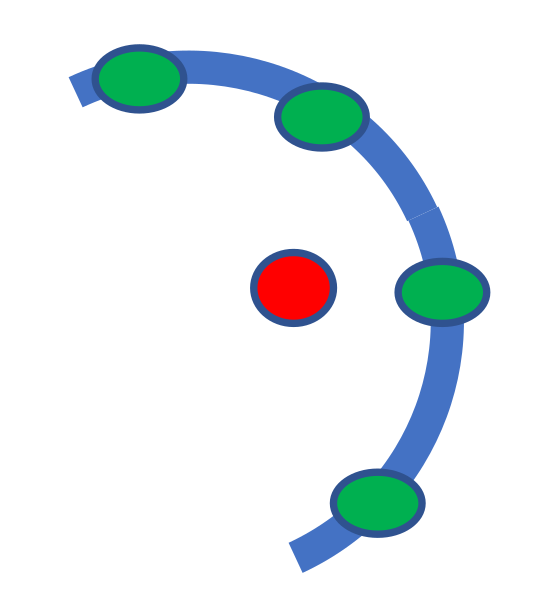
Figure 11.
Tree stem segment (red) aligned by the hit points (green) on the stem surface, where most stems have too few points for the cylinder fit to succeed on a frame-by-frame basis.
Figure 11.
Tree stem segment (red) aligned by the hit points (green) on the stem surface, where most stems have too few points for the cylinder fit to succeed on a frame-by-frame basis.


Table 1.
Odometric accuracy. Units are called over a 100 m distance.
| Measurement | sSLAM | LLOAM |
|---|---|---|
| PC size after stem detection | 450 | 63,000 |
| GNSS parallel error (m) | 0.41 | 0.84 |
| Vertical accuracy (m) | 0.94 | 0.37 |
| Vertical angular noise () | 2.0 | – |
| Mapping range (m) | 20 | 20 |
| Self-consistency (%) | 79 | 75 |
| Self-consistency in parts (%) | 85 | 77 |
Sample Availability: The data presented in this study are openly available in Harvard Dataverse at 10.7910/DVN/IO7PZO. |
Publisher’s Note: MDPI stays neutral with regard to jurisdictional claims in published maps and institutional affiliations. |
© 2020 by the authors. Licensee MDPI, Basel, Switzerland. This article is an open access article distributed under the terms and conditions of the Creative Commons Attribution (CC BY) license (http://creativecommons.org/licenses/by/4.0/).
Share and Cite
MDPI and ACS Style
Nevalainen, P.; Li, Q.; Melkas, T.; Riekki, K.; Westerlund, T.; Heikkonen, J. Navigation and Mapping in Forest Environment Using Sparse Point Clouds. Remote Sens. 2020, 12, 4088. https://0-doi-org.brum.beds.ac.uk/10.3390/rs12244088
AMA Style
Nevalainen P, Li Q, Melkas T, Riekki K, Westerlund T, Heikkonen J. Navigation and Mapping in Forest Environment Using Sparse Point Clouds. Remote Sensing. 2020; 12(24):4088. https://0-doi-org.brum.beds.ac.uk/10.3390/rs12244088
Chicago/Turabian StyleNevalainen, Paavo, Qingqing Li, Timo Melkas, Kirsi Riekki, Tomi Westerlund, and Jukka Heikkonen. 2020. "Navigation and Mapping in Forest Environment Using Sparse Point Clouds" Remote Sensing 12, no. 24: 4088. https://0-doi-org.brum.beds.ac.uk/10.3390/rs12244088
Note that from the first issue of 2016, this journal uses article numbers instead of page numbers. See further details here.