Technical Note

Himawari-8 Aerosol Optical Depth (AOD) Retrieval Using a Deep Neural Network Trained Using AERONET Observations

1
College of Resources and Environmental Science, Ningxia University, Yinchuan 750021, China
2
Geography and Geospatial Sciences, Geospatial Sciences Center of Excellence, South Dakota State University, Brookings, SD 57007, USA
3
State Key Laboratory of Remote Sensing Science, Aerospace Information Research Institute, Chinese Academy of Sciences, Beijing 100101, China
4
Royal Netherlands Meteorological Institute (KNMI), R&D Satellite Observations, 3730 AE De Bilt, The Netherlands
5
Department of Geography and Resource Management, Institute of Space and Earth Information Science, The Chinese University of Hong Kong, Shatin, N.T., Hong Kong, China
*
Author to whom correspondence should be addressed.
Remote Sens. 2020, 12(24), 4125; https://0-doi-org.brum.beds.ac.uk/10.3390/rs12244125
Submission received: 19 November 2020 / Revised: 13 December 2020 / Accepted: 16 December 2020 / Published: 17 December 2020
(This article belongs to the Special Issue Active and Passive Remote Sensing of Aerosols and Clouds)

Abstract

:
Spectral aerosol optical depth (AOD) estimation from satellite-measured top of atmosphere (TOA) reflectances is challenging because of the complicated TOA-AOD relationship and a nexus of land surface and atmospheric state variations. This task is usually undertaken using a physical model to provide a first estimate of the TOA reflectances which are then optimized by comparison with the satellite data. Recently developed deep neural network (DNN) models provide a powerful tool to represent the complicated relationship statistically. This study presents a methodology based on DNN to estimate AOD using Himawari-8 Advanced Himawari Imager (AHI) TOA observations. A year (2017) of AHI TOA observations over the Himawari-8 full disk collocated in space and time with Aerosol Robotic Network (AERONET) AOD data were used to derive a total of 14,154 training and validation samples. The TOA reflectance in all six AHI solar bands, three TOA reflectance ratios derived based on the dark-target assumptions, sun-sensor geometry, and auxiliary data are used as predictors to estimate AOD at 500 nm. The DNN AOD is validated by separating training and validation samples using random k-fold cross-validation and using AERONET site-specific leave-one-station-out validation, and is compared with a random forest regression estimator and Japan Meteorological Agency (JMA) AOD. The DNN AOD shows high accuracy: (1) RMSE = 0.094, R2 = 0.915 for k-fold cross-validation, and (2) RMSE = 0.172, R2 = 0.730 for leave-one-station-out validation. The k-fold cross-validation overestimates the DNN accuracy as the training and validation samples may come from the same AHI pixel location. The leave-one-station-out validation reflects the accuracy for large-area applications where there are no training samples for the pixel location to be estimated. The DNN AOD has better accuracy than the random forest AOD and JMA AOD. In addition, the contribution of the dark-target derived TOA ratio predictors is examined and confirmed, and the sensitivity to the DNN structure is discussed.

Graphical Abstract

1. Introduction

Aerosols play an important role in the Earth’s radiation balance, hydrological cycle, and biogeochemical cycles [1]. Spectral aerosol optical depth (AOD), defined as the extinction of solar radiation due to aerosols, as function of wavelength and integrated over the whole atmospheric column, is one of the principal parameters retrieved from satellite observations. Many different AOD retrieval algorithms have been developed and most of them use radiative transfer models (RTMs) to develop relations between the observed top-of-atmosphere (TOA) reflectance and AOD and assume prior knowledge of the surface reflectance and the aerosol type [2,3]. The RTMs calculate the scattering and absorption of solar radiation by atmospheric molecules and aerosols, which is time consuming and, to save computer time, usually look up tables (LUTs) are created providing RTM results for discrete values of the deciding input parameters such as the angles describing the observation geometry, aerosol models, and discrete values of the AOD. Data from a wide variety of instruments on board different satellite platforms have been used for AOD retrieval. Apart from relying on RTMs, each sensor algorithm may be different and designed specifically for sensor characteristics [4], e.g., spectral band configuration [5,6], multiple view capability [7,8], and polarization [9,10].
Most satellite AOD products are derived from polar orbit satellite sensors. Recently launched new generation geostationary sensors provide bands suitable for AOD retrieval with high revisit times (every 0.5–15 min). The Advanced Himawari Imager (AHI) on board the Himawari-8 satellite, launched in 2014, is such a sensor. The current AHI aerosol product [11] retrieves AOD using a deep-blue (DB)-type method. The DB method, using a pre-calculated static surface reflectance, was originally developed for bright surface [12] and the enhanced DB algorithm can be used over all land types [13,14,15]. In addition, other classical RTM-based AOD retrieval methods were applied to AHI AOD retrieval, such as dark-target (DT) [16,17] and multiangle implementation of atmospheric correction (MAIAC) [18,19]. DT [5] assumes fixed ratios between the visible and 2.1 μm shortwave infrared band surface reflectances. MAIAC jointly retrieves the AOD and the surface anisotropic reflectance using multiple MODIS observations [20,21]. It was originally developed for the MODIS sensor and NASA plans to implement the algorithm for the geostationary satellites including Himawari in the GeoNEX project [18].
In this study, we explore the use of data-driven machine learning methods to derive AOD from AHI observations to investigate whether the data-driven method could achieve at least a similar level of accuracy as the RTM-based AOD retrieval. It is motivated by the recent development of deep neural network (DNN) algorithms [22] providing capability to model complicated relationships and by Aerosol Robotic Network (AERONET) observations providing training samples [23]. A few studies have been undertaken using a shallow artificial neural network (ANN) to directly estimate AOD from satellite TOA measurements, but these were applied to a limited study area [24,25,26,27]. Machine learning methods have also been applied to correct measurement errors in the RTM-based AOD retrieval [28,29,30], to build surface reflectance relationships in the DT algorithm [31], and to estimate AOD with surface reflectance as predictors [32]. To our best knowledge, there has been no publication related to the retrieval of aerosol properties directly using AHI TOA data based on deep neural networks.
The DNN predictors include TOA reflectance, TOA reflectance ratios derived from the DT assumption, sun-sensor geometry, and auxiliary data that are used for the RTM-based AOD retrieval so that the RTM and DNN-based AOD retrieval can be fairly compared (i.e., using the same input information). To train and validate the DNN, a dataset is created consisting of one year (2017) of AHI TOA reflectances collocated in space and time with AERONET AOD over the Himawari-8 full disk. The DNN is trained using state-of-the-art techniques to achieve its full capability. The DNN is compared to an established random forest regression algorithm that has been extensively used for estimation of atmospheric components using remote sensing data [33,34,35,36]. The paper is structured as follows. The Himawari-8, AERONET, and auxiliary data are introduced in Section 2 and the methodology is described in Section 3. The results are presented in Section 4 and the sensitivity to DNN structure and the contributions of TOA reflectance ratio predictors are discussed in Section 5. Conclusions are summarized in Section 6.

2. Data

2.1. Himawari-8 TOA Reflectance and AOD, and Auxiliary Data

Himawari-8 is a geostationary satellite launched by the Japan Meteorological Agency (JMA) in 2014 and positioned at 140.7°E, with a spatial coverage of 150° by 150°. The AHI on board Himawari-8 provides multi-spectral observations every 10 min. The AHI images include six bands in the solar spectrum, including three visible and three near-infrared bands with different spatial resolutions from 0.5 to 2 km at the sub-satellite point. The relative radiometric uncertainty of the AHI measurements is <3% for bands 1–4 and ~5% for bands 5–6 [37,38]. The AHI data were processed into different levels. The Himawari L1 data (Himawari L1 Gridded data) distributed by JMA is generated from the Himawari standard data with re-sampling to equal latitude-longitude grids, which have a spatial coverage of 120° by 120°, centered at 0°N, 140°E. The Himawari L1 data provide the TOA reflectances in all the six reflective bands (Table 1) resampled to 2 km resolution, satellite zenith angle, satellite azimuth angle, solar zenith angle, solar azimuth angle, and observation time (UTC). In this study, the TOA reflectance data in all six reflective bands and the navigation data (including latitude, longitude, solar and sensor zenith angle, and azimuth angle) were used.
Himawari L2 500 nm AOD (JMA AOD) products were used as a benchmark for comparison with machine learning-based AOD. JMA AOD is defined at 5 km spatial resolution and 10 min temporal resolution [11]. These data are generated using a radiative transfer code called system for the transfer of atmospheric radiation (STAR) that was developed by the University of Tokyo [39]. In this study, the Version 2.1 JMA Level 2 AOD was used. Both the Himawari L1 TOA and L2 AOD data at integer UTC hours were downloaded from the Japan Aerospace Exploration Agency (JAXA) Earth Observation Research Center (http://www.eorc.jaxa.jp/ptree/terms.html) (open access).
The total columnar water vapor and total columnar ozone from the ERA5 hourly data were used to correct for the influence of gas absorption on aerosol estimation (https://cds.climate.copernicus.eu/cdsapp#!/dataset/reanalysis-era5-single-levels?tab=form). ERA5 is the fifth generation ECMWF atmospheric reanalysis of the global climate. ERA5 provides estimates of atmosphere variables for each hour of the day with a spatial resolution of 0.25° × 0.25°.
Digital elevation map (DEM) is related to atmospheric Rayleigh optical thickness and thus scattering and absorption of solar light by atmospheric molecules [40], which directly affects the estimation accuracy of the AOD. Thus, the Shuttle Radar Topography Mission (SRTM) DEM data (http://srtm.csi.cgiar.org) with a 90-m spatial resolution were used in this study.

2.2. AERONET 500 nm AOD

AERONET is a global ground-based network of sun-sky photometers [23]. AERONET sites provide AOD in seven wavelength bands (340, 380, 440, 500, 675, 870, and 1020 nm). AERONET data are categorized into different quality levels. In this study, AOD data at 500 nm with quality Level 2.0 (cloud-screened and quality assured) from the latest Version 3.0 [41] were used. The AERONET AOD has a bias of +0.02 (in AOD, unitless) and one sigma uncertainty of 0.02 [41] and is commonly used as a reference data set for satellite AOD product validation. In this study, all version 3.0 AERONET data between 60°S–60°N and 80°E–180°E available in the year 2017 were used.

2.3. Collocated AHI TOA and AERONET AOD Observations

The training and validation data samples are extracted from the collocated AHI TOA and AERONET AOD observations. The AERONET data around the satellite observation time (±5 min) were averaged, and the AHI pixels nearest to the AERONET sites were used. In addition, satellite data identified as cloud contaminated were discarded, and only AERONET data with a positive 500 nm AOD were used. The collocation results in a total of 14,154 records at 76 AERONET sites, and the detailed information is presented in Table A1 (Appendix A). The average number of collocated samples for each AERONET site is 188.7 and the maximum number is 822.

3. Method

3.1. Seventeen Predictors

Seventeen predictor variables were used to train the machine learning models including the six Himawari-8 AHI TOA reflectances, three TOA reflectance ratios, DEM, AHI solar and viewing zenith, azimuth and scattering angles, and ERA-5 water vapor and ozone concentrations. These variables were selected as they are also used in the radiative transfer model-based AOD retrieval algorithms [6,11,21,42]. The solar and viewing geometries determine the path length of the interaction of the aerosol particles and sunlight, and play an important role in AOD retrieval due to aerosol scattering dependence on the sun-sensor geometry [43]. The scattering angle is calculated following Li et al. [44]. Water vapor and ozone absorb sunlight at certain wavelengths [45]. The three TOA reflectance ratios are ρ b l u e T O A / ρ r e d T O A , ρ b l u e T O A / ρ 2.25 μ m T O A , and ρ r e d T O A / ρ 2.25 μ m T O A with ρ b l u e T O A , ρ r e d T O A , and ρ 2.25 μ m T O A being the blue, red, and 2.25 μm shortwave infrared TOA reflectance (Table 1). These ratios are used because their surface reflectance equivalents are assumed to be fixed for dark-targets [5,6] and thus these TOA ratios may indicate AOD levels.

3.2. Deep Neural Network (DNN)

The deep neural network (DNN) is constructed by advancing the three layer (one input, one hidden, and one output layer) artificial neural network (ANN) with multiple hidden layers [22,46]. In this study, the 17 predictors are used as the input layer and the 500 nm AOD (one single value) as the output layer. The hidden layer values (each called a neuron) normally have no physical meaning and they are used as intermediate variables to relate the input and output layers. Each layer is derived from the previous layer and transforms the previous layer to more resembling to the output layer (i.e., more related to the AOD value). To be specific, each neuron value in a layer is derived as a linear combination of all the previous layer neuron values with multiple weights and one bias, and followed by a non-linear activation function. In this study, the rectified linear unit (ReLU) nonlinear function is used [47]:
f ( z ) = max ( z , 0 ) ,
where z is the linear combination of all the previous layer neuron values with multiple weights and one bias and f(z) is the output neuron. The ReLU nonlinear function makes a deeper neural network more feasible to train than other non-linear functions such as the sigmoidal function used in the three-layer ANN [47]. This is because the gradient vanishing (too small gradient value) and explosive (too great gradient value) issues, that are present in the deep networks due to the accumulation of composite functions and that make gradient descent training meaningless, are suppressed by using the ReLU function [47].
The DNN actually represents output as a mathematical manipulation function of the input predictors:
τ ^ = F ( x 1 , x 2 , , x 17 , w 1 , w 2 , , w n w , b 1 , b 2 , , b n b ) ,
where τ ^ is the estimated AOD, F is the mathematical manipulation function consisting of a series of linear and ReLU nonlinear functions, x1, x2, …, x17 are the 17 predictors, and w1, w2, …, wnw are the nw weights and b1, b2, …, bnb the nb biases used in the linear combinations to derive the next layer neuron values. The last layer has only one neuron and the neuron value derived as a linear combination of all the neuron values in the penultimate layer is considered as the estimated AOD. The regression last layer does not need the ReLU nonlinear function so that the output AOD value is not biased by Equation (1). The regression last layer does not need the softmax function (multi-class logistic function) to be converted to categorical variables that is commonly used in DNN classification. The DNN training is to find optimal weight (w1, w2, …, wnw) and bias (b1, b2, …, bnb) coefficients to minimize:
O = i = 1 n ( τ ^ i τ i A E R O N E T ) 2 ,
where O is the objective function, n is the number of training samples, τ ^ i and τ i A E R O N E T are the ith estimated and AERONET AODs. The optimal weights and biases are solved using a conventional gradient descent algorithm [48] with partial derivatives of the objective (3) with respect to the unknown weights and biases.
The number of hidden layers and the number of neurons in each layer are predefined and normally a larger number of neurons (i.e., deeper network and wider layers) provide a better representation capability but are harder to train [22,49]. There is no optimal structure defined for all practical problems and the DNN structure was mostly developed for image classification [50,51,52] rather than regression. In this study, we adopted an established regression network to predict sub-pixel values in the computer vision field [53] and three hidden layers are used each with 256, 512, and 512 neurons, respectively. The state-of-the-art practices for DNN training were used. The mini-batch gradient descent search method was used [48] with batch size set as 256 and 200 epochs to ensure a stable and robust solution. The weight and bias were initialized randomly following He et al. [54]. Batch normalization [55] was used as regularization to avoid over-fitting. The learning rate was initialized as 0.1 and decreased to 0.01, 0.001, and 0.0001 in the 80, 120, and 160 epochs, respectively [49]. The DNN is implemented using the TensorFlow application programming interface (API) developed by Google [56].

3.3. K-Fold Cross-Validation and Leave-One-Station-Out Validation

The DNN retrieved AOD was compared with the reference AERONET AOD using the coefficient of determination (R2), root mean square error (RMSE), and linear regression slopes. Conventionally, a random fraction of collocated AHI TOA and AERONET AOD observations is set aside in the machine learning training and the remaining data are used as reference for validation. However, validation variability could be produced by setting different random portions from the whole sample as the validation dataset. To reduce variability and to get more reliable validation results, we used a more sophisticated strategy, i.e., cross-validation [57]. Cross-validation is achieved by training and applying DNN multiple times, each with different training and validation samples. Consequently, each sample is used as a validation sample once and only once so that a total of 14,154 samples are validated.
Two cross-validation strategies were used: (i) k-fold cross-validation and (ii) leave-one-station-out validation. In (i) k-fold cross-validation, the 14,154 samples are randomly partitioned into k equally sized subsamples. A single subsample is used to validate the model trained by the other k−1 subsamples. The training and validation process is repeated k times so that every single sample is used as an independent validation sample once [57]. The k-fold cross-validation has been used in validation of PM2.5 estimation using machine learning methods [58,59,60]. However, in the k-fold cross-validation, the training and validation samples may come from the same AERONET site for each DNN training and validation, which could overestimate the accuracy for data-driven models. This is because the trained model may have ‘remembered’ the surface reflectance characteristics of the AERONET site and thus can estimate AOD well for the following TOA observations at that site. However, when a new location observation with unknown surface reflectance characteristics is fed to the model, the model could fail but it is unknown (i.e., not validated in the k-fold cross-validation). In this study, k was set at 76 so that the numbers of training samples in (i) and (ii) are comparable.
In (ii) leave-one-station-out validation, the 14,154 samples are partitioned into 76 subsamples (there are 76 AERONET stations (Table A1)) and all samples in each subsample are from the same AERONET station. A single subsample is used to validate the model trained by the other 75 subsamples. The training and validation process is repeated 76 times so that every single sample is used as an independent testing sample once and the validation samples come from different locations than the training samples. This corresponds to the real situation where the AERONET stations are distributed sparsely over the globe and the DNN model application site usually does not have AERONET observations to train the model. This has been used in validation of PM2.5 estimation using machine learning methods [36,61,62].
The DNN was compared to the random forest regression [63] algorithm for AOD retrieval. Random forest regression is widely used in remote sensing parameter retrieval [64] such as PM2.5 [64,65,66,67]. Random forest regression is an ensemble learning method by constructing a multitude of regression trees at training time and outputting the prediction by averaging the predictions from all the individual regression trees. The random forest was implemented using the R RANDOMFOREST package (http://www.r-project.org/) with default parameter settings [63]. A total of 500 trees were grown with a random selection of 63.2% of the training data in each tree and a random selection of four of the seventeen predictors per partition in the tree.

4. Results

4.1. Descriptive Statistics

The mean, standard deviation, maximum, and minimum values of the AOD and the 13 basic predictor variables in the 14,154 data records are presented in Table 2. The AOD ranges from 0.00 to 2.92, which represents a wide range of atmospheric aerosol concentrations. The mean AOD value is 0.32, which is greater than the global multi-year mean MODIS AOD value of 0.19 reported in Remer et al. [68] because the Himawari-8 covers mainly Asia where AOD is higher than the global average due to high pollution levels [69]. The mean TOA reflectance values in the visible bands decrease from blue to green to red, which is a typical reflectance pattern that is affected by the path radiance [70]. This is because the path radiance is largest in the blue visible band and smallest in the red visible band. The solar zenith and azimuth and viewing zenith and azimuth angles all cover a wide range except that the minimum viewing zenith is 17.36°, which is reasonable because the Himawari-8 is positioned over ocean (140.7°E) and the AERONET sites are mostly located over the continental land.

4.2. K-Fold Cross-Validation

Figure 1 shows density scatterplots of the AOD estimated using the random forest (Figure 1a) or the DNN (Figure 1b) versus AERONET AOD measurements following the k-fold cross-validation strategy. The number of data points, R2, RMSE, and linear regression equations are also shown in the figures. Both random forest and DNN compare favorably with the AERONET reference data (R2 of 0.86 and 0.91, respectively, and RMSE of 0.12 and 0.09), showing capability of the two machine leaning models of estimating the AOD. The DNN predictions are better than those of the random forest regression which tends to slightly overestimate the low AOD values and underestimate the high AOD values. It creates a skewed distribution in the random forest AOD scatterplot (Figure 1a) and thus a much lower linear regression slope (0.768) against the AERONET AOD than that of the DNN (0.930).

4.3. Leave-One-Station-Out Validation

Figure 2 shows density scatterplots between the leave-one-station-out validation machine learning AOD estimate (left: random forest; right: DNN) and the AERONET AOD. The R2, RMSE, and linear regression equations are also shown in the figures. Similar to the k-fold cross-validation, the DNN (RMSE ≈ 0.17, and R2 ≈ 0.73) has better performance than the random forest in all the evaluation metrics. This is especially true for the linear regression slopes (DNN 0.827 and random forest 0.554), indicating that random forest overestimation of low AOD values and underestimation of high AOD values are more evident than that in the k-fold cross-validation.
Figure 3 shows a map of the study area with the AERONET sites color-coded according to the RMSE for the DNN leave-one-station-out AOD validation at each individual site. The RMSE spatial variation is evident and is smaller than 0.2 for 63 out of the 76 sites and smaller than 0.3 for 73 sites. The three sites with RMSE >0.3 are Lake_Lefroy (0.565), Dhaka_University (0.455), and Bamboo (0.397). The high RMSE in Lake_Lefroy is due to the high surface reflectances and dust aerosol model. Its unique surface and aerosol characteristics make the data collected from other stations for training in the leave-one-station-out validation less representative. The Dhaka_University site high RMSE is related to high pollution in Bangladesh [71] and the average AOD during the study period was 1.00. The number of collocated AOD data pairs at the Bamboo site was only two (Table A1), i.e., insufficient to derive a statistically meaningful value.

4.4. Comparison with the JMA AOD Product

For the comparison of the DNN estimated AOD with the official JMA AOD product, those samples were selected where both methods provided an AOD value. This provided a data sample with 7695 data pairs which were compared with AERONET AOD as reference, i.e., the leave-one-station-out validation results were compared. Density scatterplots of the DNN estimated or JMA AOD versus AERONET AOD are presented in Figure 4. Note that Figure 4b is a subset of Figure 2b. Figure 4 shows that the validation results for the DNN-estimated AOD are much better that for the JMA AOD product.
To illustrate the advantage of the Himawari-8 capability of obtaining images with high frequency, 10-day time series of the DNN-retrieved AOD are presented in Figure 5 and Figure 6, over the Birdsville AERONET site (in Australia) and the Pokhara AERONET site (in Nepal), together with AERONET AOD (black dots) and the JMA (top figures red dots) AOD. The DNN AOD is plotted in the bottom figures (red dots). The two AERONET sites were selected for this comparison because of the large number (822 for Birdsville and 717 for Pokhara) of collocated satellite and AERONET data samples. The data in Figure 5 and Figure 6 show that the DNN AOD is more consistent with the AERONET AOD values than the JMA product and better captured the diurnal variation of AERONET AOD. Furthermore, the DNN AOD was more temporally stable than the JMA AOD. JMA AOD tends to overestimate the AOD values at the Birdsville site (Figure 5) and underestimate the AOD values at the Pokhara site (Figure 6). The discrepancies are ascribed to the imprecision in the pre-calculated surface reflectances used in the JMA model-based AOD retrieval.

5. Discussion

5.1. Differences between the K-Fold Cross-Validation and Leave-One-Station-Out Validation

In both the leave-one-station-out validation (Figure 2) and k-fold cross-validation (Figure 1), the DNN training and validation was run 76 times so that each collocated TOA and AOD sample was independently validated. The only difference is that in each run, the validation and training samples come from different AERONET stations for the leave-one-station-out validation but they could come from the same AERONET stations for k-fold cross-validation. Comparison of Figure 1 and Figure 2 indicates that the accuracy of the leave-one-station-out validation strategy is much lower than that of the k-fold cross-validation strategy. This is expected because the trained model may be less representative to a new site than the sites used for training since the climate, surface reflectance characteristics, aerosol optical properties, and sun-sensor geometries may vary among AERONET stations. The leave-one-station-out validation reflects the accuracy for large-area applications where there are mostly no AERONET observations for training DNN and the k-fold cross-validation overestimates the accuracy for large-area applications.
The difference between the two validation results is exemplified by the “Fowlers_Gap” station (Australia) results (Figure 7). This station was selected because of the large amount of collocated AHI TOA and AERONET AOD samples (805, Table A1) and because of the contrasting accuracy difference between the two validation results. In the k-fold cross-validation (Figure 7a), each of the 76 subsamples include 2 to 21 “Fowlers_Gap” station samples. The training data for each subsample validation use the other 75 subsamples and thus include 784-803 “Fowlers_Gap” samples. In the leave-one-station-out validation (Figure 7b), only one of the 76 subsamples includes “Fowlers_Gap” station samples and it uses all 805 samples. The training data for this subsample validation do not include samples from the “Fowlers_Gap” station. The low performance of the leave-one-station-out validation is likely due to the location of the “Fowlers_Gap” station in the typical Australian dry desert characterized by high surface reflectance in all six bands which is seldom seen at the other 75 stations. The station performance is expected to be improved when more collocated samples with desert surface AERONET stations are included.

5.2. The DNN Machine Learning Advantage

DNN performs better than random forest regression which is expected from the many comparisons between the two models for remote sensing image classification reaching similar conclusions [72,73,74]. Furthermore, the random forest regression tends to underestimate high AOD values and overestimate low AOD values due to the nature of the tree split algorithm for regression [75]. In each decision tree of the random forest, the mean value of the node samples are used as the node prediction [76]. The mean value by definition will overestimate low values and underestimate high values.
There is an evident advantage of the DNN machine learning method over an RTM model-based method (i.e., JMA AOD) (Figure 4). The JMA AOD has been systematically validated in many studies [19,77]. The accuracy metrics of the DNN-based AOD with RMSE 0.172 and R2 0.730 are promising. These metrics are in the range of those reported for the validation of the most recent MODIS Collection 6.1 3 km DT AOD products using global AERONET observations up to 2015, for which the reported RMSE ranges from 0.13 to 0.18 and R2 from 0.67 to 0.76 (Table 1 in Gupta et al. [78]) for two different sensors (Terra or Aqua) and depending on the quality flag considered. The DNN method can potentially be used operationally for AOD estimation.
The DNN model, once trained, can efficiently be applied to pixel observation which can save the time consuming RTM run. The training and prediction need 5.5 h and 0.9 s, respectively, for the 3-hidden-layers DNN model for the leave-one-station-out validation. The 0.9 s are for all the 14,154 sample predictions. The 5.5 h are for the 76 times training, each using ~13,967 samples (14,154 × 75/76). The training was run 76 times in this study for validation purposes only and the operational use needs the training run only once (0.07 h). The codes were written in R using Tensorflow API for R and the algorithm was run on a Linux station with 48 cores and 512 GB memory. The DNN was paralleled using 16 cores.

5.3. The Contribution of the Dark-Target (DT) Derived TOA Ratio Predictors

In this study, three TOA reflectance ratios ρ b l u e T O A / ρ r e d T O A , ρ b l u e T O A / ρ 2.25 μ m T O A , and ρ r e d T O A / ρ 2.25 μ m T O A were used as predictors, which are derived from the TOA reflectance based on the physical-based DT AOD retrieval algorithm. To examine how these variables contribute to the DNN-based AOD estimation, the 3-layer DNN was estimated without using these three predictors and the results were validated using the leave-one-station-out validation strategy. The density scatterplot for this validation is presented in Figure 8. Comparison of Figure 8 with Figure 2b clearly shows the value of including the TOA ratios. Without these three variables, the R2 decreased by 0.02 and RMSE increased by about 0.01.

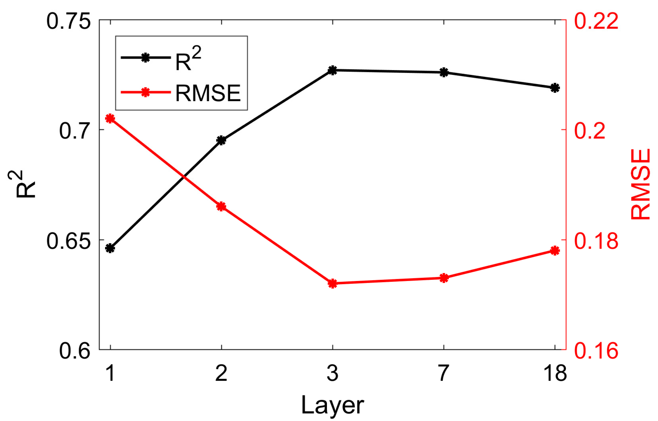
5.4. Sensitivity to the DNN Structure

Generally, the more complicated the DNN structure, the more representative the estimates will be. However, a more complicated DNN structure requires more training samples for stability and reliability. To find the optimum between the number of hidden layers and representativeness, different numbers of hidden layers (1, 2, 3, 7, and 18) were tested. The number of neurons in each hidden layer is shown in Table 3. The 1- and 2-hidden layer models are just simplified versions of the 3-hidden layer model described in Section 3. The 18-hidden layer model is derived by adapting the state-of-the-art Visual Geometry Group (VGG) model developed by the Oxford University [51] by changing all the convolution layers to plain fully connected layers and the 7-hidden layer model is its simplified version (Table 3). The results are as expected (Figure 9), i.e., the accuracy increases with the number of layers initially but levels off when more than 3-hidden-layers are introduced. To use more complicated DNN, e.g., a 7-hidden-layer model, future research with more training samples should be conducted.

6. Conclusions

A DNN algorithm to retrieve AOD from Himawari-8 AHI TOA reflectances has been presented. The six band TOA reflectances, three ratios derived from TOA reflectance, the sun-senor geometries, the reanalysis water vapor and O3 concentrations, and the DEM, which are also used in RTM-based AOD retrievals, are used as DNN predictors. One year (2017) of collocated Level 1 AHI TOA and Version 3 Level 2.0 AERONET AOD observations over the Himawari-8 full disk were used to derive the training and validation samples. The DNN was trained with state-of-the-art techniques and applied to independent validation samples that were not used in the training. The cross-validation is used to reduce the sample variability in randomly sampled training data. The results were compared with those from a random forest regression algorithm and with the JMA AOD products. The following conclusions can be drawn:
(1)
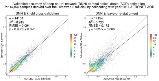
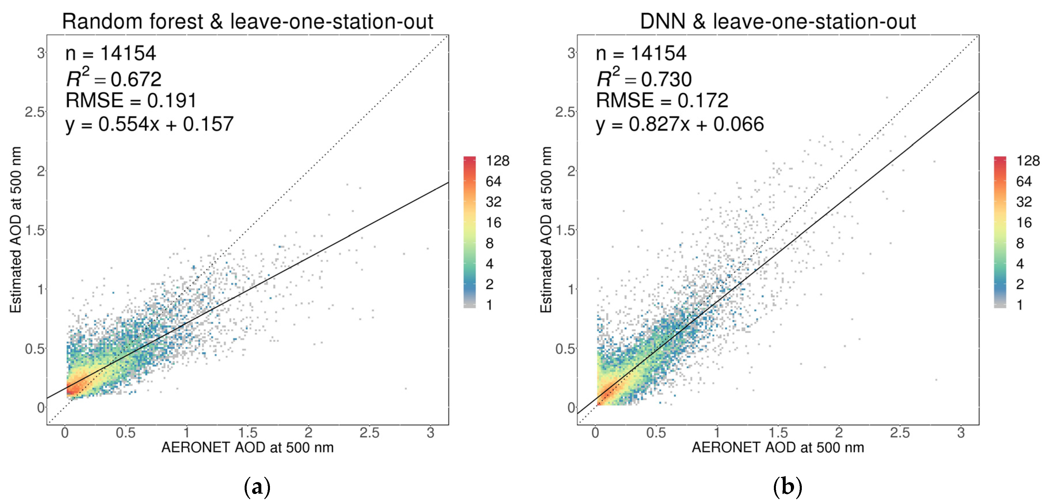
The leave-one-station-out validation shows the capability of the DNN algorithm for systemic AOD retrieval over large-areas using AHI data (RMSE = 0.172, R2 = 0.730).
(2)
The k-fold cross-validation with RMSE = 0.094 and R2 = 0.915 overestimates the accuracy for large-area applications.
(3)
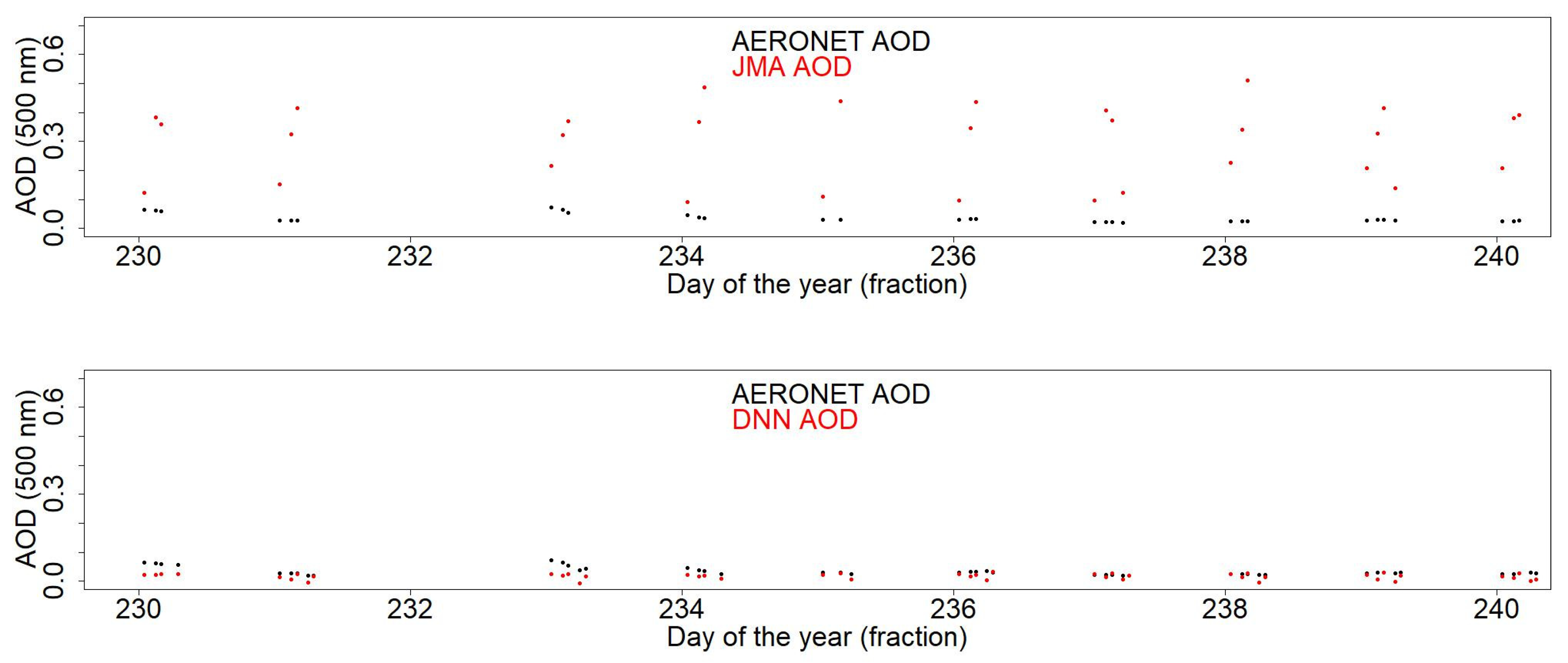
DNN estimated AOD agrees better with AERONET measurements than random forest AOD estimates and the JMA official AOD product.
(4)
Some variables that are important for physical model-based AOD estimation can also improve the DNN AOD estimation. It highlights the importance of the domain knowledge and expertise when using data driven models for aerosol estimation.
The DNN machine learning method does not use assumptions on the surface reflectance and aerosol models. Future work is encouraged to examine how to use the aerosol model assumptions to help improve data-driven-based AOD predictions. One possible way is to train multiple DNN models each applied for a particular aerosol model which can be predefined based on the location geography and climate characteristics.

Author Contributions

Conceptualization, L.S. and H.K.Z.; methodology, L.S. and H.K.Z.; software, L.S.; validation, L.S., H.K.Z. and G.d.L.; formal analysis, L.S.; writing—original draft preparation, L.S. and H.K.Z.; writing—review and editing, H.K.Z., Z.L., G.d.L. and B.H.; visualization, L.S.; funding acquisition, L.S. All authors have read and agreed to the published version of the manuscript.

Funding

This work was supported in part by Open Fund of the State Key Laboratory of Remote Sensing Science (Grant No. OFSLRSS201912). We gratefully acknowledge the support from the Science and Technology Department of Ningxia under grant No. 2019BEB04009.

Acknowledgments

AHI data were supplied by the P-Tree System, Japan Aerospace Exploration Agency (http://www.eorc.jaxa.jp/ptree/terms.html). The authors would like to thank the principal investigators of the AERONET sites used in this paper for maintaining their sites and making their data publicly available.

Conflicts of Interest

The authors declare no conflict of interest.

Appendix A

Table A1. The AERONET sites name, location, number of collocated AHI TOA and AERONET AOD samples and number of days in 2017 with collocated samples. The results are shown for the 76 sites with at least one collocated AHI TOA and AERONET AOD observation pair in 2017.
AERONET Site(Latitude (°), Longitude (°))Number of Collocated SamplesNumber of Days in 2017 with Collocated Samples
Anmyon(36.539, 126.330)4818
ARM_Macquarie_Is(−54.500, 158.935)2519
Bac_Lieu(9.280, 105.730)8747
Bamboo(25.187, 121.535)22
Bandung(−6.888, 107.610)5953
Banqiao(24.998, 121.442)6641
Beijing(39.977, 116.381)351121
Beijing-CAMS(39.933, 116.317)596207
Bhola(22.227, 90.756)19480
Birdsville(−25.899, 139.346)822230
BMKG_GAW_PALU(−1.650, 120.183)11
Bukit_Kototabang(−0.202, 100.318)2819
Canberra(−35.271, 149.111)217108
Cape_Fuguei_Station(25.298, 121.538)11065
Chen-Kung_Univ(22.993, 120.205)313136
Chiang_Mai_Met_Sta(18.771, 98.973)24052
Chiayi(23.496, 120.496)250132
Chiba_University(35.625, 140.104)216102
Dalanzadgad(43.577, 104.419)367166
Dhaka_University(23.728, 90.398)18391
Doi_Inthanon(18.590, 98.486)8745
Dongsha_Island(20.699, 116.729)5831
Douliu(23.712, 120.545)17591
EPA-NCU(24.968, 121.185)20078
Fowlers_Gap(−31.086, 141.701)805230
Fukuoka(33.524, 130.475)7767
Gandhi_College(25.871, 84.128)3719
Gangneung_WNU(37.771, 128.867)519185
Gwangju_GIST(35.228, 126.843)21085
Hankuk_UFS(37.339, 127.266)580194
Hokkaido_University(43.076, 141.341)13663
Hong_Kong_PolyU(22.303, 114.180)44
Irkutsk(51.800, 103.087)16679
Jabiru(−12.661, 132.893)19385
Jambi(−1.632, 103.642)22
Kanpur(26.513, 80.232)349168
KORUS_Kyungpook_NU(35.890, 128.606)6432
KORUS_Mokpo_NU(34.913, 126.437)22
KORUS_UNIST_Ulsan(35.582, 129.190)6919
Kuching(1.491, 110.349)1311
Lake_Argyle(−16.108, 128.749)13865
Lake_Lefroy(−31.255, 121.705)5238
Learmonth(−22.241, 114.097)22
Luang_Namtha(20.931, 101.416)341144
Lulin(23.469, 120.874)6434
Lumbini(27.490, 83.280)19473
Makassar(−4.998, 119.572)235100
Mandalay_MTU(21.973, 96.186)404111
Manila_Observatory(14.635, 121.078)139
ND_Marbel_Univ(6.496, 124.843)4121
NhaTrang(12.205, 109.206)42
Niigata(37.846, 138.942)283106
Nong_Khai(17.877, 102.717)11648
Noto(37.334, 137.137)7633
Omkoi(17.798, 98.432)368117
Osaka(34.651, 135.591)9369
Palangkaraya(−2.228, 113.946)5937
Pioneer_JC(1.384, 103.755)8448
Pokhara(28.1867, 83.975)717246
Pontianak(0.075, 109.191)75
Pusan_NU(35.235, 129.082)7125
QOMS_CAS(28.365, 86.948)1512
Seoul_SNU(37.458, 126.951)455158
Shirahama(33.694, 135.357)107
Silpakorn_Univ(13.819, 100.041)30995
Singapore(1.2977, 103.780)16493
Son_La(21.332, 103.905)6333
Songkhla_Met_Sta(7.184, 100.605)21395
Tai_Ping(10.376, 114.362)331109
Taipei_CWB(25.015, 121.538)11061
Tomsk(56.475, 85.048)116
Tomsk_22(56.417, 84.074)5222
USM_Penang(5.358, 100.302)3824
Ussuriysk(43.700, 132.163)227109
XiangHe(39.754, 116.962)27487
Yonsei_University(37.564, 126.935)599195

References

  1. Stocker, T. Climate Change 2013: The Physical Science Basis: Working Group I Contribution to the Fifth Assessment Report of the Intergovernmental Panel on Climate Change; Cambridge University Press: Cambridge, UK, 2014. [Google Scholar]
  2. Lee, K.H.; Li, Z.; Kim, Y.J.; Kokhanovsky, A. Atmospheric Aerosol Monitoring from Satellite Observations: A History of Three Decades. In Atmospheric and Biological Environmental Monitoring; Springer: Dordrecht, The Netherlands, 2009; pp. 13–38. [Google Scholar]
  3. Kokhanovsky, A.A.; de Leeuw, G. Satellite Aerosol Remote Sensing over Land; Springer: Berlin/Heidelberg, Germany, 2009. [Google Scholar]
  4. Sogacheva, L.; Popp, T.; Sayer, A.M.; Dubovik, O.; Garay, M.J.; Heckel, A.; Hsu, N.C.; Jethva, H.; Kahn, R.A.; Kolmonen, P.; et al. Merging regional and global aerosol optical depth records from major available satellite products. Atmos. Chem. Phys. 2020, 20, 2031–2056. [Google Scholar] [CrossRef] [Green Version]
  5. Kaufman, Y.J.; Tanré, D.; Remer, L.A.; Vermote, E.F.; Chu, A.; Holben, B.N. Operational remote sensing of tropospheric aerosol over land from EOS moderate resolution imaging spectroradiometer. J. Geophys. Res. Atmos. 1997, 102, 17051–17067. [Google Scholar] [CrossRef]
  6. Levy, R.C.; Mattoo, S.; Munchak, L.A.; Remer, L.A.; Sayer, A.M.; Patadia, F.; Hsu, N.C. The collection 6 MODIS aerosol products over land and ocean. Atmos. Meas. Tech. 2013, 6, 2989–3034. [Google Scholar] [CrossRef] [Green Version]
  7. Veefkind, J.P.; de Leeuw, G.; Durkee, P.A. Retrieval of aerosol optical depth over land using two-angle view satellite radiometry during TARFOX. Geophys. Res. Lett. 1998, 25, 3135–3138. [Google Scholar] [CrossRef]
  8. Kahn, R.A.; Gaitley, B.J.; Garay, M.J. Multiangle imaging spectroradiometer global aerosol product assessment by comparison with the aerosol robotic network. J. Geophys. Res. Atmos. 2010, 115, D23. [Google Scholar] [CrossRef]
  9. Holzer-Popp, T.; de Leeuw, G.; Griesfeller, J.; Martynenko, D.; Klüser, L.; Bevan, S.; Davies, W.; Ducos, F.; Deuzé, J.L.; Graigner, R.G. Aerosol retrieval experiments in the ESA aerosol_cci project. Atmos. Meas. Tech. 2013, 6, 1919–1957. [Google Scholar] [CrossRef] [Green Version]
  10. Dubovik, O.; Li, Z.; Mishchenko, M.I.; Tanre, D.; Karol, Y.; Bojkov, B.; Gu, X. Polarimetric remote sensing of atmospheric aerosols: Instruments, methodologies, results, and perspectives. J. Quant. Spectrosc. Radiat. Transfer. 2019, 224, 474–511. [Google Scholar] [CrossRef]
  11. Yoshida, M.; Kikuchi, M.; Nagao, T.M.; Murakami, H.; Nomaki, T.; Higurashi, A. Common retrieval of aerosol properties for imaging satellite sensors. J. Meteorol. Soc. Jpn. Ser. II 2018, 96B, 193–209. [Google Scholar] [CrossRef] [Green Version]
  12. Hsu, N.C.; Tsay, S.C.; King, M.D.; Herman, J.R. Aerosol properties over bright-reflecting source regions. IEEE Trans. Geosci. Remote Sens. 2004, 42, 557–569. [Google Scholar] [CrossRef]
  13. Sayer, A.M.; Hsu, N.C.; Bettenhausen, C.; Jeong, M.J. Validation and uncertainty estimates for MODIS Collection 6 “deep Blue” aerosol data. J. Geophys. Res. Atmos. 2013, 118, 7864–7872. [Google Scholar] [CrossRef] [Green Version]
  14. Sayer, A.M.; Munchak, L.A.; Hsu, N.C.; Levy, R.C.; Bettenhausen, C.; Jeong, M.J. MODIS collection 6 aerosol products: Comparison between aqua’s e-deep blue, dark target, and “merged” data sets, and usage recommendations. J. Geophys. Res. Atmos. 2014, 119, 13965–13989. [Google Scholar] [CrossRef]
  15. Sayer, A.M.; Hsu, N.C.; Bettenhausen, C.; Jeong, M.; Meister, G.; Al, S.E.T. Effect of MODIS terra radiometric calibration improvements on collection 6 deep blue aerosol products: Validation and terra/aqua consistency. J. Geophys. Res. Atmos. 2015, 120, 12157–12174. [Google Scholar] [CrossRef] [Green Version]
  16. Ge, B.; Li, Z.; Liu, L.; Yang, L.; Chen, X.; Hou, W.; Zhang, Y.; Li, D.; Li, L.; Qie, L. A dark target method for Himawari-8/AHI aerosol retrieval: Application and validation. IEEE Trans. Geosci. Remote Sens. 2018, 57, 381–394. [Google Scholar] [CrossRef]
  17. Yang, F.; Wang, Y.; Tao, J.; Wang, Z.; Fan, M.; de Leeuw, G.; Chen, L. Preliminary investigation of a new AHI aerosol optical depth (AOD) retrieval algorithm and evaluation with multiple source AOD measurements in china. Remote Sens. 2018, 10, 748. [Google Scholar] [CrossRef] [Green Version]
  18. Li, S.; Wang, W.; Hashimoto, H.; Xiong, J.; Vandal, T.; Yao, J.; Nemani, R. First provisional land surface reflectance product from geostationary satellite Himawari-8 AHI. Remote Sens. 2019, 11, 2990. [Google Scholar] [CrossRef] [Green Version]
  19. She, L.; Zhang, H.; Wang, W.; Wang, Y.; Shi, Y. Evaluation of the multi-angle implementation of atmospheric correction (MAIAC) aerosol algorithm for Himawari-8 Data. Remote Sens. 2019, 11, 2771. [Google Scholar] [CrossRef] [Green Version]
  20. Lyapustin, A.; Wang, Y.; Laszlo, I.; Kahn, R.; Korkin, S.; Remer, L.; Levy, R.; Reid, J.S. Multiangle implementation of atmospheric correction (MAIAC): 2. aerosol algorithm. J. Geophys. Res. Atmos. 2011, 116, D03211. [Google Scholar] [CrossRef]
  21. Lyapustin, A.; Wang, Y.; Korkin, S.; Huang, D. MODIS collection 6 MAIAC algorithm. Atmos. Meas. Tech. 2018, 11, 5741–5765. [Google Scholar] [CrossRef] [Green Version]
  22. LeCun, Y.; Bengio, Y.; Hinton, G. Deep learning. Nature 2015, 521, 436–444. [Google Scholar] [CrossRef]
  23. Holben, B.N.; Eck, T.F.; Slutsker, I.; Tanre, D.; Buis, J.P.; Setzer, A.; Vermote, E.; Reagan, J.A.; Kaufman, Y.J.; Nakajima, T.; et al. AERONET—A federated instrument network and data archive for aerosol characterization. Remote Sens. Environ. 1998, 66, 1–16. [Google Scholar] [CrossRef]
  24. Vucetic, S.; Han, B.; Mi, W.; Li, Z.; Obradovic, Z. A data-mining approach for the validation of aerosol retrievals. IEEE Geosci. Remote Sens. Lett. 2008, 5, 113–117. [Google Scholar] [CrossRef] [Green Version]
  25. Radosavljevic, V.; Vucetic, S.; Obradovic, Z. A data-mining technique for aerosol retrieval across multiple accuracy measures. IEEE Geosci. Remote Sens. Lett. 2010, 7, 411–415. [Google Scholar] [CrossRef] [Green Version]
  26. Ristovski, K.; Vucetic, S.; Obradovic, Z. Uncertainty analysis of neural-network-based aerosol retrieval. IEEE Trans. Geosci. Remote Sens. 2012, 50, 409–414. [Google Scholar] [CrossRef]
  27. Kolios, S.; Hatzianastassiou, N. Quantitative aerosol optical depth detection during dust outbreaks from METEOSAT imagery using an artificial neural network model. Remote Sens. 2019, 11, 1022. [Google Scholar] [CrossRef] [Green Version]
  28. Lary, D.J.; Remer, L.A.; MacNeill, D.; Roscoe, B.; Paradise, S. Machine learning and bias correction of MODIS aerosol optical depth. IEEE Trans. Geosci. Remote Sens. 2009, 6, 694–698. [Google Scholar] [CrossRef] [Green Version]
  29. Just, A.C.; de Carli, M.M.; Shtein, A.; Dorman, M.; Lyapustin, A.; Kloog, I. Correcting measurement error in satellite aerosol optical depth with machine learning for modeling PM2. 5 in the Northeastern USA. Remote Sens. 2018, 10, 803. [Google Scholar] [CrossRef] [Green Version]
  30. Li, L. A robust deep learning approach for spatiotemporal estimation of satellite AOD and PM2.5. Remote Sens. 2020, 12, 264. [Google Scholar] [CrossRef] [Green Version]
  31. Su, T.; Laszlo, I.; Li, Z.; Wei, J.; Kalluri, S. Refining aerosol optical depth retrievals over land by constructing the relationship of spectral surface reflectances through deep learning: Application to Himawari-8. Remote Sens. Environ. 2020, 251, 112093. [Google Scholar] [CrossRef]
  32. Chen, X.; de Leeuw, G.; Arola, A.; Liu, S.; Liu, Y.; Li, Z.; Zhang, K. Joint retrieval of the aerosol fine mode fraction and optical depth using MODIS spectral reflectance over northern and eastern China: Artificial neural network method. Remote Sens. Environ. 2020, 249, 112006. [Google Scholar] [CrossRef]
  33. Stafoggia, M.; Bellander, T.; Bucci, S.; Davoli, M.; de Hoogh, K.; de’Donato, F.; Scortichini, M. Estimation of daily PM10 and PM2. 5 concentrations in Italy, 2013–2015, using a spatiotemporal land-use random-forest model. Environ. Int. 2019, 124, 170–179. [Google Scholar] [CrossRef]
  34. Choubin, B.; Abdolshahnejad, M.; Moradi, E.; Querol, X.; Mosavi, A.; Shamshirband, S.; Ghamisi, P. Spatial hazard assessment of the PM10 using machine learning models in Barcelona, Spain. Sci. Total Environ. 2020, 701, 134474. [Google Scholar] [CrossRef] [PubMed]
  35. Wei, J.; Huang, W.; Li, Z.; Xue, W.; Peng, Y.; Sun, L.; Cribb, M. Estimating 1-km-resolution PM2.5 concentrations across China using the space-time random forest approach. Remote Sens. Environ. 2019, 231, 111221. [Google Scholar] [CrossRef]
  36. Dong, L.; Li, S.; Yang, J.; Shi, W.; Zhang, L. Investigating the performance of satellite-based models in estimating the surface PM2. 5 over China. Chemosphere 2020, 256, 127051. [Google Scholar] [CrossRef] [PubMed]
  37. Okuyama, A.; Andou, A.; Date, K.; Hoasaka, K.; Mori, N.; Murata, H.; Tabata, T.; Takahashi, M.; Yoshino, R.; Bessho, K.; et al. Preliminary validation of Himawari-8/AHI navigation and calibration. Earth Obs. Syst. 2015, 9607, 96072E. [Google Scholar]
  38. Okuyama, A.; Takahashi, M.; Date, K.; Hosaka, K.; Murata, H.; Tabata, T.; Yoshino, R. Validation of Himawari-8/AHI radiometric calibration based on two years of In-Orbit data. J. Meteorol. Soc. Jpn. Ser. II 2018, 96, 91–109. [Google Scholar] [CrossRef] [Green Version]
  39. Nakajima, T.; Tanaka, M. Matrix formulations for the transfer of solar radiation in a plane-parallel scattering atmosphere. J. Quant. Spectrosc. Radiat. Transfer. 1986, 35, 13–21. [Google Scholar] [CrossRef]
  40. Russell, P.B.; Livingston, J.M.; Dutton, E.G.; Pueschel, R.F.; Reagan, J.A.; Defoor, T.E.; Box, M.A.; Allen, D.; Pilewskie, P.; Herman, B.M.; et al. Pinatubo and pre-Pinatubo optical-depth spectra: Mauna Loa measurements, comparisons, inferred particle size distributions, radiative effects, and relationship to lidar data. J. Geophys. Res. Atmos. 1993, 98, 22969–22985. [Google Scholar] [CrossRef]
  41. Giles, D.M.; Sinyuk, A.; Sorokin, M.G.; Schafer, J.S.; Smirnov, A.; Slutsker, I.; Eck, T.F.; Holben, B.N.; Lewis, J.R.; Campbell, J.R.; et al. Advancements in the aerosol robotic network (AERONET) version 3 database–automated near-real-time quality control algorithm with improved cloud screening for sun photometer aerosol optical depth (AOD) measurements. Atmos. Meas. Tech. 2019, 12, 169–209. [Google Scholar] [CrossRef] [Green Version]
  42. Hsu, N.C.; Jeong, M.J.; Bettenhausen, C.; Sayer, A.M.; Hansell, R.; Seftor, C.S.; Huang, J.; Tsay, S.C. Enhanced DB aerosol retrieval algorithm: The second generation. J. Geophys. Res. Atmos. 2013, 118, 9296–9315. [Google Scholar] [CrossRef]
  43. Bohren, C.F.; Huffman, D.R. Absorption and Scattering of Light by Small Particles; Wiley & Sons: Hoboken, NJ, USA, 1983. [Google Scholar]
  44. Li, Z.; Zhang, H.K.; Roy, D.P. Investigation of Sentinel-2 bidirectional reflectance hot-spot sensing conditions. IEEE Trans. Geosci. Remote Sens. 2019, 57, 3591–3598. [Google Scholar] [CrossRef]
  45. Liang, S.L. Quantitative Remote Sensing of Land Surface; Wiley & Sons: Hoboken, NJ, USA, 2004. [Google Scholar]
  46. Yuan, Q.; Shen, H.; Li, T.; Li, Z.; Li, S.; Jiang, Y.; Gao, J. Deep learning in environmental remote sensing: Achievements and challenges. Remote Sens. Environ. 2020, 241, 111716. [Google Scholar] [CrossRef]
  47. Glorot, X.; Bordes, A.; Bengio, Y. Deep sparse rectifier neural networks. In Proceedings of the Fourteenth International Conference on Artificial Intelligence and Statistics, Fort Lauderdale, FL, USA, 11–13 April 2011; pp. 315–323. [Google Scholar]
  48. Ruder, S. An Overview of Gradient Descent Optimization Algorithms; Insight Centre for Data Analytics: Dublin, Ireland, 2016. [Google Scholar]
  49. He, K.; Zhang, X.; Ren, S.; Sun, J. Deep residual learning for image recognition. In Proceedings of the IEEE Conference on Computer Vision and Pattern Recognition, Las Vegas, NV, USA, 27–30 June 2016; pp. 770–778. [Google Scholar]
  50. Krizhevsky, A.; Sutskever, I.; Hinton, G.E. Imagenet classification with deep convolutional neural networks. In Proceedings of the 25th International Conference on Neural Information Processing Systems, Toronto, ON, Canada, 1 December 2012; pp. 1097–1105. [Google Scholar]
  51. Simonyan, K.; Zisserman, A. Very deep convolutional networks for large-scale image recognition. In Proceedings of the International Conference on Learning Representations, Oxford, UK, 14–16 April 2014. [Google Scholar]
  52. Iandola, F.N.; Han, S.; Moskewicz, M.W.; Ashraf, K.; Dally, W.J.; Keutzer, K. SqueezeNet: AlexNet-Level Accuracy with 50x Fewer Parameters and<0.5 MB Model Size. arXiv 2016, arXiv:1602.07360. [Google Scholar]
  53. Dong, C.; Loy, C.C.; He, K.; Tang, X. Image super-resolution using deep convolutional networks. IEEE Trans. Pattern Anal. Mach. Intell. 2016, 38, 295–307. [Google Scholar] [CrossRef] [PubMed] [Green Version]
  54. He, K.; Zhang, X.; Ren, S.; Sun, J. Delving Deep into Rectifiers: Surpassing Human-Level Performance on Imagenet Classification. In Proceedings of the IEEE International Conference on Computer Vision, Santiago, Chile, 7–13 December 2015; pp. 1026–1034. [Google Scholar]
  55. Ioffe, S.; Szegedy, C. Batch Normalization: Accelerating Deep Network Training by Reducing Internal Covariate Shift; Google: Mountain View, CA, USA, 2015. [Google Scholar]
  56. Abadi, M.; Agarwal, A.; Barham, P.; Brevdo, E.; Chen, Z.; Citro, C.; Ghemawat, S. Tensorflow: Large-Scale Machine Learning on Heterogeneous Distributed Systems. 2016. Available online: https://static.googleusercontent.com/media/research.google.com/en//pubs/archive/45166.pdf (accessed on 16 December 2020).
  57. Rodriguez, J.D.; Perez, A.; Lozano, J.A. Sensitivity analysis of k-fold cross validation in prediction error estimation. IEEE Trans. Pattern Anal. Mach. Intell. 2010, 32, 569–575. [Google Scholar] [CrossRef]
  58. Gupta, P.; Christopher, S.A. Particulate matter air quality assessment using integrated surface, satellite, and meteorological products: Multiple regression approach. J. Geophys. Res. Atmos. 2009, 114, D14. [Google Scholar] [CrossRef] [Green Version]
  59. Hu, X.; Waller, L.A.; Lyapustin, A.; Wang, Y.; Al-Hamdan, M.Z.; Crosson, W.L.; Liu, Y. Estimating ground-level PM2. 5 concentrations in the Southeastern United States using MAIAC AOD retrievals and a two-stage model. Remote Sens. Environ. 2014, 140, 220–232. [Google Scholar] [CrossRef]
  60. He, Q.; Huang, B. Satellite-based mapping of daily high-resolution ground PM2. 5 in China via space-time regression modeling. Remote Sens. Environ. 2018, 206, 72–83. [Google Scholar] [CrossRef]
  61. Kloog, I.; Nordio, F.; Coull, B.A.; Schwartz, J. Incorporating local land use regression and satellite aerosol optical depth in a hybrid model of spatiotemporal PM2. 5 exposures in the Mid-Atlantic states. Environ. Sci. Technol. 2012, 46, 11913–11921. [Google Scholar] [CrossRef] [Green Version]
  62. Li, T.; Shen, H.; Yuan, Q.; Zhang, X.; Zhang, L. Estimating ground-level PM2. 5 by fusing satellite and station observations: A geo-intelligent deep learning approach. Geophy. Res. Lett. 2017, 44, 11–985. [Google Scholar] [CrossRef] [Green Version]
  63. Liaw, A.; Wiener, M. Classification and regression by randomForest. R News 2002, 2, 18–22. [Google Scholar]
  64. Belgiu, M.; Drăguţ, L. Random forest in remote sensing: A review of applications and future directions. ISPRS J. Photogramme. Remote Sens. 2016, 114, 24–31. [Google Scholar] [CrossRef]
  65. Hu, X.; Belle, J.H.; Meng, X.; Wildani, A.; Waller, L.A.; Strickland, M.J.; Liu, Y. Estimating PM2.5 concentrations in the conterminous United States using the random forest approach. Environ. Sci. Technol. 2017, 51, 6936–6944. [Google Scholar] [CrossRef] [PubMed]
  66. Chen, J.; Yin, J.; Zang, L.; Zhang, T.; Zhao, M. Stacking machine learning model for estimating hourly PM2.5 in China based on Himawari 8 aerosol optical depth data. Sci. Total Environ. 2019, 697, 134021. [Google Scholar] [CrossRef] [PubMed]
  67. Zuo, X.; Guo, H.; Shi, S.; Zhang, X. Comparison of six machine learning methods for estimating PM2.5 concentration using the Himawari-8 aerosol optical depth. J. Indian Soc. Remote 2020, 48, 1277–1287. [Google Scholar] [CrossRef]
  68. Remer, L.A.; Kleidman, R.G.; Levy, R.C.; Kaufman, Y.J.; Tanré, D.; Mattoo, S.; Holben, B.N. Global aerosol climatology from the MODIS satellite sensors. J. Geophys. Res. Atmos. 2008, 113, D14. [Google Scholar] [CrossRef] [Green Version]
  69. Mao, K.B.; Ma, Y.; Xia, L.; Chen, W.Y.; Shen, X.Y.; He, T.J.; Xu, T.R. Global aerosol change in the last decade: An analysis based on MODIS data. Atmos. Environ. 2014, 94, 680–686. [Google Scholar] [CrossRef] [Green Version]
  70. Ju, J.; Roy, D.P.; Vermote, E.; Masek, J.; Kovalskyy, V. Continental-scale validation of MODIS-based and LEDAPS Landsat ETM + atmospheric correction methods. Remote Sens. Environ. 2012, 122, 175–184. [Google Scholar] [CrossRef] [Green Version]
  71. Ramachandran, S.; Rupakheti, M.; Lawrence, M.G. Black carbon dominates the aerosol absorption over the indo-gangetic plain and the Himalayan foothills. Environ. Int. 2020, 142, 105814. [Google Scholar] [CrossRef]
  72. Xie, B.; Zhang, H.K.; Xue, J. Deep convolutional neural network for mapping smallholder agriculture using high spatial resolution satellite image. Sensors 2019, 19, 2398. [Google Scholar] [CrossRef] [Green Version]
  73. Wieland, M.; Li, Y.; Martinis, S. Multi-sensor cloud and cloud shadow segmentation with a convolutional neural network. Remote Sens. Environ. 2019, 230, 111203. [Google Scholar] [CrossRef]
  74. Zhang, B.; Zhao, L.; Zhang, X. Three-dimensional convolutional neural network model for tree species classification using airborne hyperspectral images. Remote Sens. Environ. 2020, 247, 111938. [Google Scholar] [CrossRef]
  75. Breiman, L. Random forests. Mach. Learn. 2001, 45, 5–32. [Google Scholar] [CrossRef] [Green Version]
  76. Loh, W.Y. Classification and Regression Trees; Wiley & Sons: Hoboken, NJ, USA, 2011; pp. 14–23. [Google Scholar]
  77. Wei, J.; Li, Z.; Sun, L.; Peng, Y.; Zhang, Z.; Li, Z.; Su, T.; Feng, L.; Cai, Z.; Wu, H. Evaluation and uncertainty estimate of next-generation geostationary meteorological Himawari-8/AHI aerosol products. Sci. Total Environ. 2019, 692, 879–891. [Google Scholar] [CrossRef] [PubMed]
  78. Gupta, P.; Remer, L.A.; Levy, R.C.; Mattoo, S. Validation of MODIS 3 km land aerosol optical depth from NASA’s EOS terra and aqua missions. Atmos. Meas. Tech. 2018, 11, 3145–3159. [Google Scholar] [CrossRef] [Green Version]
Figure 1. k-fold cross-validation of the estimated AOD (k = 76) using random forest (a) and the 3-hidden layer deep neural network (DNN) (b). The values of the colors (see color scale to the right of each plot) indicate the frequency of occurrence of similar AOD values binned by 0.015 (200 bins in both x and y directions).
Remotesensing 12 04125 g001
Figure 2. Leave one station out validation of the estimated 500 nm AOD using random forest (a) and the 3-hidden layer DNN (b). The values of the colors (see color scale to the right of each plot) indicate the frequency of occurrence of similar AOD values binned by 0.015 (200 bins in both x and y directions).
Remotesensing 12 04125 g002
Figure 3. Map of the study area with AERONET stations color-coded according to the root-mean-square deviation (RMSE) for the DNN leave-one-station-out AOD validation at that site. A few sites around the South China Sea are located at islands (e.g., Dongsha island and Tai-Ping island).
Remotesensing 12 04125 g003
Figure 4. Comparison of Japan Meteorological Agency (JMA) AOD (a) and the DNN estimated AOD (b) validation versus AERONET, using the leave-one-station-out sampling strategy. The values of the colors (see color scale to the right of each plot) indicate the frequency of occurrence of similar AOD values binned by 0.015 (200 bins in both x and y directions).
Remotesensing 12 04125 g004
Figure 5. AOD time series (days 230 to 240 of year 2017) at the Birdsville AERONET station (Australia) showing (top) the AERONET 500 nm AOD (black dots) and the JMA 500 nm AOD (red dots) values, (bottom) the AERONET AOD (black dots) and the DNN AOD (red dots) values.
Remotesensing 12 04125 g005
Figure 6. Same as Figure 5 but for days 310 to 320 of the year 2017 for the Pokhara AERONET station (Nepal).
Remotesensing 12 04125 g006
Figure 7. An example station (Fowlers_Gap station in Australia) showing the significantly better k-fold cross-validation (a) than the leave-one-station-out validation (b). The values of the colors (see color scale to the right of each plot) indicate the frequency of occurrence of similar AOD values binned by 0.003 (200 bins in both x and y directions).
Remotesensing 12 04125 g007
Figure 8. Density scatterplot of the DNN estimated AOD without using the three TOA reflectance ratio predictors versus AERONET AOD, using the leave-one-station-out sampling strategy with only 14 predictors, i.e., the same as Figure 2b but excluding the three TOA reflectance ratio predictors. The values of the colors (see color scale to the right of the plot) indicate the frequency of occurrence of similar AOD values binned by 0.015 (200 bins in both x and y directions).
Remotesensing 12 04125 g008
Figure 9. AOD estimation R2 and RMSE as a function of the number of DNN hidden layers using leave-one-station-out validation.
Remotesensing 12 04125 g009
Table 1. Central wavelengths and spatial resolutions of bands 1–6 of Himawari L1 data (http://www.jma-net.go.jp/msc/en/).
Band NumberCentral Wavelength (μm)Band NameSpatial Resolution (km)
10.47blue2
20.51green2
30.64red2
40.86near infrared (NIR)2
51.61shortwave infrared (SWIR)2
62.25SWIR2
Table 2. Descriptive statistics for AErosol RObotic NETwork (AERONET) aerosol optical depth (AOD) and predictor variables. The units for view/solar zenith/azimuth angle, water vapor content and ozone content are degrees, kg m−2 and kg m−2 respectively. AOD and top of atmosphere (TOA) reflectance are unitless.
MeanStdMinMax
AERONET AOD 500 nm0.300.320.00 2.98
TOA band 10.220.060.080.45
TOA band 20.190.060.060.43
TOA band 30.170.060.030.46
TOA band 40.280.080.020.71
TOA band 50.240.100.010.55
TOA band 60.140.070.000.38
View zenith angle46.4711.9517.3669.60
View azimuth angle109.3955.81−179.03179.11
Solar zenith angle44.5915.311.7170.12
Solar azimuth angle−0.23125.49−179.97179.93
Water vapor content22.9116.310.5166.95
Ozone content6.30 × 10−39.79 × 10−44.80 × 10−31.07 × 10⁻²
Table 3. The different CNN structures and their numbers of hidden neurons in each layer. These neuron numbers are used in the classical convolutional neural network models in the computer vision field [51,53].
Number of Hidden LayersNumber of Neurons in Each Hidden Layer
1-hidden-layer256
2-hidden-layer256, 512
3-hidden-layer (Section 3)256, 512, 512
7-hidden-layer256, 256, 256, 512, 512,1024,1024
18-hidden-layer64, 64, 128, 128, 256, 256, 256, 256, 512, 512, 512, 512, 512, 512, 512, 512, 1024,1024
Publisher’s Note: MDPI stays neutral with regard to jurisdictional claims in published maps and institutional affiliations.

