Rating Iron Deficiency in Soybean Using Image Processing and Decision-Tree Based Models


1
Department of Agricultural and Biosystems Engineering, North Dakota State University, 1221 Albrecht Boulevard, Fargo, ND 58102, USA
2
College of Agriculture & Montana Agricultural Experiment Station, Montana State University, 202 Linfield Hall, Bozeman, MT 59717, USA
*
Author to whom correspondence should be addressed.
Remote Sens. 2020, 12(24), 4143; https://0-doi-org.brum.beds.ac.uk/10.3390/rs12244143
Submission received: 2 November 2020
/
Revised: 13 December 2020
/
Accepted: 16 December 2020
/
Published: 18 December 2020
(This article belongs to the Special Issue Remote and Proximal Sensing for Precision Agriculture and Viticulture)
Abstract
:The most efficient way of soybean (Glycine max (L.) Merrill) iron deficiency chlorosis (IDC) management is to select a tolerant cultivar suitable for the specific growing condition. These cultivars are selected by field experts based on IDC visual ratings. However, this visual rating method is laborious, expensive, time-consuming, subjective, and impractical on larger scales. Therefore, a modern digital image-based method using tree-based machine learning classifier models for rating soybean IDC at plot-scale was developed. Data were collected from soybean IDC cultivar trial plots. Images were processed with MATLAB and corrected for light intensity by using a standard color board in the image. The three machine learning models used in this study were decision tree (DT), random forest (RF), and adaptive boosting (AdaBoost). Calculated indices from images, such as dark green color index (DGCI), canopy size, and pixel counts into DGCI ranges and IDC visual scoring were used as input and target variables to train these models. Metrics such as precision, recall, and f1-score were used to assess the performance of the classifier models. Among all three models, AdaBoost had the best performance (average f1-score = 0.75) followed by RF and DT the least. Therefore, a ready-to-use methodology of image processing with AdaBoost model for soybean IDC rating was recommended. The developed method can be easily adapted to smartphone applications or scaled-up using images from aerial platforms.
1. Introduction
The US is the second largest exporter of soybean and its product in the world with a crop value of over $39 billion in 2018 [1], and the Midwest is one of the biggest production regions. However, soybean production in general and in the Midwest specifically can be declined by iron deficiency chlorosis (IDC). IDC is characterized by a reduction in the chlorophyll of the leaves, which makes the leaves turn from green to yellowish that in consequence interferes with photosynthesis, causing reduced plant height and leaf area [2], which negatively affect the production. For efficient management of soybean IDC, measurement and assessment of the extent of the damage is the key step. The most common and current method employed IDC assessment is the manual visual scoring system by the field experts, where a higher score means increased incidence. This method, however, is laborious, expensive, and time-consuming, as well as subjective. Furthermore, it is impractical to use this method on larger scales. Therefore, a modern method of image processing from the actual field images was proposed, tested, and compared with manual rating in this study.
Among different methods available to combat IDC, such as planting a companion crop [3,4], applying iron chelate [5,6], increasing seeding rate, and planting in wider rows [7], planting tolerant cultivars was proposed as the most effective way to avoid IDC [8,9,10]. Although planting IDC tolerant cultivar reduces IDC incidence, it will not increase the yield throughout the entire field most of the time [11]. For IDC assessment, the commonly followed method is IDC visual score, but it is prone to human inconsistency and is a subjective measurement, which means that different experts may rate plots with different scores. A relatively poor correlation among experts () was observed when experts visually rated turf plots for leaf spot, density, and color [12]. Light conditions in the field also affect the appearance of color and the human perception of color, which in turn will influence the score [13]. The field rating will also be inconsistent because an expert may sometimes rate the same plot with different scores. In a study that was conducted on rating turf plots, raters’ variance of visual rating scores was found significantly higher than the variance of dark green color index (DGCI) from digital images after evaluating the same turf plots for several times [14].
As an alternative to manual visual rating, digital image processing can be used for efficient IDC assessment in field conditions. Digital image processing captures the reflection of light similar to human eyes and is much more objective and expected to be consistent compared to visual rating. These images were used for phenotyping of different crops by extracting different color vegetation indices (CVI) from them [15,16]. Yellow and green disks, components of the standard color board, of known DGCI values, were used to compensate for different lighting conditions and the effect of different sensitivity to colors among various cameras on corn (Zea mays L.) [17]. A close relationship between the amount of nitrogen in corn leaf and DGCI value was reported from that study. Image processing was demonstrated to estimate chlorophyll from soybean leaf images using the DGCI [18].
The CVI values from digital images for IDC rating are continuous, but the visual ratings values are discreet. Advanced machine learning classification algorithms are great models to predict discreet classes, similar to visual scores, based on continuous CVI values. These machine learning methods have been used in many aspects of agriculture, such as yield prediction [19], weed detection [20], iron deficiency rating [21], disease detection in wheat (Triticum aestivum L.) [22], and classifying broad agricultural land cover types [23], to mention a few.
Of the several machine learning methods, identification of the most important field attributes in soybean yield prediction was performed using random forest regression [19]. The random forest model was also used to improve soybean yield estimation and predict soybean maturity through aerial imagery [24]. Among several machine learning classification models, such as decision tree, random forest, and hierarchical model, that were used to rate IDC in soybean five seeds hill plots, under controlled lighting conditions with images captured from above, the hierarchical classifier resulted in the best accuracy [21]. In a similar study, Bai et al. [25] used a platform to capture images of soybean plots from above, without ambient light compensation, and used linear discriminant analysis (LDA) and support vector machine (SVM) to classify the severity of IDC, and found the SVM produced the increased accuracy. They also rated soybean for IDC “in-office” by observing the pictures called office score and found that office score was more consistent in the IDC scoring across different site-years.
Research on soybean IDC rating using image processing in an uncontrolled condition, at actual field plots with lighting compensation, is not found in the literature. Therefore, a research investigation on the application of image processing in determining the IDC, and developing decision-tree based prediction models from the image data at the field plot scale, was proposed. Such combined image processing and machine learning model methodology to efficiently rate soybean IDC that is applicable in the field is novel and will be welcomed by various stakeholders. The specific objectives of this research were: (i) to determine the distribution of IDC visual scoring data and DGCI image information obtained infield along with a standard color board; (ii) to assess several machine learning models on IDC rating; and (iii) to develop ready-to-use prediction methodology from DGCI input. Outputs of the research work will have broader applications and are expected to impact the soybean farmers/producers, breeders, crop consultants, agricultural extension agents, and other users.
2. Materials and Methods
2.1. Field Experimental Plots
Forty different cultivars of soybean were planted in Leonard, ND, USA (46.671783N, 97.245939W) for the IDC tolerant cultivar experiment. The region selected for the experiment is well-known for its soil conditions issues that create soybean IDC, hence selected for the IDC tolerant cultivar evaluation trials. The experimental field of about 3000 m2 (≈1 ac) was divided into four blocks (4 replications) and each block was divided into 40 plots to plant the selected IDC tolerant soybeans (40 cultivars). Thus, 160 plots was considered in the study (4 replications × 40 cultivars = 160 plots; Figure 1). Each plot was 3.4 m long and 3.0 m wide and had four rows with a row spacing of 0.76 m. The plots were seeded at a density of 30 seeds/m in each row in mid-May, 2014. The 1st and 4th rows were the border rows and to avoid the edge effect were not considered, while the 2nd and 3rd rows were only considered for the analysis.
It should be noted that this soybean IDC tolerant cultivar experiments were originally designed and conducted by North Dakota State University (NDSU) agronomists, and experts rated all plots and supplied the visual IDC rating scores. As the entire field side is affected and known to produce soybean IDC symptoms on varieties to varying extent, no “control” treatment plots were identified that will be completely unaffected by IDC. This ongoing experimental trial was just used in this study to develop a methodology (image processing with machine learning) mimicking the visual rating by the experts through images. Furthermore, the selection of cultivars, controls, and the experimental design of the plots are beyond the scope of this study and are not expected to affect the proposed methodology development.
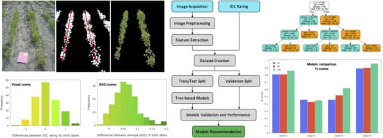
2.2. Overall Methodology
The research aims to apply image processing methodology using field plot images and develop prediction models to determine the IDC classes of soybean. The overall methodology, showing various processes involved in image processing, machine learning model development, and validation for IDC classification, is illustrated in Figure 2. These processes are described in detail subsequently. All the plot images were processed to extract features, such as the two-colored disks and two middle soybean rows. From the middle rows, new features were calculated to serve as input features to develop and train the tree-based models. These models used visual expert’s ratings as the target variable and were tested using classification metrics on a portion of the dataset that was not used in the training of the models.
2.3. IDC Visual Rating
In the experiments, soybeans were visually rated for IDC by experts in 2014 first at the V2–V3 growing stage (3 July) and the second time at the V5–V6 growing stage (17 July). Table 1 shows the developed IDC rating scores used in the experiments [11]. For each rating, visual IDC scores were recorded to the nearest one-half (0.5) unit.
2.4. Image Acquisition
Images of soybean plots were captured on the same days that the expert rated soybean for IDC (3–17 July 2014). To account for differences in ambient lighting and the effect of different cameras on final images, a standard color board was placed between 2nd and 3rd rows in each image that will be later processed (Figure 3). The middle rows (2nd and 3rd) with the standard color board were captured and analyzed for the image-based IDC scoring. A SONY™ DSC-W80 digital camera with an image size of pixels was set to an ISO of 125 in the “Automatic” mode to ensure equal brightness for all images captured. Images were saved as JPEG (Joint Photographic Experts Group) files and numbered based on cameras’ internal numbering sequence.
The images were taken while standing (camera height about 1.7 m) near the end of a plot at a consistent angle so that the whole plot length at the front with pathways on both ends with about 10% of the plot above was captured (Figure 3). To have this coverage, the angle of the centerline of the camera was around 33 from the horizontal line. It should be noted that taking pictures with lower angles or heights can affect canopy size and the amount of information that a camera can record. Given the images were captured consistently for all the plots (camera height, angle, and coverage), the resulting oblique images can be directly processed without the need for any transformation (e.g., orthorectification) as the aim was to measure the color of the soybean plants. Images were processed in MATLAB [26] to extract the desirable features (e.g., vegetation, standard color board, and color disks) and perform various analyses.
Standard colors consisted of yellow and green 90 mm diameter circular disk set on a pink (#eA328A hex; 234, 50, 138 RGB; ![Remotesensing 12 04143 i001]() ) board. The standard HSB values of yellow disk are 50, 87, and 91 (#e7c71f hex; 231, 199, 31 RGB;
) board. The standard HSB values of yellow disk are 50, 87, and 91 (#e7c71f hex; 231, 199, 31 RGB; ![Remotesensing 12 04143 i002]() ) and for green disk are 91, 38, and 42 (#576c43 hex; 87, 108, 67 RGB;
) and for green disk are 91, 38, and 42 (#576c43 hex; 87, 108, 67 RGB; ![Remotesensing 12 04143 i003]() ), which produced the DGCI (Equation (1)) values of 0.0178 for yellow and 0.5722 for green disk [17]. These known DGCI values of disks were used along with the observed values of these disks from the image to calibrate DGCI values of soybeans.
), which produced the DGCI (Equation (1)) values of 0.0178 for yellow and 0.5722 for green disk [17]. These known DGCI values of disks were used along with the observed values of these disks from the image to calibrate DGCI values of soybeans.
 ) board. The standard HSB values of yellow disk are 50, 87, and 91 (#e7c71f hex; 231, 199, 31 RGB;
  ) and for green disk are 91, 38, and 42 (#576c43 hex; 87, 108, 67 RGB;
  ), which produced the DGCI (Equation (1)) values of 0.0178 for yellow and 0.5722 for green disk [17]. These known DGCI values of disks were used along with the observed values of these disks from the image to calibrate DGCI values of soybeans.
The expression of DGCI values for soybean from the HSB color space channels [14] used in the analysis is:
The raw DGCI values (Equation (1)) of the extracted vegetation component of the image needs correction based on the lighting conditions, and this correction was performed using the extracted colors of the disks of the standard color board. For this correction, it is assumed that the known and observed values of DGCI from the camera follow a simple linear relation. The DGCI correction (Equations (2)–(4)) was performed based on the slope and intercept of the assumed linear response as:
2.5. Object Recognition in Field Image
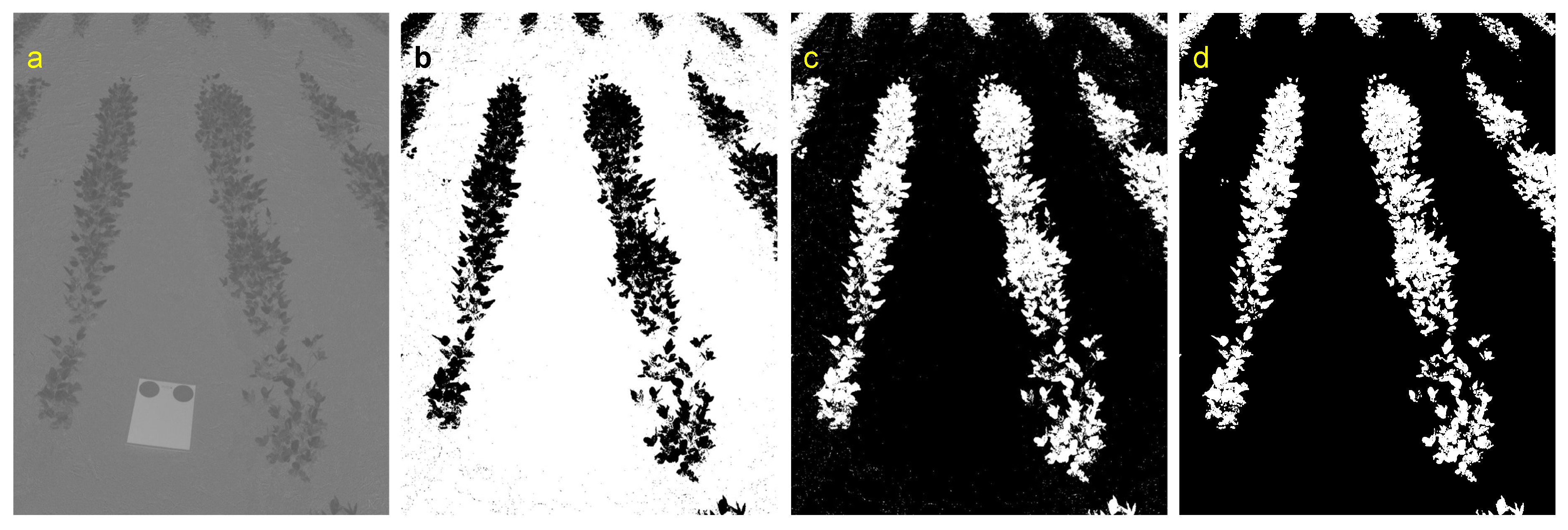
The purpose of object recognition is to detect multiple features from the images (Figure 3) such as middle rows, standard color board, and the colored disks on the board for features extraction required in the analysis. The feature detection and extraction were performed with MATLAB [26] image processing toolbox, which was used in the calculation of DGCI and other input features. Brief description of object recognition is presented subsequently (see Figures 5 and 6).
Images were imported into MATLAB as a 3D matrix with 3 layers of 2D unsigned 8-bit integer matrix, which has layers of red, green, and blue (RGB). In the image preprocessing, grayscale images were created by slicing the original color images to its component layers of RGB (e.g., Red = image(:,:,1)). The pixel values of the grayscale images vary between 0 and 255, where 0 represents absences of the color and is shown by black. Similarly, 255 represents the pure color and is shown by white; everything in between represents different shades of that color (RGB), but are shown with different shades of gray. The brightness of the loaded images was calculated through hue, saturation, brightness (HSB) color space, which is closer to human perception of color and therefore helpful to recognize objects in the images. This image preprocessing is essential for features identification and extraction.
2.5.1. Extraction of Standard Color Board
To recognize and extract the two-color disks of the standard color board that had the reference color information, the color board had to be detected first. The color board can be easily recognized through component (red/green chromatics) of colorspace as the histogram clearly showing three distinct peaks (Figure 4).
The component of the original image is a grayscale image (Figure 5a) that can be used to process several specific binary images. Using the imbinarize() command and proper thresholds (based on the peaks), the binary images were created after recognizing different features. This binary image was used to create a mask for extracting the standard color board using the object’s area property as the board’s area dominates over other artifacts created by leaves. The artifacts were removed using the imopen() command with a “square” structure to both remove the small objects and preserve the shape of the board. In the binary image, it can be seen that the colored disks left holes (Figure 5b) and using bwconvhull() command the holes got filled.
At this stage, the color board was the only object in the binary image (Figure 5c), and its corresponding major and minor axes lengths were extracted using regionprops() command. These lengths were used to estimate the board area to be used for thresholds in later morphological operations. Furthermore, the bounding box of the board was extracted and used to crop the board from the image for easier extraction of green and yellow disks.
2.5.2. Extraction of the Yellow and Green Disks from the Color Board
As colorspace separated the standard color board from the background and plant rows, HSB colorspace was suitable to recognize color disks of the color board. The DGCI values of yellow and green disks were required to calculate the slope and y-intercept (Equations (2) and (3)). Since the hue (H of HSB; a grayscale image, Figure 5d) for yellow and pink are significantly different, a value of was used as the threshold to remove non-yellow pixels from the cropped image (Figure 5d). However, the hue for green and yellow are close to each other, but the saturation (S of HSB) of the green disk was the lowest on the board. Therefore, using a range of S < 0.1 ensured that the biggest object in the cropped image is the yellow disk. The rest of the cropped board was converted to a binary image using imbinarize() command and Otsu threshold method (Figure 5e). Otsu method separates the foreground and background in a grayscale image by maximizing the inter-class variance. Finally, to remove the small particles from the cropped binary image and to preserve the shape of the disk, a circular structure was used within imerode() function using the area threshold from the previous step automatically extracted the yellow disk (Figure 5f).
Similarly, the green component of RGB (Figure 5g) was used for green disk extraction. Pixels with hue values outside the range of 0.2–0.5, which do not belong to green, were removed (Figure 5h). Since the shape and size of the disks were equal, the same morphological operations (structure and area threshold) were performed to extract the green disk (Figure 5i).
2.5.3. Detecting Plot Middle Rows
The soybean rows were extracted from the soil background (Figure A1) following: (i) a clear difference in ; (ii) grayscale image creation; (iii) Otsu method of segmentation; and (iv) small artifacts removal (Appendix A.1). After extracting the plant rows, it is necessary to identify the two middle rows of the plot for further processing. The first step to extract the middle rows was to detect their centerlines, explained subsequently, which is necessary to create buffers in order to contain the plant pixels between them. Slope and intercept were required to derive the equation for both center lines. To extract these values, the cleaned images obtained earlier (Figure A1d) were used and the top 10% of the images were ignored because other plots were visible in the images.
These preprocessed images were searched for two or more objects using search windows of 100-pixel high and image width (e.g., 2304 pixels) wide from top and bottom (Figure 6a). The bottom search window scanned the image starting at the bottom proceeding upwards and stopping when it found the objects, and the top window performed the search from the opposite side for objects (Figure 6a).
Because of the perspective nature of the images and consistent framing of the image of each plot, the two objects in the bottom were always related to the middle rows. However, a proper distant threshold from the standard color board was defined to select the two appropriate objects on the top (Figure 6b). The center points (centroids) of the objects were detected and the equations of the lines were derived for each row (Figure 6c). Pixels that fell in close proximity of the lines (a fixed buffer) were kept as the mask to extract the middle rows (Figure 6d). The pixels corresponding to these two rows were used to calculate input features (e.g., DGCI) of machine learning models that are explained subsequently.
2.5.4. Color Vegetation Index
To measure the greenness of the object in the digital image, it is not practical to use only the green channel of RGB because the amount of red and blue also affects the appearance of green in the image. To make the interpretation of digital colors easier and similar to human perception, Karcher and Richardson [14] suggested converting the RGB values to HSB. They derived DGCI (Equation (1)) from HSB color space to estimate the amount of nitrogen in corn leaves. The DGCI was found suitable than other CVIs from different studies, such as average red, average green, average blue, and indices that are a combination of RGB values; and applied based on a fitted model () to estimate the amount of chlorophyll in individual soybean leaves [18]. Since chlorophyll is one of the major indicators of iron deficiency in soybean leaves, the DGCI was selected as the best CVI to study the relationship between IDC measured through image processing and visual rating based on the reported studies, and the other CVIs with low correlations were not considered for analysis.
2.6. Machine Learning Models
A few advanced machine learning models that were successful in related applications [27] were used to rate the soybean IDC based on DGCI and compare with visual ratings. In this study, decision tree (DT), random forest (RF), and adaptive boosting (AdaBoost) were tested because they are suitable for classification purposes and they range from simple (DT) to more advanced and computationally intensive model (AdaBoost). Algorithms such as RF and AdaBoost are considered as black-box and hard to interpret because of the models’ complexity, compared to DT and logistic regression. A brief description of these selected models is presented subsequently. Inputs to these models were the different features extracted from the images and the outputs were the prediction for IDC severity merged rating, which is an integer between 1 and 4.
2.6.1. Decision Tree Classifier
The DT is a machine learning model that can be used for both classification and regression and is referred to as classification and regression tree or CART [28]. The DT is an inverse tree-like graph with the root on top and decision nodes at the bottom. When a node splits further down, it is called a decision node; and when a node cannot be split, it is called a leaf or terminal node. Each decision node assesses a condition on a single feature to split into a sub-node using purity indices (Appendix A.2) such as Gini (Equation (A1)) and entropy (Equation (A2)).
Furthermore, the DT has some parameters that define how and when each node can be split. Minimum sample leaf and maximum depth are two of the parameters that have a significant effect on the DT’s behavior. The former defines the minimum number of samples in each node before that node can be split into sub-nodes, and the latter defines the maximum depth of the tree which defines how many levels can be between the root and the leaf nodes.
2.6.2. Random Forest Classifier
The RF is one of the popular ensemble models that use DTs as base estimators. Ensemble classifiers in machine learning consisting of several weak classifiers, and voting among these individual classifiers determines the output class of the ensemble model [28]. In addition to DT’s parameters, RF has other parameters that can be tuned, such as the number of estimators and bootstrap. The number of estimators defines how many decision trees are used to build an RF, and bootstrap determines if each tree uses all or a portion of the dataset. Having a bootstrap option active in the model helps the model to generalize better on future datasets.
2.6.3. Adaptive Boosting (AdaBoost) Classifier
In the ensemble methods, the individual classifiers are independent of each other and train in parallel, but, when they are dependent on each other and train sequentially, they are known as boosting algorithms. AdaBoost is one of the boosting algorithms that passes a new weight for training instances from one classifier to the next, so the next one can focus more on the instances that were difficult to predict with the current classifier [28]. Different models can act as the base estimator for the AdaBoost model, but the most common as well as a default is decision tree [29]. AdaBoost has some parameters that are not part of the base estimators and can be set within AdaBoost. Learning rate is one of the parameters that define the boosting for misclassified instances. There is a tradeoff between the number of estimators and the learning rate: the higher is the number of estimators, the smaller the learning rate can be set.
2.6.4. Models’ Input Features
The DGCI values of the middle rows of each plot were used for feature extraction (Figure 6d). The range of available DGCI (0–1) was divided into five equal range classes, named –, with the lowest range () signifying the yellow/brown meaning the most severe IDC and highest range () signifying the darkest green signifying the healthiest crop. The proportions of these classes (–), from the image extracted middle rows, were calculated based on the number of pixels that belong to each class and the total pixel count (see Table 2).
These image-based DGCI ranges follow the IDC symptoms visual rating scores (Table 1) [11], but the rating scores in reverse order with the lowest score meaning healthy crop and consisting of the number of pixels that fall within each range. These ranges were selected to study the distribution of IDC (yellowness) in each plot. The canopy size was normalized (Equation (A3)) as it varies with each plot based on the minimum, maximum, and total number of pixels in the plots (Appendix A.3).
The mean and standard deviation of DGCI of both rows in each image were also used to train the models. The target feature was IDC visual scores, which were between 1 and 5 with 0.5 increments, but the highest in all datasets from the visual rating was 4. As the most severe IDC (score = 5) cases were not observed in the study trials, due to lack of such data in each class, and to increase the instance per class ratio, the observed ratings were merged into 4 classes and named merged rating (MR). Since visual rating 1 is the best score for a soybean plot related to IDC tolerance, it was assigned to Class 1. Visual ratings of 1.5 and 2.0 were merged as Class 2, and so on. The same procedure was performed on both dates; however, the highest MR for Date 1 was only a rating of 3.0 as the plants were at the young stage (V2–V3; Figure 3), unlike Date 2, before the full expression of IDC. It should be noted that the visual IDC scores (Table 1) or the MR have an inverse relationship with DGCI range classes (high IDC score = high IDC; high DGCI range class = low IDC) regarding IDC classification.
2.7. Imbalance Dataset Oversampling Technique
Often the number of instances that are labeled across classes is remarkably different, and this can cause issues in the outcome of some machine learning models. The selected models fit better on the classes with the majority of instances and might not with the rest, which in an overall sense is not a good approach. There are two ways to deal with an imbalanced dataset: adjusting the weight of training instances [30] and resampling the original dataset by either oversampling or undersampling. Sometimes, as observed in this study, the application of undersampling is not practical due to the lack of data in both minority and majority classes to fit the machine learning models, hence oversampling was followed.
One of the widely used oversampling methods is synthetic minority oversampling technique (SMOTE) [31], which has been used in credit card fraud detection [32], cancer identification [33], and agricultural applications [34,35,36]. In this method, the minority class is oversampled by creating synthetic instances from the feature space rather than a data space. Synthetic instances are created along the line between each instance in the minority class and k-nearest neighbors (KNN algorithm). The amount of oversampling determines how many of the nearest neighbors are used in the process.
2.8. Performance Assessment of Machine Learning Models
In machine learning model development, it is common practice to split the data into training and testing datasets. In this study, a 10% of the dataset was randomly extracted and used as the validation set (Figure 2). The other 90% was used in 10-fold cross-validation to train and test the models. For the model development, the dependent variable was manually rated IDC visual scores and the independent variables were the eight features derived from images (canopy size, DGCI average, DGCI standard deviation, and Classes –; Table 2). Thus, the trained models predict the IDC score as manually assessed and mimic the action of IDC rating experts. The 10-fold cross-validation function splits the data into 10 subsets and uses 9 of them for training and the remaining 1 for testing the model, and this process is repeated 9 more times until all the splits were used as the test set [28]. The 10-fold cross-validation was used each time after changing the parameters to evaluate the performance of the models. After obtaining the highest performance, the validation set was used to assess the performance of the models with unseen test data.
The performance of cross-validation for a classifier model can be assessed through different scores (Appendix A.4) such as precision (Equation (A4)), recall (Equation (A5)), and f1-score (Equation (A6)). The trained models, datasets used in this research, and the source codes of the complete workflow can be found in an online repository (https://bitbucket.org/oveisHJ/dgci_plots/src/master), and this information is also presented in Appendix A.5.
3. Results
3.1. Results of Distribution of the Image Input Features, Visual Scores, and Merged Rating of IDC Progression
The distribution of the various input features extracted from field images for both sampling dates is presented in Table 2. The results include the features, such as canopy size, visual IDC score, DGCI average and standard deviation, and DGCI ranges of different classes (five) evaluated for different summary statistics of the data. Between the sampling dates (Date 1 and Date 2), as time progressed and the crop showing growth, almost all the values changed. Based on average DGCI values, most of the plots showed an increase in the average DGCI (Table 2), which is an indicator of improvement in their health status.

Table 2.
Distribution of the input features extracted from images for both sampling dates (n = 320 total).
Table 2.
Distribution of the input features extracted from images for both sampling dates (n = 320 total).
| Data | 3 July 2014 (Date 1) | ||||||||
|---|---|---|---|---|---|---|---|---|---|
| (n = 160 Each) | Normalized | IDC | DGCI* | SD | DGCI Ranges | ||||
| Canopy Size | Score | DGCI | |||||||
| Average | 31.34 | 1.98 | 0.23 | 0.11 | 41.52 | 50.07 | 8.15 | 0.26 | 0.0 |
| SD | 8.98 | 0.54 | 0.04 | 0.01 | 15.28 | 11.97 | 3.86 | 0.23 | 0.0 |
| Minimum | 14.23 | 1.00 | 0.14 | 0.09 | 8.03 | 21.24 | 1.92 | 0.01 | 0.0 |
| First Quartile | 24.80 | 1.50 | 0.20 | 0.10 | 30.86 | 40.17 | 5.35 | 0.12 | 0.0 |
| Median | 30.93 | 2.00 | 0.23 | 0.11 | 41.56 | 50.98 | 7.43 | 0.20 | 0.0 |
| Third Quartile | 35.47 | 2.50 | 0.26 | 0.11 | 53.58 | 59.18 | 9.92 | 0.33 | 0.0 |
| Max | 56.58 | 3.00 | 0.33 | 0.13 | 76.81 | 73.92 | 23.92 | 1.29 | 0.0 |
| 17 July 2014 (Date 2) | |||||||||
| Average | 52.12 | 2.06 | 0.29 | 0.11 | 20.93 | 62.64 | 15.08 | 1.28 | 0.07 |
| SD | 14.99 | 0.85 | 0.03 | 0.02 | 9.00 | 7.97 | 7.16 | 1.91 | 0.27 |
| Minimum | 9.26 | 1.00 | 0.22 | 0.07 | 4.21 | 41.31 | 3.63 | 0.01 | 0.00 |
| First Quartile | 41.65 | 1.00 | 0.27 | 0.09 | 14.38 | 56.91 | 9.79 | 0.26 | 0.00 |
| Median | 52.10 | 2.00 | 0.29 | 0.10 | 19.96 | 63.36 | 13.98 | 0.60 | 0.00 |
| Third Quartile | 61.63 | 3.00 | 0.31 | 0.12 | 27.07 | 69.23 | 19.49 | 1.22 | 0.00 |
| Max | 100.00 | 4.00 | 0.41 | 0.18 | 44.56 | 79.06 | 39.01 | 10.06 | 2.03 |
Note: * represents the average dark green color index (DGCI) values of all the pixel within extracted middle rows of each plot; represents the standard deviation of DGCI values of all the pixel within each plot; SD is the standard deviation; and – are the five DCGI image-based iron deficiency chlorosis (IDC) classes (low value = yellow/brown and high IDC; high value = dark green and low IDC) analyzed based on pixel counts.
The progression of IDC between the two dates expressed as a frequency distribution for both visual and image-based DGCI scores is shown in Figure 7. The changes in the greenness (IDC progression) of the plots between the dates were observed through the differences between visual score as well as average DGCI values () of individual plots (160 data points each). A positive difference value means the greening of plant canopy and negative the yellowing.
Distributions of image-based average DGCI among different MR (MR:visual score ⇒ 1:1.0, 2:1.5–2.0, 3:2.5–3.0, and 4:3.5–4.0) for both dates as probability density plots are shown in Figure 8. The MR for Date 1 consisted of three classes where Class 2 had the most instances (61%) and Class 1 had the fewest (11%). Similarly, on Date 2, Class 2 had the majority of instances (41%), but Class 4 was the minority (7%). To create a balanced dataset, the SMOTE method oversampled the minority classes in a way that they have an equal amount of instances in their classes compared to the majority class.
3.2. Performance Assessment Results of Machine Learning Models
Classification performance results of all machine learning models (DT, RF, and AdaBoost) based on MR for both the dates, using the untrained 10% validation dataset (Figure 2), are presented in Table 3. As observed in the distribution, Date 1 had only three MRs while Date 2 had four MRs (Figure 8). Overall, for both dates, the performance of the AdaBoost was the best followed by RF and DT was the worst, based on precision, recall, and f1-score measures (Appendix A.4).
The results of the machine learning models performance, based on the f1-score of Date 2 as this date is more representative of the variation in IDC classes, can be easily compared from the bar plot shown in Figure 9.
3.2.1. Decision Tree
The DT outputs as graphs for both dates are shown in Figure 10 for depth = 3 with splitting conditions and Gini index for each node. The nodes with a lower Gini index have less impurity. The leaf nodes which are at the bottom of the trees show the final guess of each tree depending on which class in the class vector has the highest number. The Gini indices for the leaf nodes for Date 2 are relatively lower compared to Date 1. The significant overlap of distributions among different MR for Date 1 and Date 2 is evidence that the distinction between different classes is a harder task for the DT (Figure 8). Further, the DT had a harder time predicting Classes 2 and 3, but it performed significantly better for Classes 1 and 4.
The overall average scores of performance for Date 2 are higher than Date 1, which suggests that the DT had a harder time distinguishing IDC between classes on Date 1 (Table 3 and Figure 9). The training data for the border Classes 1 and 4 had higher quality and the DT performed better in those cases. Recall for Date 2 shows that 85% and 92% of all actual instances of Classes 1 and 4 were predicted correctly. Similarly, for precision, 79% and 86% of predicted classes actually belonged to Classes 1 and 4, respectively. The f1-score indicates that DT tends to score lower than the ensemble methods.
3.2.2. Random Forest
Performance of RF for both dates when the bootstrap is set to false, which determined whether RF uses all or portion of the data for training individual trees. Usually having the bootstrap as true helps the RF model to generalize better for unseen data, but in this study, as the number of data was limited, it reduced the performance, hence this setting was not used. On Date 1, all performance metrics of the RF model were significantly higher than those of the DT model; however, on Date 2, the metrics were similar for both DT and RF models (Table 3 and Figure 9). However, recall for Class 4 had a slight increase in the RF model. In this study, the f1-scores for RF were slightly higher compared to DT in predicting most of the IDC classes (Table 3 and Figure 9). The performance of RF on Date 1 was slightly better than Date 2 because there were only three classes available on Date 1 and the RF had a lower chance of misclassification compared to four classes of Date 2.
3.2.3. AdaBoost
The AdaBoost model showed an improvement compared to both DT and RF models (Table 3 and Figure 9). The average f1-score compared to RF had 8% and 5% increase for Dates 1 and 2, respectively. The recall is of great importance in this study especially for Class 1 because it is the healthiest class and will help farmers to understand and manage IDC symptoms. AdaBoost increased the overall f1-score of Classes 1 and 3 for Date 1 compared to RF, but the performance was significantly higher compared to the DT model (16% and 21% increase for Classes 1 and 3, respectively). With regard to Date 2, AdaBoost showed a 7% increase in recall for Class 1 compared to both DT and RF models. The overall f1-score for AdaBoost was at least 5% higher than the other models (72%). However, AdaBoost also struggled with classifying the middle MRs (2 and 3), but it performed better than the DT and RF. For instance, f1-score on Date 1 for Class 2 is 65%, which is still lower than those of Class 1 and 3 (≈85%), but it is much greater than that of DT (31%) and RF (55%). Similar to RF, the performance of AdaBoost on Date 1 is significantly better than Date 2 because there were only three classes available on Date 1 and the RF had a lower chance of misclassification compared to four classes of Date 2.
3.3. Models Input Features and Their Importance
The distribution of the models input features (canopy size, DGCI*, and DGCI ranges –) that were extracted from the images, among different classes of DGCI, those with lower DGCI ranges ( and ) had the higher pixel counts (Table 2). The average value for for Date 1 was higher than for Date 2, which corroborates with average DGCI values (DGCI*) of both dates (). The DGCI* value for Date 2 is higher than for Date 1, and this suggests that the plants were slightly healthier, so the proportion of was lower. Similarly, the values for and for Date 2 are higher than for Date 1 that suggests these plants were less chlorotic. In terms of canopy size, Date 1 had the smaller average canopy size and with a lower variation, which is an indicator of more uniform emergence and fewer dead plants. However, Date 2 had an increased canopy size due to its growth but had a higher variation because IDC stunted the growth of the canopy and the number of dead plants was higher.
On the influence of model performance, not all features affect the output with the same weight. Some of these features, such as canopy size and DGCI , contributed the most to train the models. The feature importance, in training the model, with the tree-based models can be explained using a factor termed “mean decrease impurity” [37], evaluated through the available function in Python, is presented in Table 4. Increased value of mean decrease impurity factor represents increased importance of the feature in the machine learning model.
4. Discussion
4.1. Distribution Characteristics of the Image Input Features
With the progress of time (Date 1 to Date 2) and crop growth (Table 2), it was observed that the average canopy size for Date 2 was increased, but the minimum canopy size was smaller compared to Date 1; this suggests that some plots had stunted growth or lost some of their leaves. However, the image-based average DGCI score (DGCI*) increased as well, which suggests that the crop foliage was greener, in other words, the IDC decreased in the plots. This inconsistency between visual IDC score and image-based DGCI* could be because of both human inconsistency in visual scoring and ignoring the variation of IDC in the plots by using only the average of DGCI (DGCI*; Table 2). The worst chlorosis in each plot, which is shown by DGCI , has higher average values for Date 1 compared to Date 2, whereas and had higher values in Date 2 that meant more green portions of the crop in each plot. All of these values corroborate with field observations and the DGCI* values of both dates (Table 2).
Based on visual scores, almost 30% of the plots became worse compared to Date 1, which is not the actual case (Figure 7). Human inconsistency can cause this difference [13,14], and it was shown that the IDC rating that was done in the “office” or “through computer” is more consistent than the field rating [25]. This can be seen from the difference frequency plot that DGCI had fewer negative values compared to visual rating scores.
4.2. Visual Scores, DGCI Scores, and Merged Rating of IDC Progression
Distributions of the average DGCI values for different MR show that plots with lower MR are scattered around higher average DGCI values, but there was still a notable amount of overlap between adjacent classes (Figure 8). Field expert rater’s error in detecting the right class and having an average of DGCI for each plot representing IDC severity resulted in having these increased standard deviations in each class. Therefore, using different classes of DGCI to study the distribution of chlorosis in each plot could alleviate some of the problems for machine learning models in the future. It should also be noted that both methods performing average by some means will result in overlaps of various degrees leading to misclassification and cannot be eliminated.
The distribution of classes of Date 2 is similar to other studies in that classes with severe IDC have a lower number of instances [25], and that is the imbalanced nature of these kinds of studies [21]. Human perception of color can be affected by many factors such as memory, culture, object identity, emotion, and illumination [13]. Illumination is one of the factors that change in a field and can affect the score that an expert assigns to the severity of IDC. Similar to this study, there are other studies that show the rating through a computer or even by a human expert in an office is more consistent than field rating [25]. Moreover, the subjectivity of human rating makes the process of IDC rating less consistent compared to rating by digital images, as was observed in a similar study by Karcher and Richardson [14] in quantifying turfgrass color.
The range of color variation that experts have to rate in IDC studies is from healthy and green to deficient and yellow (chlorotic) or brown (necrotic). However, in these studies, the number of instances of severely deficient plants is lower than others with good and semi-healthy status [21,25]. This fact about IDC creates imbalanced datasets, ignoring which while training machine learning models can lead to misleading predictive models.
4.3. Performance of Machine Learning Models
Purpose of the prediction usually determines the weight and value of the metrics, based on which the models could be assessed. Among the model performance parameters (Appendix A.4), the recall has an advantage because its purpose is to reduce the false negative (FN) and have the highest number of right predictions of available instances in each class (Table 3). The effect of false positive (FP) will be reduced when plots are analyzed for replication because the chance of having the correct classification is higher based on higher recall. On the other hand, accuracy metric, even if it was used per class for imbalanced datasets [21], will never present a full picture of the true positive (TP) as its value was always combined with true negative (TN).
Machine learning models are heavily dependent on the quality of the training datasets, especially in classification problems. If the quality of the training dataset is poor, consequently, the predictions will be poor and unreliable. In this study (Table 3 and Figure 9), Classes 1 and 4 are both extreme cases of IDC and are much easier to detect by the visual rating experts (Class 1 is the greenest and Class 4 is yellow and almost dying). However, Classes 2 and 3 are in the middle of the crop health status and the chance of getting them mistaken by each other was much higher than the extreme cases in the visual rating process. Therefore, the prediction based on this training dataset for these two classes performed weaker than extreme classes. In another study [25], a similar misclassification was experienced for the plots that were in the middle of the health status range.
Bad training datasets can be handled to some extent by more sophisticated models like ensemble models and boosting algorithms (RF and AdaBoost; Table 3 and Figure 9). These two models proved in many cases that they are far superior in their prediction compared to their base predictors [38]. In this study, the base predictor is DT, but the results show a weaker performance than RF and AdaBoost. Ensemble models such as RF tend to perform better than models such as DT because they could be trained with different sub-samples and subset of input features so that they can be generalized and perform better regarding the unseen datasets. However, RF was shown to have lower performance metrics compared to DT only at MR Class 2 (Table 3 and Figure 9), and such lower performance of RF compared to DT has been found previously [21]. Based on this study, it is recommended to use AdaBoost trained model with the set of inputs (8 features identified: canopy size, DGCI average, DGCI standard deviation, and DGCI Classes through ) as a ready-to-use prediction methodology for soybean IDC rating. The trained models and the methodology developed could be implemented in a smartphone (with mobile app coding) for quick IDC rating on the spot in the field.
Since the boosting algorithm is trained sequentially over the last predictors’ error, AdaBoost shows a greater result compared to the other two models. However, Naik et al. [21] found that the performance of DT is higher compared to other ensemble methods in classifying IDC severity. They only used two features such as percent yellow and percent brown pixels, both of which were based only on the hue channel. Using a single channel to identify chlorosis is less effective than using DGCI [18]. Moreover, the parameters that were used to train the models were not discussed in the study, and the train–test split was performed randomly disregarding the imbalanced nature of their dataset.
4.4. Models Input Features and Their Importance
Among all the features that were used in decision-tree-based models, DCGI had the highest importance (Table 4). DT, unlike the ensemble models, only uses one tree for prediction, and shows the highest importance especially for Date 2, where the average canopy size and variation among canopy sizes were dominant. Canopy size is the second important feature as IDC causes stunt growth in soybean plots. Middle range DGCI is in third place, and it showed significant importance in all models, except DT for Date 1. The average value and variation of on Date 1 were much lower than previous classes and lower than on Date 2, so DT could not use this class effectively for prediction; however, the ensemble methods utilized this class more effectively.
The DGCI* showed good feature importance only in the RF model because the RF model is the only model in this study that was set to use a subset of both features and samples to train individual trees (Table 4). The DGCI* was more effective when some other features were absent in a tree. Therefore, RF could utilize DGCI* better than the other models for training and the importance of this feature is relatively higher with RF. Among all the models, AdaBoost had relatively more balanced importance of all features studied.
Even though the distributions of color-based input features were reported [21,25], the size of the canopy as the main indicator of IDC was not used in these related studies. The other features’ contributions are significantly low (e.g., , , , average DGCI, and SD DGCI; Table 4) and could be removed from the model. If these features were not removed from the model, they would not decrease the performance of the model in both training and prediction phases because the total number of features is low. Otherwise, dimensionality reduction techniques such as principal component analysis (PCA) should be used to improve the performance of the model. Conversely, simply removing features that have a lower correlation with the target variable sometimes has a negative effect on the performance of the models because ML algorithms could work in higher dimensions that are difficult to illustrate. For example: (i) Bai et al. [25] removed the ratio_GC feature, which was observed to be small and changed little across the different IDC scores that could conversely affect the model performance; and (ii) Hassanijalilian et al. [18] found a low correlation between the blue index and chlorophyll content of soybean leaves, but it significantly increased the performance of the RF model, as illustrated against the elimination of low correlation features.
5. Conclusions
Application of image processing in combination with machine learning was successful in rating iron deficiency chlorosis (IDC) as an alternative to visual rating by experts. The use of the dark green color index (DGCI), previously shown to have a high correlation with chlorophyll content in individual soybean leaves, was also found efficient in the plot-scale image application to be used in machine learning algorithm development for IDC rating.
Advanced tree-based machine learning classification algorithms such as decision tree (DT), random forest (RF), and adaptive boosting (AdaBoost) were found suitable in the classification of severity of IDC in soybean plots. AdaBoost and RF models, which are ensembles of the decision tree, performed better than a single DT. Even though some performance deviation was observed between the datasets (two dates) studied, the AdaBoost model performance was better than the RF model on both dates and with all classes (f1-score %). The merged rating Classes 2 and 3, which are in the middle of the health spectrum and easier to get misclassified even by the field expert rater, represent lower quality training target variable, and they are the hardest to classify by all models. The developed ready-to-use methodology of image processing with AdaBoost machine learning was recommended for soybean IDC rating in the field.
To ensure the higher quality of the input data, ratings should be performed by several experts and/or several times by one expert. Testing with a large number of soybean cultivars for IDC measurement with replications providing a sufficiently large number of images will improve the performance of the selected machine learning as well as other advanced methods, such as convolutional neural network, and deep learning. As the most effective way to avoid IDC is to use tolerant cultivars, which have the lowest visual ratings, the image-based objective technique of the study will be of great use in soybean cultivar selection. This developed plot-scale image processing technique could be extended with suitable modification to field-scale operations through aerial imaging platforms (unmanned aerial vehicles, UAV) as well as mobile application development.
Author Contributions
Conceptualization, investigation, methodology, formal analysis, visualization, software, validation, and writing—original draft and editing, O.H.; supervision, methodology, visualization, and writing—review and editing, C.I.; and conceptualization, supervision, resources, project administration, funding acquisition, and writing—review and editing, S.B. and J.N. All authors have read and agreed to the published version of the manuscript.
Funding
This research was funded by the North Dakota Soybean Council grant number FAR0025454 and the USDA National Institute of Food and Agriculture, Hatch Project: ND01481, Accession Number: 1014700.
Acknowledgments
The authors thank Mohammadmehdi Maharlooei and Saravanan Sivarajan for their help in collecting the data for this study and I. Srividhya for language review.
Conflicts of Interest
The authors declare no conflict of interest.
Appendix A.
Appendix A.1. Removing Soil Background for Plant Rows Extraction
To identify the soil background from the images and extract the soybean rows, the values from were increased by 127 to have all values in a positive range. Next, the whole channel was converted to 8-bit unsigned integer values for easier calculation using uint8() resulting in a grayscale image (Figure A1a). Finally, the Otsu method was used to separate the soybean rows in the foreground from the soil in the background. Since the soil pixels have higher values in channel (Figure A1a), the binary image removed the soybean rows as the background (Figure A1b). Therefore, the values of the binary image were inverted so soybean rows can be used as the mask (Figure A1c). The small artifacts were removed with imopen() (Figure A1d).
Figure A1.
Binary image creation and artifacts removal using component of colorspace: (a) the channel grayscale image of ; (b) binary image after applying Otsu method; (c) inverted binary image of the previous step showing artifacts (very small objects); and (d) cleaned image after artifacts removal using imopen().

Appendix A.2. Gini and Entropy of the Decision Tree Classifier
To determine the condition and feature, the decision tree uses the purity index such as Gini (Equation (A1)) and entropy (Equation (A2)).
where G is the Gini index (dimensionless), n is the number of classes, is the ratio of class k instances among the training instances in an individual node, and H is the entropy (dimensionless).
Appendix A.3. Normalized Canopy Size
Since the canopy size (CS) of each plot was different, based on the number of pixels, the classes observed in each image were normalized by using the minimum, maximum, and total number of pixels in the plots, so all the canopy sizes fall between 0% and 100% (Equation (A3)).
Appendix A.4. Performance of Machine Learning Models
Classifier model performance by cross-validation can be assessed through different scores, such as precision, recall, and f1-score. These scores are based on a confusion matrix. A confusion matrix C is such that is equal to the number of observations known to be in group i but predicted to be in group j [29]. In a binary classification, is considered as a true negative (TN), is a false positive (FP), is a false negative (FN), and is a true positive (TP). In a multi-class confusion matrix, the value in matrix C is true when , and the rest are considered as false. It is desirable to have increased values of TP and reduced values of FN, which represents a better performance of the model.
Precision is the ratio of correct predictions for one class to all instances that are predicted to belong to that class (i.e., what fraction of predictions of each class is true) as:
The recall is the ratio of correct prediction of one class to all instances belonging to that class (i.e., what fraction of instances of each class predicted is true) as:
The f1-score is a harmonic mean between precision and recall which considers both FP and FN and is defined as:
Another common model performance parameter is accuracy, and this with imbalanced data as seen in the study dataset, sometimes misleads the performance, hence was not used in this study.
Appendix A.5. Data and Source Codes
The methodology to develop a fully functional pipeline to rate IDC is described in this manuscript; the corresponding data and program codes are available at the Bitbucket version control website (https://bitbucket.org/oveisHJ/dgci_plots/src/master).
References
- ASA. 2019 SOYSTATS A Reference Guide to Soybean Facts and Figures. American Soybean Association. 2019. Available online: https://soygrowers.com (accessed on 17 December 2020).
- Vasconcelos, M.W.; Grusak, M.A. Morpho-physiological parameters affecting iron deficiency chlorosis in soybean (Glycine max L.). Plant Soil 2014, 374, 161–172. [Google Scholar] [CrossRef] [Green Version]
- Naeve, S.L. Iron deficiency chlorosis in soybean. Agron. J. 2006, 98, 1575–1581. [Google Scholar] [CrossRef]
- Bloom, P.R.; Rehm, G.W.; Lamb, J.A.; Scobbie, A.J. Soil nitrate is a causative factor in iron deficiency chlorosis in soybeans. Soil Sci. Soc. Am. J. 2011, 75, 2233–2241. [Google Scholar] [CrossRef]
- Lucena, J.J. Fe chelates for remediation of Fe chlorosis in strategy I plants. J. Plant Nutr. 2003, 26, 1969–1984. [Google Scholar] [CrossRef]
- Nadal, P.; García-Delgado, C.; Hernández, D.; López-Rayo, S.; Lucena, J.J. Evaluation of Fe-N, N′-Bis (2-hydroxybenzyl) ethylenediamine-N, N′-diacetate (HBED/Fe3+) as Fe carrier for soybean (Glycine max) plants grown in calcareous soil. Plant Soil 2012, 360, 349–362. [Google Scholar] [CrossRef]
- Goos, R.J.; Johnson, B.E. A comparison of three methods for reducing iron-deficiency chlorosis in soybean. Agron. J. 2000, 92, 1135–1139. [Google Scholar] [CrossRef]
- Hansen, N.; Schmitt, M.A.; Anderson, J.; Strock, J. Iron deficiency of soybean in the upper Midwest and associated soil properties. Agron. J. 2003, 95, 1595–1601. [Google Scholar] [CrossRef]
- Naeve, S.L.; Rehm, G.W. Genotype× environment interactions within iron deficiency chlorosis-tolerant soybean genotypes. Agron. J. 2006, 98, 808–814. [Google Scholar] [CrossRef] [Green Version]
- Kaiser, D.; Lamb, J.; Bloom, P.; Hernandez, J. Comparison of field management strategies for preventing iron deficiency chlorosis in soybean. Agron. J. 2014, 106, 1963–1974. [Google Scholar] [CrossRef] [Green Version]
- Helms, T.; Scott, R.; Schapaugh, W.; Goos, R.; Franzen, D.; Schlegel, A. Soybean iron-deficiency chlorosis tolerance and yield decrease on calcareous soils. Agron. J. 2010, 102, 492–498. [Google Scholar] [CrossRef] [Green Version]
- Horst, G.; Engelke, M.; Meyers, W. Assessment of Visual Evaluation Techniques 1. Agron. J. 1984, 76, 619–622. [Google Scholar] [CrossRef]
- Van Den Broek, E.L.; Vuurpijl, L.G.; Kisters, P.; Von Schmid, J.C.M. Content-based image retrieval: Color-selection exploited. In Proceedings of the Third Dutch-Belgian Information Retrieval Workshop, DIR 2002, Leuven, Belgium, 6 December 2002; Volume 3, pp. 37–46. [Google Scholar]
- Karcher, D.E.; Richardson, M.D. Quantifying turfgrass color using digital image analysis. Crop. Sci. 2003, 43, 943–951. [Google Scholar] [CrossRef]
- Vollmann, J.; Walter, H.; Sato, T.; Schweiger, P. Digital image analysis and chlorophyll metering for phenotyping the effects of nodulation in soybean. Comput. Electron. Agric. 2011, 75, 190–195. [Google Scholar]
- Atefi, A.; Ge, Y.; Pitla, S.; Schnable, J. In vivo human-like robotic phenotyping of leaf traits in maize and sorghum in greenhouse. Comput. Electron. Agric. 2019, 163, 104854. [Google Scholar] [CrossRef]
- Rorie, R.L.; Purcell, L.C.; Karcher, D.E.; King, C.A. The assessment of leaf nitrogen in corn from digital images. Crop. Sci. 2011, 51, 2174–2180. [Google Scholar] [CrossRef] [Green Version]
- Hassanijalilian, O.; Igathinathane, C.; Doetkott, C.; Bajwa, S.; Nowatzki, J.; Haji Esmaeili, S.A. Chlorophyll estimation in soybean leaves infield with smartphone digital imaging and machine learning. Comput. Electron. Agric. 2020, 174, 105433. [Google Scholar] [CrossRef]
- Smidt, E.R.; Conley, S.P.; Zhu, J.; Arriaga, F.J. Identifying Field Attributes that Predict Soybean Yield Using Random Forest Analysis. Agron. J. 2016, 108, 637–646. [Google Scholar] [CrossRef] [Green Version]
- Bakhshipour, A.; Jafari, A. Evaluation of support vector machine and artificial neural networks in weed detection using shape features. Comput. Electron. Agric. 2018, 145, 153–160. [Google Scholar] [CrossRef]
- Naik, H.S.; Zhang, J.; Lofquist, A.; Assefa, T.; Sarkar, S.; Ackerman, D.; Singh, A.; Singh, A.K.; Ganapathysubramanian, B. A real-time phenotyping framework using machine learning for plant stress severity rating in soybean. Plant Methods 2017, 13, 23. [Google Scholar] [CrossRef] [Green Version]
- Azadbakht, M.; Ashourloo, D.; Aghighi, H.; Radiom, S.; Alimohammadi, A. Wheat leaf rust detection at canopy scale under different LAI levels using machine learning techniques. Comput. Electron. Agric. 2019, 156, 119–128. [Google Scholar] [CrossRef]
- Yang, N.; Liu, D.; Feng, Q.; Xiong, Q.; Zhang, L.; Ren, T.; Zhao, Y.; Zhu, D.; Huang, J. Large-Scale Crop Mapping Based on Machine Learning and Parallel Computation with Grids. Remote Sens. 2019, 11, 1500. [Google Scholar] [CrossRef] [Green Version]
- Yu, N.; Li, L.; Schmitz, N.; Tian, L.F.; Greenberg, J.A.; Diers, B.W. Development of methods to improve soybean yield estimation and predict plant maturity with an unmanned aerial vehicle based platform. Remote Sens. Environ. 2016, 187, 91–101. [Google Scholar] [CrossRef]
- Bai, G.; Jenkins, S.; Yuan, W.; Graef, G.L.; Ge, Y. Field-based scoring of soybean iron deficiency chlorosis using RGB imaging and statistical learning. Front. Plant Sci. 2018, 9, 1002. [Google Scholar] [PubMed] [Green Version]
- MATLAB. Version 8.6 (R2015b); Image Processing Toolbox; The MathWorks Inc.: Natick, MA, USA, 2015. [Google Scholar]
- Liakos, K.G.; Busato, P.; Moshou, D.; Pearson, S.; Bochtis, D. Machine learning in agriculture: A review. Sensors 2018, 18, 2674. [Google Scholar] [CrossRef] [Green Version]
- Géron, A. Hands-On Machine Learning with Scikit-Learn and TensorFlow: Concepts, Tools, and Techniques to Build Intelligent Systems; O’ Reilly Media, Inc.: Sebastopol, CA, USA, 2017. [Google Scholar]
- Pedregosa, F.; Varoquaux, G.; Gramfort, A.; Michel, V.; Thirion, B.; Grisel, O.; Blondel, M.; Prettenhofer, P.; Weiss, R.; Dubourg, V.; et al. Scikit-Learn: Machine Learning in Python. J. Mach. Learn. Res. 2011, 12, 2825–2830. [Google Scholar]
- Domingos, P. Metacost: A general method for making classifiers cost-sensitive. In Proceedings of the Fifth ACM SIGKDD International Conference on Knowledge Discovery and Data Mining, San Diego, CA, USA, 15–18 August 1999; Volume 99, pp. 155–164. [Google Scholar]
- Chawla, N.V.; Bowyer, K.W.; Hall, L.O.; Kegelmeyer, W.P. SMOTE: Synthetic minority over-sampling technique. J. Artif. Intell. Res. 2002, 16, 321–357. [Google Scholar] [CrossRef]
- Fiore, U.; De Santis, A.; Perla, F.; Zanetti, P.; Palmieri, F. Using generative adversarial networks for improving classification effectiveness in credit card fraud detection. Inf. Sci. 2019, 479, 448–455. [Google Scholar] [CrossRef]
- Geetha, R.; Sivasubramanian, S.; Kaliappan, M.; Vimal, S.; Annamalai, S. Cervical Cancer Identification with Synthetic Minority Oversampling Technique and PCA Analysis using Random Forest Classifier. J. Med. Syst. 2019, 43, 286. [Google Scholar] [CrossRef]
- Espejo-Garcia, B.; Martinez-Guanter, J.; Pérez-Ruiz, M.; Lopez-Pellicer, F.J.; Zarazaga-Soria, F.J. Machine learning for automatic rule classification of agricultural regulations: A case study in Spain. Comput. Electron. Agric. 2018, 150, 343–352. [Google Scholar] [CrossRef]
- Aiken, V.C.F.; Dórea, J.R.R.; Acedo, J.S.; de Sousa, F.G.; Dias, F.G.; de Magalhães Rosa, G.J. Record linkage for farm-level data analytics: Comparison of deterministic, stochastic and machine learning methods. Comput. Electron. Agric. 2019, 163, 104857. [Google Scholar] [CrossRef]
- Shahriar, M.S.; Rahman, A.; McCulloch, J. Predicting shellfish farm closures using time series classification for aquaculture decision support. Comput. Electron. Agric. 2014, 102, 85–97. [Google Scholar] [CrossRef]
- Louppe, G.; Wehenkel, L.; Sutera, A.; Geurts, P. Understanding variable importances in forests of randomized trees. Adv. Neural Inf. Process. Syst. 2013, 26, 431–439. [Google Scholar]
- Rehman, T.U.; Mahmud, M.S.; Chang, Y.K.; Jin, J.; Shin, J. Current and future applications of statistical machine learning algorithms for agricultural machine vision systems. Comput. Electron. Agric. 2019, 156, 585–605. [Google Scholar] [CrossRef]
Figure 1.
Portion of the experimental plots showing the plot design and the existing variation in soybean crop iron deficiency chlorosis (IDC).
Figure 1.
Portion of the experimental plots showing the plot design and the existing variation in soybean crop iron deficiency chlorosis (IDC).

Figure 2.
Overall methodology process flowchart of field image processing and machine learning models development using image and manual iron deficiency chlorosis (IDC) score inputs and validation for IDC classification score prediction.
Figure 2.
Overall methodology process flowchart of field image processing and machine learning models development using image and manual iron deficiency chlorosis (IDC) score inputs and validation for IDC classification score prediction.

Figure 3.
A sample image of soybean plot showing the two middle rows with the standard color board at two different growing stages: (Left) V2–V3; and (right) V5–V6).
Figure 3.
A sample image of soybean plot showing the two middle rows with the standard color board at two different growing stages: (Left) V2–V3; and (right) V5–V6).

Figure 4.
Histogram of component of colorspace showing different objects in the image. The small right peak represents the color board, the larger middle peak represents the soil, and the left mean peak represents the soybean rows based on the number of pixels in each object. The values were converted to an 8-bit unsigned integer (0–255).

Figure 5.
Object recognition processes from field plot images of detecting standard color board and its green and yellow disks: (a) grayscale image of channel of ; (b) binary image after using a proper threshold on previous image; (c) filling the holes in the board using bwconvhull() and imopen() to remove the small artifacts and create a mask to crop the board; (d) grayscale image of green channel of RGB related to cropped board; (e) binary image after removing the pixels with or ; (f) the recognized yellow disk; (g) grayscale image of green channel of RGB related to cropped board; (h) only keeping pixels with ; and (i) the recognized green disk.

Figure 6.
Identification and isolation of the plot middle rows from border rows and other plots: (a) cleaned image showing only the plants with 100-pixel high and image width wide search windows from top and bottom working inward for identifying plant pixels; (b) top edge portion representing the adjacent plots were removed, the two objects that were found from the middle from the bottom and two objects from the top search windows fixed from the standard color board, and centroids were marked (red dots); (c) identified top and bottom centroids were connected to create the rows centerline and a mask was created using a buffer along the centerlines; and (d) extracted two middle rows of the image after applying the mask for image-based analysis.

Figure 7.
Soybean plots iron deficiency chlorosis (IDC) progression as the difference between both dates based on visual scores and image-based on average dark green color index (DGCI*) scores.
Figure 7.
Soybean plots iron deficiency chlorosis (IDC) progression as the difference between both dates based on visual scores and image-based on average dark green color index (DGCI*) scores.

Figure 8.
Distribution of image-based average dark green color index (DGCI*) among different merged rating (MR) for both dates.
Figure 8.
Distribution of image-based average dark green color index (DGCI*) among different merged rating (MR) for both dates.

Figure 9.
Comparison of machine learning models tested showing the f1-score of Date 2, as this date is more representative of the variation in iron deficiency chlorosis (IDC) classes.
Figure 9.
Comparison of machine learning models tested showing the f1-score of Date 2, as this date is more representative of the variation in iron deficiency chlorosis (IDC) classes.

Figure 10.
Decision criteria of the decision tree (DT) model. Two sub-nodes are derived from each node, and the one that is derived to the left of the node represents the true evaluation of the parent node’s condition. The higher number in the value vector is the predicted class in the final nodes. Only features with the least impurities will be utilized, hence all features and classes will not feature in the DT models.

Table 1.
IDC symptoms and the developed visual rating score guidelines .
| IDC Symptoms Description | IDC Score |
|---|---|
| No chlorosis | 1 |
| Slight yellowing of the upper leaves | 2 |
| Upper leaves without necrosis or stunting and with interveinal chlorosis | 3 |
| Upper leaves with reduced growth or beginning of necrosis with interveinal chlorosis | 4 |
| Severe stunting, damaged to growing point and chlorosis | 5 |
Note: IDC, Iron deficiency chlorosis. IDC scores scale was developed by Helms et al. [11].
Table 3.
Performance of all machine learning models for both dates.
| Model | MR | Visual | Date 1 (3 July 2014) | Date 2 (17 July 2014) | ||||
|---|---|---|---|---|---|---|---|---|
| Score | Precision | Recall | f1-Score | Precision | Recall | f1-Score | ||
| Decision Tree | 1 | 1.0 | 0.67 | 0.74 | 0.70 | 0.79 | 0.85 | 0.81 |
| 2 | 1.5–2.0 | 0.38 | 0.26 | 0.31 | 0.46 | 0.46 | 0.46 | |
| 3 | 2.5–3.0 | 0.58 | 0.70 | 0.64 | 0.50 | 0.43 | 0.46 | |
| 4 | 3.5–4.0 | - | - | - | 0.86 | 0.92 | 0.89 | |
| Average | 0.54 | 0.57 | 0.55 | 0.65 | 0.66 | 0.66 | ||
| Random Forest | 1 | 1.0 | 0.71 | 0.79 | 0.75 | 0.79 | 0.85 | 0.81 |
| 2 | 1.5–2.0 | 0.80 | 0.42 | 0.55 | 0.50 | 0.38 | 0.43 | |
| 3 | 2.5–3.0 | 0.70 | 0.95 | 0.81 | 0.54 | 0.50 | 0.52 | |
| 4 | 3.5–4.0 | - | - | - | 0.81 | 1.00 | 0.90 | |
| Average | 0.74 | 0.72 | 0.70 | 0.66 | 0.68 | 0.67 | ||
| AdaBoost | 1 | 1.0 | 0.78 | 0.95 | 0.86 | 0.80 | 0.92 | 0.86 |
| 2 | 1.5–2.0 | 0.73 | 0.58 | 0.65 | 0.56 | 0.38 | 0.45 | |
| 3 | 2.5–3.0 | 0.85 | 0.85 | 0.85 | 0.60 | 0.64 | 0.62 | |
| 4 | 3.5–4.0 | - | - | - | 0.93 | 1.00 | 0.96 | |
| Average | 0.79 | 0.79 | 0.78 | 0.72 | 0.74 | 0.72 | ||
Table 4.
Feature importance of the machine learning models through mean decrease impurity factor.
| Feature | Mean Decrease Impurity Factor | ||||||
|---|---|---|---|---|---|---|---|
| Date 1 (3 July 2014) | Date 2 (17 July 2014) | Mean * | |||||
| DT | RF | AdaBoost | DT | RF | AdaBoost | ||
| 0.41 | 0.28 | 0.14 | 0.51 | 0.28 | 0.22 | 0.31 | |
| 0.11 | 0.15 | 0.14 | 0.00 | 0.01 | 0.03 | 0.07 | |
| 0.03 | 0.11 | 0.20 | 0.22 | 0.16 | 0.24 | 0.16 | |
| 0.09 | 0.09 | 0.08 | 0.00 | 0.09 | 0.05 | 0.07 | |
| 0.00 | 0.00 | 0.00 | 0.00 | 0.01 | 0.01 | 0.00 | |
| Canopy Size | 0.35 | 0.16 | 0.26 | 0.26 | 0.22 | 0.32 | 0.26 |
| Average DGCI | 0.00 | 0.14 | 0.05 | 0.00 | 0.17 | 0.09 | 0.08 |
| SD DGCI | 0.00 | 0.08 | 0.13 | 0.01 | 0.06 | 0.03 | 0.05 |
Note: Mean * represents the average performance of each feature among all models and both dates; average dark green color index (DGCI) is the average DGCI values of the pixels of the two middle rows (DGCI*); SD DGCI is the standard deviation of the DGCI values of the pixels in the two middle rows; DT is decision tree; RF is random forest; and AdaBoost is adaptive boosting.
Publisher’s Note: MDPI stays neutral with regard to jurisdictional claims in published maps and institutional affiliations. |
© 2020 by the authors. Licensee MDPI, Basel, Switzerland. This article is an open access article distributed under the terms and conditions of the Creative Commons Attribution (CC BY) license (http://creativecommons.org/licenses/by/4.0/).
Share and Cite
MDPI and ACS Style
Hassanijalilian, O.; Igathinathane, C.; Bajwa, S.; Nowatzki, J. Rating Iron Deficiency in Soybean Using Image Processing and Decision-Tree Based Models. Remote Sens. 2020, 12, 4143. https://0-doi-org.brum.beds.ac.uk/10.3390/rs12244143
AMA Style
Hassanijalilian O, Igathinathane C, Bajwa S, Nowatzki J. Rating Iron Deficiency in Soybean Using Image Processing and Decision-Tree Based Models. Remote Sensing. 2020; 12(24):4143. https://0-doi-org.brum.beds.ac.uk/10.3390/rs12244143
Chicago/Turabian StyleHassanijalilian, Oveis, C. Igathinathane, Sreekala Bajwa, and John Nowatzki. 2020. "Rating Iron Deficiency in Soybean Using Image Processing and Decision-Tree Based Models" Remote Sensing 12, no. 24: 4143. https://0-doi-org.brum.beds.ac.uk/10.3390/rs12244143
Note that from the first issue of 2016, this journal uses article numbers instead of page numbers. See further details here.