Small Scale Rain Field Sensing and Tomographic Reconstruction with Passive Geostationary Satellite Receivers


Department of Broadband Infocommunications and Electromagnetic Theory, Faculty of Electrical Engineering and Informatics, Budapest University of Technology and Economics, P.O. Box 91, H-1521 Budapest, Hungary
Remote Sens. 2020, 12(24), 4161; https://0-doi-org.brum.beds.ac.uk/10.3390/rs12244161
Submission received: 5 November 2020
/
Revised: 15 December 2020
/
Accepted: 16 December 2020
/
Published: 19 December 2020
(This article belongs to the Section Atmospheric Remote Sensing)
Abstract
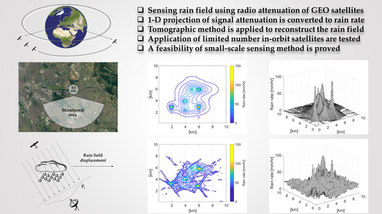
:Sensing of the rain rate and the movement of the rain field over a relatively small geographical area may often be necessary for agricultural purposes, water management objectives or transport management in airports or harbors. In this paper, an entirely passive method is suggested to sense rainfall rate and extension of a rain field, with reconstruction in two dimensions using a tomographic method. In order to achieve this goal, multiple colocated satellite receivers are proposed to measure the beacon signal levels of geostationary satellites received at different azimuth angles. The tomographic reconstruction of the rain field takes the advantage of the dis-placement of the rain field due to the movement of air masses, while the rain intensity along the receiving path is estimated by the attenuation of the radio signal between the satellite and the ground receiver. To realize the proposed system, a complete receiver setup and an existing, operational group of satellites are selected. A widely known rain field modeling method is applied to generate test data and evaluate the system. The feasibility of a technically realizable system is provided, and its capabilities are compared with a hypothetical, ideal system. The methods and algorithms are tested on an existing geographical location, simulating a real operating environment.
1. Introduction
The distribution of rain intensity and the amount of rain fallen over a specific area during a given time is important information and has significance in various application areas. In agriculture, the watering needs of plants depend on the soil moisture, and thus on the previous rain [1]. In city areas, the drainage of precipitation requires a thorough design of the sewer network that can be planned by using long-term statistics and knowledge about the local behavior of rainfall [2]. This is especially important because climate change is significantly influencing the constraints of civil engineering designs. Millimeter-wavelength radio communications systems, like terrestrial point-to-point connections such as the backhaul system of the mobile radios, or satellite-earth connections above 10 GHz, are also suffering from rain attenuation or rain fading [3]. Frequently, the local variations of rainfall statistics significantly change with geographical location, even within a smaller country. Therefore, the precise design of the availability of such radio links requires detailed experience about the local weather conditions and, consequently, available statistical models are less applicable. Last but not least, airports are important examples where rapid rain intensity changes around the runways are particularly interesting in terms of air traffic control.
There are several different methods, techniques, systems and measurement devices to determine the momentary rain intensity over a specific geographical area.
Rain gauges are classical meteorological devices that collect precipitation in the form of liquid water and provide the cumulated rain intensity value for a specific duration, usually for one minute or longer [4]. Disdrometers provide some additional information like drop size distribution, while laser-based sensors or present weather detectors are capable of determining precipitation and visibility parameters as well. However, the devices listed above are the most accurate rainfall intensity sensors. Due to their operation to create a high-resolution rain intensity map of a specific area, many sensors should be installed in a grid-like manner, where the real-time data acquisition of the sensors is also an additional technical problem.
Weather radar systems are complex and usually costly, and consist of a microwave transmitter, receiver and signal-processing unit. Due to the nature of their operation, these active devices detect the reflections of the microwave impulses transmitted, usually in S-band, C-band or X-band and, therefore, they are suitable for remote sensing of the different precipitation types in the range of several cubic kilometers [5]. Weather radar systems are widely used to detect different precipitation field types and visualize their intensity distribution. This is the most common method using an active device to reconstruct the dimensions and displacement direction of the rain field.
A remote sensing method to determine rain intensity based on the measurement of radio wave attenuation between the radio transmitter and receiver was shown for terrestrial point-to-point links in [6] and for satellite connections in [7]. Because of its simplicity to obtain the specific attenuation in dB/km, a well-known power-law expression is applicable as given in recommendation ITU-R P.838 [8]. The specific attenuation depends on the rain rate given in mm/h and on frequency- and polarization-dependent constants. These constants are given in the ITU recommendation for a wide frequency range between 1–1000 GHz. However, their rain rate, temperature and drop size distribution dependency should be taken into account as well [9]. When the attenuation is known (e.g., by measurement) the inverse of the power-law expression is applicable to get the rain rate. For longer radio paths, the rain attenuation is usually not homogenous along the full radio path, thus for calculations the effective path length is applicable. For satellite links, the recommendation ITU-R P.618 [10], and for terrestrial microwave connections the ITU-R P.530 [11] are applicable for the relating calculations.
To visualize a rain field that usually consists of several rain cells with different extensions, accurately measured, or sensed point rain intensity values, are required over the monitored area. Besides the difficult-to-implement grid of rain gauges or applying more costly weather radar systems, in the literature can also be found some remote sensing methods, usually based on radio wave attenuation measurements and tomographic rain field reconstruction principles. The authors in paper [12] compare different rainfall observing techniques in the city of Genoa (Italy): a regional tipping-bucket rain gauge network, the Monte Settepani long-range weather radar, and a network of microwave sensors for satellite downlinks developed by the University of Genoa.
Tomography is based on the idea that the cross-sectional image of an object can be reconstructed from several one-dimensional transmission measurements taken from different angles. Therefore, the tomographic method to reconstruct the rainfall field is not a new idea. As radio waves are attenuated when they are crossing a precipitation area, transmission measurements are feasible by receiving signals from terrestrial or satellite radio sources.
One of the earliest papers dealing with tomographic rain field reconstruction is [13]. A simulation environment was created with a grid of numerous terrestrial millimeter-wavelength radio links over a few hundred square kilometers plane ground area, showing that the spatial distribution of precipitation intensity can be successfully reconstructed with a tomographic method by using the measured path attenuation values. The elements of this system are located in several places; therefore, measured data transfer to a central data processing center has to be also solved.
In [14] tomographic processing was applied using power attenuation measurements on microwave links within the radio base-station networks of a mobile communication systems. A six by six kilometer city area with 89 links was measured and to validate the results the rainfall field was simulated through weather radar data.
The authors of [15] used attenuation measurements over microwave link networks to provide continuous rainfall distribution estimates. A 10 by 10 km area with 33 terrestrial microwave links operating at 12 GHz was utilized for tomographic rain field reconstruction. Compared with radar technology applying longer scans, the proposed method provided real-time imaging.
A tomographic inversion technique is shown in [16] for terrestrial microwave links where the individual radio links operate at different frequencies. An innovative tomographic reconstruction algorithm was proposed that permits dealing with heterogeneous frequency links. Simulations were provided for a 40 by 40 km area with 24 links, and the results were validated with weather radar measurements.
In [17] only three bidirectional K-band terrestrial radio links were applied for attenuation measurements and tomographic rain field reconstruction. The results were compared with the measurement data of nine uniformly arranged rain-gauges over the observation area.
In addition to terrestrial radio links, satellite receivers are also applicable to measure the transmission data and support tomographic techniques for rain field reconstruction. In the literature, tomographic methods for rainfall field reconstruction with low earth orbiting (LEO) and geostationary (GEO) satellites are also described.
The LEO satellites orbit below 2000 km, usually with less than a two hour period. Therefore, to receive their signal and avoid antenna pointing loss, in most cases a tracking system is required on the ground receiver station.
A tomographic rain field reconstruction with LEO satellites was proposed in [18]. This work was based on the power-law relationship between the received attenuated microwave signals on satellite ground stations and the rain intensity. The proposed tomographic reconstruction method used a modified radial basis function model and transformed the reconstruction process into a supervised learning problem. The results were compared with the Global Rainfall Map in Near Real Time product available from the Japan Aerospace Exploration Agency. An improved version of [18] outlined a 3D tomographic rain field reconstruction using the measured LEO received signal level in [19], applying simulations of the satellite trajectory and synthetic rain events to prove the results.
A differential approach was proposed in [20] for tomographic rain field reconstruction using the signal-to-noise ratio of microwave signals from LEO satellites. The unknown baseline values were eliminated to reconstruct the attenuation field by a set of equations that were formed along the movement of the LEO satellites. The reconstruction method and the results were validated by simulations.
Geostationary satellites are placed over the equator, and the observer can see them always in exactly the same spot in the sky. Therefore, no tracking mechanism is required in the ground receiver stations. The radio signal transmitted by a GEO satellite is also applicable to monitor atmospheric events, especially rain fields, by the precipitation-induced attenuation of the radio waves.
There is a limited number of papers dealing with rain field sensing and reconstruction supported by attenuation measurements on the space-Earth radio channel of geostationary satellites. A feasibility study can be found in [21], including some numerical tests of the concept. A slightly improved version of the method can be found in [22]. However, the proposed three-receiver system may significantly influence the quality of reconstruction. In order to apply the tomography method with GEO satellites, it is assumed that during the observation time the rainy area moving across the radio path does not change its internal structure. The authors of [21] and [22] proposed further development of the method, performed simulations, and compared the results with a rain field that was determined with a different measurement technique.
2. Methods
In this article, a small-scale rain field remote sensing method is proposed to observe the rainfall intensity over a relatively small geographical area. The system is fully passive since the principle of operation is based on receiving radio wave transmissions from geostationary satellites. The surface distribution of the rain intensity is reconstructed from the path attenuation measurements by applying a tomographic method. This work was motivated by the fact that in the existing literature a complete system description cannot be found for a real, existing geographical area, taking advantage of local satellite reception conditions. The novelty of this work is that an existing set of geostationary satellites is applied to validate the method, a proven rain cell model is used to simulate a rain field in order to test the quality of the tomographic reconstruction and a feasible system is proposed and tested by simulations within a real geographical location. Furthermore, the impact of the number and position of the observed satellites on the quality of reconstruction is also studied and analyzed, comparing the proposed system with a hypothetical measurement arrangement. The goodness of reconstruction is evaluated by calculating the root mean square and the relative root mean square error by comparing the original rain field with the reconstructed one.
2.1. Location and Observable Satellites
Geostationary satellite orbits are located in the equatorial plane following the Earth’s rotation. There are almost 900 operating geostationary communications satellites [23], more or less evenly distributed on the big circle with a 35,786 km altitude above the surface of the Earth. Depending on the technical parameters of the satellite, such as transmission frequency and power, as well as antenna direction and characteristics, their footprint size and location on the ground surface varies. Therefore, the number of receivable geostationary satellites at a given geographical location is variable. The Ka and Q-band beacon signal coverage map of Alphasat at 25° E [24] is an example of this, providing a coverage over Europe for propagation experiments.
The position of these satellites is defined by their angle of the distance from the prime meridian toward East or West. Therefore, the longitude of the receiver station limits the range of satellites that can be properly received from that place. The latitude of the station relates to the elevation angle set on the receiving antenna. High latitudes produce small elevation angles where the receiving path crosses large air masses. Therefore, the elevated clear-sky attenuation and scintillation level should be taken into account [25]. Scintillation appears as a noise-like superimposed signal over the main received signal. Scintillation can be easily removed from the time series of received signal power by applying a low-pass filter. Therefore, within this technical note this effect is not addressed. At the same time, however, the sampling rate of the receiver must be set fast enough to cope with the evolution of meteorological phenomena meantime. Therefore, in case of a digital system, the sampling rate of the received signal level must be ten samples per minute or even more.
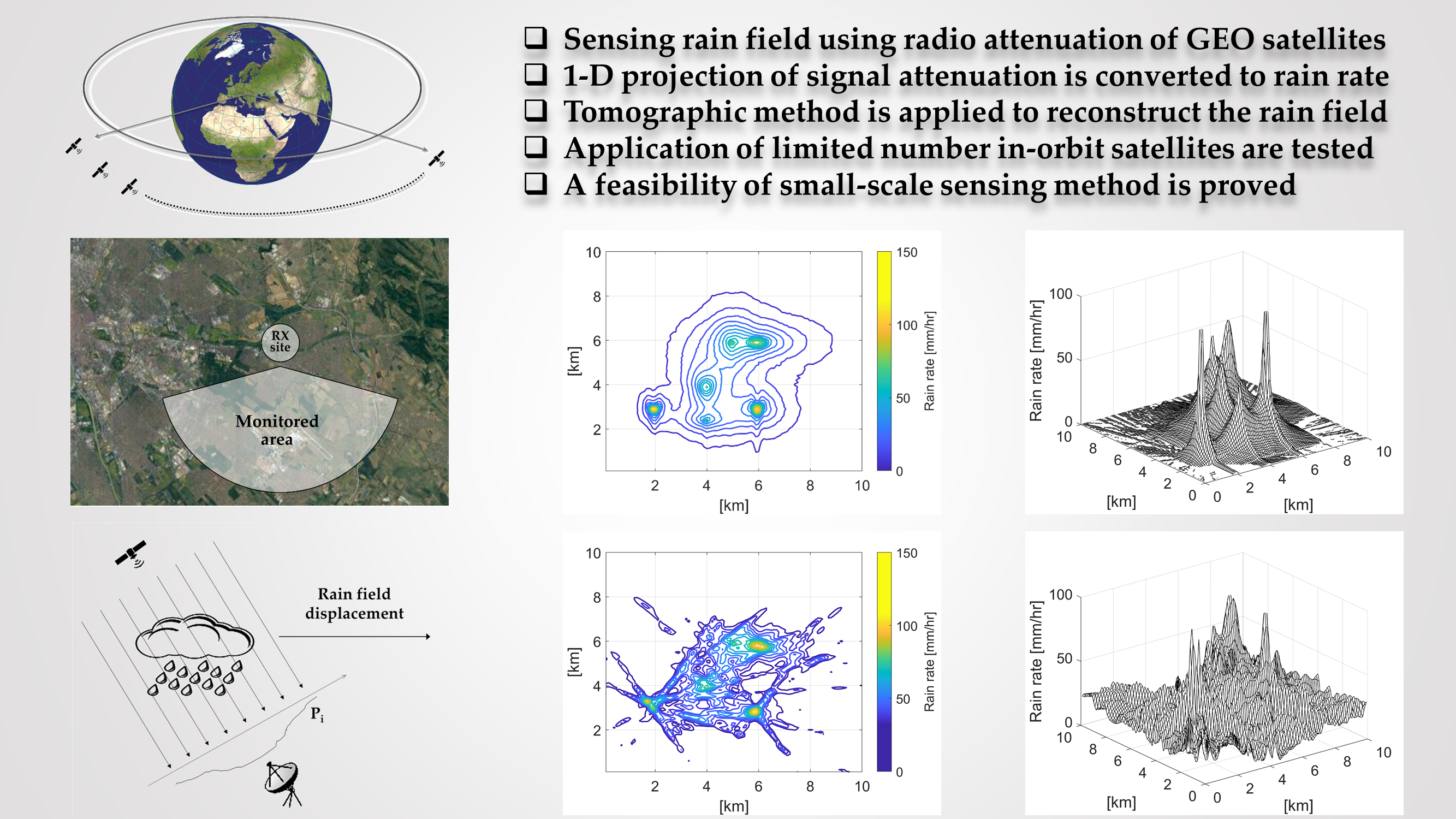
According to practical considerations, mainly related to the size of receiving antennas, geostationary satellites that are located within the range of ±70° of the receiver station’s longitude can be received in satisfactory quality considering the usually wide beam coverage area as well, as is depicted in Figure 1a. To manage the operation of the satellites, and for atmospheric measurements as radio wave propagation studies, the beacon signal of the satellites is applied. A satellite beacon is an unmodulated or low data rate carrier wave transmitted by the satellites to support automatic tracking mechanisms or to determine the exact orbital position of the satellite. For the proposed tomographic rain field reconstruction, the reception of multiple satellite beacon signals is required with a proposed receiver structure as described, for example, in [26].
To demonstrate rain field sensing with path attenuation measurements and two dimensional (2D) tomographic image reconstruction, an existing geographical location was chosen. To perform simulations and validate the results, a location in Budapest was selected, as Figure 1b depicts. The proposed monitoring area of the rain field was the international airport of the city located at 47.43° N latitude and 19.23° E longitude, occupying about a 10 by10 km region. The airport is located 15 km from the city center in a moderately built-up area. The traffic is more than 300 flights a day. Therefore, exact knowledge about the weather conditions is particularly important for air traffic control.
On the geographical location of the receiving site, as shown in Figure 1b, numerous geostationary satellites are receivable. In order to prove the concept and perform the simulations, a proposed list of the satellites with their names, locations, orbit inclination and the highest available beacon frequency bands are listed in Table 1.
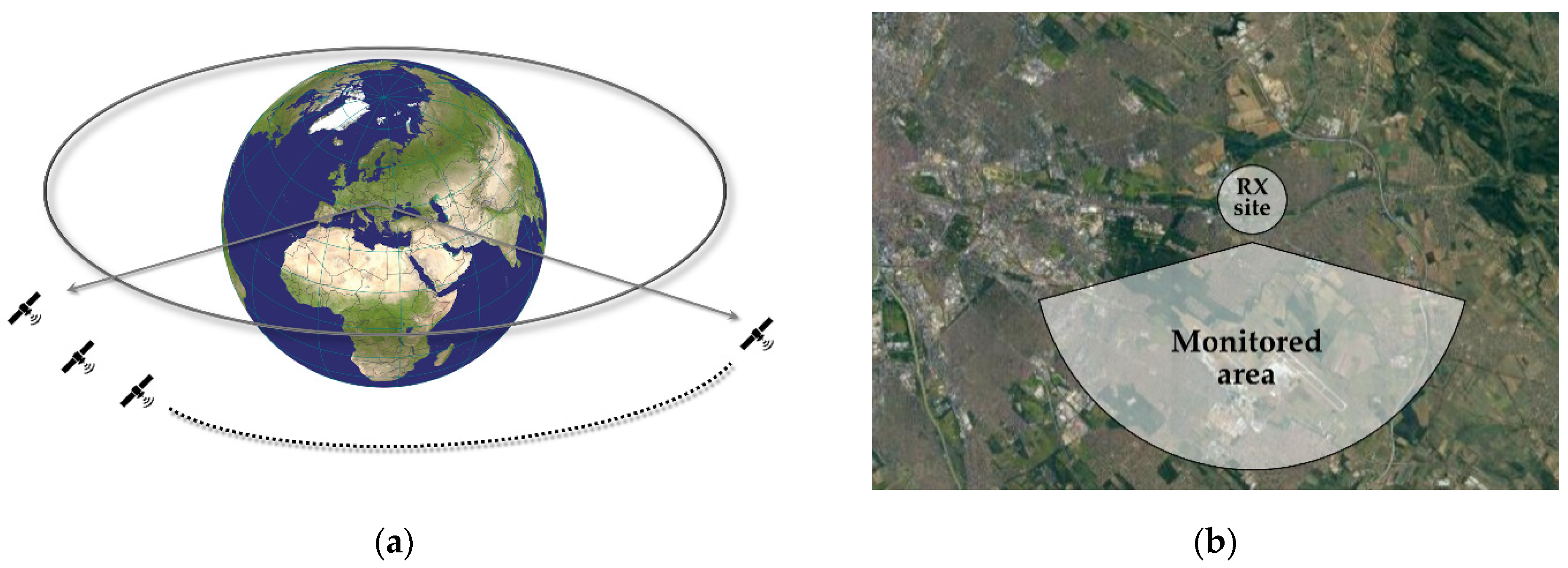
During the selection of the satellites listed in Table 1. it was taken into account that they have active Europe beams, and they are almost evenly distributed on the equatorial plane toward east and west from the Budapest meridian. Figure 2 depicts the azimuth and elevation angles of these satellites.
For practical reasons the two extreme satellites have slightly more than a 15° elevation. In case of very low elevation, the receiving antennas may pick up more ground noise, and atmospheric effects such as attenuation and scintillation, will be much more pronounced. In addition, obstacles (mountains, hills, trees, buildings, etc.) may also block the line-of-sight receiving path. Exclusion of the extremely low elevation receiving antennas only slightly reduces the accuracy of the rain field reconstruction method, but makes installation of large antennas for low-elevation reception unnecessary.
In Table 1, the inclination of the satellite orbits is provided, based on the NORAD Two-Line Element Sets issued on 01 December 2020. It should be highlighted that all of the selected satellites orbit in a geostationary, low inclination orbit (most of them have less than 0.1° inclination). In accordance with international agreements, most geostationary satellites must be kept in a narrow window whose magnitude in geographical longitude and latitude may not exceed ±0.1° [27]. This prevents mutual disturbance of transmission paths and allows controlled usage of the limited space in the geostationary ring. Another large group of GEO satellites are geosynchronous satellites, usually with larger than 1° inclination. The ground received signal level of the geosynchronous satellites may fluctuate because of the nature of the inclined orbit and due to satellite orbit perturbation effects, drift, Doppler frequency shift or satellite maneuvers [27,28]. During the design of a rain-field sensing system based on this Technical Note the selecting of low-inclination, geostationary satellites is highly recommended. In spite of this, a relatively small fluctuation with a 24 h-period is typically present in the received signal even in the case of geostationary satellites, which may be removed, for example, by filtering in the frequency domain. Reception of inclined, geosynchronous satellites results in significant fluctuations in the received signal level [29] and, therefore, a degradation in the reconstruction precision may be observable.
2.2. Rain Field Simulation Method
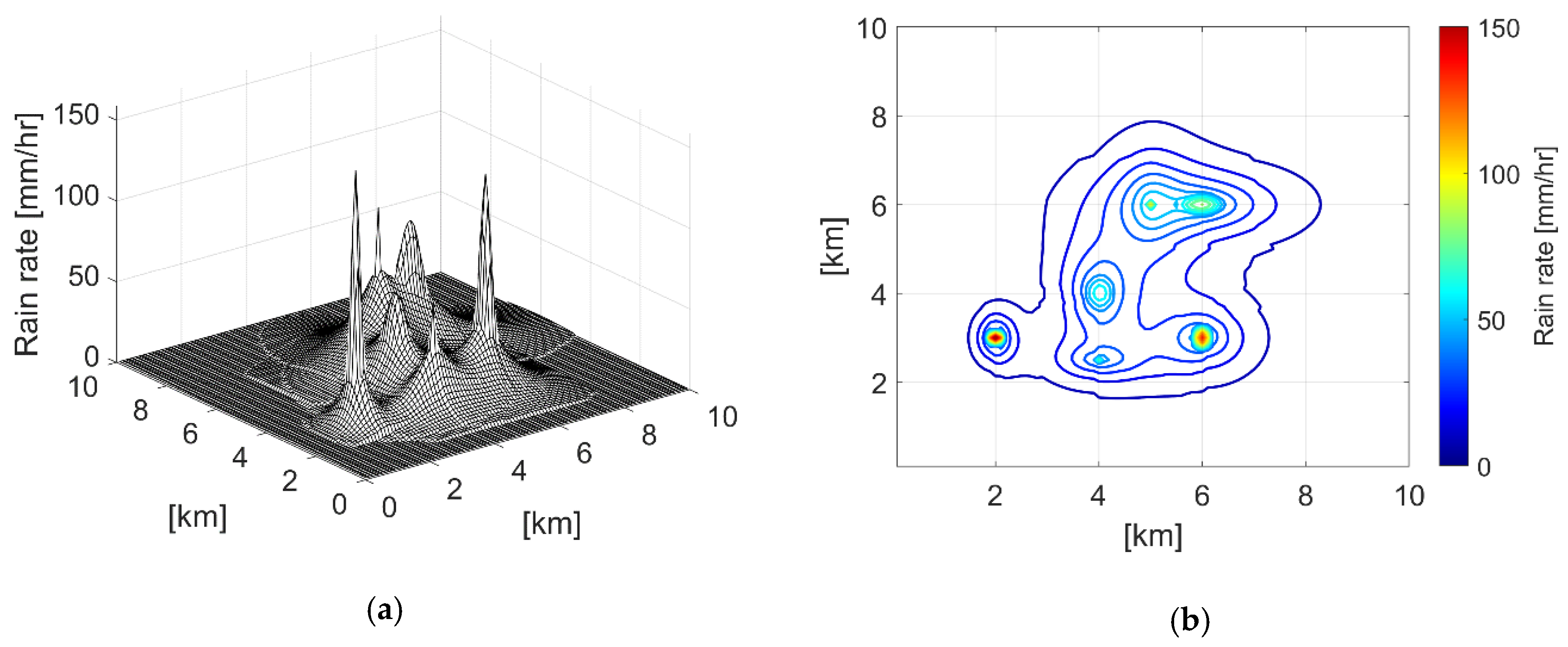
In this paper, the HYCELL model [30] is employed to simulate the individual rain cells in a local rainfall field and test the performance of the tomographic rain field reconstruction method by comparing the original and reconstructed rain fields. The HYCELL model allows statistical representation of the precipitation characteristics of a synthetic isolated cell with rotational symmetry and spatial distribution of the rain intensity. The HYCELL model is an improvement of the EXCELL model [31] by attempting to describe optimally the rain rate horizontal distribution within rain cells having an elliptical or circular horizontal cross-section by combining a Gaussian component with an exponential one. First, the HYCELL model overcomes the problem that exponentially peaked distributions of rain rate are not observed in nature. Second, in the case of high values of the mean rainfall rate, the associated peak rain rate is more realistic than in the case of the EXCELL model. HYCELL is derived from radar observations of rain fields at midlatitudes and it strives to describe optimally the rain rate horizontal distribution within rain cells down to 1 mm/h. A rain field for various scales may be composed of the conglomeration of individual rain cells modelled by HYCELL [30] and [32].
In the HYCELL model for an individual rain cell the analytical expression to calculate the rain rate R(x, y) in a point of the horizontal plane is given in Equation (1) as [30]:
RG, aG, and bG define the Gaussian components the peak rain rate and the distances along the x and y axes on the horizontal plane for which the rain rate decreases by a factor 1/e with respect to RG. RE, aE, and bE define the exponential component with similar signification for the Gaussian component. R1 separates the Gaussian and exponential components, while R2 = 1 mm/h [30] allows to distinguish the rain cell with a significant rain activity from the stratiform shapeless background. The Gaussian component describes the convective-like high rain rate core of the cell, while the exponential component accounts for the surrounding stratiform-like low rain rate.
In this study, considering the small dimensions of the simulation area, a small-scale aggregate of individual cells was generated. The number of cells resulted by using a random generator according to a discrete uniform distribution function, while the distance between two cells could be determined from the nearest neighbor distance distribution as proposed in [33].
In Figure 3 a small-scale, simulated rain field can be seen in a 10 × 10 km area. The individual rain cell parameters were randomized by taking into account real radar observation of a rain cell in Europe, Karlsruhe [33] to limit the peak rain intensity below Rmax = 162 mm/h and the Gaussian components are (aG, bG, aE, bE ) ≤ 1.5 km. For the separation confoustant R1 = 35 mm/h was applied.
2.3. Tomographic Methods for 2D Rain Field Reconstruction
Tomographic methods are applicable to investigate a three-dimensional object with complex internal structure by screening. In the case of absorption tomography, the planar section of a 3D object is screened from different directions, and then the one-dimension records are processed to reconstruct the original planar structure. Johann Radon demonstrated as early as 1917 that a three-dimensional object can be reconstructed from an infinite number of projections. In practical applications, only a finite number of projections are available. Therefore, the reconstruction (back-projection) is always loaded with some errors.
A projection of a two-dimensional function (image) is a set of line integrals. The Radon transform computes these line integrals (often called a sinogram) as 1-D projections from multiple sources along parallel paths in a certain direction. By taking multiple parallel-beam projections in the range of 0–180° by rotating the source around the center of the image, a reconstruction of the original image is possible. If the two-dimensional function is f(x,y), the rotation angle of the projection is Θ, the distance is d from the origin of the image coordinate system, according to [34,35] the line is
and the Radon transform g(d,θ) is expressed with Equation (3):
In this paper, the projections are considered as the path attenuation, measured between a geostationary satellite and the ground receiver station. When the radio path crosses the atmosphere it suffers an attenuation, mainly caused by the integrated precipitation along the path. The magnitude of other attenuating effects like clouds, ice or atmospheric gases (water vapor and oxygen) attenuate to a significantly lesser extent than the rain attenuation.
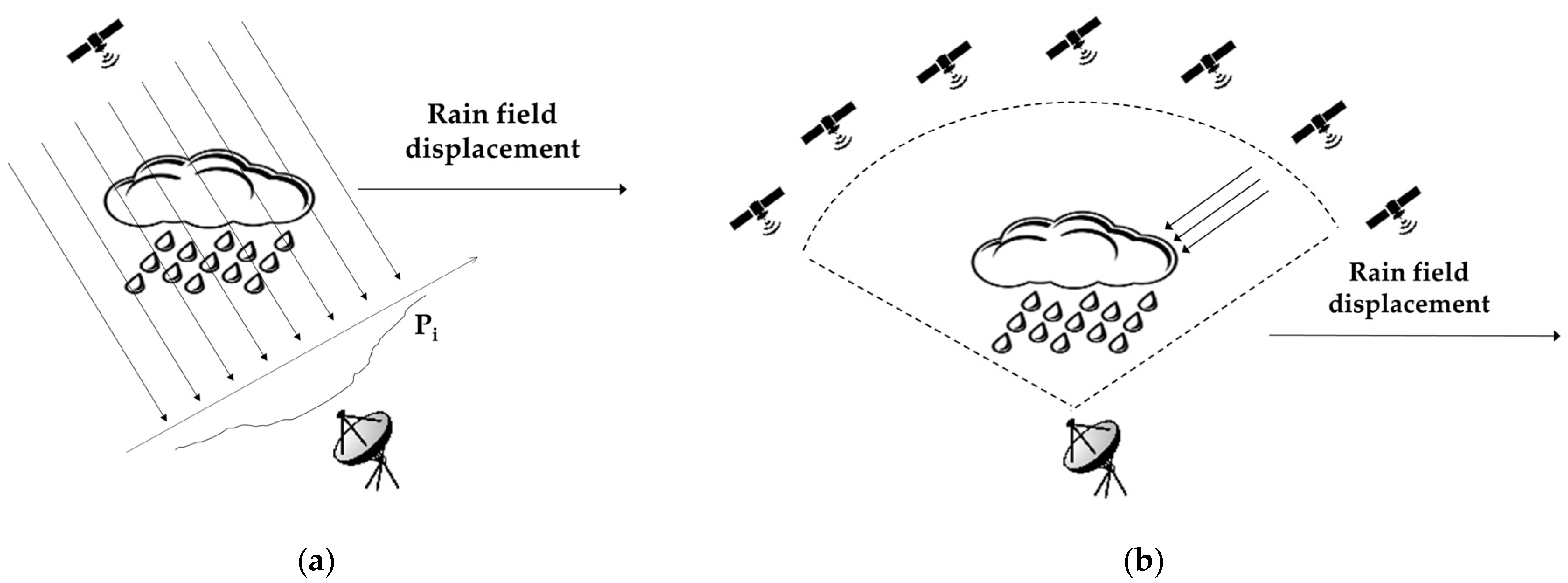
Traditional computer tomography (e.g., for medical application) may apply a single source device and detector linearly translated to record the parallel projections. An analogy of this method is visible in Figure 4a, where the source device is the radio signal of the satellite, while the detector is the receiver station. The source and the detector are fixed in this case, and the displacement is the result of the movement of the rain field. The individual projections of Pi are measured with equidistant Δt timing, determined by the sampling system of the receiver. With the assumption that the rain field displacement direction and speed do not change significantly during recording of the parallel beam projections [22], a set of consistent data can be measured without introducing a distortion in the reconstructed image created during the further processing steps. In this paper, the tomographic reconstruction is proposed for a small-scale use case. Therefore, this assumption is acceptable.
Considering traditional medical tomography again, a rotation of the beam source(s) and the detector(s) is applied to collect an appropriate amount of measurement data and to perform the tomographic image reconstruction. In the case of the proposed rain-field sensing system, the main advantage is that the overall structure of the station is fixed, moving parts are not required. As it can be seen in Figure 4b, the ground receiver station should be prepared to receive multiple geostationary satellites located at different positions above the equator. In the year 2020, according to the UCS Satellite Database, there were more than 500 in-orbit GEO (geosynchronous or geostationary) satellites. As a rule of thumb, the properly receivable GEO satellites are located within ±70° of the receiver station’s longitude. The quality of the received signal is significantly determined by the path length in the atmosphere, which depends on the satellite’s position (usually given in degrees relative to the Greenwich meridian), but the latitude of the receiver should also be taken into account for higher northern or southern longitudes. For the Budapest location to perform the simulations, the set of selected satellites are listed in Table 1.
The measured attenuation on the satellite-Earth path in an analogous way with Equations (2) and (3) is the 1-D projection along the slant path Ls and can be expressed with Equation (4) [9]:
where R(x,y) represents the rainfall rate value interacting with the link at position (x,y), while k and α are frequency and polarization-dependent constants. L0 is the clear-sky attenuation value and must be subtracted from the measured attenuation before the following processing steps. To determine the clear-sky level, one of the most advanced methods is to apply a radiometer [24], but in the proposed system this was not a feasible solution. Based on the former experience in millimeter wavelength propagation measurements [36], to calculate the clear-sky level a simple and cost-effective method is to apply the long-term median of the received signal power for this calculation. A satellite receiver generally records the received signal power, from which the attenuation can be simply obtained by subtracting the current received signal power from the long-term median of the signal power. According to observations on signal power measurements [36], the diurnal variation of the clear-sky level is below ±0.5 dB on a Ka-band (19.701 GHz) channel. Besides this, the fade and interfade duration statistics of a millimeter wavelength radio link [37] provide additional information about the length of the individual fading periods, that influence the long-term median of the received signal power. Based on all considerations a 24 h median value is proposed for the system in question that can be easily determined by the control unit of the multi-satellite receiver system. In the presence of long-lasting (several hours) rain events the evaluated median may lead however to underestimate the reference level. An additional algorithm in the control unit may support exclusion periods with deep attenuation from the median level estimation. When the measured radio wave attenuation is Am, by reversing Equation (4), the estimate of the integrated rain intensity along the path can be determined with Equation (5):
where Le is the effective path length. Because the slant path length LS can be determined as the function of the satellite’s elevation angle and the rain height given in ITU-R P.839 [38], by using ITU’s horizontal and vertical adjustment values the effective path length arises from the slant path length according to ITU-R P.618 [10]. Equation (5) is applicable to reconstruct the rain field by the inverse tomographic method, as is demonstrated in Section 3.
Reconstruction of the investigated object is done by back-projection based on the inverse Radon transformation [39,40]. A common method to perform this is filtered back projection split in two phases, i.e., projection and filtration. In the projection phase, the line integrals are projected back onto the plane at their respective angles [41] using Equation (6):
where f’ is the filtered data. The need for filtering explains that the reconstructed image is heavily blurred. Therefore, a high pass filter is usually applied to the sinogram data in the frequency domain by applying a 1-D DFT (discrete Fourier transform) for each angle, multiplying by the filter, and then using the inverse DFT to reconstruct the data. The number of directions from which parallel projections are taken determines the arrangement of objects that can be distinguished after back-projection. This effect will be discussed Section 3.
2.4. Selecting the Location of the Ground Receiver Station
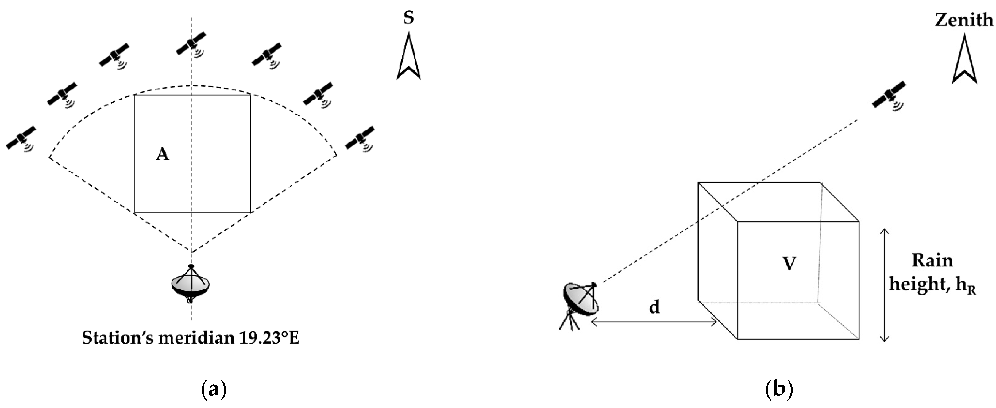
As can be seen in Figure 1b, for Budapest, located in the northern hemisphere, the ground receiver station with the capability of receiving multiple GEO satellites must be to the north of the monitored area. The longitude of the station determines the range of adequately receivable GEO satellites. By taking into account that the monitored area lies on the 19.23° E meridian and the selected satellite positions are symmetrical relative to the monitored area as shown in Table 1, the top view of the scenario is as seen in Figure 5a.
The distance of the station to the north of the monitored area is d as shown in Figure 5b. In the original EXCELL model, the rain cells have a constant vertical rain intensity profile up to the rain height hR, according to ITU-R Rec. P.839 [38,42]. By applying this assumption, the distance d may be estimated with Equation (7):
where Elmax is the highest elevation angle among the received satellites, which for the present case it can be determined from Table 1. The rain height in Budapest is 3.31 km according to ITU-R Rec. P.839 [41], thus d = 4.67 km. This value is applied for the simulations, as will be shown in Section 3.
2.5. Precision of the Proposed Tomographic Reconstruction Method
There are some sources of errors in the proposed remote sensing method, and the tomographic reconstruction process, that slightly influence precision. Nevertheless, the simulations as presented in Section 3 are encouraging. One shortcoming of the presented method is that the signal passes through the melting layer, which can be effectively considered as an extension of the link path in rain. This leads to higher rainfall estimates [43]. Taking advantage of the relatively thin property of the melting layer (<500 m) [44,45] and considering the fact that the beacon signal frequencies of the selected satellites are located in the Ku-band or below, this problem area is not investigated in this paper. The proposed rain field sensing and reconstruction method serves, first of all, for a simple and rough estimate of the local rainfall intensity, and since the major attenuation source is the rain, it does not distinguish the different attenuation sources.
It should be emphasized, also, that the rain height depends on the height of the zero-degree isotherm, and its value influences the effective path length Le whose value is applied in Equation (5). The zero-degree isotherm has seasonal variations, as it is given for a 35-year period in Florence, Italy [46], and it shows an easily observable periodicity. Contrarily, the ITU-R Rec. P.839 [38] provides only an average zero-degree isotherm value for a specific geographical location. Based on the study published in [46], the zero-degree isotherm height exhibits a roughly ±45% yearly variation. After performing calculations supported by recommendation ITU-R P.618 [10], the variation of the effective path length is predictable. Consequently, the rain rate computed with Equation (5) for Budapest location at 12 GHz frequency varies by ±19%. It is difficult to measure the momentary value of the zero-degree isotherm, and it is not possible by the simple, passive receiver structure that is proposed in this paper. However, based on the findings in [46], an algorithm could be implemented in the receiver system that resolves this problem by applying a compensation algorithm taking the advantage of the periodicity of the zero-degree isotherm height.
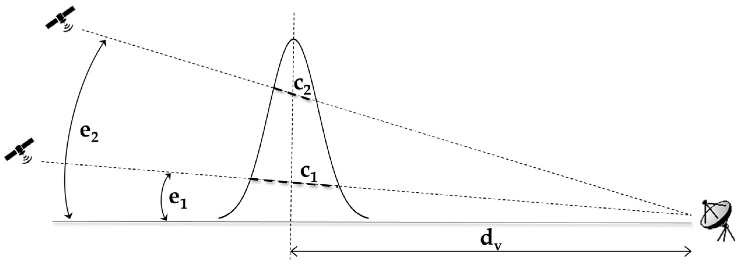
The number of projection angles influences the quality of the reconstruction [47]. Selecting a feasible number of received satellites may lead to an optimal solution considering the cost and complexity of the receiver system against the required reconstruction quality. The impossibility of receiving GEO satellites with a very low elevation angle narrows the optimal 0–180° projection range [48]. In this paper, for the simulations and rain field reconstruction, the width of this range is 144.2°. In traditional tomographic methods all projections are created on the same plane. The present method, by receiving GEO satellites, does not meet this condition, considering the variable elevation angle of the received satellites, as depicted in Figure 6.
When the distance between the receiver station and the rain cell’s vertical axis is dv, the height difference hd of the cross sections’ center points is expressed by Equation (8).
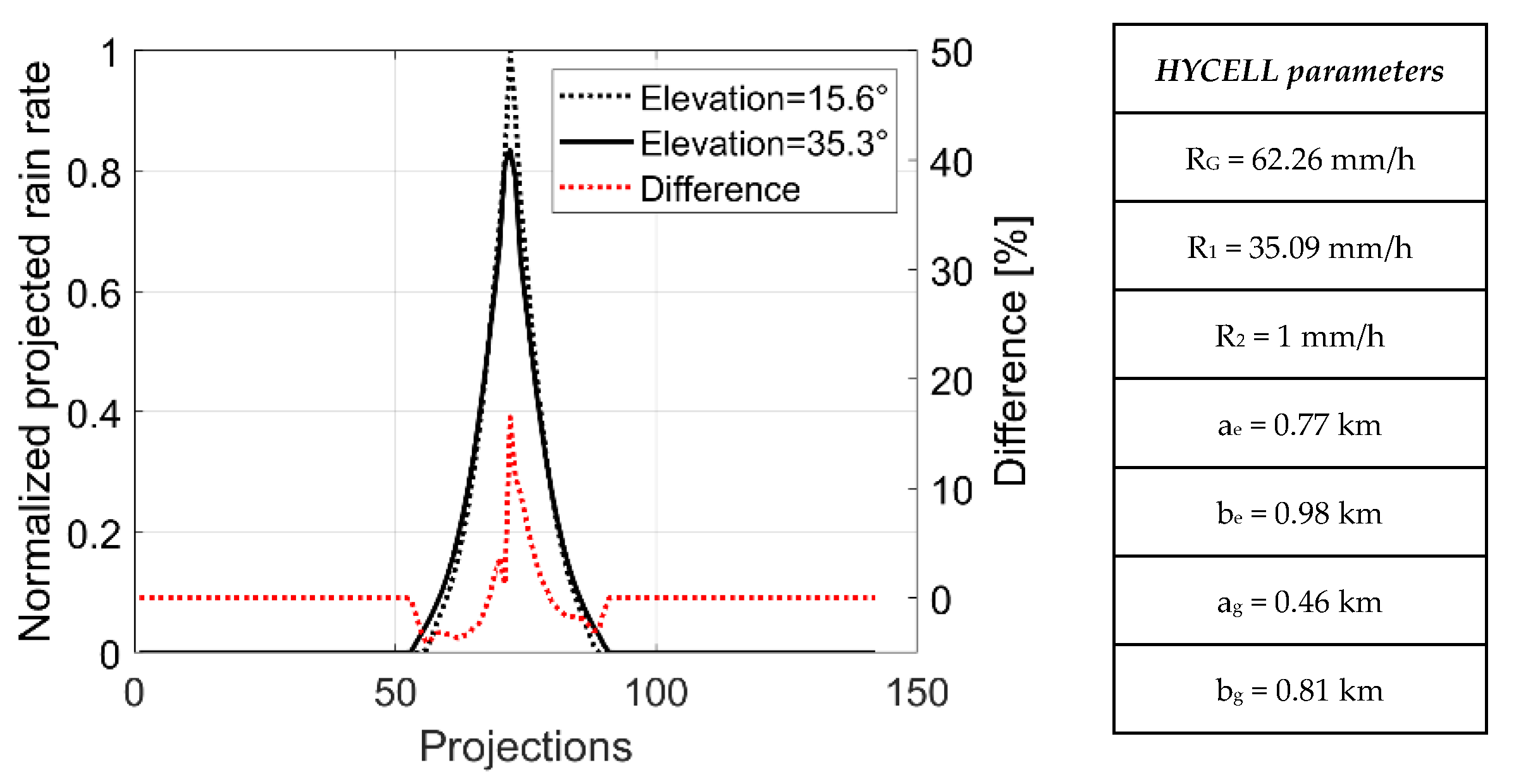
The HYCELL model predicts the decrease of the rain rate from the center of the rain cell according to an exponential or Gaussian curve depending on the separation constant, as given in Equation (1). The high elevation satellite links cross the Gaussian cell structure, while the low elevation links cross the exponential one. The projections from x1 ≤ x ≤ x2 provide the cumulated rain intensity RC along the satellite-receiver path given by the integral of Equation (1), considering that the argument y = y0 is constant:
By solving numerically Equation (9), RC can be calculated. For a typical rain cell, Figure 7 depicts the projected rain intensities for the lowest and highest elevations as given in Table 1, considering the proposed simulation scenario:
The deviation of the integrated rain intensities of the lowest and highest elevations is less than ten percent 94% of the time. Therefore, the projection error caused by receiving satellites with different elevation angles is ignored during the simulations.
3. Simulation Results
Recording Parallel Projections of the Rain Field
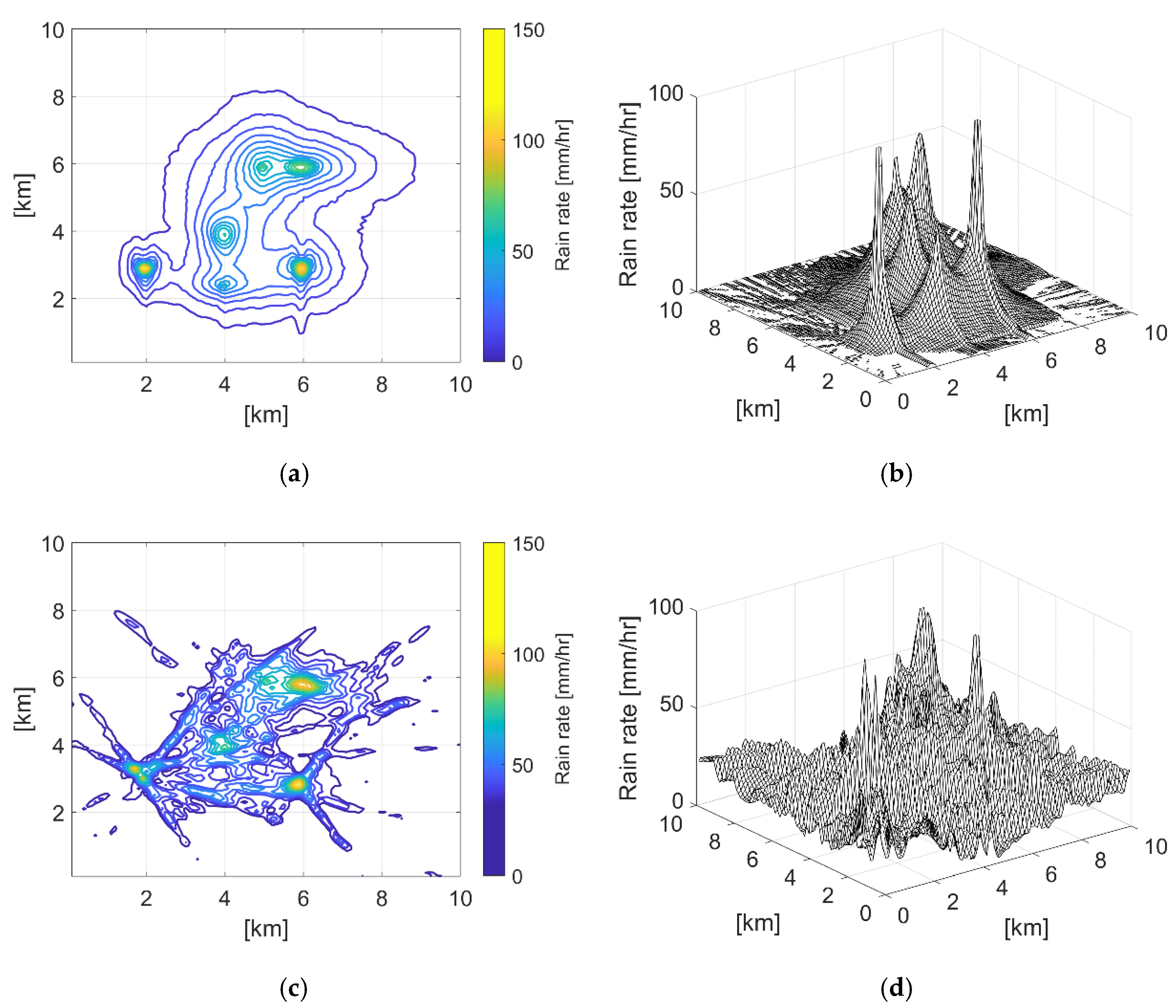
In Figure 4a, the parallel projection method is outlined, implemented by a satellite receiving system. The beacon signal transmitted by the satellite serves as a beam source, while the linear movement of the detector is represented by the displacement of the rain field. In order to prove the capability of the tomographic rain field reconstruction method, Figure 8a was created. A hypothetical satellite receiving system was applied for this simulation, where the HYCELL modelled rain field shown in Figure 3a and b is sensed by 180 GEO satellites equally spaced above the equator, showing a ±90° range of azimuth at the station location relative to the southern direction. The elevations of the hypothetical satellites increase evenly between 0° and 35°, then decrease steadily from 35° to 0°.
The RMSE (Root Mean Square Error) of the reconstruction is 2.97 mm/h for Figure 8a, calculated as the element-wise difference of the original rain field I0 and the reconstructed rain field IR using Equation (10) as the quadratic mean of the differences [49]. The RRMSE (Relative Root Mean Square Error) is 0.418, and was calculated by dividing RMSE by the mean of the original rain field data using Equation (11) [49]:
The locations of the individual rain cells and the cell contours are managed to reconstruct well, including also the rain intensity values. Figure 8b depicts the 3D view of the reconstructed rain field.
An extremely high number of received satellite signals is not feasible for a real system. Therefore, to prove the concept of using a lower number of satellite beams for sensing and reconstruction, the satellite configuration as listed in Table 1 was tested. The result of the rain field reconstruction can be seen in Figure 8c, while the 3D view of the reconstructed rain field is shown in Figure 8d. The RMS reconstruction error is 20.56 mm/h, while RRMSE = 2.89. In the figure, the structure of the projection lines is observable, and the reconstructed rain intensity is slightly elevated around the rain cells.
The relating literature proposes different methods to improve the quality of the restoration. As the number of projection lines is limited in the present case, restoration of data may be applied, as was published in [47]. A compensation method for incomplete sinogram data can be found in [48]. However, in this work no postprocessing of the results was applied, as the intention was to demonstrate the native performance of the proposed system. A further improvement of the final result may be achieved by applying the above-mentioned compensation methods.
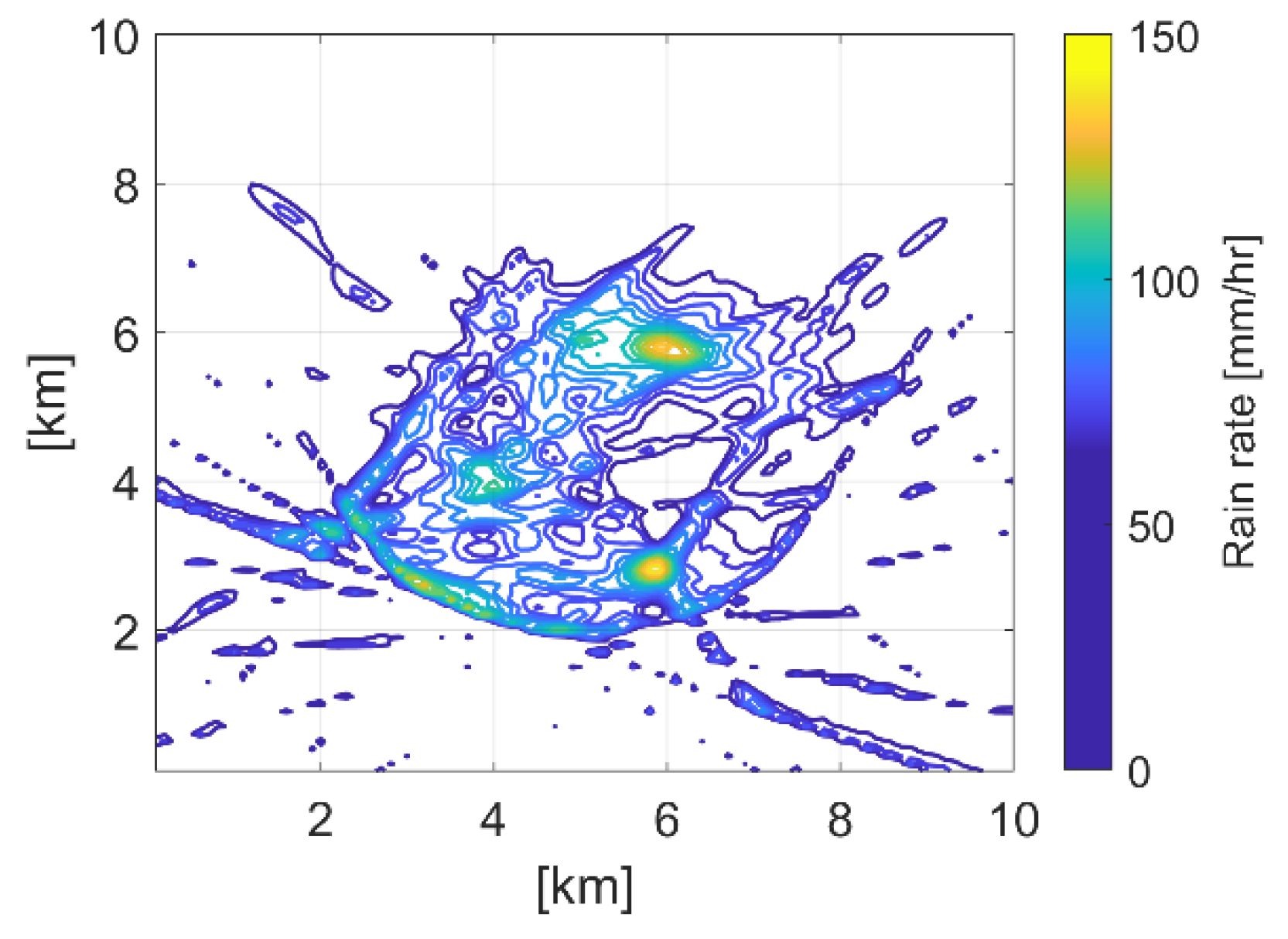
The simulations presented in Figure 8 were created by considering a complete movement of the rain field in front of the receiver station, allowing recording of all parallel projections across the rain field from each satellite elevation. However, to reconstruct the rain field, an entire displacement is not required, as it can be seen in Figure 9. The rain field was simulated to move only by 80% of its total width. The locations of the individual rain cells were not changed in the reconstructed image, but an increased RMS error of 52.33 mm/h and RRMSE = 7.36 was observed.
4. Conclusions
In this paper, a complete and feasible system is outlined for small-scale rain field remote sensing with only passive devices receiving GEO satellite signals and reconstructing the rain field by tomographic methods. The sensing area was a few square kilometers; thus the method is applicable to observe local geographical regions. Existing in-orbit satellites are proposed to implement the method, and the selection of the satellites and the calculation of the exact receiver site location relative to the monitoring area are provided. To prove the concept, the well-known HYCELL model was applied to model the individual rain cells, while the small-scale rain field was modeled as a conglomeration of the individual cells. The quality of the rain field reconstruction was analyzed, the limitation of the measurement structure was shown, and the improvement possibilities were highlighted. The proposed method and the remote sensing system are based on simple technical construction and a low maintenance cost is expected. Thus, it is recommended that remote sensing systems be used to observe rain activity over a small-scale area. Many applications of the proposed method are conceivable, especially where the goal is to observe local precipitation conditions. Taking into account the structure of the proposed system, it is sufficient to install it in a properly selected location. Therefore, there is no need for external sensors. In order to improve the accuracy of the proposed system, in the future a compensation algorithm could be implemented that resolves the problem of the periodic variation of the zero-degree isotherm height. Hopefully the proposed system will be implemented soon and tested under real conditions.
Funding
The research reported in this paper and carried out at the Budapest University of Technology and Economics was supported by the National Research Development and Innovation Fund based on the charter of bolster issued by the National Research Development and Innovation Office under the auspices of the Ministry for Innovation and Technology.
Acknowledgments
This research was inspired by the Alphasat Aldo Paraboni scientific and communication experiment.
Conflicts of Interest
The authors declare no conflict of interest. The funders had no role in the design of the study; in the collection, analyses, or interpretation of data; in the writing of the manuscript, or in the decision to publish the results.
References
- Torres, M.; Howitt, R.E.; Rodrigues, L.N. Analyzing rainfall effects on agricultural income: Why timing matters. Economica 2019, 20, 1–14. [Google Scholar] [CrossRef]
- Cook, L.M.; Vanbriesen, J.M.; Samaras, C. Using rainfall measures to evaluate hydrologic performance of green infrastructure systems under climate change. Sustain. Resilient Infrastruct. 2019. [Google Scholar] [CrossRef] [Green Version]
- Hilt, A. Availability and fade margin calculations for 5G microwave and millimeter-wave anyhaul links. Appl. Sci. 2019, 9, 5240. [Google Scholar] [CrossRef] [Green Version]
- Rodda, J.C.; Dixon, H. Rainfall measurement revisited. Weather 2012, 67, 131–136. [Google Scholar] [CrossRef] [Green Version]
- Yeary, M.; Cheong, B.L.; Kurdzo, J.M.; Yu, T.; Palmer, R. A brief overview of weather radar technologies and instrumentation. IEEE Instrum. Meas. Mag. 2014, 17, 10–15. [Google Scholar]
- Goldshtein, O.; Messer, H.; Zinevich, A. Rain rate estimation using measurements from commercial telecommunications links. IEEE Trans. Signal Process. 2009, 57, 1616–1625. [Google Scholar] [CrossRef]
- Giannetti, F.; Reggiannini, R.; Moretti, M.; Adirosi, E.; Baldini, L.; Facheris, L.; Antonini, A.; Melani, S.; Bacci, G.; Petrolino, A.; et al. Real-time rain rate evaluation via satellite downlink signal attenuation measurement. Sensors 2017, 17, 1864. [Google Scholar] [CrossRef]
- ITU. Recommendation ITU-R P.838-3. Specific Attenuation Model for Rain for Use in Prediction Methods; ITU: Geneva, Switzerland, 2005. [Google Scholar]
- Olsen, R.; Rogers, D.; Hodge, D. The aRb relation in the calculation of rain attenuation. IEEE Trans. Antennas Propag. 1978, 26, 318–329. [Google Scholar] [CrossRef]
- ITU. Recommendation ITU-R P.618-13. Propagation Data and Prediction Methods Required for the Design of Earth-Space Telecommunication Systems; ITU: Geneva, Switzerland, 2017. [Google Scholar]
- ITU. Recommendation ITU-R P.530-17. Propagation Data and Prediction Methods Required for the Design of Terrestrial Line-of-Sight Systems; ITU: Geneva, Switzerland, 2017. [Google Scholar]
- Colli, M.; Cassola, F.; Martina, F.; Trovatore, E.; Delucchi, A.; Maggiolo, S.; Caviglia, D.D. Rainfall fields monitoring based on satellite microwave down-links and traditional techniques in the city of Genoa. IEEE Trans. Geosci. Remote Sens. 2020, 58, 6266–6280. [Google Scholar] [CrossRef]
- Giuli, D.; Toccafondi, A.; Gentili, G.B.; Freni, A. Tomographic reconstruction of rainfall fields through microwave attenuation measurements. J. Appl. Meteorol. 1991, 30, 1323–1340. [Google Scholar]
- Cuccoli, F.; Facheris, L.; Gori, S. Radio base network and tomographic processing for real time estimation of the rainfall rate fields. In Proceedings of the IEEE International Geoscience and Remote Sensing Symposium, Cape Town, South Africa, 12–17 July 2009. [Google Scholar]
- Cuccoli, F.; Facheris, L. Rainfall monitoring based on microwave link attenuation and related tomographic processing. In Proceedings of the Tyrrhenian Workshop on Advances in Radar and Remote Sensing (TyWRRS), Naples, Italy, 12–14 September 2012; pp. 172–176. [Google Scholar]
- D’Amico, M.; Cerea, L.; de Michele, C.; Nebuloni, R.; Cubaiu, M. Tomographic reconstruction of rainfall fields using heterogeneous frequency microwave links. In Proceedings of the IEEE Statistical Signal Processing Workshop (SSP), Freiburg, Germany, 10–13 June 2018; pp. 125–129. [Google Scholar]
- D’Amico, M.; Manzoni, A.; Solazzi, G.L. Use of operational microwave link measurements for the tomographic reconstruction of 2-D maps of accumulated rainfall. IEEE Geosci. Remote Sens. Lett. 2016, 13, 1827–1831. [Google Scholar] [CrossRef]
- Xu, L.; Shen, X.; Huang, D.D.; Feng, X.; Wang, W. Tomographic reconstruction of rainfall fields using satellite communication links. In Proceedings of the 23rd Asia-Pacific Conference on Communications (APCC), Perth, Australia, 11–13 December 2017; pp. 1–5. [Google Scholar]
- Shen, X.; Huang, D.D.; Song, B.; Vincent, C.; Togneri, R. 3-D tomographic reconstruction of rain field using microwave signals from LEO satellites: Principle and simulation results. IEEE Trans. Geosci. Remote Sens. 2019, 57, 5434–5446. [Google Scholar] [CrossRef]
- Shen, X.; Huang, D.; Vincent, C.; Wang, W.; Togneri, R. A differential approach for rain field tomographic reconstruction using microwave signals from Leo satellites. In Proceedings of the IEEE International Conference on Acoustics, Speech and Signal Processing (ICASSP), Barcelona, Spain, 4–8 May 2020; pp. 9001–9005. [Google Scholar]
- Fujita, M. Two-dimensional rain mapping using transmissions from geostationary satellites. In Proceedings of the IEEE International Geoscience and Remote Sensing Symposium (Cat. No. 01CH37217), Sydney, Australia, 9–13 July 2001; pp. 1041–1043. [Google Scholar]
- Fujita, M.; Kurakawa, H.; Suzuki, H. Tomographic rain measurement system using transmissions from geostationary satellites. In Proceedings of the ISAP’04, Sendai, Japan, 17–21 August 2004. [Google Scholar]
- Satbeams. List of Satellites at Geostationary Orbit. Available online: https://www.satbeams.com/satellites (accessed on 1 December 2020).
- Codispoti, G.; Parca, G.; Ruggieri, M.; Rossi, T.; de Sanctis, M.; Riva, C.; Luini, L. The role of the Italian Space Agency in investigating high frequencies for satellite communications: The Alphasat experiment. Int. J. Satell. Commun. Netw. 2019, 37, 387–396. [Google Scholar] [CrossRef]
- Nessel, J.; Boulanger, X.; Castanet, L.; Prytz, T.; Martellucci, A. Results from one year of Ka-band beacon measurements at Svalbard. In Proceedings of the 24th Ka and Broadband Communications Conference and 36th International Communications Satellite Systems Conference, ICSSC 2018, Niagara Falls, ON, Canada, 15–18 October 2018. [Google Scholar]
- Machado, F.; Vilar, E.; Perez-Fontan, F.; Pastoriza-Santos, V.; Marino, P. Easy-to-build satellite beacon receiver for propagation experimentation at millimeter bands. Radioengineering 2014, 23, 154–164. [Google Scholar]
- Ley, W.; Wittmann, K.; Hallmann, W. (Eds.) Handbook of Space Technology; John Wiley & Sons, Ltd.: Hoboken, NJ, USA, 2011. [Google Scholar]
- Maral, G.; Bousquet, M.; Sun, Z. Satellite Communications Systems: Systems, Techniques and Technology, 6th ed.; John Wiley & Sons, Ltd.: Hoboken, NJ, USA, 2020. [Google Scholar]
- Gharanjik, A.; Shankar, M.R.B.; Zimmer, F.; Ottersten, B. Centralized rainfall estimation using carrier to noise of satellite communication links. IEEE J. Sel. Areas Commun. 2018, 36, 1065–1073. [Google Scholar]
- Féral, L.; Sauvageot, H.; Castanet, L.; Lemorton, J. HYCELL—A new hybrid model of the rain horizontal distribution for propagation studies: 1. Modeling of the rain cell. Radio Sci. 2003, 38. [Google Scholar] [CrossRef] [Green Version]
- Capsoni, C.; Fedi, F.; Magistroni, C.; Paraboni, A.; Pawlina, A. Data and theory for a new model of the horizontal structure of rain cells for propagation applications. Radio Sci. 1987, 22, 395–404. [Google Scholar]
- Féral, L.; Sauvageot, H.; Castanet, L.; Lemorton, J. HYCELL—A new hybrid model of the rain horizontal distribution for propagation studies: Part 2, Statistical modeling of the rain rate field. Radio Sci. 2003, 38. [Google Scholar] [CrossRef]
- Castanet, L. (Ed.) Influence of the Variability of the Propagation Channel on Mobile, Fixed Multimedia and Optical Satellite Communications; Shaker Publishing: Düren, Germany, 2008. [Google Scholar]
- France, A.; CEA Saclay. The Radon Transform and Its Inverse; Technical Report; CEA Saclay: Paris, France, August 2011. [Google Scholar]
- Akeza, A.; Chakraborty, S.; Hari, N.; Man, R.; Bhattacharya, C. Comparative analysis of three different algorithms for radon transform. In Proceedings of the International Conference on MetaComputing (ICoMeC), Goa, India, 15–16 December 2011. [Google Scholar]
- Csurgai-Horváth, L.; Adjei-Frimpong, B.; Riva, C.; Luini, L. Radio wave satellite propagation in Ka/Q band. Period. Polytech. Electr. Eng. Comput. Sci. 2018, 62, 38–46. [Google Scholar] [CrossRef] [Green Version]
- Pimienta-del-Valle, D.; Riera, J.M.; Garcia-del-Pino, P.; Siles, G.A. Three year fade and inter fade duration statistics from the Q-band Alphasat propagation experiment in Madrid. Int. J. Satell. Commun. Netw. 2019, 37, 460–476. [Google Scholar] [CrossRef]
- ITU. Recommendation ITU-R P.839-4. Rain Height Model for Prediction Methods; ITU: Geneva, Switzerland, 2013. [Google Scholar]
- Deans, S.R. The Radon Transform and Some of Its Applications; Krieger Publishing Company: Malabar, FL, USA, 1992. [Google Scholar]
- Viergever, M.; Todd-Pokropek, A. (Eds.) Mathematics and Computer Science in Medical Imaging; Springer: Berlin, Germany, 1988. [Google Scholar]
- Toft, P. The radon Transform. Theory and Implementation. Ph.D. Thesis, Danmarks Tekniske University, Institute for Matematisk Modellering, Lyngby, Denmark, November 1996. [Google Scholar]
- Riasol, R.P. SC-EXCELL Model Upgrade to Predict Depolarization. Bachelor’s Thesis, Universitat Politecnica de Catalunya Barcelonatech, Barcelona, Spain, May 2014. [Google Scholar]
- Arslan, C.H.; Aydin, K.; Urbina, J.V.; Dyrud, L. Satellite-link attenuation measurement technique for estimating rainfall accumulation. IEEE Trans. Geosci. Remote Sens. 2018, 56, 681–693. [Google Scholar] [CrossRef]
- Matrosov, S.Y. Assessment of radar signal attenuation caused by the melting hydrometeor layer. IEEE Trans. Geosci. Remote Sens. 2008, 46, 1039–1047. [Google Scholar] [CrossRef]
- Wolfensberger, D.; Scipion, D.; Berne, A. Detection and characterization of the melting layer based on polarimetric radar scans. Q. J. R. Meteorol. Soc. 2016, 142, 108–124. [Google Scholar] [CrossRef]
- Adirosi, E.; Facheris, L.; Petrolino, A.; Giannetti, F.; Reggiannini, R.; Moretti, M.; Scarfone, S.; Melani, S.; Collard, F.; Bacci, G. Exploiting satellite Ka and Ku links for the real-time estimation of rain intensity. In Proceedings of the 2017 XXXII General Assembly and Scientific Symposium of the International Union of Radio Science (URSI GASS), Montreal, QC, Canada, 19–26 August 2017. [Google Scholar]
- Huang, Y.; Huang, X.; Taubmann, O.; Xia, Y.; Haase, V.; Hornegger, J.; Lauritsch, G.; Maier, A. Restoration of missing data in limited angle tomography based on Helgason-Ludwig consistency conditions. Biomed. Phys. Eng. Express 2017, 3. [Google Scholar] [CrossRef]
- Happonen, A. Decomposition of Radon Projections into Stackgrams for Filtering, Extrapolation, and Alignment of Sinogram Data. Ph.D. Thesis, Tampere University of Technology, Tampere, Finland, November 2005. [Google Scholar]
- Kenney, J.F.; Keeping, E.S. Mathematics of Statistics, 3rd ed.; Princeton: Princeton, NJ, USA, 1962. [Google Scholar]
Figure 1.
(a) Satellite receiving range: about 140°; (b) The simulation area: city of Budapest with the ground receiver station and the public airport as the monitored area.
Figure 1.
(a) Satellite receiving range: about 140°; (b) The simulation area: city of Budapest with the ground receiver station and the public airport as the monitored area.

Figure 2.
Azimuth and elevation angles of the satellites listed in Table 1. As seen from Budapest.
Figure 2.
Azimuth and elevation angles of the satellites listed in Table 1. As seen from Budapest.

Figure 3.
(a) 3D plot of a small-scale simulated rain field using the HYCELL model; (b) Contour plot of the rain field.
Figure 3.
(a) 3D plot of a small-scale simulated rain field using the HYCELL model; (b) Contour plot of the rain field.

Figure 4.
(a) Parallel-beam projections of the rain field, recording during displacement; (b) recording multiple parallel-beam projections by receiving multiple geostationary satellites.
Figure 4.
(a) Parallel-beam projections of the rain field, recording during displacement; (b) recording multiple parallel-beam projections by receiving multiple geostationary satellites.

Figure 5.
(a) Top view of the monitored area A; (b) distance d of the receiver station from the monitored volume V.
Figure 5.
(a) Top view of the monitored area A; (b) distance d of the receiver station from the monitored volume V.

Figure 6.
Cross-sections of the rain cell (c1, c2) when satellites are received with different elevation angles e1 and e2.
Figure 6.
Cross-sections of the rain cell (c1, c2) when satellites are received with different elevation angles e1 and e2.

Figure 7.
Rain intensity projection values for the lowest and the highest elevation angles calculated with Equation (9) for a single rain cell with the given parameters.
Figure 7.
Rain intensity projection values for the lowest and the highest elevation angles calculated with Equation (9) for a single rain cell with the given parameters.

Figure 8.
(a) Tomographic reconstruction of the original rain field by a hypothetical receiving system using 180 equally arranged satellites; (b) 3D view of the rain field; (c) reconstruction based on satellite constellation provided in Table 1; (d) 3D view of the rain field.
Figure 8.
(a) Tomographic reconstruction of the original rain field by a hypothetical receiving system using 180 equally arranged satellites; (b) 3D view of the rain field; (c) reconstruction based on satellite constellation provided in Table 1; (d) 3D view of the rain field.

Figure 9.
Reconstruction after partial displacement of the rain field.


Table 1.
Parameters of satellites selected for the simulations. Azimuth and elevation degrees are calculated for Budapest, 96 m above sea level.
Table 1.
Parameters of satellites selected for the simulations. Azimuth and elevation degrees are calculated for Budapest, 96 m above sea level.
| Name | Location | Inclination | Highest Beacon Frequency | Azimuth | Elevation |
|---|---|---|---|---|---|
| HISPASAT-30W | 31.5W | 0.073° | X-band | 240.6° | 15.8° |
| INTELSAT-907 | 27.5W | 0.578° | X-band | 235.1° | 19.4° |
| TELSTAR-12 | 15W | 0.017° | X-band | 222.5° | 26.2° |
| EUTELSAT 5 WEST A | 5W | 0.954° | Ku-band | 211.2° | 30.6° |
| EUTELSAT 7B | 7E | 0.066° | X-band | 196.2° | 34.1° |
| EUTELSAT 16A | 16E | 0.067° | Ku-band | 184.2° | 35.3° |
| ASTRA 2F | 28.2E | 0.080° | X-band | 167.8° | 34.7° |
| EUTELSAT-36B | 36E | 0.067° | X-band | 157.6° | 33° |
| INTELSAT-38 | 45E | 0.027° | X-band | 146.7° | 29.9° |
| INTELSAT-33e | 60E | 0.039° | C-band | 130.4° | 22.7° |
| INTELSAT-20 | 68.5E | 0.013° | Ku-band | 122.3° | 17.8° |
| INTELSAT-22 | 72.1E | 0.002° | C-band | 119.1° | 15.6° |
Publisher’s Note: MDPI stays neutral with regard to jurisdictional claims in published maps and institutional affiliations. |
© 2020 by the author. Licensee MDPI, Basel, Switzerland. This article is an open access article distributed under the terms and conditions of the Creative Commons Attribution (CC BY) license (http://creativecommons.org/licenses/by/4.0/).
Share and Cite
MDPI and ACS Style
Csurgai-Horváth, L. Small Scale Rain Field Sensing and Tomographic Reconstruction with Passive Geostationary Satellite Receivers. Remote Sens. 2020, 12, 4161. https://0-doi-org.brum.beds.ac.uk/10.3390/rs12244161
AMA Style
Csurgai-Horváth L. Small Scale Rain Field Sensing and Tomographic Reconstruction with Passive Geostationary Satellite Receivers. Remote Sensing. 2020; 12(24):4161. https://0-doi-org.brum.beds.ac.uk/10.3390/rs12244161
Chicago/Turabian StyleCsurgai-Horváth, László. 2020. "Small Scale Rain Field Sensing and Tomographic Reconstruction with Passive Geostationary Satellite Receivers" Remote Sensing 12, no. 24: 4161. https://0-doi-org.brum.beds.ac.uk/10.3390/rs12244161
Note that from the first issue of 2016, this journal uses article numbers instead of page numbers. See further details here.