The Role of Improved Ground Positioning and Forest Structural Complexity When Performing Forest Inventory Using Airborne Laser Scanning

Abstract

The level of spatial co-registration between airborne laser scanning (ALS) and ground data can determine the goodness of the statistical inference used in forest inventories. The importance of positioning methods in the field can increase, depending on the structural complexity of forests. An area-based approach was followed to conduct forest inventory over seven National Forest Inventory (NFI) forest strata in Spain. The benefit of improving the co-registration goodness was assessed through model transferability using low- and high-accuracy positioning methods. Through the inoptimality losses approach, we evaluated the value of good co-registered data, while assessing the influence of forest structural complexity. When using good co-registered data in the 4th NFI, the mean tree height (HT_mean), stand basal area (G) and growing stock volume (V) models were 2.6%, 10.6% and 14.7% (in terms of root mean squared error, RMSE %), lower than when using the coordinates from the 3rd NFI. Transferring models built under poor co-registration conditions using more precise data improved the models, on average, 0.3%, 6.0% and 8.8%, while the worsening effect of using low-accuracy data with models built in optimal conditions reached 4.0%, 16.1% and 16.2%. The value of enhanced data co-registration varied between forests. The usability of current NFI data under modern forest inventory approaches can be restricted when combining with ALS data. As this research showed, investing in improving co-registration goodness over a set of samples in NFI projects enhanced model performance, depending on the type of forest and on the assessed forest attributes.

1. Introduction

Collecting information on the status of the forest stands is the basis for developing effective strategies to maximize the use of forest resources [1,2]. The scale of the assessment can turn the process of measuring all existing trees into a prohibitively expensive and time-consuming operation, which explains why sample-based estimates are normally used to conduct forest inventory [3,4]. These sampling schemes aim at collecting trustworthy information, from which one can compute unbiased estimates at different planning scales [5]. However, relying purely on ground-based measurements to build robust estimators implies the use of massive effort [6], which can be reduced if spatially-explicit auxiliary information such as remote sensing is used to conduct statistical inferences [7]. Among the techniques based on remote sensing, active remote sensing is mainstream nowadays, due to the capability of precisely describing the three-dimensional (3D) structure of forests [8]. The development of the forestry applications using Light Detection and Ranging (LiDAR) data has been focused on the use of airborne laser scanning (ALS) and the implementation of area-based methods (ABA) to estimate forest attributes [9,10].

In ALS-based forest inventory, the height and density statistics computed from a three-dimensional (3D) point cloud are related to measured data collected in sampling designs as the x, y and z coordinates (easting, northing and elevation) of all ASL echoes are recorded. The co-registration of the data, i.e., the spatial alignment in the Euclidean space between 3D point clouds and ground data coordinates, is needed to relate ALS statistics to ground tree-level data. As a result, the co-registration factor can determine the goodness of the statistical inference when estimating forest attributes [11]. The occurrence of positioning errors in ground operations bias the co-registration factor, and results can be costly when building harvest-scheduling models due to the bias in the estimation stage [12]. Several factors can affect the quality of the positioning, such as interference of the forest canopies on the signal transmission or the use of low-quality equipment with inefficient protocols [13]; furthermore, studies have demonstrated the effect of these factors on the forest attributes estimation using ABA [14,15]. The complexity of the forest ecosystem can explain and scale the impact of co-registration errors in ALS-based forest inventory [16]. Previous studies evaluated the impact of co-registration errors in relatively small sampling designs for species-specific conditions [15,17]. They demonstrated that a large-scale study should be conducted to assess the effect of different ecosystems on the co-registration error and how they relate to the forest attribute estimation. The improvement of using expensive global navigation satellite systems (GNSS) may not be worthwhile when conducting ABA below dense forest canopies, but it can improve the forest estimation accuracy for more sparse forest ecosystems [18,19,20]. Therefore, the trade-off between increasing the positioning accuracy of ground data and the operational costs during the inventory needs to be carefully assessed when developing national- and regional-level strategies to conduct forest inventory [21].

The influence of co-registration errors in ALS-based forest inventory has received especial relevance for applications using national forest inventory (NFI) data, since the quality of the plot positioning in this case is not optimal [22,23]. NFI data have been mostly used for growth and stand dynamics modeling based on purely ground data [24]. The combined use of NFI data and remote sensing data have been challenging due to the uncertainty arising from the positioning equipment used in previous campaigns [1]. However, what is the impact on ALS-based models when they are generated using NFI data with low-accurate plot positioning? What is the benefit of re-measuring the positions of NFI sample plots when using ALS-based forest inventory? What is the proportion of sample plots in a regional stratum to be re-measured using high-accuracy equipment? The addressing of those questions is nowadays timely, especially in the context of new large-scale ground campaigns under NFI projects [2], which progressively acknowledge the need to improve their usability when combined with remote sensing data [6,25]. The time gap between ground measurements and ALS surveys can constraint the performance of the statistical inference, but still, old models can provide valuable insights for forest managers [26]. The need to conduct forest inventory under constrained data sources led the way to the development of sub-optimal methods when dependent and independent variables cannot be collected simultaneously. Temporal transferability between models has been considered as a good solution to estimate forest attributes when ALS data and ground measurements do not match in time [27]. In this paper, we further evaluated the transferability approach while distinguishing between different co-registration accuracies, which still remains unexplored despite very recent advances in the method [25,26,27,28]. The model transferability approach as presented in this study is similar to the inoptimality losses approach integrated by Pascual et al. [12], based on the cost of sub-optimal decisions. In this study, we evaluated the benefit of using good co-registration data to validate models developed under low-accuracy measurements in several forest ecosystems, and vice versa. Previous studies have already recognized the worsening effect of using poorly co-registered data, but less attention has been given to the role of high-accuracy co-registered data to improve existing models developed under poor co-registration goodness. The addressing of the topic is really needed in the field in order to evaluate what the benefits are of collecting better co-registered 3D data in forest inventory [29].

In the context of large-scale NFI inventories, the usability of the data can be boosted not only by reducing the co-registration error during ground operations but also by meeting the schedule of nationwide surveys using ALS [30]. A disadvantage of NFI sampling is that the periodicity of the data collection can range from a few years to more than a decade, considering the growth conditions and operational delay in the last ground campaign. Therefore, this shortcoming of NFI projects increases the potential and the need for approaches like the model transferability. For instance, forest managers can use models with good positioning quality once and then use the same model on a multi-temporal basis just by updating the ALS data by using less expensive sources, such as drone-based LiDAR scanning [31] or structure from motion (see [32]). The underlying principle is that the usability of accurate ground datasets can increase if the co-registration of the data improves, especially with the use of NFI data [33].

The objectives of this paper were as follows: (i) to measure the improvement in the ABA method when improving data co-registration using NFI data and ALS data and (ii) to evaluate the impact of forest structural complexity on model performance and on model transferability. Specifically, we evaluate the use of ABA models built under different co-registration goodness using the model transferability approach. Hence, this paper tries to provide novel and further insights on how regional-scale forest inventories can gain in precision when using enhanced procedures to co-register data sources.

2. Materials and Methods

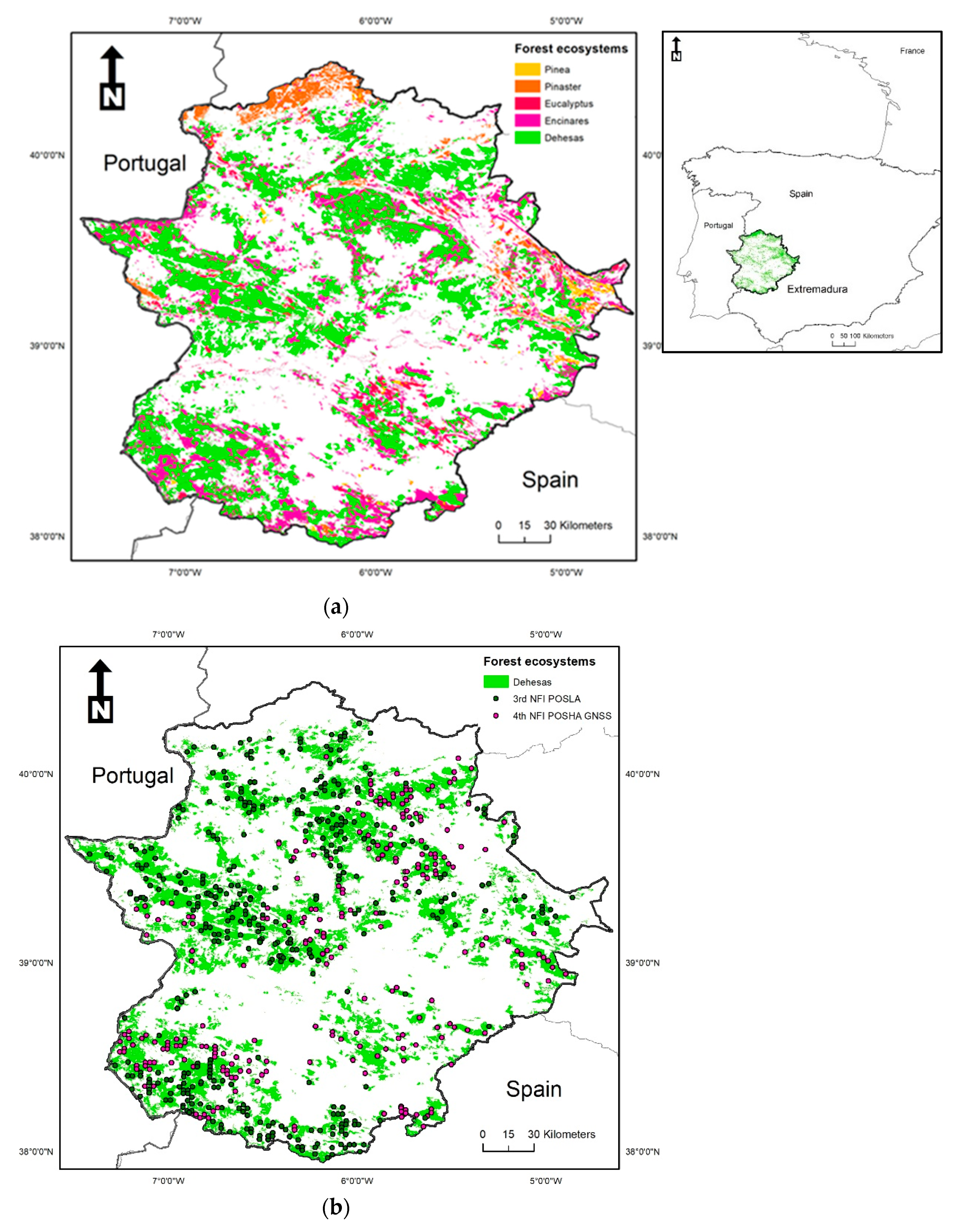
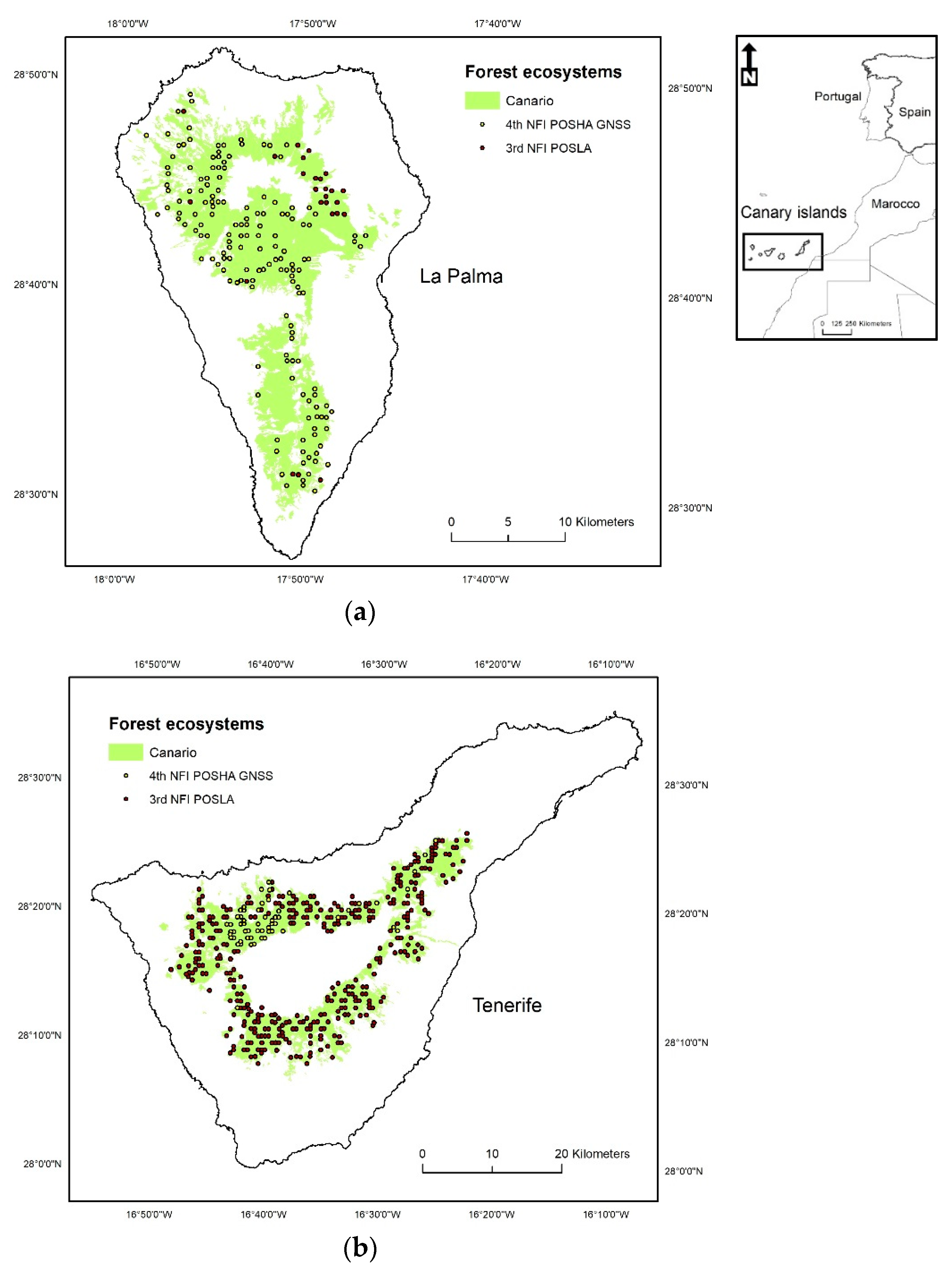
2.1. Study Area, Sampling Design and Ground Data

The study area is located in Spain, in the regions of Extremadura and the Canary Islands, covering 2.73 and 0.57 million hectares of forested landscapes. The region of Extremadura is located in continental Spain, in proximity to Portugal (Figure 1). The diversity of forest ecosystems is high, ranging from Atlantic areas to Mediterranean forests, including also agroforestry systems, which are the drivers of local economies based on farming. The Canary Islands comprise some of the most singular forest ecosystems in Europe due to their proximity to Africa and the presence of abrupt valleys, which act as reservoirs of endangered forest ecosystems in mild conditions, such as the Laurasia or “Laurisilva” (Figure 2). The forest map of Spain and the sampling design of the National Forest Inventory (NFI) were used in this research to cover a wide spectrum of forest structures. We selected seven forest ecosystems that have a minimum of 100 NFI sampling plots. The first five forest ecosystems listed are located in Extremadura, while Canario and Fayal-Brezal refer to the Canary Islands, and especially to the islands of Tenerife, La Palma and Gran Canaria, where most forest areas are located. The descriptions of the forest ecosystems and their notation used in the research are as follows:

• Dehesa: sparse old-growth cork oak forests (Quercus suber L.) of low tree density, “Dehesas”, traditionally managed to produce cork and provide grazing for domestic and wild livestock.
• Encinar: sparse oak forest (Quercus ilex subsp. ballota (Desf.) Samp.) managed in a coppice rotation system to produce firewood and grazing for domestic and wild livestock.
• Pinaster: even-aged forests of Pinus pinaster subsp. mesogeensis Aiton.
• Eucalyptus: commercial forests of Eucalyptus spp.; the dominant especies is Eucalyptus camaldulensis Dehnh., which is used to be managed for pulp.
• Pinea: even-aged forests of Pinus pinea L. managed for cone production and oriented to provide important ecosystem services over sandy soils, such as soil erosion control.
• Canario: dense even-aged forests of Pinus canariensis C. Sm. that provide important forest ecosystems services, such as erosion control in steep terrains. Fayal-Brezal: the wax myrtle-tree heath (‘Fayal-Brezal’) forest is a mixture of laurel tree (Familia Lauraceae) and Myrica faya Ait. trees and Erica arborea L. arboreal shrubs.

The sampling design in the NFI of Spain allows the variation of sampling size depending on tree diameter at breast height (1.3 m, dbh) as the statistitical inference based on circular plots with four concentric sub-plots, as follows: (i) Trees with dbh of at least 7.5 cm were measured using a plot radius of 5 m. (ii) Trees with dbh larger than 12.5 cm were measured in samples of 10-m radii. (iii) Trees with dbh larger than 22.5 cm were measured in the third plot radius (15 m). (iv) In the last concentric 25 m plot, all trees with dbh larger than 42.5 cm were measured. For more details about the NFI of Spain, see Alberdi et al. [34]. In the 3rd and 4th rounds of the NFI in Spain, ground measurements for both regions were collected, including tree diameters, species and the relative positions of all tress within a plot, were recorded and refered to the centre of the sample plot. The heights of all trees were recorded in the plots. The convesion of tree-level measuremetns into plot-level estimates resulted in the following characteristics for the sample plots (

Table 1. Summary of ground data collected in the 4th National Forest Inventory (NFI) for the seven forest ecosystems. Plot-level estimates are presented for stand basal area (G, m² ha⁻¹), tree density (N, trees ha⁻¹), growing stock volume (V, m³ ha⁻¹) and mean tree height (HT_mean, m).

Forest Ecosystem	Sample Plots	Statistic	HTmean (m)	G (m2 ha−1)	V (m3 ha−1)	N (trees ha−1)
Dehesa	499	Mean	7.7	6.5	15.3	85.0
		Max	14.1	27.8	62.6	1143.0
		Min	3.4	0.7	1.2	5.1
Encinar	275	Mean	5.9	4.9	15.8	272.0
		Max	11.7	31.3	108.6	2132.0
		Min	2.9	0.4	1.2	5.1
Pinaster	180	Mean	11.7	20.1	126.1	488.0
		Max	13.1	75.8	452.7	3214.9
		Min	4.6	0.4	1.6	5.1
Eucalyptus	163	Mean	11.6	7.2	42.2	390.7
		Max	24.9	47.8	396.5	1651.3
		Min	4.3	0.4	2.1	5.1
Pinea	113	Mean	9.2	13.9	63.7	360.4
		Max	17.7	64.4	426.8	2383.7
		Min	3.6	0.4	2.2	5.1
Canario	880	Mean	13.3	18.4	132.6	302.7
		Max	31.3	84.9	784.4	2574.7
		Min	2.8	0.4	1.6	5.1
Fayal-Brezal	210	Mean	8.1	23.8	105.6	1527.8
		Max	17.7	85.8	423.0	4806.8
		Min	3.4	0.4	1.5	5.1

). The estimation of volume was computed at tree-level using equations from the NFI protocol before upscaling the values to plot-level estimates. The final sampling set used as ground data comprised 2320 sample records from the 4th NFI (collected during 2016–2017 in both regions), including tree density (N, trees ha⁻¹), basal area (G, m² ha⁻¹), growing stock volume (V, m³ ha⁻¹) and mean tree height (HT_mean, m).

2.2. Positioning Equipment and Co-Registration Assessment

In this study, the center coordinates of the 2320 sample plots were available from the previous round of NFI measurements (3rd NFI). The location of NFI samples in Spain was conducted based on orthoimagery and cartographic maps over a 1 km square grid covering the whole country. The registration of new NFI sample plots during the 4th NFI was improved, compared to the field positioning methods used in the 3rd NFI. Hereby, the ongoing 4th round of the Spanish NFI is addressing the measurements of sample plots using modern GNSS equipment to improve plot positioning. The 4th NFI campaign in the Canary Islands and Extremadura used the TRIMBLE Juno 5B Handheld (Trimble Inc., USA), which can achieve real-time positioning accuracies between 2–4 m that can decrease to 1–3 m in the post-processing. As a showcase example, similar GNSS technology has been recently used in the NFI of Italy [35]. In the case of the NFI of Spain, Fernández-Landa et al. (2018) [3] also observed a mean error of 8.6 m, using the 4th NFI data from Spain, between the nominal coordinates available from previous rounds of the NFI of Spain and the new coordinates measured with commercial-grade GNSS equipment.

During field data collection in the 4th round of NFI measurements, a set of 877 NFI samples registered during the 3rd NFI were identified and inspected in the field to be re-measured using commercial-grade GNSS. The re-measurement samples represent 38% of the whole set of 2320 sample plots included in the study (

Table 2. Proportion of the sampling dataset measured both in the 3rd and 4th campaigns of the National Forest Inventory (NFI) using traditional plot positioning methods in the NFI (POS_LA) when using Global Navigation Satellite System (GNSS) equipment (POS_LA).

Positioning Accuracy	Forest Ecosystem
	Dehesa	Encinar	Pinaster	Eucalyptus	Pinea	Canario	Fayal Brezal
POSLA only	302	187	130	96	73	553	102
POSLA and POSHA	197	88	50	67	40	327	108
Re-measurement (%)	39.5	32.0	27.8	41.1	35.4	37.2	51.5
Total samples	499	275	180	163	113	880	210

). To control the bias from harvesting operations and natural disturbances in our research, and based on previous studies [36], only sample plots showing non-negative increments in forest attributes between the 3rd and 4th campaigns of the NFI were considered. The size of the training data to build the estimation models is within the range that other studies have identified as optimal to conduct ALS-based inferences [37]. In the next sections of the manuscript, we evaluate the use of two sets of measurements under the ABA approach. The ground data correspond to the recent 4th round of the NFI, in which measurements took place between 2016 and 2017. The coordinates used to conduct the ABA were used to split the data into two categories: The NFI samples for which coordinates were collected using a low-accuracy positioning in the traditional NFI (used in the 3rd NFI) will be denoted as POS_LA, while the recent positions measured in the 4th round (38% of the samples) with commercial-grade GNSS will be referred as POS_HA. The spatial layouts of the NFI-based sampling designs are presented for three forest ecosystems as showcases (Figure 1 and Figure 2).

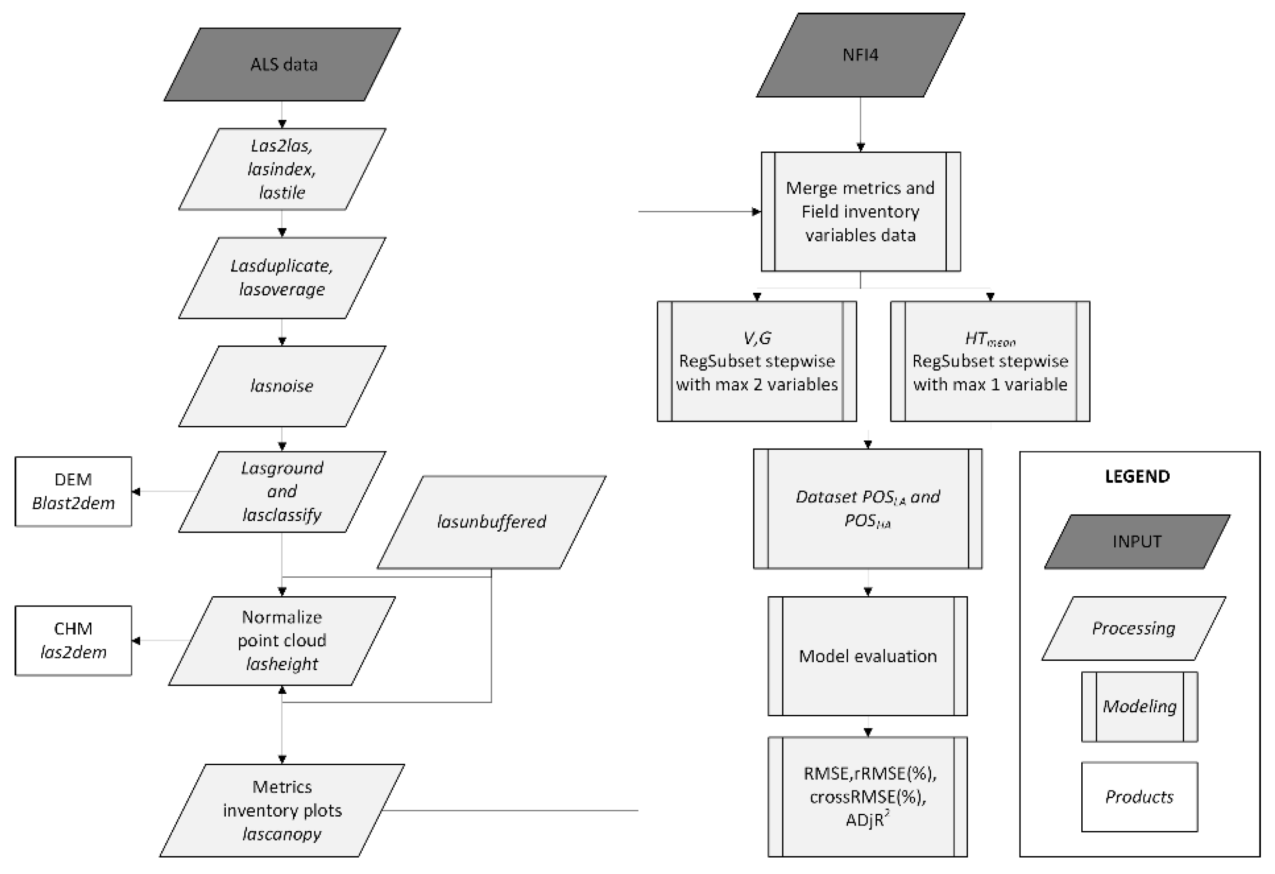
2.3. Airborne Laser Scanning

Two sets of ALS point clouds collected in different years were processed in this study: The ALS data for Extremadura were collected between July and September 2010, while the ALS campaign in the Canary Islands took place in 2015–2016. The time gap between NFI ground data collection and ALS surveys acquisition was 3 years for the Canary Islands and 7 for Extremadura, both within the feasible range to produce reliable estimates [38]. Both datasets correspond to the first (Extremadura) and second (the Canary Islands) round of nationwide ALS measurements, which are publicly available in Spain through the National Program of Aerial Orthophotography of Spain (PNOA). The nominal laser pulse density was 0.5 first returns m⁻² in Extremadura and 1 first returns m⁻² in the Canary Islands, respectively. The horizontal accuracy of scanning survey was 0.20 m in both datasets, while the vertical accuracy of ALS measurements was 0.20 m and 0.15 m in Extremadura and the Canary Islands, respectively. The scanning operations involved in the collection of the ALS data in the region of Extremadura used the LEICA ALS50 sensor operated at 1064 nm; the maximum pulse repetition rate was 83 kHz, the maximum scan frequency was 32.1 Hz, the maximum scanning angle was ± 50° and the average altitude during the scanning was 2866 m above the ground level. The specified scanning equipment recorded a maximum of four returns per pulse. The extension of the ALS data in both cases was very large, and the ALS processing was carried out using a manageable set of tiles (2 km² each).

The licensed software Lastools version 180620 [39] was used to process the ALS data. The ALS processing workflow within the Lastools environment comprised several steps (Figure 3). A total of 12058 and 2527 tiles were generated using lastile (parameters: tile_size = 2000 m, buffer = 50 m) in Extremadura and the Canary Islands, respectively. Secondly, tiles were filtered to remove noise using lasduplicate (parameters: unique_xyz) and lasnoise (parameters: step_z = 4, isolated = 5) and lasoverage to classify the overlap. Then, an ALS-derived point cloud was used to compute a digital terrain model (DTM) and a canopy height model (CHM). Firstly, ground points were classified using a progressive triangulated irregular network densification algorithm implemented in lasground_new (settings: step = 25 m, bulge= 2 m and offset = 0.05 m), and a 2 m DTM was created using the blast2dem. Lasclassify was used to discriminate between buildings and vegetation, and Lasheight were used to normalize the point cloud data. Then, raster layer metrics of vertical structures were extracted as follows, using lascanopy: The center plot coordinates from the 3rd NFI (POS_LA) and the new GNSS-based measurements from the 4th NFI data (POS_HA) were used to compute the ALS statistics that correspond to each sample plot. The last concentric buffer of 25 m radius in the NFI samples was used to clip the normalized ALS point clouds. The above-ground heights of ALS echoes were used to distinguish between tree canopies (echoes above 2 m) and the shrub layers (echoes below 2 meters) when computing ALS density and height statistics (lascanopy parameters: height_cutoff = 2, cover_cutoff = 2). The resulting set of 23 ALS statistics (

Table 3. Set of statistics derived from airborne laser scanning data used as candidate predictor variables to build the estimation models.

*Statistic	Symbol	Description
Moment statistics
Central tendency	Hmean	Mean elevation of ALS echoes.
Skewness	Hskew	Skewness of the distribution of ALS echoes.
Kurtosis	Hkurt	Kurtosis of the distribution of ALS echoes.
Order statistics	Hmax HMin	Maximum and minimum elevation of ALS echoes.
	CRR	Canopy Relief Ratio defined as (Hmean − HMin)/(Hmax − HMin).
Height percentiles	Hi for i = 1, 5, 10, 20, 25, 30, 40, 50, 60, 70, 75, 80, 90, 95, 99	Height percentiles of the ALS echoes distribution.
Density metric
Percent all > 2 m	FCall	Number of all points above 2 m divided by the number of all returns.
Cover metric
Percent first > 2 m	FCfirst	Number of first returns above 2 m divided by the number of all first returns as a percentage.

* Further explanation of the variables can be consulted in the LasTools manual [36].

) computed for each sample plot was used as candidate predictor variables in the model building stage.

2.4. Estimation of Forest Attributes

The estimation of forest attributes using statistics derived from 3D point clouds has been widely applied for ALS-based inventory [39]. The set of possible modeling techniques to be applied for the purpose is rich and of different complexity, ranging from simple linear regression methods to machine-learning algorithms [40,41,42,43]. As the level of influence of plot-positioning errors on data co-registration can differ between forest ecosystems, we sought for the ease of detection of worsening relationships between ground and ALS data rather than building complex models to promote model error minimization. We followed the maxima, “making simple models while possible without compromising their description of the phenomena” [44]. Multiple linear regression was preferred for simplicity and to compare previous studies using the same modeling technique to detect the impact of errors on data co-registration [11,12,17]. The modeling dataset for each of the seven forest ecosystems comprised models for stand basal area (G, m² ha⁻¹), growing stock volume (V, m³ ha⁻¹) and mean tree height (HT_mean, m). The already documented low predictive capability of stand density models was the reason to finally remove stand density from the fitting dataset [9,10].

The first step in the modeling phase was to select the optimal set of predictor variables to be used in the estimation of forest attributes. The leaps package [45], which is available for R statistical software [46], was tested to compute all possible combinations of predictors of certain arrays. In this study, we proposed the use of two predictors to estimate stand basal area and growing stock volume, while, for the case of mean tree height, we relied on one-parameter linear models. The described variable selection method was applied to both POS_HA and POS_LA in each forest ecosystem. The smallest root mean squared error (RMSE), the total explained variance (adjusted R²) and bias were used as the criteria for the selection of models [47,48]. The relative RMSE (RMSE%) values were calculated as the percentage of the average ground value of the given forest attributes. The implemented methodology to filter, process and to conduct ALS-based inventory is presented in Figure 3.

2.5. Inoptimality-Losses Approach and Co-Registration Assessment

The selection of predictor variables under the POS_LA and POS_HA was applied to estimate forest attributes for each studied forest ecosystem. The evaluation of plot positioning errors has previously determined the cost of biased selections of predictors [48]. The model transferability approach [25] can be further tested by evaluating the effect of the improved co-registration when sample plots are re-measured using commercial-grade GNSS positioning. In this study, the shift from low-accuracy positioning (POS_LA) versus high-accuracy positioning (POS_HA) is evaluated using the inoptimality losses approach concept under modern ALS-based forest inventory. The assessment aims at determining the reduction and increment in terms of RMSE% when co-registration thresholds between dependent and independent variables do not match. Hereby, the transferability model approach was evaluated as follows: we tested (i) the expected improvement of models built under low-accuracy positioning (POS_LA) when fitted with data corresponding to samples measured under high-accuracy positioning (POS_HA) and (ii) the expected worsening effect of transferring models built using POS_HA data when used with ALS statistics computed using POS_LA data. The model RMSE was firstly computed for each of the forest attributes estimated using the data from POS_HA and POS_LA. Then, the transferability of models was assessed in the following manner: the model built from the POS_LA was applied to predict the data from POS_HA, and vice versa, to compute the RMSE, called here as CrossRMSE. The RMSE and the CrossRMSE were computed as follows:

$${\mathrm{RMSE}}_{\mathrm{HA}}=\sqrt{\frac{{{\displaystyle \sum }}_{i=1}^n{\left(Y_{HA} - \widehat{Y_{M_{HA}}^{HA}} \right)}^2}{n_{HA}}},$$

(1)

$${\mathrm{RMSE}}_{\mathrm{LA}}=\sqrt{\frac{{{\displaystyle \sum }}_{i=1}^n{\left(Y_{LA} - \widehat{Y_{M_{LA}}^{LA}} \right)}^2}{n_{LA}}},$$

(2)

$${\mathrm{CrossRMSE}}_{\mathrm{LA}}=\sqrt{\frac{{{\displaystyle \sum }}_{i=1}^n{\left(Y_{LA} - \widehat{Y_{M_{HA}}^{LA}} \right)}^2}{n_{LA}}},$$

(3)

$${\mathrm{CrossRMSE}}_{\mathrm{HA}}=\sqrt{\frac{{{\displaystyle \sum }}_{i=1}^n{\left(Y_{HA} - \widehat{Y_{M_{LA}}^{HA}} \right)}^2}{n_{HA}}},$$

(4)

where RMSE_HA and RMSE_LA are the RMSE values for models (M_HA and M_LA) when using the ground data and ALS statistics of POS_HA and POS_LA datasets; n_HA and n_LA are the number of sample plots of POS_HA and POS_LA. Model predictions are denoted by ($\hat{\mathrm{Y}}$). For instance, the term $Y_{M_{HA}}^{HA}$ accounts for the prediction when using the ALS statistics and ground data of POS_HA. Equations (3) and (4) account for the CrossRMSE. In Equation (3), for instance, the model built with POS_HA data was used to predict forest attributes using ALS statistics of POS_LA data, and the RMSE% was computed using ground data of POS_LA. The RMSE and CrossRMSE values were scaled to relative values to express the percentage over the average value of the three forest attributes included in POS_HA and POS_LA datasets.

3. Results

3.1. Selection of Predictor Variables and Model Building

The horizontal distance between ground sample positions in POS_HA and POS_LA was computed in both study areas, where the field crew identified sample plots on the ground before the plot center was measured again by using the commercial-grade GNSS (

Table 4. Distance between sampling positions in the 3rd and 4th National Forest Inventory (NFI). The mean value and the standard deviation of the computed distances are presented for the selected forest ecosystems.

Forest Ecosystem	Mean Distance (m)	Distance Range (m)	Standard Deviation (m)
Dehesa	21.1	0.5–90.6	12.9
Encinar	21.4	4.0–63.5	13.4
Pinaster	29.5	0.8–85.5	19.2
Pinea	22.9	0.7–57.8	16.9
Eucalyptus	22.5	2.3–90.6	14.4
Canario	29.5	1.6–249.7	35.2
Fayal-Brezal	30.1	2.3–119.5	28.0

). The results pointed out the discrepancy between both positioning sources. The mean difference in the positioning records was 22.6 m, ranging from 21 m for the sparse Encinar and Dehesa forests to 30.2 m in the dense Fayal-Brezal forests. The observed deviation of POS_LA horizontal coordinates from POS_HA coordinates (assumed ground truth) was 90 m in the Extremadura dataset and reaching almost 250 m for the Canario forests. The standard deviation of the distances showed more variability in the Canary Islands, where NFI samples located in the Canario forests had higher values than those computed for Extremadura.

3.2. Selection of Predictor Variables and Model Building

The observed variation on the distribution of ALS echoes (Figure A1 and Figure A2 and Appendix A) was further assessed towards the composition of the models. The selection of variables pointed out the good performance of density and height-based statistics to estimate both growing stock volume and stand basal area. The selected optimal predictor variables for the models built from the POS_LA datasets were similar to when using the POS_HA datasets. At least one density statistic was selected in all models for growing stock volume and stand basal area in both positioning conditions. The selection of the best predictor to estimate mean tree height remained similar for POS_LA and POS_HA datasets in all tested forest ecosystems, except for the Dehesa forest, for which the selection shifted from H₄₀ to H₉₉ (

Table 5. Selection of predictor variables using low-accuracy positioning methods (POS_lA) and commercial-grade GNSS positioning (POS_HA).

Forest Attribute	Forest Ecosystem
	Dehesa	Encinar	Pinaster	Eucalyptus	Pinea	Canario	Fayal Brezal
POSLA
Mean tree height (HTmean, m)	Hmean	H40	H70	H90	Hmean	Hmean	H99
Basal area (G, m2 ha−1)	Hmax	Hkur	H10	Hstd	FCfirst	H50	H01
	FCfirst	FCfirst	FCfirst	FCall	FCall	FCfirst	H25
Volume (V, m3 ha−1)	Hstd	H10	H01	Hstd	FCfirst	H25	H30
	FCfirst	FCfirst	FCfirst	FCall	FCall	FCfirst	FCfirst
POSHA
Mean tree height (HTmean, m)	Hmean	H99	H80	H80	Hstd	H50	H40
Basal area (G, m2 ha−1)	H99	H95	H25	Hstd	FCfirst	FCfirst	FCfirst
	FCall	FCall	FCall	FCall	H20	H40	H20
Volume (V, m3 ha−1)	H01	H40	H10	H50	H10	CRR	FCall
	FCfirst	FCfirst	FCall	FCall	FCfirst	FCfirst	FCfirst

Note: Model coefficients are presented in Appendix B (Table A1).

). The benchmark between the set of models for POS_LA to POS_HA was further assessed by comparing the accuracy of the linear models using RMSE% and the total explained variance. Increasing the co-registration mismatch by using low-accuracy positioning reduced the efficiency of the models (

Table 6. Goodness of the model fitting expressed by the R-squared value in bold and the computed RMSE% between parentheses. The results are presented for seven forest ecosystems considering low- accuracy positioning methods (POS_LA) and commercial-grade GNSS positioning (POS_HA).

Forest Attribute	Forest Ecosystem
	Dehesa	Encinar	Pinaster	Eucalyptus	Pinea	Canario	Fayal Brezal
POSLA
Mean tree height (HTmean, m)	0.70	0.45	0.65	0.62	0.59	0.49	0.46
	(11.2)	(16.9)	(15.2)	(16.8)	(16.8)	(25.1)	(25.5)
Basal area (G, m2 ha−1)	0.45	0.57	0.66	0.60	0.69	0.65	0.45
	(42.3)	(55.4)	(41.8)	(54.0)	(44.3)	(47.6)	(62.4)
Volume (V, m3 ha−1)	0.50	0.46	0.67	0.57	0.61	0.67	0.61
	(46.6)	(73.0)	(46.0)	(72.7)	(58.5)	(55.8)	(62.2)
POSHA
Mean tree height (HTmean, m)	0.70	0.65	0.69	0.81	0.81	0.67	0.46
	(11.2)	(17.0)	(12.0)	(12.1)	(12.1)	(22.9)	(22.6)
Basal area (G, m2 ha−1)	0.35	0.40	0.79	0.71	0.83	0.65	0.68
	(40.1)	(50.3)	(29.3)	(48.5)	(24.6)	(37.7)	(43.0)
Volume (V, m3 ha−1)	0.31	0.50	0.78	0.78	0.83	0.77	0.74
	(45.0)	(62.6)	(33.2)	(56.1)	(30.7)	(35.9)	(46.7)

). The scale of the effect significantly differed when comparing forest ecosystems. For instance, the increment in the RMSE% for stand basal area ranged from 2.1% for the Dehesa forest ecosystem to 19.9% in the Pinea forests. For the growing stock volume, the RMSE% ranged from 1.6% to 27.8% in both forest ecosystems, respectively. The trends for both forest attributes were similar, except for the case of the Eucalyptus, for which the worsening effect reached 5.8% for stand basal area but increased up to 16.6% for the volume. The cost of low-accuracy positioning when modeling mean tree height was less than 5% in all cases; the difference between POS_LA to POS_HA was less than 1% for the Dehesa and the Encinar, progressively increasing to 2.3% (Canario), 2.9% (Fayal-Brezal), 3.2% (Pinaster) and 4.7% (Eucalyptus and Pinea). The difference between the computed RMSE% values from the co-registration factor is presented in (Figure 4).

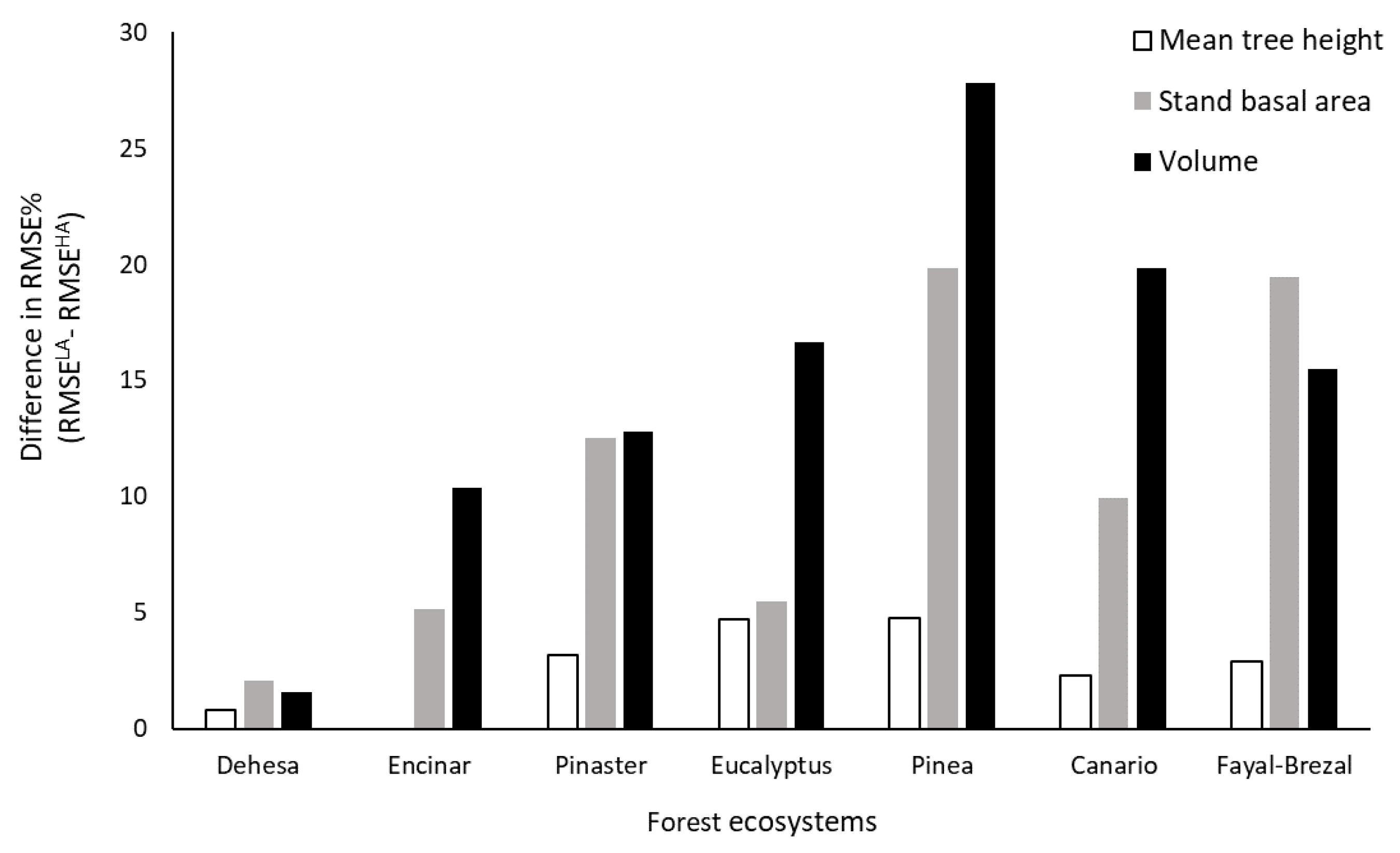
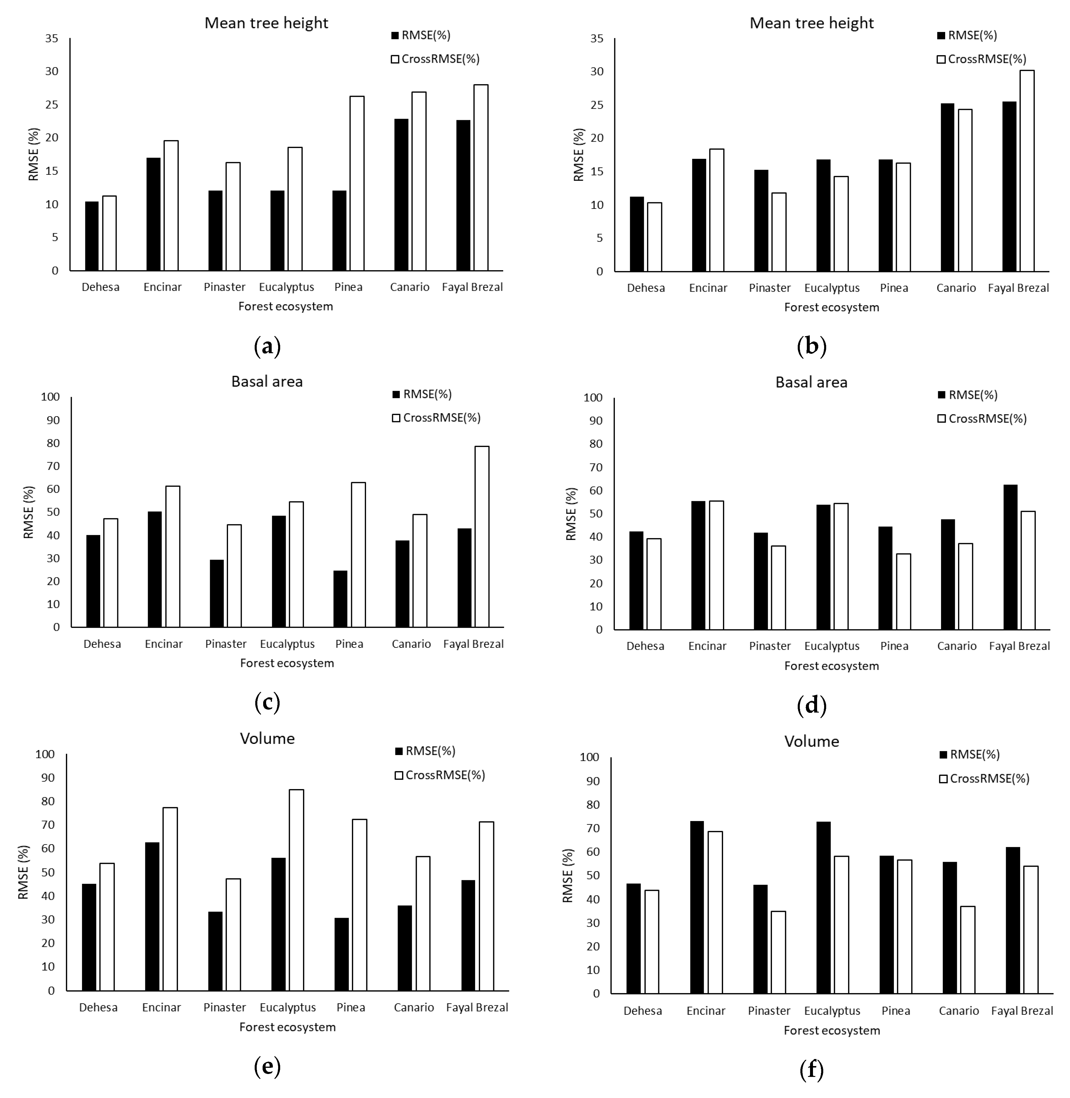
3.3. Assessing the Transferability Approach

3.3.1. Mean Tree Height Models

The expected improvement of using POS_LA models for mean tree height with POS_HA data was not observed for both the Encinar and Fayal-Brezal ecosystems; no RMSE reduction was observed from enhancing data co-registration. The improvement for the other five cases ranged between 0.9% (Dehesa) to 3.4% (Pinaster) points in the RMSE%. The scale of the benefit was lower for mean tree height compared to the basal area growing stock volume, as expected (Figure 5a,b). The RMSE% increased when using POS_HA models with POS_LA data, reaching the maximum for the Pinea forest ecosystem (14.2%), followed by the Eucalyptus (6.5%).

3.3.2. Stand Basal Area Models

The use of basal area models built for POS_LA and ground data from POS_HA datasets resulted in a reduction of the RMSE% by 10%–11% for Pinea, Canario and Fayal-Brezal (Figure 5c,d). The computed decrement was substantially lower for Dehesa (3.2%), Encinar (0.1%) and Pinaster (5.7%). The increment in the computed model error (CrossRMSE%–RMSE%) when using POS_HA models with POS_LA datasets was used to classify forest ecosystems as: (i) low impact computed for Eucalyptus (5.9%) and Dehesa (6.9%); (ii) medium impact for Encinar (11.0%), Pinaster (15.2%) and Canario (11.2%) and (iii) high impact for the Canario and Pinea forests, which had an increment of 35.5% and 38.2%, respectively.

3.3.3. Growing Stock Volume Models

Similarly, as with stand basal area, the largest improvement in the estimation of volume was computed for the Canario forest ecosystems, for which POS_LA models improved 18.9% on RMSE% when fitted with POS_HA data (Figure 5e,f). The improvement was also higher for Eucalyptus and Pinaster, while for the rest of the forest ecosystems, the improvement was below 3%. In the opposite scenario, transferring models for the growing stock volume from high-accuracy to low-accuracy co-registration resulted in greater impacts compared to the basal area. For instance, the increments in the computed RMSE% increased between 8.8% and 41.7% points in the RMSE% for Dehesa and Pinea, respectively.

4. Discussion

The combined use of NFI sampling designs and nationwide ALS data ensures a robust estimation and prediction of forest attributes due to the scale of sampling campaigns [23], as long as certain operational and technical requirements are met [9]. The use of NFI data with ALS-based applications has always been constrained due to an important and frequent source of uncertainty when interpreting ALS data and related to ground data collection: co-registration. The accuracy in the collection of plot locations using commercial-grade GNSS is then a cornerstone factor to conduct a good statistical inference [10]. Furthermore, we evaluated in this paper the implications of improving the co-registration between ground and ALS data by means of modern plot positioning methods on two regional-scale inventories based on the sampling design from the NFI of Spain. We compared modeling results from two sets of measurements. Ground NFI data corresponded to the 4th NFI in all cases, but the coordinates of the NFI samples were registered under two different conditions in terms of data co-registration goodness: (i) using traditional positioning methods in the 3rd NFI (POS_LA) and new coordinates registered with GNSS equipment during the 4th NFI ground campaign (POS_HA). The outcomes of the research pointed out the benefit of using better georeferenced data, although the level of improvement needs to be carefully assessed considering the complexity of the forest structure, as previously suggested in small-scale experiments [11,12].

The results of the study showed the slight benefit of improved data co-registration in sparse forest ecosystems, where errors for stand basal area models are already considerably high. The benefit of re-measuring sample plots with high-accurate GNSS for the Dehesa ecosystem were minor compared to the level of improvement in other, denser forest ecosystems. The density and structural complexity of the Quercus ilex forests (Encinar) is greater than in the Dehesa, and the results showed an improvement that reaches 10% for volume and 5% for stand basal area in terms of RMSE%. The case of stone pine forests (Pinea) needs further analysis, since the models should have behaved similarly as in Dehesa and Encinar due to the sparse tree spacing in stone pine forests [17]. However, the stone pine forests in Extremadura are different compared to, for instance, the Northern Plateau [49], in which the spatial distribution of trees is certainly sparse [11,12]. The stone pine forests in Extremadura are more densified. Therefore, the structural complexity of Pinea sample plots is high, and this can explain the high effect of good data co-registration when fitting models for volume and stand basal area: the scale of the improvement was 20% in both cases in terms of RMSE%, increments from 0.59 to 0.83 and 0.69 to 0.83 in terms of R² for volume and stand basal area, respectively. As the computation of growing stock volumes requires the application of models to predict individual tree volumes (with their associated model error), we found it more logical to base the assessment of data co-registration using stand basal area and tree height variables. The improvement in basal area models for the densely vegetated Fayal-Brezal samples was also considerable when using POS_HA data. This impact was greater than for Pinaster and Eucalyptus forests, which models already have good accuracy (R² above 0.7 in POS_HA and above 0.6 in POS_LA). In cases of sparse forest ecosystems, where data co-registration has a minor effect [17], the forest managers might need to implement additional improvements. The usability of stand basal models under the traditional ABA method is being discussed by forest managers and technicians in the Extremadura Forest Service due to the potential overestimation of forest attributes in the Dehesa forests when predicting forest attributes and comparing them with the estimations from the ITC approach. A good approach to improve estimation models is to rely on individual tree detection methods combining active and passive sensing [50,51] and enhanced area-based approaches, combining ABA and individual tree detection [17]. Those methods can improve the robustness of ALS-based inference, but, at the same time, the positioning factor can become more restrictive: the shift from area-based to tree-level forest inventory requires the positioning of ground tree measurements to validate the results from tree detection algorithms. Therefore, the investment in improving data co-registration is critical, no matter the forest inventory approach tested under the array of possible modern ALS-based methods.

The selection of predictor variables also revealed important patterns. The density metrics were used for a high proportion of the models in the set for basal area and volume. For example, the proportion of first ALS vegetation echoes above certain height thresholds is a good indicator of forest stocking. However, the variability of density statistics towards the occurrence of plot positioning errors is greater compared to height-based percentiles. The scale of positioning errors influences more the number and the distribution of ALS echoes in the presence of gaps compared to top height percentiles (i.e., the maximum elevation of tree canopies), which are prone to be detected by lasers despite the occurrence of low-scale errors in plot positioning operations [12]. Therefore, and in light of the model performances for basal area and volume, the use of density statistics can lead to a worsening performance of the models under bad data co-registration goodness due to their variability in the presence of gaps and discontinuities. Forthcoming studies need to address the cost of including more height-based predictors in the volume and stand basal area models, which makes them more stable towards the impact of plot positioning errors when computing ALS statistics but, at the same time, less accurate compared to density-metrics-based models. For the case of mean tree height models, the scale of the improvement from POS_LA to POS_HA is lower, as expected, and the results confirmed that improving co-registration in certain forest ecosystems (e.g., Dehesa and Encinar) can have barely no impact on tree height models. The reason for the different behaviors between stand basal area models and mean tree height models are again related to model predictors: (i) even in the presence of high co-registration errors, the ALS data can detect the maximum elevation of the echoes if the height profile of tree vegetation in the surroundings of the plot remains homogeneous and( ii) the presence of gaps reduce the number of ALS echoes corresponding to forest vegetation, and this impacts the computation of density statistics, which is based on the ratio between the number of ALS echoes that hits forest vegetation in the enumerator and the total number of ALS echoes in the denominator [38].

The tested modeling approach was simple and oriented to detect shifts in the predictive capability of the models in the presence of the positioning errors that altered data co-registration between ground and ALS data. Using more sophisticated and contemporary inference methods could have reduced model errors [41], but the idea of the paper was to keep the models as simple as possible, which is perfectly valid in ALS-based forest inventory. Among the set of possible improvements in the models, the statistical inference can acknowledge structural relationships between dependent variables to conform a system of nested but simple models rather than increasing the complexity of the models individually [52,53]. The efficiency of ABA models for the case of POS_LA was poor, as expected, due to the uncertainty in field data protocols in the successive rounds of the NFI in Spain. The horizontal mean error between POS_HA positioning and their previous coordinates in the 3rd NFI was 26.2 m, which explains the reported values in other studies. The dataset used in the research is very valuable; the POS_HA represents the first opportunity to conduct forest inventory using ALS and sample plots from the NFI of Spain registered under good data co-registration. Our results showed that models built with poorly co-registered data can perform better when transferred to a new forest area following the timely model transferability approach.

The principle of the transferability approach is to use ALS models to predict the forest attributes for a different dataset that was not used to build the model. Such approaches are normally required by forest managers, who frequently avoid collecting more data for the modeling, especially when public nationwide datasets are used. Furthermore, the cost of analysis can be reduced, since independent variables do not require investments for their collection, as occurred with the PNOA in Spain. The reasoning of the transferability approach is not restricted to assessing spatial transferability between forest areas but also to measure the benefit (or penalty) of using ALS statistics that do not completely correspond to the ground observations as a result of uncertainty when registering plot coordinates [12]. On one side, models built under good co-registration quality were more sensitive to their calibration when poorly co-registered data was used, as expected. On the other, there is a benefit when good co-registered data is used to transfer “bad” models to a new area, which is the main outcome of our assessment. In simple words, improved GNSS positioning increases the accuracy of forest attribute predictions through ALS data. The computed improvement of the models under the implemented inoptimality losses approach was high, reaching a RMSE% of almost 30% in some cases for volume and stand basal area.

The revision of the sample plots requires verifying that no human intervention in the sample plots, and also in the surroundings, has taken place. In this study, the sampling dataset was reduced from 4031 to 2320 due to the occurrence of negative variations between the 3rd and the 4th measuring campaign of the NFI. The occurrences of harvesting operations and natural disturbances must be addressed when accounting for spatial and temporal patterns in forest inventory [36]. We account for the loss of 40% of sampling records due to natural and human interventions, but the impact of disturbances might be greater, as the buffering zone around the sample plots can be affected. To control the homogeneity around NFI sample plots is a critical step to improve the usability of remote sensing in large-scale mapping, especially in the context of co-registration errors that can substantially impact the robustness of the statistical inferences, as we documented. The time gap between ground measurements and the collection of the ALS data is an important issue, especially in fast-growing species. In our research, the time gap was 1–2 years for the Canary Islands and 6–7 years for the Extremadura, which can be in the feasible threshold (years of the gap) based on previous studies [38]. The maximum lifespan of a certain ALS dataset can also depend on forest structure. For instance, ALS data collected for slow-growing species such as in Encinar or Dehesa can still be valid for a longer lifespan than for the case of the Eucalyptus of pine forests. Further research could evaluate the maximum ALS lifespans for a broader range of forest ecosystems in Extremadura, where the second round of scanning under the PNOA project is about to conclude.

The optimal integration of remote sensing data, and ALS in particular, into large-scale mapping using NFI data needs to account for improved data co-registration methods and also effective methods to preserve sampling areas. In this regard, it is important to recognize human-related disturbances and avoid the impact of edge effects [17], which is a real challenge, especially in fragmented forest landscapes composed of small-scale privately owned areas [23]. The addressing of growth dynamics based on multi-temporal NFI observations and using remote sensing data is the next challenge once the co-registration uncertainty is solved or, at least, mitigated [54,55,56].

The cost of the re-measurement operations of the whole set of NFI plots using commercial-grade GNSS equipment might exceed the resources of the NFI program. Operationally, and in budgetary terms, the task of re-visiting the whole set of NFI plots can overwhelming at once. The investment can gradually pay off if NFI forest managers can determine the minimum number of sample plots to be re-measured using improved positioning protocols. The search for the center points in NFI sampling designs can be extremely time-consuming, and, therefore, the effort should be progressive and continuous in the next rounds of NFI campaigns. Still, some questions remain, open and further evidence is needed to support our discussed model improvement that arose from the re-measurement of 877 samples from a total of 2320. Further studies are needed to define the optimal size of the NFI samplings in cases of ALS-based estimations on regional and national scales [21]. Based on the presented methodology and the very valuable dataset comprising hundreds of corrected NFI sample positions, the intensity of the NFI sampling design under ALS-based forest inventory can be further discussed, and this will be the core of a forthcoming research.

5. Conclusions

The research demonstrated the improvement in forest inventory when resources are invested to improve the co-registration between ground NFI data and ALS point clouds. The scale of the enhancement varied between forest ecosystems, depending on the structural complexity and the forest attributes analyzed. The usability of current NFI data under modern forest inventory approaches can be restricted when combining multiple remote sensing data sources. This research showed that investing in reducing data uncertainty when registering NFI sample plots improves the predictive capacity of ALS-based forest inventory while improving the usability of existing models when fitted to new areas lacking in ground attributes. The research evaluated the model transferability approach under a new dimension, shifting from model transferability between areas/regions to an implementation based on data sources collected under different data co-registration goodness.

References

1. Corona, P.; Chirici, G.; McRoberts, R.E.; Winter, S.; Barbati, A. Contribution of large-scale forest inventories to biodiversity assessment and monitoring. For. Ecol. Manag. 2011, 262, 2061–2069. [Google Scholar] [CrossRef] [Green Version]
2. Alberdi, I.; Condés, S.; Mcroberts, R.E.; Winter, S. Mean species cover: A harmonized indicator of shrub cover for forest inventories. Eur. J. For. Res. 2018, 137, 265–278. [Google Scholar] [CrossRef] [Green Version]
3. Fernández-Landa, A.; Fernández-Moya, J.; Tomé, J.L.; Algeet-Abarquero, N.; Guillén-Climent, M.L.; Vallejo, R.; Sandoval, V.; Marchamalo, M. High resolution forest inventory of pure and mixed stands at regional level combining national forest inventory field plots, Landsat, and low density lidar. Int. J. Remote Sens. 2018, 39, 14. [Google Scholar] [CrossRef]
4. Shang, C.; Coops, N.C.; Wulder, M.A.; White, J.C.; Hermosilla, T. Update and spatial extension of strategic forest inventories using time series remote sensing and modeling. Int. J. Appl. Earth Obs. 2020, 84, 101956. [Google Scholar] [CrossRef]
5. McRoberts, R.E.; Andersen, H.E.; Næsset, E. Using airborne laser scanning data to support forest sample surveys. In Forestry Applications of Airborne Laser Scanning; Maltamo, M., Næsset, E., Vauhkonen, J., Eds.; Managing Forest Ecosystems Book Series Volume 27; Springer: Dordrecht, The Netherlands, 2014. [Google Scholar]
6. Gschwantner, T.; Lanz, A.; Vidal, C.; Bosela, M.; Di Cosmo, L.; Fridman, J.; Gasparini, P.; Kuliešis, A.; Tomter, S.; Schadauer, K. Comparison of methods used in European national forest inventories for the estimation of volume increment: Towards harmonisation. Ann. For. Sci. 2016, 73, 807–821. [Google Scholar] [CrossRef] [Green Version]
7. Tomppo, E.; Haakana, M.; Katila, M.; Peräsaari, J. Multi-Source National Forest Inventory: Methods and Applications; Springer: New York, NY, USA, 2008; Volume 18. [Google Scholar]
8. White, J.C.; Coops, N.C.; Wulder, M.A.; Vastaranta, M.; Hilker, T.; Tompalski, P. Remote sensing technologies for enhancing forest inventories: A review. Can. J. Remote Sens. 2016, 42, 619–641. [Google Scholar] [CrossRef] [Green Version]
9. Wulder, M.A.; White, J.C.; Nelson, R.F.; Næsset, E.; Ørka, H.O.; Coops, N.C.; Hilker, T.; Bater, C.W.; Gobakken, T. Lidar sampling for large-area forest characterization: A review. Remote Sens. Environ. 2012, 121, 196–209. [Google Scholar] [CrossRef] [Green Version]
10. Vauhkonen, J.; Maltamo, M.; McRoberts, R.E.; Næsset, E. Introduction to forestry applications of airborne laser scanning. In Forestry Applications of Airborne Laser Scanning: Concepts and Case Studies; Maltamo, M., Næsset, E., Vauhkonen, J., Eds.; Managing Forest Ecosystems Book Series Volume 27; Springer: Amsterdam, The Netherlands, 2014. [Google Scholar]
11. Gobakken, T.; Næsset, E. Assessing effects of positioning errors and sample plot size on biophysical stand properties derived from airborne laser scanner data. Can. J. For. Res. 2009, 39, 1036–1052. [Google Scholar] [CrossRef]
12. Pascual, A.; Pukkala, T.; de-Miguel, S. Effects of plot positioning errors on the optimality of harvest prescriptions when spatial forest planning relies on ALS data. Forests 2018, 9, 371. [Google Scholar] [CrossRef] [Green Version]
13. Johnson, C.E.; Barton, C.C. Where in the world are my field plots? Using GPS effectively in environmental field studies. Front. Ecol. Environ. 2004, 2, 475–482. [Google Scholar] [CrossRef]
14. Pascual, A.; Bravo, F.; Ordoñez, C. Assessing the robustness of variable selection methods when accounting for co-registration errors in the estimation of forest biophysical and ecological attributes. Ecol. Model. 2019, 403, 11–19. [Google Scholar] [CrossRef]
15. Frazer, G.W.; Magnussen, S.; Wulder, M.A.; Niemann, K.O. Simulated impact of sample plot size and co-registration error on the accuracy and uncertainty of LiDAR-derived estimates of forest stand biomass. Remote Sens. Environ. 2011, 115, 636–649. [Google Scholar] [CrossRef]
16. Næsset, E.; Jonmeister, T. Assessing point accuracy of DGPS under forest canopy before data acquisition, in the field, and after postprocessing. Scan. J. For. Res. 2002, 17, 351–358. [Google Scholar] [CrossRef]
17. Pascual, A. Using tree detection based on airborne laser scanning to improve forest inventory considering edge effects and the co-registration factor. Remote Sens. 2019, 11, 2675. [Google Scholar] [CrossRef] [Green Version]
18. Mauro, F.; Valbuena, R.; Manzanera, J.A.; García-Abril, A. Influence of global navigation satellite system errors in positioning inventory plots for tree-height distribution studies. Can. J. For. Res. 2011, 41, 11–23. [Google Scholar] [CrossRef]
19. Gopalakrishnan, R.; Thomas, V.A.; Coulston, J.W.; Wynne, R.H. Prediction of canopy heights over a large region using heterogeneous lidar datasets: Efficacy and challenges. Remote Sens. 2015, 7, 11036–11060. [Google Scholar] [CrossRef] [Green Version]
20. Guerra-Hernández, J.; Bastos Görgens, E.; García-Gutiérrez, J.; Estraviz Rodriguez, L.C.; Tomé, M.; González-Ferreiro, E. Comparison of ALS based models for estimating aboveground biomass in three types of Mediterranean forest. Eur. J. Remote Sens. 2016, 49, 185–204. [Google Scholar] [CrossRef]
21. Junttila, V.; Finley, A.O.; Bradford, J.B.; Kauranne, T. Strategies for minimizing sample size for use in airborne LiDAR-based forest inventory. For. Ecol. Manag. 2011, 292, 75–85. [Google Scholar] [CrossRef]
22. Nord-Larsen, T.; Schumacher, J. Estimation of forest resources from a country wide laser scanning survey and national forest inventory data. Remote Sens. Environ. 2012, 119, 148–157. [Google Scholar] [CrossRef]
23. Novo-Fernández, A.; Barrio-Anta, M.; Recondo, C.; Cámara-Obregón, A.; López-Sánchez, C.A. Integration of national forest inventory and nationwide airborne laser scanning data to improve forest yield predictions in north-western Spain. Remote Sens. 2019, 11, 1693. [Google Scholar] [CrossRef] [Green Version]
24. Bontemps, J.D.; Bouriaud, O. Predictive approaches to forest site productivity: Recent trends, challenges and future perspectives. Forestry 2013, 87, 109–128. [Google Scholar] [CrossRef]
25. Korhonen, L.; Repola, J.; Karjalainen, T.; Packalen, P.; Maltamo, M. Transferability and calibration of airborne laser scanning based mixed-effects models to estimate the attributes of sawlog-sized Scots pines. Silva Fenn. 2019, 53, 1–18. [Google Scholar] [CrossRef] [Green Version]
26. Tompalski, P.; White, J.C.; Coops, N.C.; Wulder, M.A. Demonstrating the transferability of forest inventory attribute models derived using airborne laser scanning data. Remote Sens. Environ. 2019, 227, 110–124. [Google Scholar] [CrossRef]
27. Domingo, D.; Alonso, R.; Lamelas, M.T.; Montealegre, A.L.; Rodríguez, F.; de la Riva, J. Temporal transferability of pine forest attributes modeling using low-density airborne laser scanning data. Remote Sens. 2019, 11, 261. [Google Scholar] [CrossRef] [Green Version]
28. Fekety, P.A.; Falkowski, M.J.; Hudak, A.T.; Jain, T.B.; Evans, J.S. Transferability of lidar-derived basal area and stem density models within a northern Idaho ecoregion. Can. J. Remote Res. 2018, 44, 131–143. [Google Scholar] [CrossRef]
29. Kangas, A.; Gobakken, T.; Puliti, S.; Hauglin, M.; Naesset, E. Value of airborne laser scanning and digital aerial photogrammetry data in forest decision making. Silva Fenn. 2018, 52, 9923. [Google Scholar] [CrossRef] [Green Version]
30. Lindgren, N.; Christensen, P.; Nilsson, B.; Åkerholm, M.; Allard, A.; Reese, H.; Olsson, H. Using optical satellite data and airborne lidar data for a nationwide sampling survey. Remote Sens. 2015, 7, 4253–4267. [Google Scholar] [CrossRef] [Green Version]
31. Sankey, T.; Donager, J.; McVay, J.; Sankey, J.B. UAV lidar and hyperspectral fusion for forest monitoring in the southwestern USA. Remote Sens. Environ. 2017, 195, 30–43. [Google Scholar] [CrossRef]
32. Iglhaut, J.; Cabo, C.; Puliti, S. Structure from motion photogrammetry in forestry: A review. Curr. For. Rep. 2019, 5, 155–168. [Google Scholar] [CrossRef] [Green Version]
33. Bravo, F.; Gabriel, J.; del Rio, M.; Barrio, M.; Bonet Lledos, J.A.; Bravo Olviedo, A.; Calama, R.; Castedo Dorado, F.; Crecente Campo, F.; Condes, S.; et al. Growth and yield models in Spain: Historical overview, contemporary examples and perspectives. For. Syst. 2012, 20, 315–328. [Google Scholar] [CrossRef] [Green Version]
34. Alberdi, I.; Cañellas, I.; Vallejo, R. The Spanish national forest inventory: History, development, challenges and perspectives. Pesquisa Florestral Brasileira 2017, 37, 361. [Google Scholar] [CrossRef]
35. Chirici, G.; Giannetti, F.; McRoberts, R.E.; Travaglini, D.; Pecchi, M.; Maselli, F.; Chiesi, M.; Corona, P. Wall-to-wall spatial prediction of growing stock volume based on Italian national forest inventory plots and remotely sensed data. Int. J. Appl. Earth Obs. 2020, 84, 101959. [Google Scholar] [CrossRef]
36. Bolton, D.K.; Coops, N.C.; Wulder, M.A. Measuring forest structure along productivity gradients in the Canadian boreal with small-footprint Lidar. Environ. Monit. Assess. 2013, 185, 6617. [Google Scholar] [CrossRef]
37. Shin, J.; Temesgen, H.; Strunk, J.L.; Hilker, T. Comparing modeling methods for predicting forest attributes using LiDAR metrics and ground measurements. Can. J. Remote Sens. 2016, 42, 739–765. [Google Scholar] [CrossRef]
38. McRoberts, R.E.; Chen, Q.; Gormanson, D.D.; Walters, B.F. The shelf-life of airborne laser scanning data for enhancing forest inventory inferences. Remote Sens. Environ. 2018, 206, 254–259. [Google Scholar] [CrossRef]
39. Isenburg, M. LAStools-Efficient LiDAR Processing Software, version 14101; rapidlasso GmbH: Gilching, Germany, 2018; Available online: http://rapidlasso.com/LAStools (accessed on 24 April 2018).
40. Maltamo, M.; Næsset, E.; Vauhkonen, J. (Eds.) Forestry Applications of Airborne Laser Scanning: Concepts and Case Studies; Managing Forest Ecosystems Book Series Volume 27; Springer: Dordrecht, The Netherlands, 2014. [Google Scholar]
41. Gleason, C.J.; Im, J. Forest biomass estimation from airborne LiDAR data using machine learning approaches. Remote Sens. Environ. 2012, 125, 80–91. [Google Scholar] [CrossRef]
42. Fassnacht, F.E.; Hartig, F.; Latifi, H.; Berger, C.; Hernández, J.; Corvalán, V.; Koch, B. Importance of sample size, data type and prediction method for remote sensing-based estimations of aboveground forest biomass. Remote Sens. Environ. 2014, 154, 102–114. [Google Scholar] [CrossRef]
43. Bouvier, M.; Durrieu, S.; Fournier, R.A.; Renaud, J.P. Generalizing predictive models of forest inventory attributes using an area-based approach with airborne LiDAR data. Remote Sens. Environ. 2015, 156, 322–334. [Google Scholar] [CrossRef]
44. Kuuluvainen, T. Conceptual models of forest dynamics in environmental education and management: Keep it as simple as possible, but no simpler. For. Ecosyst. 2016, 3, 18. [Google Scholar] [CrossRef] [Green Version]
45. Lumley, T.; Miller, A. Leaps: Regression Subset Selection. R Package. 2017. Available online: https://CRAN.R-project.org/package=leaps (accessed on 12 May 2019).
46. R Development Core Team. R: A Language and Environment for Statistical Computing; R Foundation for Statistical Computing: Vienna, Austria, 2019; Available online: https://www.R-project.org/ (accessed on 12 May 2019).
47. Kotivuori, E.; Korhonen, L.; Packalen, P. Nationwide airborne laser scanning based models for volume, biomass and dominant height in Finland. Silva Fenn. 2016, 50, 1–28. [Google Scholar] [CrossRef] [Green Version]
48. Moser, P.; Vibrans, A.C.; McRoberts, R.E.; Næsset, E. Methods for variable selection in LiDAR-assisted forest inventories. Forestry 2017, 90, 112–124. [Google Scholar] [CrossRef] [Green Version]
49. Rodríguez, F.; Lizarralde, I.; Bravo, F. Comparison of stem taper equations for eight major tree species in the Spanish Plateau. For. Syst. 2015, 24, 2. [Google Scholar] [CrossRef] [Green Version]
50. Kukunda, C.B.; Duque-Lazo, J.; González-Ferreiro, E.; Thaden, H.; Kleinn, C. Ensemble classification of individual Pinus crowns from multispectral satellite imagery and airborne LiDAR. Int. J. Appl. Earth Obs. 2018, 65, 12–23. [Google Scholar] [CrossRef]
51. Blázquez-Casado, A.; Calama, R.; Valbuena, M. Combining low-density LiDAR and satellite images to discriminate species in mixed Mediterranean forest. Ann. For. Sci. 2019, 76, 57. [Google Scholar] [CrossRef]
52. Maltamo, M.; Peuhkurinen, J.; Malinen, J.; Vauhkonen, J.; Packalén, P.; Tokola, T. Predicting tree attributes and quality characteristics of scots pine using airborne laser scanning data. Silva Fenn. 2009, 43, 507–521. [Google Scholar] [CrossRef] [Green Version]
53. Zellner, A. An efficient method of estimating seemingly unrelated regressions and tests for aggregation bias. JASA 1962, 57, 348–368. [Google Scholar] [CrossRef]
54. Burkhart, H.E.; Stuck, R.D.; Leuschner, W.A.; Reynolds, M.A. Allocating inventory resources for multiple-use planning. Can. J. For. Res. 1978, 8, 100–110. [Google Scholar] [CrossRef]
55. St-Onge, B.; Vepakomma, U. Assessing forest gap dynamics and growth using multi-temporal laser-scanner data. IAPRS 2004, 140, 173–178. [Google Scholar]
56. Bergseng, E.; Ørka, H.O.; Næsset, E.; Gobakken, T. Assessing forest inventory information obtained from different inventory approaches and remote sensing data sources. Ann. For. Sci. 2015, 72, 33–45. [Google Scholar] [CrossRef] [Green Version]
Figure 1. (a) Forest map of Spain for the region of Extremadura showing the five forest ecosystems assessed using the sample plot from the National Forest Inventory (NFI). (b) Spatial arrangement of NFI samples for Dehesa forest ecosystems, distinguishing between coordinates measured in the 4th NFI using Global Navigation Satellite Systems (POSHA) and in the 3rd round of the NFI using traditional positioning methods (POSLA).
Remotesensing 12 00413 g001
Figure 2. (a) Spatial arrangement of NFI samples for Canario (Pinus canariensis) on La Palma Island. The NFI samples whose coordinates were registered in the 4th round using Global Navigation Satellite Systems (POSHA) and in the 3rd round using traditional positioning (POSLA) are displayed. (b) Same for Tenerife Island, the largest island in the archipelago.
Remotesensing 12 00413 g002
Figure 3. Implemented workflow based on Lastools software [38] to process the ALS data and conduct forest inventory using airborne laser scanning (ALS) under the area-based approach (ABA).
Remotesensing 12 00413 g003
Figure 4. Variation in RMSE% accounted as the difference between traditional low-accuracy positioning (POSLA) and high-accuracy positioning (POSHA).
Remotesensing 12 00413 g004
Figure 5. Model performance for mean tree height (a and b), stand basal area (c and d) and growing stock volume (e and f) expressed as the relative root mean squared error (RMSE%) when using high-accuracy positioning (POSHA, left) and low-accuracy positioning (POSLA, right). The CrossRMSE% represents the model error (RMSE%) when using POSHA models with POSLA datasets in left sub-figures (a, c and e), while the right-subfigures (b, d, f) refer to using POSLA models with POSHA datasets.
Remotesensing 12 00413 g005