Catching Geomorphological Response to Volcanic Activity on Steep Slope Volcanoes Using Multi-Platform Remote Sensing

 , , ,
, , ,
Abstract
:
1. Introduction
2. Materials and Methods
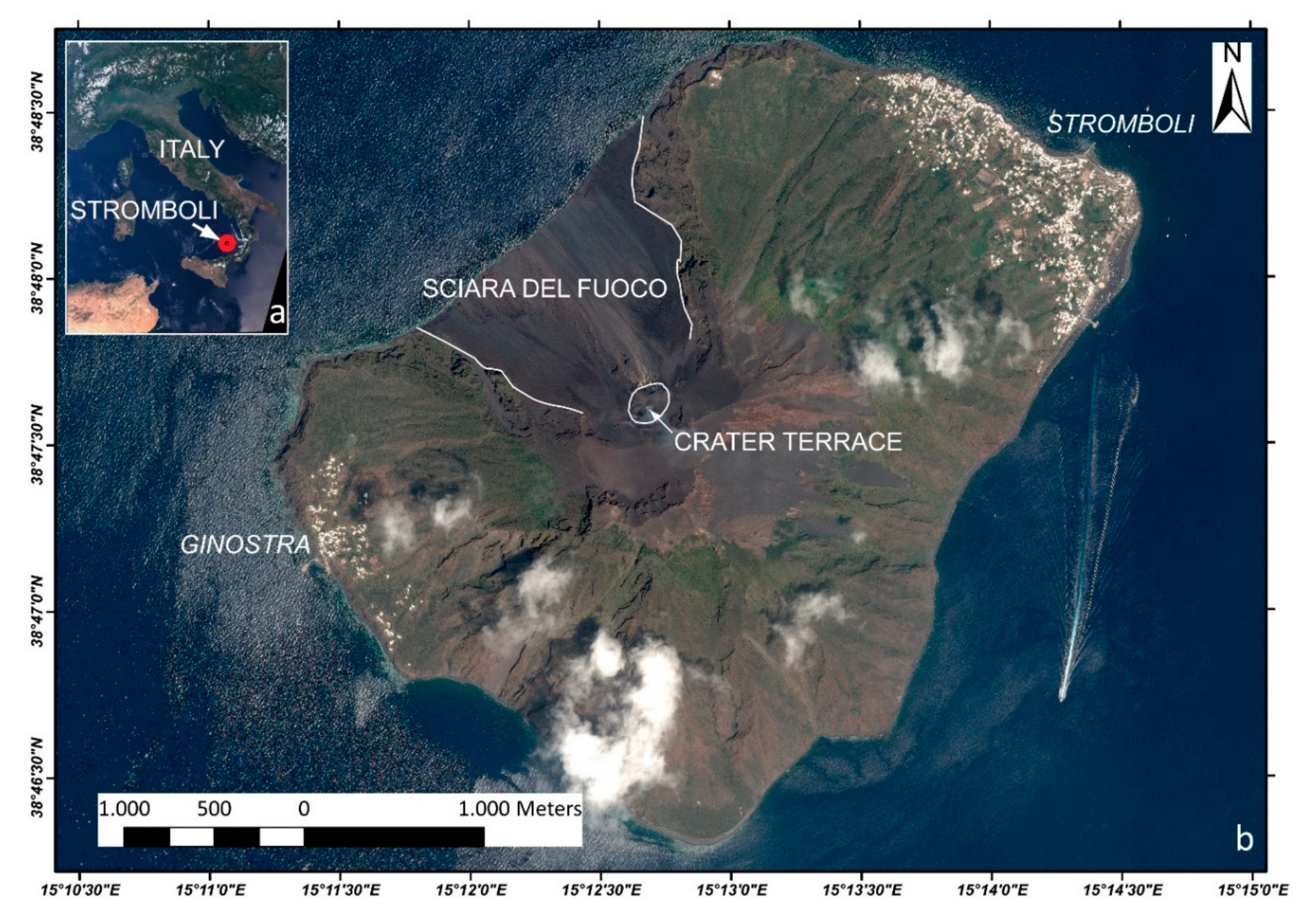
2.1. Study Area
2.2. Geomorphological Mapping
2.3. Topographic Source Data and Methods
2.4. DEMs Co-Registration and Topographic Change Detection
- Preliminary DEMs comparison: Two DEMs were compared, and their differences were visualized in map in order to detect the areas that were affected by topographic changes due to volcanic activity and/or natural phenomena as well as the distribution of errors outside the areas affected by real changes.
- Detection of target areas and initial RMS displacement calculation: A given number of areas without relevant natural changes around the region of interest, in this case the Sciara del Fuoco scar, were selected for DEMs coregistration and the initial RMS displacement between the two DEMs calculated for these areas.
- Calculation of the minimization parameters: The minimization algorithm based on MINUIT was launched and the minimization parameters, and the final RMS displacement was calculated for the target areas.
- DEMs coregistration: Minimization parameters were used for coregistering one DEM (slave) on the DEM previously chosen as a reference (master).
- Selection of independent areas and calculation of RMS displacement error : Since the areas used for calculating were targeted by the minimization process, could not be used for the error calculations of thicknesses and volumes. Independent areas, not affected by natural changes and that were as close as possible to the region of interest, were used to check the residual mismatching between the two DEMs. Note that in this case, the resulting RMS displacement error was the RMS residuals (in elevation) between one DEM and another arbitrary one chosen as a reference, rather than a true absolute error [68].
3. Results
3.1. DEMs Comparison
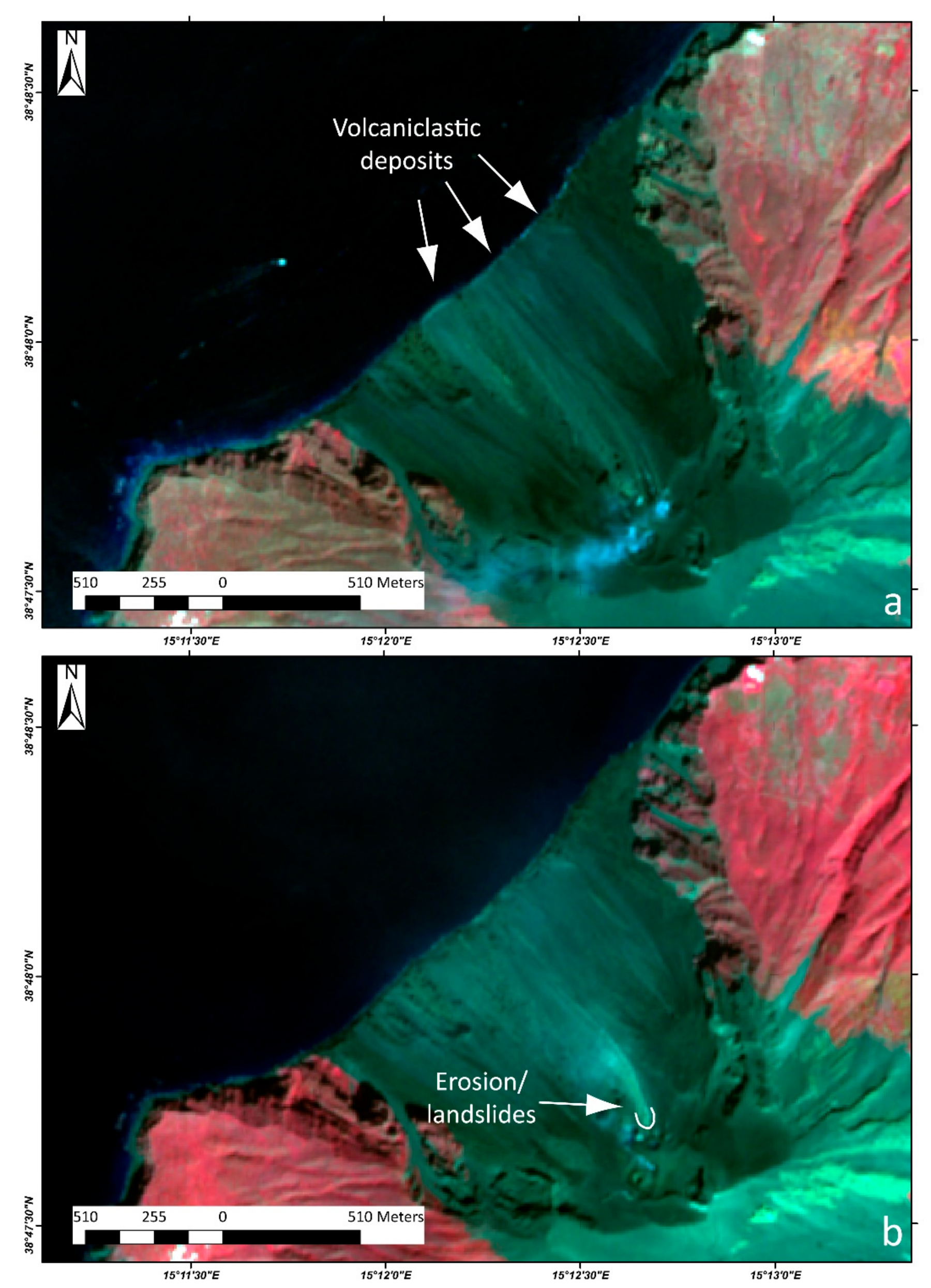
3.2. Morphological Changes
4. Discussion
5. Conclusions
Supplementary Materials
Author Contributions
Funding
Acknowledgments
Conflicts of Interest
References
- Thouret, J.C. Volcanic geomorphology—An overview. Earth-Sci. Rev. 1999, 47, 95–131. [Google Scholar] [CrossRef]
- Schaefer, L.N.; Di Traglia, F.; Chaussard, E.; Lu, Z.; Nolesini, T.; Casagli, N. Monitoring volcano slope instability with Synthetic Aperture Radar: A review and new data from Pacaya (Guatemala) and Stromboli (Italy) volcanoes. Earth-Sci. Rev. 2019, 192, 236–257. [Google Scholar] [CrossRef]
- Wadge, G.; Francis, P.W.; Ramirez, C.F. The Socompa collapse and avalanche event. J. Volcanol. Geotherm. Res. 1995, 66, 309–336. [Google Scholar] [CrossRef]
- Chorowicz, J.; Deffontaines, B.; Huaman-Rodrigo, D.; Guillande, R.; Leguern, F.; Thouret, J.C. SPOT satellite monitoring of the eruption of Nevado Sabancaya volcano (Southern Peru). Remote Sens. Environ. 1992, 42, 43–49. [Google Scholar] [CrossRef]
- Chorowicz, J.; Lopez, E.; Garcia, F.; Parrot, J.F.; Rudant, J.P.; Vinluan, R. Keys to analyze active lahars from Pinatubo on SAR ERS imagery. Remote Sens. Environ. 1997, 62, 20–29. [Google Scholar] [CrossRef]
- Kerle, N.; Froger, J.L.; Oppenheimer, C.; Vries, B.V.W.D. Remote sensing of the 1998 mudflow at Casita volcano, Nicaragua. Int. J. Remote Sens. 2003, 24, 4791–4816. [Google Scholar] [CrossRef]
- Torres, R.; Mouginis-Mark, P.; Self, S.; Garbeil, H.; Kallianpur, K.; Quiambao, R. Monitoring the evolution of the Pasig–Potrero alluvial fan, Pinatubo Volcano, using a decade of remote sensing data. J. Volcanol. Geotherm. Res. 2004, 138, 371–392. [Google Scholar] [CrossRef]
- Ernst, G.G.J.; Kervyn, M.; Teeuw, R.M. Advances in the remote sensing of volcanic activity and hazards, with special consideration to applications in developing countries. Int. J. Remote Sens. 2008, 29, 6687–6723. [Google Scholar] [CrossRef]
- Canisius, F.; Honda, K.; Tokunaga, M. Updating geomorphic features of watersheds and their boundaries in hazardous areas using satellite synthetic aperture radar. Int. J. Remote Sens. 2009, 30, 5919–5933. [Google Scholar] [CrossRef]
- Thouret, J.C.; Gupta, A.; Lube, G.; Liew, S.C.; Cronin, S.J. The 2006 pyroclastic deposits of Merapi Volcano, Java, Indonesia: High-spatial resolution IKONOS images and complementary ground based observations. Remote Sens. Environ. 2010, 114, 1949–1967. [Google Scholar] [CrossRef]
- Wadge, G.; Cole, P.; Stinton, A.; Komorowski, J.C.; Stewart, R.; Toombs, A.C.; Legendre, Y. Rapid topographic change measured by high-resolution satellite radar at Soufriere Hills Volcano, Montserrat, 2008–2010. J. Volcanol. Geotherm. Res. 2011, 199, 142–152. [Google Scholar] [CrossRef]
- Dietterich, H.R.; Poland, M.P.; Schmidt, D.A.; Cashman, K.V.; Sherrod, D.R.; Espinosa, A.T. Tracking lava flow emplacement on the east rift zone of Kīlauea, Hawai ‘i, with synthetic aperture radar coherence. Geochem. Geophys. Geosyst. 2012, 13, Q05001. [Google Scholar] [CrossRef]
- Ebmeier, S.K.; Biggs, J.; Mather, T.A.; Elliott, J.R.; Wadge, G.; Amelung, F. Measuring large topographic change with InSAR: Lava thicknesses, extrusion rate and subsidence rate at Santiaguito volcano, Guatemala. Earth Planet. Sci. Lett. 2012, 335, 216–225. [Google Scholar] [CrossRef] [Green Version]
- Ebmeier, S.K.; Biggs, J.; Muller, C.; Avard, G. Thin-skinned mass-wasting responsible for widespread deformation at Arenal volcano. Front. Earth Sci. 2014, 2, 35. [Google Scholar] [CrossRef] [Green Version]
- Kassouk, Z.; Thouret, J.C.; Gupta, A.; Solikhin, A.; Liew, S.C. Object-oriented classification of a high-spatial resolution SPOT5 image for mapping geology and landforms of active volcanoes: Semeru case study, Indonesia. Geomorphology 2014, 221, 18–33. [Google Scholar] [CrossRef]
- Solikhin, A.; Pinel, V.; Vandemeulebrouck, J.; Thouret, J.C.; Hendrasto, M. Mapping the 2010 Merapi pyroclastic deposits using dual-polarization Synthetic Aperture Radar (SAR) data. Remote Sens. Environ. 2015, 158, 180–192. [Google Scholar] [CrossRef]
- Solikhin, A.; Thouret, J.C.; Liew, S.C.; Gupta, A.; Sayudi, D.S.; Oehler, J.F.; Kassouk, Z. High-spatial-resolution imagery helps map deposits of the large (VEI 4) 2010 Merapi Volcano eruption and their impact. Bull. Volcanol. 2015, 77, 20. [Google Scholar] [CrossRef]
- Thouret, J.C.; Kassouk, Z.; Gupta, A.; Liew, S.C.; Solikhin, A. Tracing the evolution of 2010 Merapi volcanic deposits (Indonesia) based on object-oriented classification and analysis of multi-temporal, very high resolution images. Remote Sens. Environ. 2015, 170, 350–371. [Google Scholar] [CrossRef]
- Arnold, D.W.D.; Biggs, J.; Wadge, G.; Ebmeier, S.K.; Odbert, H.M.; Poland, M.P. Dome growth, collapse, and valley fill at Soufrière Hills Volcano, Montserrat, from 1995 to 2013: Contributions from satellite radar measurements of topographic change. Geosphere 2016, 12, 1300–1315. [Google Scholar] [CrossRef] [Green Version]
- Arnold, D.W.D.; Biggs, J.; Anderson, K.; Vallejo Vargas, S.; Wadge, G.; Ebmeier, S.K.; Naranjo, M.F.; Mothes, P. Decaying Lava Extrusion Rate at El Reventador Volcano, Ecuador, Measured Using High-Resolution Satellite Radar. J. Geophys. Res.: Solid Earth 2017, 122, 9966–9988. [Google Scholar] [CrossRef] [Green Version]
- Chaussard, E. A low-cost method applicable worldwide for remotely mapping lava dome growth. J. Volcanol. Geotherm. Res. 2017, 341, 33–41. [Google Scholar] [CrossRef]
- Arnold, D.W.D.; Biggs, J.; Wadge, G.; Mothes, P. Using satellite radar amplitude imaging for monitoring syn-eruptive changes in surface morphology at an ice-capped stratovolcano. Remote Sens. Environ. 2018, 209, 480–488. [Google Scholar] [CrossRef] [Green Version]
- Di Traglia, F.; Nolesini, T.; Ciampalini, A.; Solari, L.; Frodella, W.; Bellotti, F.; Fumagalli, A.; De Rosa, G.; Casagli, N. Tracking morphological changes and slope instability using spaceborne and ground-based SAR data. Geomorphology 2018, 300, 95–112. [Google Scholar] [CrossRef]
- Coltelli, M.; Proietti, C.; Branca, S.; Marsella, M.; Andronico, D.; Lodato, L. Analysis of the 2001 lava flow eruption of Mt. Etna from three-dimensional mapping. J. Geophys. Res.: Earth Surf. 2007, 112, F02029. [Google Scholar] [CrossRef]
- Baldi, P.; Fabris, M.; Marsella, M.; Monticelli, R. Monitoring the morphological evolution of the Sciara del Fuoco during the 2002–2003 Stromboli eruption using multi-temporal photogrammetry. Isprs J. Photogramm. Remote Sens. 2005, 59, 199–211. [Google Scholar] [CrossRef]
- Neri, M.; Lanzafame, G. Structural features of the 2007 Stromboli eruption. J. Volcanol. Geotherm. Res. 2009, 182, 137–144. [Google Scholar] [CrossRef]
- Baldi, P.; Coltelli, M.; Fabris, M.; Marsella, M.; Tommasi, P. High precision photogrammetry for monitoring the evolution of the NW flank of Stromboli volcano during and after the 2002–2003 eruption. Bull. Volcanol. 2008, 70, 703–715. [Google Scholar] [CrossRef]
- Marsella, M.; Proietti, C.; Sonnessa, A.; Coltelli, M.; Tommasi, P.; Bernardo, E. The evolution of the Sciara del Fuoco subaerial slope during the 2007 Stromboli eruption: Relation between deformation processes and effusive activity. J. Volcanol. Geotherm. Res. 2009, 182, 201–213. [Google Scholar] [CrossRef]
- Favalli, M.; Karátson, D.; Mazzarini, F.; Pareschi, M.T.; Boschi, E. Morphometry of scoria cones located on a volcano flank: A case study from Mt. Etna (Italy), based on high-resolution LiDAR data. J. Volcanol. Geotherm. Res. 2009, 186, 320–330. [Google Scholar] [CrossRef]
- Favalli, M.; Fornaciai, A.; Mazzarini, F.; Harris, A.; Neri, M.; Behncke, B.; Pareschi, M.T.; Tarquini, S.; Boschi, E. Evolution of an active lava flow field using a multitemporal LIDAR acquisition. J. Geophys. Res.: Solid Earth 2010, 115, B11203. [Google Scholar] [CrossRef] [Green Version]
- Fornaciai, A.; Behncke, B.; Favalli, M.; Neri, M.; Tarquini, S.; Boschi, E. Detecting short-term evolution of Etnean scoria cones: A LIDAR-based approach. Bull. Volcanol. 2010, 72, 1209–1222. [Google Scholar] [CrossRef]
- Marsella, M.; Baldi, P.; Coltelli, M.; Fabris, M. The morphological evolution of the Sciara del Fuoco since 1868: Reconstructing the effusive activity at Stromboli volcano. Bull. Volcanol. 2012, 74, 231–248. [Google Scholar] [CrossRef]
- Behncke, B.; Branca, S.; Corsaro, R.A.; De Beni, E.; Miraglia, L.; Proietti, C. The 2011–2012 summit activity of Mount Etna: Birth, growth and products of the new SE crater. J. Volcanol. Geotherm. Res. 2014, 270, 10–21. [Google Scholar] [CrossRef]
- De Beni, E.; Behncke, B.; Branca, S.; Nicolosi, I.; Carluccio, R.; Caracciolo, F.A.; Chiappini, M. The continuing story of Etna’s New Southeast Crater (2012–2014): Evolution and volume calculations based on field surveys and aerophotogrammetry. J. Volcanol. Geotherm. Res. 2015, 303, 175–186. [Google Scholar] [CrossRef]
- Bagnardi, M.; González, P.J.; Hooper, A. High-resolution digital elevation model from tri-stereo PLÉIADES-1 satellite imagery for lava flow volume estimates at Fogo Volcano. Geophys. Res. Lett. 2016, 43, 6267–6275. [Google Scholar] [CrossRef] [Green Version]
- Behncke, B.; Fornaciai, A.; Neri, M.; Favalli, M.; Ganci, G.; Mazzarini, F. Lidar surveys reveal eruptive volumes and rates at Etna, 2007–2010. Geophys. Res. Lett. 2016, 43, 4270–4278. [Google Scholar] [CrossRef] [Green Version]
- Roberti, G.; Ward, B.; de Vries, B.V.W.; Friele, P.; Perotti, L.; Clague, J.J.; Giardino, M. Precursory slope distress prior to the 2010 Mount Meager landslide, British Columbia. Landslides 2018, 15, 1–11. [Google Scholar] [CrossRef]
- Roberti, G.; Friele, P.; de Vries, B.V.W.; Ward, B.; Clague, J.J.; Perotti, L.; Giardino, M. Rheological evolution of the Mount Meager 2010 debris avalanche, southwestern British Columbia. Geosphere 2017, 13, 369–390. [Google Scholar] [CrossRef] [Green Version]
- Richter, N.; Favalli, M.; de Zeeuw-van Dalfsen, E.; Fornaciai, A.; Fernandes, R.M.D.S.; Pérez, N.M.; Levy, J.; Silva Victoria, S.; Walter, T.R. Lava flow hazard at Fogo Volcano, Cabo Verde, before and after the 2014–2015 eruption. Nat. Hazards Earth Syst. Sci. 2016, 16, 1925. [Google Scholar] [CrossRef] [Green Version]
- Naranjo, M.F.; Ebmeier, S.K.; Vallejo, S.; Ramón, P.; Mothes, P.; Biggs, J.; Herrera, F. Mapping and measuring lava volumes from 2002 to 2009 at El Reventador Volcano, Ecuador, from field measurements and satellite remote sensing. J. Appl. Volcanol. 2016, 5, 8. [Google Scholar] [CrossRef] [Green Version]
- Di Traglia, F.; Calvari, S.; D’Auria, L.; Nolesini, T.; Bonaccorso, A.; Fornaciai, A.; Esposito, A.; Cristaldi, A.; Favalli, M.; Casagli, N. The 2014 Effusive Eruption at Stromboli: New Insights from In Situ and Remote-Sensing Measurements. Remote Sens. 2018, 10, 2035. [Google Scholar] [CrossRef] [Green Version]
- Pedersen, G.B.M.; Belart, J.M.C.; Magnússon, E.; Vilmundardóttir, O.K.; Kizel, F.; Sigurmundsson, F.S.; Gísladóttir, G.; Benediktsson, J.A. Hekla volcano, Iceland, in the 20th century: Lava volumes, production rates, and effusion rates. Geophys. Res. Lett. 2018, 45, 1805–1813. [Google Scholar] [CrossRef] [Green Version]
- Intrieri, E.; Di Traglia, F.; Del Ventisette, C.; Gigli, G.; Mugnai, F.; Luzi, G.; Casagli, N. Flank instability of Stromboli volcano (Aeolian Islands, Southern Italy): Integration of GB-InSAR and geomorphological observations. Geomorphology 2013, 201, 60–69. [Google Scholar] [CrossRef]
- Calvari, S.; Bonaccorso, A.; Madonia, P.; Neri, M.; Liuzzo, M.; Salerno, G.G.; Behncke, B.; Caltabiano, T.; Cristaldi, A.; Giuffrida, G.; et al. Major eruptive style changes induced by structural modifications of a shallow conduit system: The 2007–2012 Stromboli case. Bull. Volcanol. 2014, 76, 841. [Google Scholar] [CrossRef]
- Romagnoli, C.; Kokelaar, P.; Casalbore, D.; Chiocci, F.L. Lateral collapses and active sedimentary processes on the northwestern flank of Stromboli volcano, Italy. Mar. Geol. 2009, 265, 101–119. [Google Scholar] [CrossRef]
- Tibaldi, A. Multiple sector collapses at Stromboli volcano, Italy: How they work. Bull. Volcanol. 2001, 63, 112–125. [Google Scholar] [CrossRef]
- Di Roberto, A.; Rosi, M.; Bertagnini, A.; Marani, M.P.; Gamberi, F. Distal turbidites and tsunamigenic landslides of Stromboli volcano (Aeolian Islands, Italy). In Submarine Mass Movements and Their Consequences; Springer: Dordrecht, The Netherlands, 2010; pp. 719–731. [Google Scholar]
- Kokelaar, P.; Romagnoli, C. Sector collapse, sedimentation and clast population evolution at an active island-arc volcano: Stromboli, Italy. Bull. Volcanol. 1995, 57, 240–262. [Google Scholar] [CrossRef]
- Rotonda, T.; Tommasi, P.; Boldini, D. Geomechanical characterization of the volcaniclastic material involved in the 2002 landslides at Stromboli. J. Geotech. Geoenviron. Eng. 2009, 136, 389–401. [Google Scholar] [CrossRef]
- Nolesini, T.; Di Traglia, F.; Del Ventisette, C.; Moretti, S.; Casagli, N. Deformations and slope instability on Stromboli volcano: Integration of GBInSAR data and analog modeling. Geomorphology 2013, 180, 242–254. [Google Scholar] [CrossRef]
- Calvari, S.; Spampinato, L.; Lodato, L.; Harris, A.J.; Patrick, M.R.; Dehn, J.; Burton, M.; Andronico, D. Chronology and complex volcanic processes during the 2002–2003 flank eruption at Stromboli volcano (Italy) reconstructed from direct observations and surveys with a handheld thermal camera. J. Geophys. Res.: Solid Earth 2005, 110, B02201. [Google Scholar] [CrossRef] [Green Version]
- Blackburn, E.A.; Wilson, L.; Sparks, R.J. Mechanisms and dynamics of strombolian activity. J. Geol. Soc. 1976, 132, 429–440. [Google Scholar] [CrossRef]
- Coppola, D.; Piscopo, D.; Laiolo, M.; Cigolini, C.; Delle Donne, D.; Ripepe, M. Radiative heat power at Stromboli volcano during 2000–2011: Twelve years of MODIS observations. J. Volcanol. Geotherm. Res. 2012, 215, 48–60. [Google Scholar] [CrossRef] [Green Version]
- Di Traglia, F.; Cauchie, L.; Casagli, N.; Saccorotti, G. Decrypting geophysical signals at Stromboli Volcano (Italy): Integration of seismic and Ground-Based InSAR displacement data. Geophys. Res. Lett. 2014, 41, 2753–2761. [Google Scholar] [CrossRef]
- Di Traglia, F.; Nolesini, T.; Intrieri, E.; Mugnai, F.; Leva, D.; Rosi, M.; Casagli, N. Review of ten years of volcano deformations recorded by the ground-based InSAR monitoring system at Stromboli volcano: A tool to mitigate volcano flank dynamics and intense volcanic activity. Earth-Sci. Rev. 2014, 139, 317–335. [Google Scholar] [CrossRef] [Green Version]
- Di Traglia, F.; Intrieri, E.; Nolesini, T.; Bardi, F.; Del Ventisette, C.; Ferrigno, F.; Frangioni, S.; Frodella, W.; Gigli, G.; Lotti, A.; et al. The Ground-Based InSAR monitoring system at Stromboli volcano: Linking changes in displacement rate and intensity of persistent volcanic activity. Bull. Volcanol. 2014, 76, 786. [Google Scholar] [CrossRef]
- Di Traglia, F.; Battaglia, M.; Nolesini, T.; Lagomarsino, D.; Casagli, N. Shifts in the eruptive styles at Stromboli in 2010–2014 revealed by ground-based InSAR data. Sci. Rep. 2015, 5, 13569. [Google Scholar] [CrossRef] [PubMed] [Green Version]
- Rizzo, A.L.; Federico, C.; Inguaggiato, S.; Sollami, A.; Tantillo, M.; Vita, F.; Bellomo, S.; Longo, M.; Grassa, F.; Liuzzo, M. The 2014 effusive eruption at Stromboli volcano (Italy): Inferences from soil CO2 flux and 3He/4He ratio in thermal waters. Geophys. Res. Lett. 2015, 42, 2235–2243. [Google Scholar] [CrossRef]
- Liotta, M.; Rizzo, A.L.; Barnes, J.D.; D’Auria, L.; Martelli, M.; Bobrowski, N.; Wittmer, J. Chlorine isotope composition of volcanic rocks and gases at Stromboli volcano (Aeolian Islands, Italy): Inferences on magmatic degassing prior to 2014 eruption. J. Volcanol. Geotherm. Res. 2017, 336, 168–178. [Google Scholar] [CrossRef]
- Di Traglia, F.; Nolesini, T.; Solari, L.; Ciampalini, A.; Frodella, W.; Steri, D.; Allotta, B.; Rindi, A.; Marini, L.; Monni, N.; et al. Lava delta deformation as a proxy for submarine slope instability. Earth Planet. Sci. Lett. 2018, 488, 46–58. [Google Scholar] [CrossRef]
- Giudicepietro, F.; Calvari, S.; Alparone, S.; Bianco, F.; Bonaccorso, A.; Bruno, V.; Caputo, T.; Cristaldi, A.; D’Auria, L.; De Cesare, W.; et al. Integration of Ground-Based Remote-Sensing and In Situ Multidisciplinary Monitoring Data to Analyze the Eruptive Activity of Stromboli Volcano in 2017–2018. Remote Sens. 2019, 11, 1813. [Google Scholar] [CrossRef] [Green Version]
- Di Traglia, F.; Bartolini, S.; Artesi, E.; Nolesini, T.; Ciampalini, A.; Lagomarsino, D.; Martí, J.; Casagli, N. Susceptibility of intrusion-related landslides at volcanic islands: The Stromboli case study. Landslides 2018, 15, 21–29. [Google Scholar] [CrossRef] [Green Version]
- Nave, R.; Isaia, R.; Vilardo, G.; Barclay, J. Re-assessing volcanic hazard maps for improving volcanic risk communication: Application to Stromboli Island, Italy. J. Maps 2010, 6, 260–269. [Google Scholar] [CrossRef] [Green Version]
- Fornaciai, A.; Favalli, M.; Nannipieri, L. Numerical simulation of the tsunamis generated by the Sciara del Fuoco landslides (Stromboli Island, Italy). Sci. Rep. 2019, 9, 1–12. [Google Scholar] [CrossRef] [PubMed] [Green Version]
- Salvatici, T.; Di Roberto, A.; Di Traglia, F.; Bisson, M.; Morelli, S.; Fidolini, F.; Bertagnini, A.; Pompilio, M.; Hungr, O.; Casagli, N. From hot rocks to glowing avalanches: Numerical modelling of gravity-induced pyroclastic density currents and hazard maps at the Stromboli Volcano (Italy). Geomorphology 2016, 273, 93–106. [Google Scholar] [CrossRef] [Green Version]
- Zhou, Y.; Parsons, B.; Elliott, J.R.; Barisin, I.; Walker, R.T. Assessing the ability of PLÉIADES stereo imagery to determine height changes in earthquakes: A case study for the El Mayor-Cucapah epicentral area. J. Geophys. Res.: Solid Earth 2015, 120, 8793–8808. [Google Scholar] [CrossRef] [Green Version]
- Kolzenburg, S.; Favalli, M.; Fornaciai, A.; Isola, I.; Harris, A.J.L.; Nannipieri, L.; Giordano, D. Rapid updating and improvement of airborne LIDAR DEMs through ground-based SfM 3-D modeling of volcanic features. Ieee Trans. Geosci. Remote Sens. 2016, 54, 6687–6699. [Google Scholar] [CrossRef]
- Favalli, M.; Fornaciai, A.; Nannipieri, L.; Harris, A.; Calvari, S.; Lormand, C. UAV-based remote sensing surveys of lava flow fields: A case study from Etna’s 1974 channel-fed lava flows. Bull. Volcanol. 2018, 80, 29. [Google Scholar] [CrossRef]
- James, F.; Roos, M. MINUIT: A system for function minimization and analysis of the parameter errors and corrections. Comput. Phys. Commun. 1975, 10, 343–367. [Google Scholar] [CrossRef]
- Fornaciai, A.; Bisson, M.; Landi, P.; Mazzarini, F.; Pareschi, M.T. A LiDAR survey of Stromboli volcano (Italy): Digital elevation model-based geomorphology and intensity analysis. Int. J. Remote Sens. 2010, 31, 3177–3194. [Google Scholar] [CrossRef]
- Favalli, M.; Fornaciai, A. Visualization and comparison of DEM-derived parameters. Application to volcanic areas. Geomorphology 2017, 290, 69–84. [Google Scholar] [CrossRef]
- Yokoyama, R.; Shirasawa, M.; Pike, R.J. Visualizing topography by openness: A new application of image processing to digital elevation models. Photogramm. Eng. Remote Sens. 2002, 68, 257–266. [Google Scholar]
- Karátson, D.; Yepes, J.; Favalli, M.; Rodríguez-Peces, M.J.; Fornaciai, A. Reconstructing eroded paleovolcanoes on Gran Canaria, Canary Islands, using advanced geomorphometry. Geomorphology 2016, 253, 123–134. [Google Scholar] [CrossRef]
- Sofia, G.; Bailly, J.S.; Chehata, N.; Tarolli, P.; Levavasseur, F. Comparison of PLÉIADES and LiDAR digital elevation models for terraces detection in farmlands. Ieee J. Sel. Top. Appl. Earth Obs. Remote Sens. 2016, 9, 1567–1576. [Google Scholar] [CrossRef] [Green Version]
- Poli, D.; Remondino, F.; Angiuli, E.; Agugiaro, G. Evaluation of Pléiades-1A triplet on Trento testfield. Int. Arch. Photogramm. Remote Sens. Spat. Inf. Sci. 2013, 1, 287–292. [Google Scholar] [CrossRef] [Green Version]
- Serrano, E.; Sanjosé, J.J.; Gómez-Gutiérrez, A.; Gómez-Lende, M. Surface movement and cascade processes on debris cones in temperate high mountain (Picos de Europa, northern Spain). Sci. Total. Environ. 2019, 649, 1323–1337. [Google Scholar] [CrossRef] [PubMed]
- Chiocci, F.L.; Romagnoli, C.; Tommasi, P.; Bosman, A. The Stromboli 2002 tsunamigenic submarine slide: Characteristics and possible failure mechanisms. J. Geophys. Res.: Solid Earth 2008, 113, B10102. [Google Scholar] [CrossRef]
- Casalbore, D.; Romagnoli, C.; Chiocci, F.; Frezza, V. Morpho-sedimentary characteristics of the volcaniclastic apron around Stromboli volcano (Italy). Mar. Geol. 2010, 269, 132–148. [Google Scholar] [CrossRef]
- Casalbore, D.; Romagnoli, C.; Bosman, A.; Chiocci, F.L. Potential tsunamigenic landslides at Stromboli Volcano (Italy): Insight from marine DEM analysis. Geomorphology 2011, 126, 42–50. [Google Scholar] [CrossRef]


| Date | Eruptive Activity | Slope Processes | References |
|---|---|---|---|
| March 2010 | Strong explosive event (10 March 2010), ejecta outside the crater, and rheomorphic lava flows to the NEC | [44,53] | |
| May 2010–June 2010 | Strong explosive events, rheomorphic lava flows and intracrateric lava flows | [44,53] | |
| October 2010 | Intracrater lava flow from the SWC vent (19–26 October 2010) | [44,53] | |
| December 2010–January 2011 | Strong explosive events, intense spattering and overflows from the SWC | [44,53] | |
| March 2011 | Strong explosive event (4 March 2011) from the SWC | [44,53] | |
| June 2011–September 2011 | Strong explosive events and two overflows | [44,53,54,55] | |
| February–March 2012 | Strong explosive events (15–16 February 2012, 6 March 2012) | [44,55] | |
| July 2012–August 2012 | Major explosions, intense spattering and overflows | [44] | |
| December 2012–June 2013 | Several lava overflows, strong explosive events and intense spatter activity, as well as a high displacement rate in the crater terrace | Crater-wall rock slide (12 January 2013), frequent rockfall and gravel flows during lava overflows | [44,55,56] |
| December 2013–March 2014 | Strong explosive events, intense spattering, and anomalous degassing | [58,59] | |
| June 2014–November 2014 | Several lava overflows, strong explosive events, intense spatter activity, opening of an ephemeral vent at 650 m a.s.l. (100 below the NEC), and lava flow lasting 3 months | Frequent rockfall and gravel flows during lava overflows and sliding of the NEC debris talus (7 August 2014) | [41,57,58,59] |
| November 2014–September 2016 | Rockfall and gravel flows affecting the 2014 lava field | [2,61] | |
| December 2017–January 2018 | Intense spatter activity and a lava overflow | Frequent rockfall and gravel flows during spatter activity | [2,61] |
| December 2018–January 2019 | Intense spatter activity | Frequent rockfall and gravel flows during spatter activity | This study |
| Volcano | Techniques | References |
|---|---|---|
| Casita (Nicaragua) | Optical images change detection–SAR amplitude change detection | 6 |
| Pinatubo (Philippines) | Optical images change detection | 7 |
| Merapi (Indonesia) | Optical image object-oriented classification | 18 |
| Merapi (Indonesia) | Optical images change detection | 16 |
| Merapi (Indonesia) | Optical image change detection–Topographic change detection | 18 |
| Merapi (Indonesia) | Polarization SAR analysis | 17 |
| Semeru (Indonesia) | Optical image object-oriented classification | 15 |
| Stromboli (Italy) | Topographic change detection (photogrammetry) | 25, 27 |
| Stromboli (Italy) | Topographic change detection (photogrammetry) | 28 |
| Stromboli (Italy) | Topographic change detection (PLÉIADES tri-stereo) | 41 |
| Stromboli (Italy) | SAR amplitude change detection—SAR amplitude texture analysis | 23 |
| Etna (Italy) | Topographic change detection (LiDAR) | 24 |
| Etna (Italy) | Topographic change detection (LiDAR) | 30 |
| Etna (Italy) | Topographic change detection (LiDAR) | 31 |
| Etna (Italy) | Topographic change detection (LiDAR–photogrammetry) | 34 |
| Etna (Italy) | Topographic change detection (LiDAR) | 33 |
| Fogo (Cape Verde) | Topographic change detection (TANDEM-X/PLÉIADES tri-stereo) | 35 |
| Fogo (Cape Verde) | Topographic change detection (photogrammetry–TLS) | 39 |
| Soufriere Hills (Montserrat) | SAR amplitude change detection | 11 |
| Soufriere Hills (Montserrat) | SAR amplitude change detection–SAR topographic change detection | 19 |
| Arenal (Costa Rica) | SAR amplitude change detection | 14 |
| Santiaguito (Guatemala) | SAR topographic change detection | 13 |
| El Renventador (Ecuador) | SAR topographic change detection | 40 |
| El Renventador (Ecuador) | SAR amplitude change detection | 20 |
| Cotopaxi (Ecuador) | SAR amplitude change detection | 22 |
| Hekla (Iceland) | Topographic change detection (photogrammetry) | 42 |
| Kilauea (USA) | SAR coherence | 12 |
| Mount St. Helens (USA) | SAR amplitude change detection | 21 |
| QUICKBIRD | PLÉIADES | |
|---|---|---|
| Acquisition date | 21 March 2008 23 September 2012 | 6 May 2016 26 May 2017 28 August 2017 1 September 2018 3 June 2019 |
| Spatial resolution PAN (m) | 0.7 × 0.7 | 0.5 × 0.5 |
| Spatial resolution MS (m) | 2.5 × 2.5 | 1 × 1 |
| Cloud coverage (%) | < 10 | < 5 |
| Spectral resolution (nm) | ||
| Blue | 450–520 | 450–550 |
| Green | 520–600 | 490–610 |
| Red | 630–690 | 600–720 |
| Near infrared | 760–900 | 750–920 |
| Spatial Resolution (m) | Band Number | SENTINEL-2A | SENTINEL-2B | ||
|---|---|---|---|---|---|
| Central Wavelength (nm) | Bandwidth (nm) | Central Wavelength (nm) | Bandwidth (nm) | ||
| 10 | 2 | 496.6 | 98 | 492.1 | 98 |
| 3 | 560.0 | 45 | 559 | 46 | |
| 4 | 664.5 | 38 | 665 | 39 | |
| 8 | 835.1 | 145 | 833 | 133 | |
| 20 | 5 | 703.9 | 19 | 703.8 | 20 |
| 6 | 740.2 | 18 | 739.1 | 18 | |
| 7 | 782.5 | 28 | 779.7 | 28 | |
| 8a | 864.8 | 33 | 864 | 32 | |
| 11 | 1613.7 | 143 | 1610.4 | 141 | |
| 12 | 2202.4 | 242 | 2185.7 | 238 | |
| 60 | 1 | 443.9 | 27 | 442.3 | 45 |
| 9 | 945.0 | 26 | 943.2 | 27 | |
| 10 | 1373.5 | 75 | 1376.9 | 76 | |
| Images Points Residuals (pixels) | |||||||||
| DATE | 6 May 2016 | 26 May 2017 | 28 August 2017 | ||||||
| X | Y | X | Y | X | Y | ||||
| XY BIASS | −0.0003 | 0.0002 | −0.0006 | 0.0006 | 0.003 | 0.0015 | |||
| XY STANDARD DEVIATION | 0.0834 | 0.0857 | 0.0921 | 0.0892 | 0.1419 | 0.1227 | |||
| XY MAX | 0.2694 | 0.2696 | 0.2198 | 0.2440 | 0.3218 | 0.3472 | |||
| Control Points Residuals (m) | |||||||||
| DATE | 6 May 2016 | 26 May 2017 | 28 August 2017 | ||||||
| X | Y | Z | X | Y | Z | X | Y | Z | |
| XYZ BIASS | 0.7114 | −0.1244 | 0.6461 | 0.2973 | −0.2681 | 0.0525 | 0.1605 | −0.0949 | 0.0042 |
| XYZ STANDARD DEVIATION | 0.7057 | 0.5371 | 2.5056 | 0.2289 | 0.0827 | 1.5554 | 0.1914 | 0.1499 | 0.3856 |
| XYZ MAX | 1.5439 | 1.1412 | 4.9776 | 0.5758 | 0.3909 | 3,0559 | 0.4578 | 0.2970 | 0.6948 |
| Images Points Residuals (pixels) | |||||||||
| DATE | 1 September 2018 | 13 June 2019 | |||||||
| X | Y | X | Y | X | Y | ||||
| XY BIASS | 0.0002 | 0.0009 | 0.0002 | 0.0009 | 0.0002 | 0.0009 | |||
| XY STANDARD DEVIATION | 0.1341 | 0.1297 | 0.1341 | 0.1297 | 0.1341 | 0.1297 | |||
| XY MAX | 0.4045 | 0.3841 | 0.4045 | 0.3841 | 0.4045 | 0.3841 | |||
| Control Points Residuals (m) | |||||||||
| DATE | 1 September 2018 | 13 June 2019 | |||||||
| X | Y | X | Y | X | Y | ||||
| XYZ BIASS | 0.0099 | −0.0049 | 0.0099 | −0.0049 | 0.0099 | −0.0049 | |||
| XYZ STANDARD DEVIATION | 0.193792 | 0.1519 | 0.193792 | 0.1519 | 0.193792 | 0.1519 | |||
| XYZ MAX | 0.374875 | 0.2606 | 0.374875 | 0.2606 | 0.374875 | 0.2606 | |||
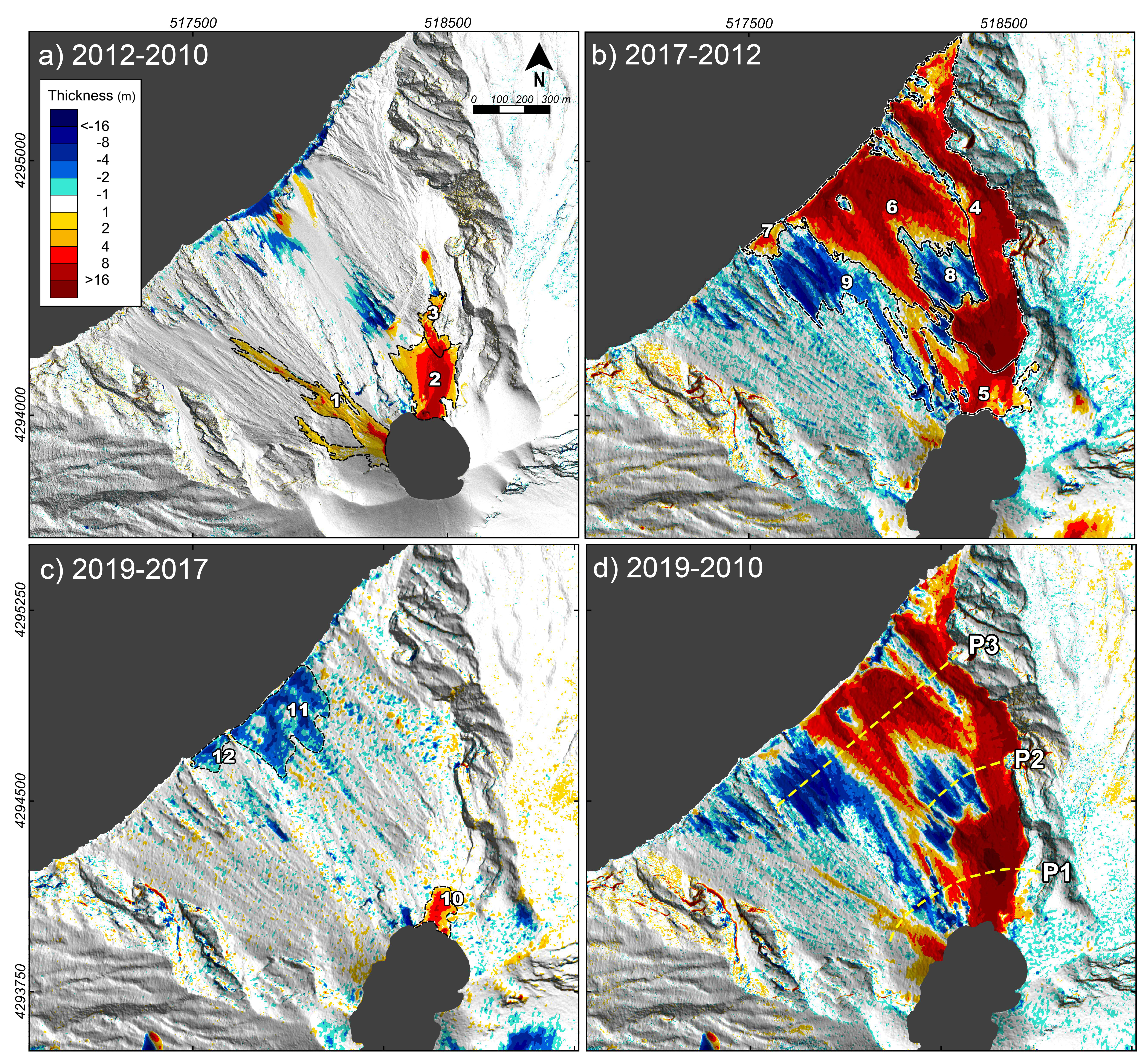
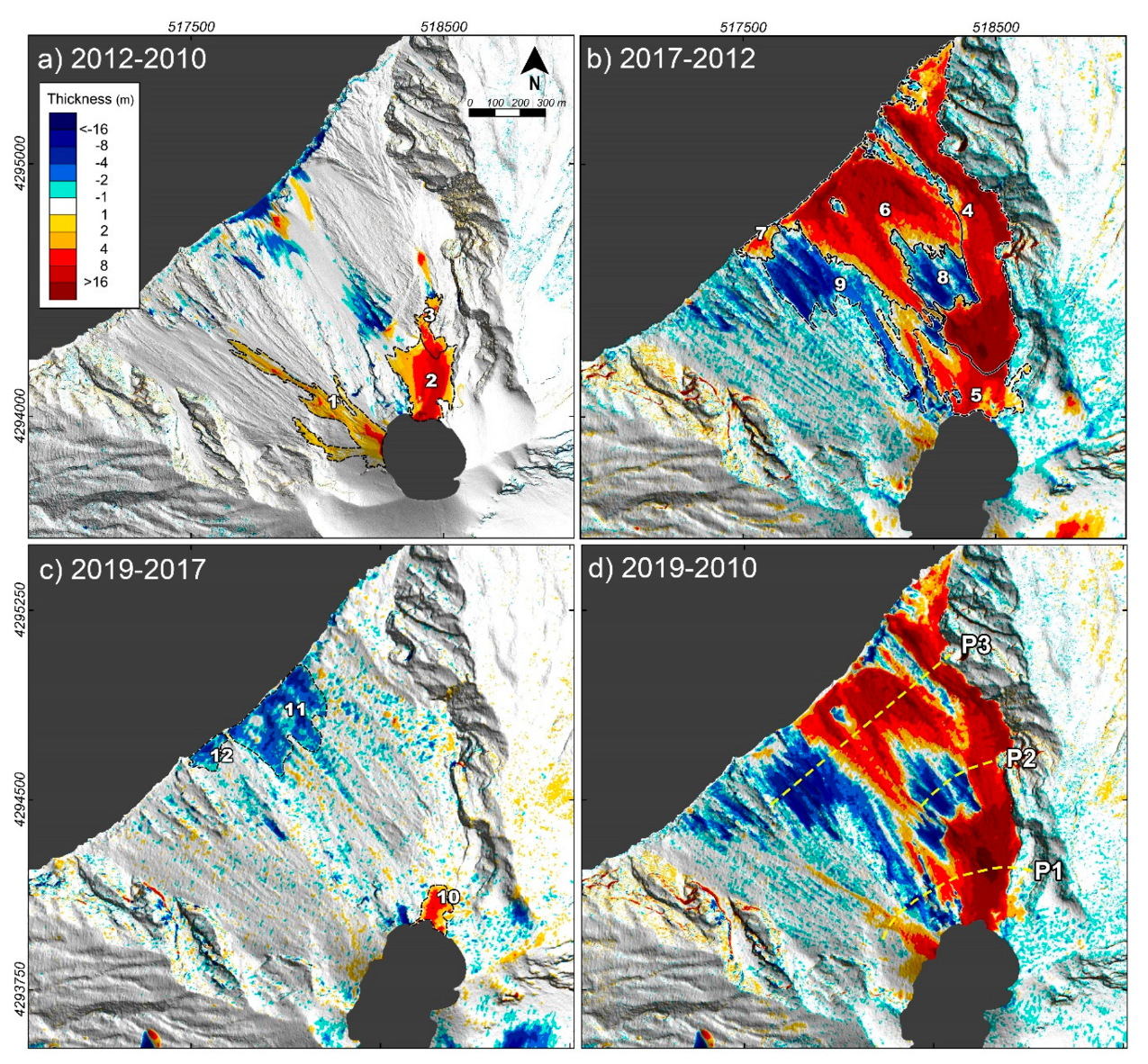
| Time Interval | Sector | Description | Area (× 103 m2) | Volume (× 106 m3) | Mean Thickness (m) | |
|---|---|---|---|---|---|---|
| July 2010–May 2012 | 1 | December 2010 overflow | 63.817 | 0.118 ± 0.022 | 1.850 | 0.350 |
| 2 | NEC debris talus | 52.927 | 0.289 ± 0.019 | 5.465 | 0.350 | |
| 3 | August 2011 overflow | 14.183 | 0.055 ± 0.005 | 3.870 | 0.350 | |
| May 2012–May 2017 | 4 | 2014 lava flow field | 225.399 | 2.697 ± 0.190 | 11.964 | 0.845 |
| 5 | NEC debris talus | 70.189 | 0.396 ± 0.059 | 5.636 | 0.845 | |
| 6 | Volcanoclastic wedge | 242.682 | 1.747 ± 0.205 | 7.199 | 0.845 | |
| 7 | Deposition | 12.064 | 0.031 ± 0.010 | 2.652 | 0.845 | |
| 8 | Erosion | 52.017 | −0.153 ± 0.044 | −2.948 | 0.845 | |
| 9 | Erosion | 122.655 | −0.425 ± 0.104 | −3.469 | 0.845 | |
| June 2019–May 2017 | 10 | NEC debris talus | 15.639 | 0.061 ± 0.008 | 3.900 | 0.528 |
| 11 | Erosion | 84.739 | −0.214 ± 0.045 | −2.524 | 0.528 | |
| 12 | Erosion | 11.962 | −0.027 ± 0.006 | −2.251 | 0.528 |
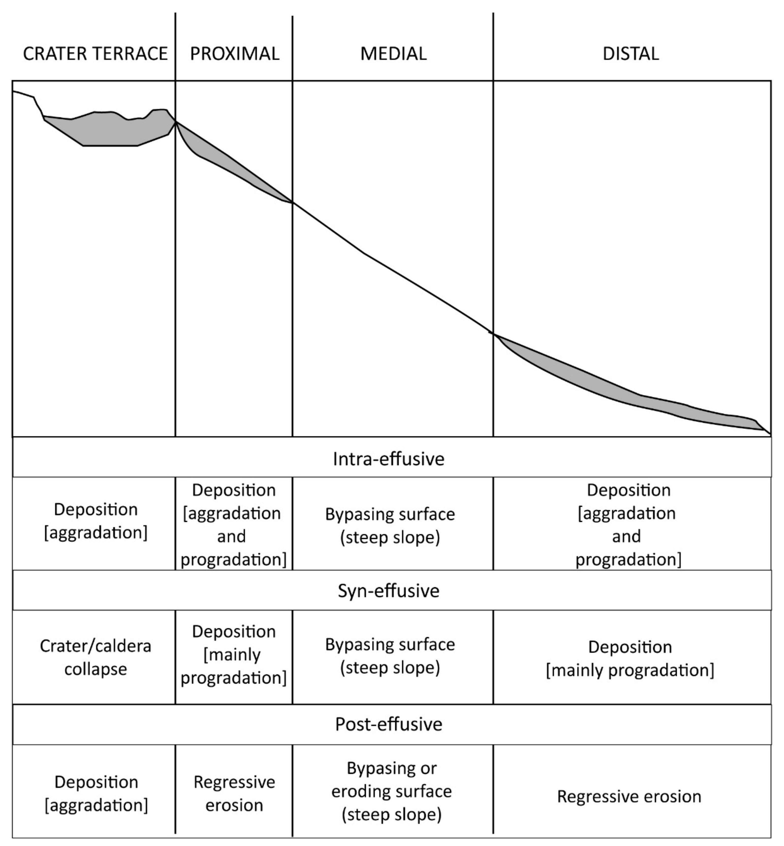
| Crater Terrace | Proximal | Medial | Distal | |
|---|---|---|---|---|
| Landform (erosion and mass-wasting) |
|
|
|
|
| Landform (sedimentation) |
|
|
|
|
| Deposits |
|
|
|
|
| Processes (depletion) |
|
|
|
|
| Processes (accumulation) |
|
|
|
|
© 2020 by the authors. Licensee MDPI, Basel, Switzerland. This article is an open access article distributed under the terms and conditions of the Creative Commons Attribution (CC BY) license (http://creativecommons.org/licenses/by/4.0/).
Share and Cite
Di Traglia, F.; Fornaciai, A.; Favalli, M.; Nolesini, T.; Casagli, N. Catching Geomorphological Response to Volcanic Activity on Steep Slope Volcanoes Using Multi-Platform Remote Sensing. Remote Sens. 2020, 12, 438. https://0-doi-org.brum.beds.ac.uk/10.3390/rs12030438
Di Traglia F, Fornaciai A, Favalli M, Nolesini T, Casagli N. Catching Geomorphological Response to Volcanic Activity on Steep Slope Volcanoes Using Multi-Platform Remote Sensing. Remote Sensing. 2020; 12(3):438. https://0-doi-org.brum.beds.ac.uk/10.3390/rs12030438
Chicago/Turabian StyleDi Traglia, Federico, Alessandro Fornaciai, Massimiliano Favalli, Teresa Nolesini, and Nicola Casagli. 2020. "Catching Geomorphological Response to Volcanic Activity on Steep Slope Volcanoes Using Multi-Platform Remote Sensing" Remote Sensing 12, no. 3: 438. https://0-doi-org.brum.beds.ac.uk/10.3390/rs12030438