A New Deep Learning Network for Automatic Bridge Detection from SAR Images Based on Balanced and Attention Mechanism

Abstract

Bridge detection from Synthetic Aperture Radar (SAR) images has very important strategic significance and practical value, but there are still many challenges in end-to-end bridge detection. In this paper, a new deep learning-based network is proposed to identify bridges from SAR images, namely, multi-resolution attention and balance network (MABN). It mainly includes three parts, the attention and balanced feature pyramid (ABFP) network, the region proposal network (RPN), and the classification and regression. First, the ABFP network extracts various features from SAR images, which integrates the ResNeXt backbone network, balanced feature pyramid, and the attention mechanism. Second, extracted features are used by RPN to generate candidate boxes of different resolutions and fused. Furthermore, the candidate boxes are combined with the features extracted by the ABFP network through the region of interest (ROI) pooling strategy. Finally, the detection results of the bridges are produced by the classification and regression module. In addition, intersection over union (IOU) balanced sampling and balanced L1 loss functions are introduced for optimal training of the classification and regression network. In the experiment, TerraSAR data with 3-m resolution and Gaofen-3 data with 1-m resolution are used, and the results are compared with faster R-CNN and SSD. The proposed network has achieved the highest detection precision (P) and average precision (AP) among the three networks, as 0.877 and 0.896, respectively, with the recall rate (RR) as 0.917. Compared with the other two networks, the false alarm targets and missed targets of the proposed network in this paper are greatly reduced, so the precision is greatly improved.

1. Introduction

Synthetic aperture radar (SAR) system is not affected by the weather and light, which can produce images all day and night [1]. This is a tremendous advantage that optical imaging systems cannot offer, but its imaging characteristics are more difficult to understand than optical images (e.g., the speckle noise in SAR images). Therefore, objects detection and classification turn out to be more challenging for SAR images. Meanwhile, with the rapid increase of spaceborne SAR systems [2], airborne SAR systems [3], and unmanned aerial vehicle (UAV) SAR [4] systems, the number of high-resolution SAR images is also growing and becoming more popular, which has brought more opportunities for the widespread application of SAR imaging.

As a key part of urban infrastructures, bridges over water (all bridges to be detected in this article are bridges over water, referred to as bridges) are a significant category of transportation facilities and one of the pivotal hubs of transportation. More importantly, bridges present special characteristics different from other objects in SAR images. Therefore, automatic detection of bridges has always been an important research topic in the field of SAR image object recognition, and has great significance for the application in multiple fields (e.g., military and civil engineering fields), and has been a research hotspot for decades [5]. If bridges can be detected automatically and accurately from large-scale high-resolution SAR images, it will benefit various civilian and military fields (e.g., natural disaster situation assessment based on SAR images and selection of disaster relief paths [6], weapon terminal guidance based on computer vision and target recognition [7]).

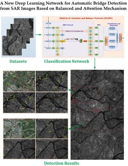
To accomplish this aim, a new deep learning network is proposed, namely, multi-resolution attention and balance network (MABN), which is based on the faster R-CNN [8] structure. First, we develop attention and balanced feature pyramid (ABFP) network to sufficiently extract the features of SAR images. In ABFP, the ResNeXt [9] network is used to produce the feature maps at different scales. Then, balanced feature pyramid [10] and attention mechanism [11] are incurred to further extract the essential features. Second, the region proposal network (RPN) is employed to generate candidate boxes of the targets. Finally, the component of classification and regression is used to accomplish the bridge detection, in which IoU balanced sampling and balanced L1 loss function are employed.

The rest of the paper is arranged as follows. Section 2 introduces the state-of-the-art of the deep learning on objects detection and the development of the bridge detection from SAR images. The proposed bridges detection network is introduced in detail in Section 3, in which, the most important part is the proposed ABFP network. In Section 4, the specific experiments result and analysis of bridge detection are given. Section 5 illustrates the following research. In Section 6, the conclusion is given.

2. State-of-the-Art

With the emergence of more and higher resolution SAR images, SAR images have been more widely used in targets detection. As an important part of the transportation system, bridges play a significant role in people’s lives, disaster relief and national strategies. In recent years, the bridge detection from SAR images has become a research hotspot. Hou et al. [12] proposed an automatic segmentation and recognition algorithm for bridges from high-resolution SAR images, which combined wavelet analysis and image processing. First, wavelet transform was used to pre-filter and denoise the image, and then the improved OSTU threshold method was utilized to detect the edge of the river contour. Finally, the global search algorithm and the rectangular area intermediate axis search algorithm were employed to locate and identify the bridge. Zhang et al. [13] segmented the river by gray threshold and edge detection, utilized wavelet transform to extract linear features of the river, and finally combined the pixel and width information to perform bridge detection. Wang et al. [14] proposed a porosity-based method combined with Canny edge detection to extract water bodies, and detected bridges by considering the universality and geometric characteristics of bridges and water bodies. Sun et al. [15] and Bai et al. [16] adopted similar methods to the above (through edge detectors) to solve the problem of image segmentation, and then the bridge detection from SAR images was achieved. Song et al. [17], Chen et al. [18], Chang et al. [19], and Wang et al. [20] all used Constant False-Alarm Rate (CFAR) algorithm for bridges detection. Huang et al. [21] first extracted the primal sketch features of the image, and then defined the membership function based on the bridge’s geometric information and scene semantic information to calculate and identify bridges. Wu et al. [22] proposed a novel object detection framework, namely, optical remote sensing imagery detector (ORSIm detector), which integrated spatial-frequency channel feature (SFCF), fast image pyramid estimation, and ensemble classifier learning. It achieved better detection accuracy with enhanced reliability. Though it was used in optical remote sensing images, we can also learn much from which and apply them to SAR images.

The above algorithms of bridge extraction all rely on traditional image processing techniques. There are some common problems, such as low robustness or low degree of automation for bridge detection under the complex background of large-scale SAR images, and they cannot achieve high-precision and fail to provide end-to-end detection. Since deep learning was proposed in 2006 [23], it has been widely used in the field of target detection, providing an appealing solution for the intelligent detection of bridges from SAR images.

The target detection algorithms based on deep learning can be mainly divided into two categories, namely the two-stage method and one-stage method. The two-stage method divides the whole detecting process into two stages. First, candidate boxes are extracted in advance according to the position of the target in the image, and then classification and regression are performed to generate the detection results. The typical algorithms mainly include R-CNN [10], fast R-CNN [24], faster R-CNN [25], and mask R-CNN [26]. R-CNN used the selective search algorithm to generate about 2000 candidate boxes in the image, and then utilized convolutional neural networks (CNN) to extract fixed-length feature vectors for each candidate box, and finally used support vector machine (SVM) for target classification and regression. Fast R-CNN added region of interest (ROI) pooling on the basis of R-CNN, which could convert the inputted feature map with any size into a feature representation with a specific size, and uniformly learn classification loss and border regression loss. Faster R-CNN proposed region proposal network (RPN) instead of the selective search algorithm to generate candidate boxes, which greatly improved the detection speed. Mask R-CNN proposed ROIAlign layer instead of ROI pooling in faster R-CNN. While the target detection algorithms of one-stage mainly include single shot multi-box detector (SSD) and you only look once (YOLO) series algorithms. YOLO [16] divided the image into S × S grids, and directly calculated the probability of category, bounding box, and confidence of the target whose center falls within each grid, and its detection speed is much faster. SSD [27] introduced the prior box selection mechanism and Feature Pyramid Network (FPN) on the basis of YOLO, which improved the multi-resolution target detection capability of the network. YOLO v2 [28] and YOLO v3 [29] improved the original feature extraction network of YOLO, and proposed Darknet-19 and Darknet-53, respectively, to make it more accurate.

Based on these excellent target detection networks, we can study bridges detection algorithms suitable for SAR images. For example, Peng et al. [30] proposed a double-level parallelized firing pulse coupled neural networks (DLPFPCNN) for the segmentation of water bodies and bridges from SAR images, which combined bridge linear characteristics and prior knowledge to identify bridge targets. Currently, the accuracy and degree of automation of bridges detection from SAR images are still not very high. Although the current research on bridge detection using deep learning is still in its initial stage, this is a very promising direction, and it is hopeful to accomplish high-precision, fast and end-to-end detection.

3. Methodology

3.1. Faster R-CNN

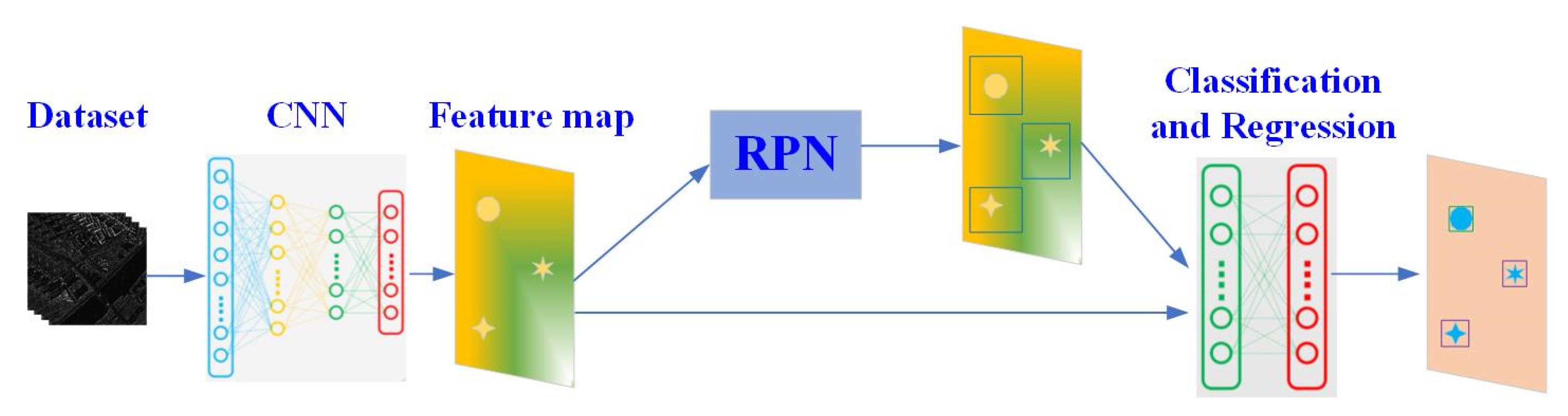
Faster R-CNN has been presented to solve the problem that fast R-CNN framework spends most of its time on the Selective Search extraction box instead of classification. In faster R-CNN, it replaces the search selective algorithm of the fast R-CNN network with RPN, saving plenty of time. Moreover, RPN, classification and regression share the same feature extraction network, which improves the speed of the model. The overall architecture of faster R-CNN is shown as Figure 1. The dataset is first inputted into the CNN to extract feature maps, and then proposed regions are obtained through RPN. Moreover, the proposed regions and the previously obtained feature maps are used to classify and regress the targets to generate precise positions of each type of targets.

In the RPN, after the feature map is extracted by the convolutional layer, the RPN will slide an n × n window on the feature map (default n = 3) and generate k region proposals according to a certain ratio and aspect ratio at each window position. By default, there are three ratios and three aspect ratios, so nine region proposals are generated. Then it goes through two 1 × 1 convolution layers, one layer is used for classifications, determining whether each region proposal contains the target to be detected, and outputs 2 × k scores. The other layer is used for proposals regression, and outputs 4 × k coordinates correspond to k region proposals.

3.2. The Framework Architecture

The architecture of the proposed framework is shown in Figure 2, namely multi-resolution attention and balance network (MABN), which is based on the framework of faster R-CNN. In this paper, we use the proposed attention and balanced feature pyramid (ABFP) network to generate feature maps instead of CNN in faster R-CNN. In which, the balanced feature pyramid (BFP) [10] and the attention mechanism [11] are incurred to further extract the essential features. Because the BFP can aggregate low-level and high-level features better simultaneously. While the attention mechanism can focus more on the useful information of the target and suppress the useless information. Therefore, we introduce them to achieve bridges detection with high precision.

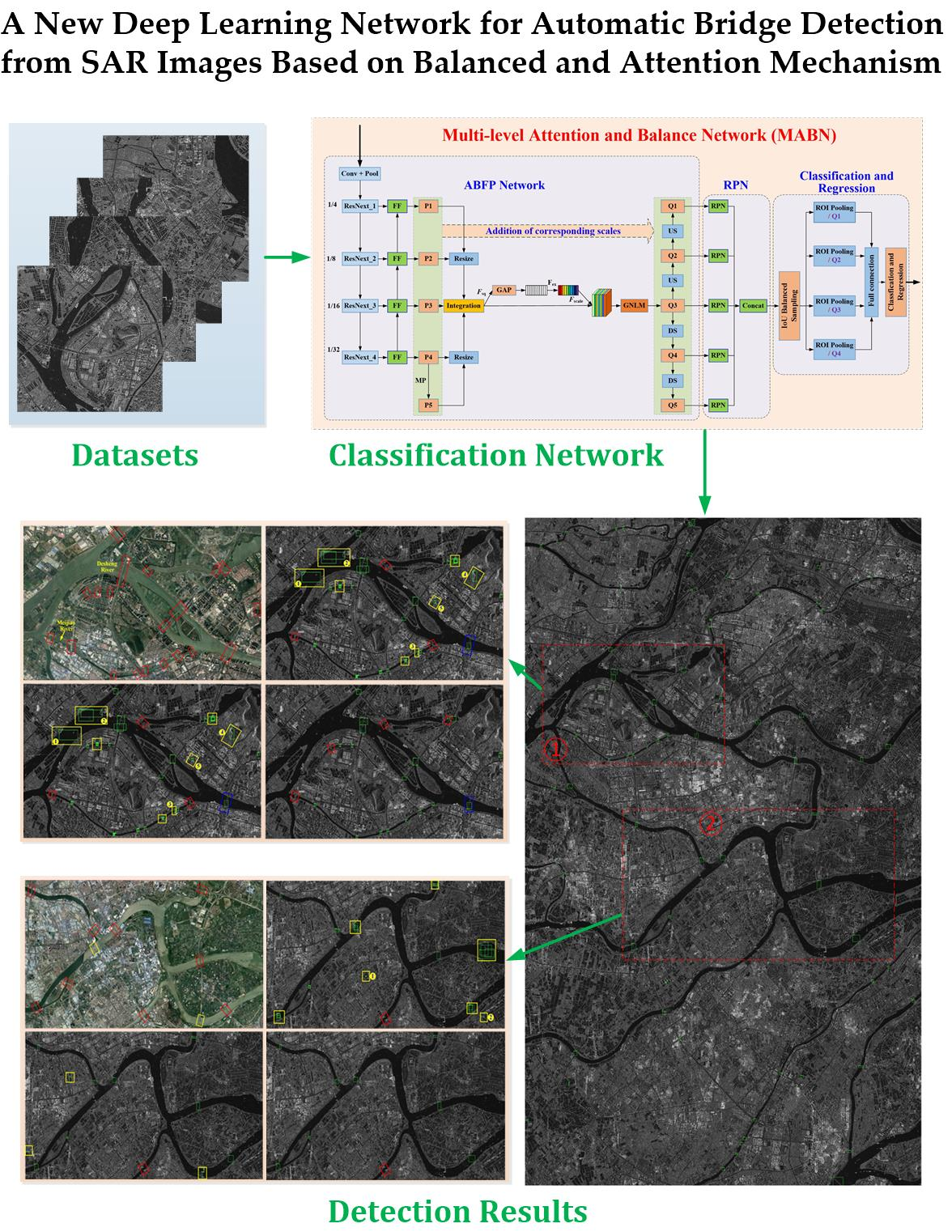
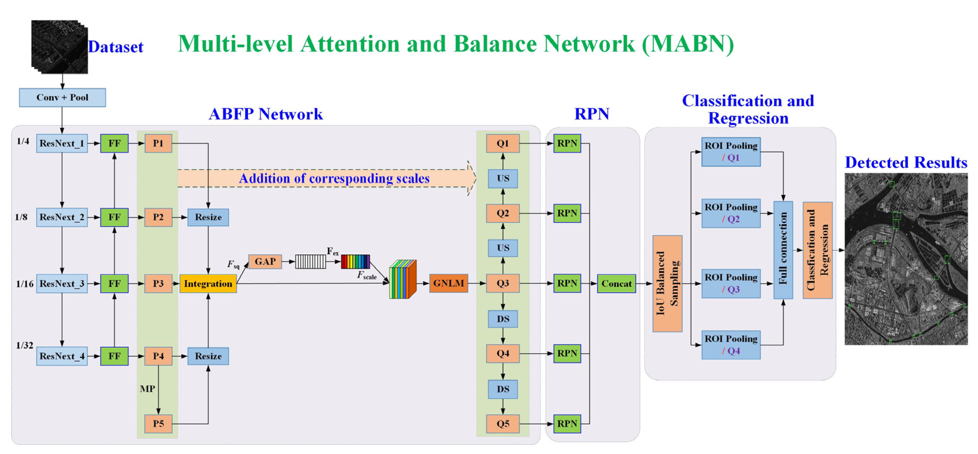
MABN mainly contains three parts, namely, ABFP network, RPN, and classification and regression. First, the produced bridge dataset is inputted to the backbone network—ResNeXt [9], which mainly consists of four residual blocks, namely, ResNeXt_1, ResNeXt_2, ResNeXt_3, and ResNeXt_4. The feature map generated by each convolution module is then input to features fusion (FF) module to achieve features fusion from different resolutions. Thus, we obtain feature maps at 4 scales, P1, P2, P3, and P4. To obtain more advanced features, we use maximum pooling on P4 to produce the feature map P5. Then, these feature maps are transformed to the scale of P3 by ‘Resize’ operation and fused together. After that, the fused feature map is weighted by the attention mechanism and enhanced by the Gaussian non-local module (GNLM) [31] to produce the feature map Q3. To utilize the features with different resolutions while generating the candidate boxes, the feature maps of the same scale as P1 to P5 are obtained by up-sampling and down-sampling respectively on Q3, then we get Q1, Q2, Q4, and Q5. Moreover, the feature maps of corresponding scales (P1–P5) are added to the feature maps Q1–Q5, and then they are inputted to the RPN to extract the candidate boxes of the targets.

In the RPN module, For the feature map at each scale, predicted bounding boxes are generated. Then, a fixed-length feature vector is obtained through ROI Pooling, and input into the fully connected layer. Finally, classification and regression are performed to obtain detected results of the objects. During the training of classification and regression module, IOU balanced sampling and balanced L1 loss function are introduced to better utilize the hard samples and control simple samples.

3.3. ABFP Network

The proposed ABFP network mainly employs ideas of the balanced feature pyramid and the attention mechanism. The balanced feature pyramid can sufficiently utilize the features of different resolutions, and the attention mechanism can adequately make use of the features by weighting the features according to their importance for targets detection.

3.3.1. ResNeXt

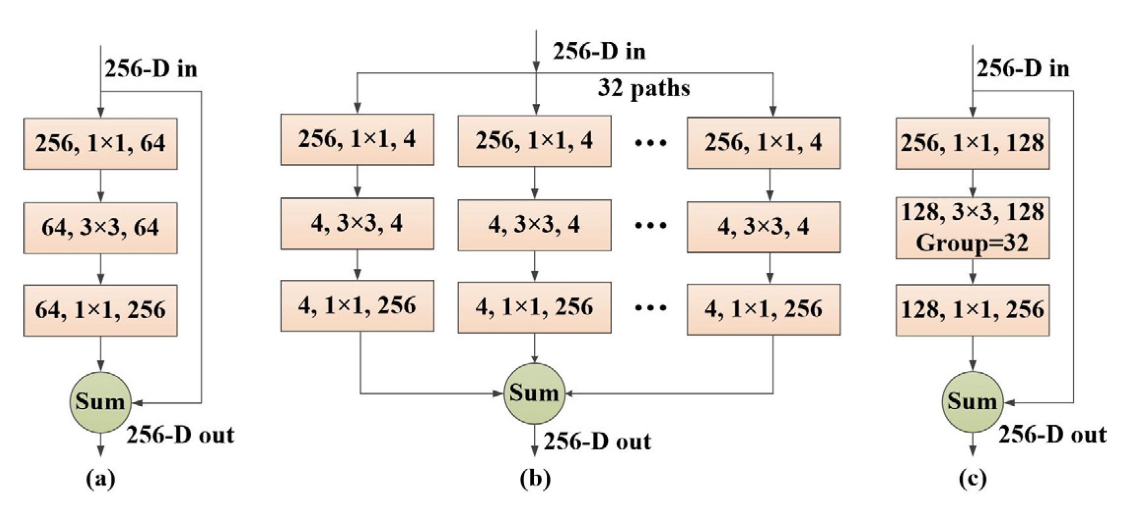
ResNeXt [9] is the latest upgrade of the ResNet [32], and its basic structure has changed a lot. In Figure 3a,b, basic structures of the two networks (ResNet and ResNeXt) are given. It can be found that in ResNeXt, the basic structure has become the same branch of the 32-channel topology. For further simplification, it has a structure similar to Inception if concatenating the outputted 1 × 1 convolutions together, and then combining the inputted 1 × 1 convolutions to get the result shown in Figure 3c, which uses grouped convolutions. The group parameter is used to limit the convolution kernel of this layer and the convolution of the input channels, which can reduce the amount of calculation. Here, 32 groups are used, and the input and output channels of each group are 4, and the channels are finally merged. Figure 3c is more concise and faster, so this structure is generally used. The core innovation of ResNeXt is to replace the three-layer convolutional blocks of the original ResNet with a parallel stack of blocks of the same topology, which greatly improves the accuracy of the model without significantly increasing the magnitude of the parameters. Hyperparameters are also reduced to facilitate model migration.

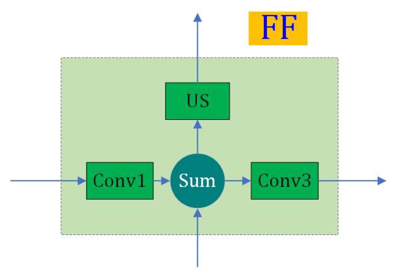
Figure 4 indicates the Feature Fusion (FF) module. First, it convolves the features generated by ResNeXt block of the same resolution channel, which is added with the features from lower resolution channel. Then, the sum is used by two aspects. On one hand, it is up-sampled (US) to a higher resolution channel. On the other hand, it is convolved to output the features. For the highest resolution channel, there is no up-sampling operation.

3.3.2. Balanced Feature Pyramid

High-level features extracted through convolutional neural networks pay more attention to semantic information, while low-level features more reflect detailed information. The feature pyramid network (FPN) [33] improves the target detection performance by integrating the features of different layers through horizontal connections, which integrates the information of adjacent resolutions. If the integrated features contain information of all resolutions, it is more conducive to target detection. The balanced feature pyramid network (BFPN) [10] is used to enhance the original features by integrating the balanced features obtained from all resolutions with the same information, thus, the extracted features are more discriminative.

First, all feature layers of different resolutions are scaled to the same resolution, and then a simple weighted average is performed to produce a balanced feature layer (shown in Figure 2).

$$\tilde{C}=\frac{1}{L}{\displaystyle \sum }_{i=l}^L{C}_i$$

(1)

where $L$ is the number of the layer.

Finally, the obtained features are rescaled to different resolutions to enhance the original features, so that each resolution has the same information obtained from other resolutions. Then the original features of different resolutions are added to the corresponding final features. Finally, the feature balance is achieved.

3.3.3. The Introduction of the Attention Mechanism

•Attention mechanism

When the human brain is active, it will automatically focus on the areas of interest and ignore the areas that are not of interest. This is an embodiment of the human brain’s attention mechanism. The attention mechanism in deep learning is essentially similar to the attention mechanism of the human brain, and the purpose is to obtain information that is more effective for the current task among considerable information. At present, the attention mechanism is widely used in the field of image segmentation and object detection.

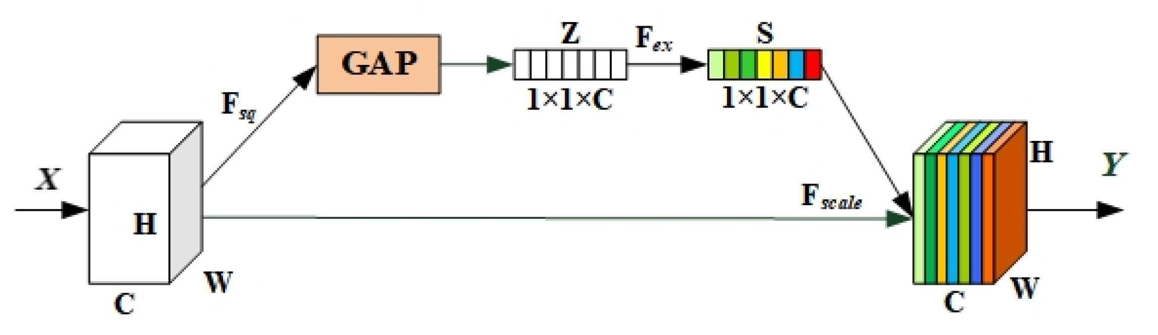
In this paper, the squeeze and-excitation (SE) [11] block is used to model the interdependent relationship between image channels. Each feature channel has a degree of importance, and a weight is automatically obtained through learning. This weight is used to enhance useful features and suppress those useless features. The importance of feature channels and the corresponding weights obtained are the embodiment of the attention mechanism. The basic structure of SE block is shown in Figure 5.

As shown in Figure 5, X is input into the main branch of the SE block, and a convolution operation is performed to generate a feature map with the size of W × H and the channel number of C. Then, the global average pooling (GAP) is used to accomplish the “squeezing” process. The number of feature channels does not change, and a feature map with the size of 1 × 1 × C is generated. Currently, the feature map has a global receptive field.

$${\overline{X}}_C=F_{Sq}\left(A_C\right)=\frac{1}{W\times H}{\displaystyle \sum }_{i=1}^H{\displaystyle \sum }_{j=1}^W{\alpha }_{ij}$$

(2)

where $A_C$ and ${\overline{X}}_C$ denote the feature maps before and after pooling, and ${\alpha }_{ij}$ stands for any pixel in $A_C$.

A “bottleneck” structure is formed by two fully connected (FC) layers to fit the correlation between feature channels. After performing two FC transformations on the feature map with the size of 1 × 1 × C, a weight vector with the dimension of C is obtained, and then the vector is normalized to 0 to 1 by the Sigmoid activation function sig.

$$Z_C= F_{ex}\left({\overline{X}}_C\right)=sig\left(\delta \left({\overline{X}}_C\right)\right)$$

(3)

where $Z_C$ represents the obtained weight vector, and $\delta$ denotes the “bottleneck” structure.

Then, the obtained weight vector is weighted to the original feature channel by the scale operation.

$${\tilde{X}}_C= F_{Scale}\left(Z_C,A_C\right)=Z_C·A_C$$

(4)

The importance of each feature channel in the feature map is calculated by the SE block, and a weight vector is obtained, which is then weighted to the original feature map. This stimulates effective features, suppresses redundant features, and implements a feature recalibration process.

•The introduction strategy

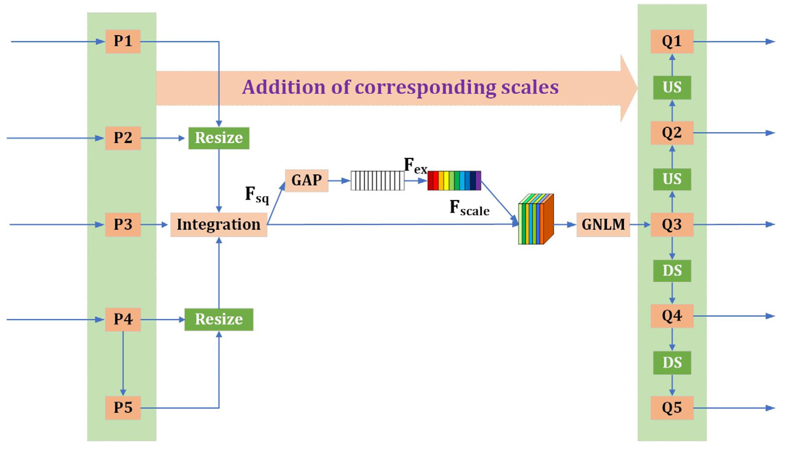
In order to make the acquired features more discriminative and improve the accuracy of the model, this paper skillfully combines the attention mechanism with the balanced feature pyramid. The specific structure is shown in Figure 6. For the feature maps at 5 scales (P1, P2, P3, P4, and P5) generated by the ResNeXt network and the balanced feature pyramid, resize the feature maps of the other 4 scales to the P3 scale and integrate them to obtain a unified scale feature map with different resolution features. Furthermore, the attention mechanism is applied to the feature map to obtain weights, and the rescaling of the feature map is achieved to generate a new feature map Q3. Moreover, Gaussian non-local modules (GNLM) [1] are used to enhance the features, and then up-sampling and down-sampling operations are used to obtain feature maps Q1 to Q5 on the same scale as P1 to P5. After that, for fully utilizing the features, the feature maps of the corresponding scales of P1–P5 and Q1–Q5 are added and input to the next network structure for further processing. The features of the feature map obtained after weighting and multiple enhancements are more obvious and more representative, and the detection effect of the model will be better.

3.4. Region Proposal Network

Region proposal network (RPN) can be understood as a kind of full convolutional network, which can perform end-to-end training with the purpose of giving candidate boxes. RPN slides an n × n window (n = 3 by default) on the feature map, and generates k anchors at a certain ratio and aspect ratio at each window position. The default is three ratios and three aspect ratios. Thus, nine anchors are generated. After that, it goes through two convolutional layers (each is 1 × 1 convolution). One layer is used for classifications of two types. It determines the probability of each anchor as the target to be detected, and outputs 2 × k scores. Another layer is used for anchor regression, and 4 × k coordinates correspond to k anchors are outputted. If the size of the feature map is W × H, then W × H × k anchors are generated.

Due to the large number of anchors, RPN will select some positive samples and negative samples for training. If the IOU value of the anchor box and the ground-truth box is the largest or greater than 0.7, it is a positive sample; if the IOU value is less than 0.3, it is a negative sample; if it is neither positive nor negative sample, it will not be involved in training. The loss function defined during training is as follows, which can be used to optimize the classification and regression of prediction bounding boxes.

$$L\left(\left\{p_i\right\},\left\{t_i\right\}\right)=\frac{1}{N_{cls}}{\displaystyle \sum }_i{L}_{cls}\left(p_i,p_i^{\ast }\right)+\lambda \frac{1}{N_{reg}}{\displaystyle \sum }_i{L}_{reg}\left(t_i,t_i^{\ast }\right)$$

(5)

where $L_{cls}$ and $L_{reg}$ are classification loss and regression loss respectively. $i$ is the subscript of anchors. $p_i$ represents the predicted probability that the i-th anchor, $p_i^{\ast }$ is a value according to the sample type, if the i-th anchor is a positive sample, $p_i^{\ast }=1$; else, $p_i^{\ast }=0$. $t_i$ and $t_i^{\ast }$ denote the coordinates of the predicted bounding box and the ground-truth box respectively. $N_{cls}$ and $N_{reg}$ are the mini-batch size and the number of anchor locations, and $\lambda$ is used to balance the weight of the loss.

3.5. Classification and Regression

First, the network generates candidate boxes on the feature maps through RPN, and then these candidate boxes from different scales are sent to the ROI pooling module [8] and mapped onto the feature maps with the corresponding scales. Moreover, a fixed-length feature vector is generated and a performed is then max pooling operation. Furthermore, perform a full-connect operation on this feature vector, use the Softmax layer to classify specific categories, and obtain the precise location of objects by regression. After the classification of each region is completed and the corresponding confidence level is obtained, the non-maximum value suppression (NMS) [34] is used to remove the overlapping boxes to generate the final target region.

3.5.1. IoU Balanced Samples

Faster R-CNN uses step-by-step training. First, pre-trained model is used to initialize the network and train the RPN by end-to-end. Then candidate boxes generated by PRN are utilized to train fast R-CNN, and finally they are combined for fine-tuning training. In fast R-CNN training, the stochastic gradient descent (SGD) [35] is employed to train the network and update related parameters. SGD mini-batch is randomly selected in the training set, and each mini-batch contains N images and B samples, that is B/N samples per image. If the intersection over union (IOU) values of these samples and ground-truth box are greater than 0.5, they are positive samples; and if the values between 0 and 0.5, they are negative samples. The negative samples that are easily identified as positive samples are difficult negative samples, which can be trained to improve the classification and regression performance of the network. This shows [10] that the overlap area of more than 60% of the difficult negative samples with their corresponding ground-truth box is greater than 0.05, and only 30% of such samples are selected by random sampling in the mini-batch, which makes the network training unbalanced. To solve this problem, we have introduced IOU balanced sampling [10].

In random sampling, the probability that each sample is selected is

$$P= N/M$$

(6)

where N represents the number of negative samples we need to select, and M indicates the corresponding candidate boxes.

Because the sampling is random, so the selected samples are not uniform. To overcome this difficulty, the IOU balanced sampling divides the sampling interval into K intervals evenly according to values of the IOU, and N negative samples are evenly distributed to each interval. This ensures the uniformity of the samples, i.e., balanced sampling is achieved. The formula is as follows.

$$P_K=\frac{N}{K}·\frac{1}{M_K}$$

(7)

where $M_K$ represents the number of candidate boxes of the corresponding interval, and the default value of $K$ is 3.

3.5.2. Loss Function

Each region proposal used for training has a real category label and an accurate bounding box. In this paper, the multi-task loss function is used to jointly optimize the classification and the bounding box for training, which is defined as

$$L_{p,u,t^u,v}= L_{cls}\left(p,u\right)+\lambda \left[u\ge 1\right]L_{loc}\left(t^u,v\right)$$

(8)

where $L_{cls}$ and $L_{loc}$ represent loss functions of classification and positioning respectively, and $t^u$ denotes the regression result of category $u$. $p$ and $u$ stands for the predicted box and the ground-truth box. $v$ is the targets of regression, and $\lambda$ is used to adjust the weight of the loss.

Usually, $\lambda$ is adjusted directly to balance the classification and positioning of the two objective functions. This will unbalance the sample gradients and affect the training effect of the model. Therefore, a balanced L1 loss function is introduced. Inspired by smooth L1 loss [24], the positioning loss function is defined as follows:

$$L_{loc}= {{\displaystyle \sum }}_{i\in \left\{x,y,w,h\right\}}{L}_b\left(t^u-v_i\right)$$

(9)

where $L_b$ is the balanced L1 loss function.

The following formula is defined according to the gradient relationship.

$$L_b\left(x\right)= \{\begin{array}{l}\frac{\alpha }{b}\left(b\left|x\right|+1\right)\ln \left(b\left|x\right|+1\right)-\alpha \left|x\right| if \left|x\right|<1\\ \gamma \left|x\right|+C otherwise\end{array}$$

(10)

where $\alpha$ is used to control the gradient of simple samples (Samples with small gradients). The smaller the $\alpha$ is, the larger the gradient is. $\gamma$ is utilized to adjust the upper limit of the regression error to help the objective function better balanced related tasks. $b$ is used to ensure that the values of the above formula are the same at $x=1$.

The relation of $\gamma$, $\alpha$ and $b$ is

$$\alpha ·ln\left(b+1\right)=\gamma$$

(11)

Parameters are set to $\alpha =0.5$ and $\gamma =1.5$.

3.5.3. The Strategy of Reducing False Alarm

In this paper, non-maximum suppression (NMS) [34] is used to reduce false alarms, which is a process of searching local maximums. In the process of target detection, multiple candidate boxes are usually generated at the same target position, and they overlap each other. Therefore, we need to remove the redundant candidate boxes and keep the box that best matches the target position. After the network generates candidate boxes, it will calculate a confidence level for each one. We arrange the confidence levels from high to low, select the box with the highest confidence level, calculate the degree of overlap between it and other boxes, and delete the box whose IOU is greater than the threshold. The threshold can be set independently, which is usually 0.5. The box with the highest degree of confidence is selected to indicate that it is the box that we have preserved. Then, select the box with the highest confidence among the remaining candidate boxes and repeat the above operation. After repeating the operation several times, the candidate box that best matches the target is achieved.

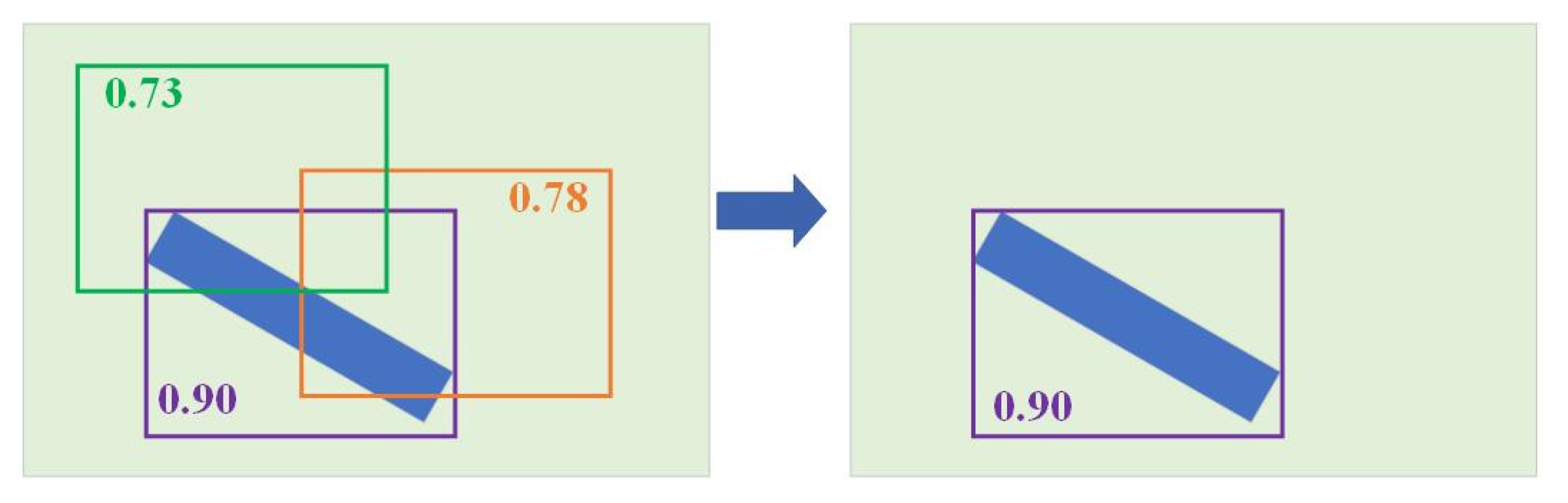
The simple sketch map of NMS is shown in Figure 7. In which, three candidate boxes have been generated for one target, and a confidence levels for them are 0.73 (green box), 0.78 (orange box), and 0.90 (purple box) respectively. After the NMS operation, the candidate boxes with low confidence and overlap greater than the given IOU threshold will be removed, leaving the candidate box with a confidence of 0.9. The bridges to be detected in this paper are slender targets, and the overlap between targets is small. Therefore, the IOU threshold value selected in this paper is 0.1, that is, the candidate boxes with low confidence and overlap greater than 0.1 will be removed.

3.6. The Implementation of Training

The process of training for the proposed bridge detection network is as follows.

In this paper, the proposed bridges detection network, MABN, is still trained step by step like faster R-CNN, using the ImageNet pre-trained model to initialize the network parameters. The details are as follows:   Input: SAR datasets, containing all SAR images with the size of 500 × 500, and the corresponding labels.   1: Utilize the pre-trained model to initialize the network and train the RPN by end-to-end.   •Extract multi-resolution feature maps using ABFP network.   •Perform end-to-end training of RPN through back propagation (BP) algorithm and stochastic gradient descent (SGD), calculate loss function, and generate candidate boxes.   •Loss function: $$L\left(\left\{p_i\right\},\left\{t_i\right\}\right)=\frac{1}{N_{cls}}{\displaystyle \sum }_i{L}_{cls}\left(p_i,p_i^{\ast }\right)+\lambda \frac{1}{N_{reg}}{\displaystyle \sum }_i{p}_i^{\ast }{L}_{reg}\left(t_i,t_i^{\ast }\right)$$ where $L_{cls}$ and $L_{reg}$ are classification loss and regression loss respectively. $i$ is the subscript of anchors. $P_i$ represents the predicted probability of the i-th anchor, and $p_i^{\ast }$ is a value according to the sample type, if the i-th anchor is a positive sample, $p_i^{\ast }=1$; else, $p_i^{\ast }=0$. $t_i$ and $t_i^{\ast }$ denote the coordinates of the predicted bounding box and the ground-truth box respectively. $N_{cls}$ and $N_{reg}$ are the mini-batch size and the number of anchor locations, and $\mathsf{\lambda }$ is used to balance the weight of the loss.   2: Use the candidate box generated by PRN to train fast R-CNN.   •Extract multi-resolution feature maps using ABFP network.   •Map the candidate boxes to the multi-resolution feature map and obtain a fixed-length feature vector by the ROI Pooling layer.   •Perform a full-connect operation on the fixed-length feature vector and put it into the classification and regression layers, calculate a multi-task loss function to optimize network parameters, and obtain a network model.   Loss function: $$L_{p,u,t^u,v}=L_{cls}\left(p,u\right)+\lambda \left[u\ge 1\right]L_{loc}\left(t^u,v\right)$$ where $L_{cls}$ and $L_{loc}$ represent loss functions of classification and positioning respectively, and $t^u$ denotes the regression result of category $u$. $p$ and $u$ stand for the predicted box and the ground-truth box respectively. $v$ is the targets of regression, and $\lambda$ is used to adjust the weight of the loss.   3: The weight of the ABFP network is generated, and the steps of RPN training are simulated to fine-tune the unique layers of RPN.   4: Ensure that parameters of the ABFP network and RPN weight are unchanged, and use the candidate boxes output from the previous step to imitate the training steps of fast R-CNN to adjust its unique layer.   Output: The trained model by the proposed network for bridges detection.

4. Experiments and Results

4.1. The Data Used in this Paper

In this paper, the data used in the experiments are 3-m resolution SAR images obtained by TerraSAR system and 1m-resolution SAR images from Gaofen-3 system. We also note they have been calibrated already. There are two large-scale scene images with sizes of 28,887 × 15,598 and 30,623 × 14,804, which are acquired from the Dongtinghu and Foshan areas of China, respectively. In addition, there are several large-scale Gaofen-3 SAR images are utilized. We use PhotoShop tools to crop 1560 bridge slices with size of 500 × 500 on two SAR images as samples, and use the LabelImg tool to label the bridges in the sample, which are divided into two categories: background and bridge. In this experiment, only bridges over water are labelled. Further, 80% of the pictures are selected as training samples and 20% of the pictures are used as verification samples. 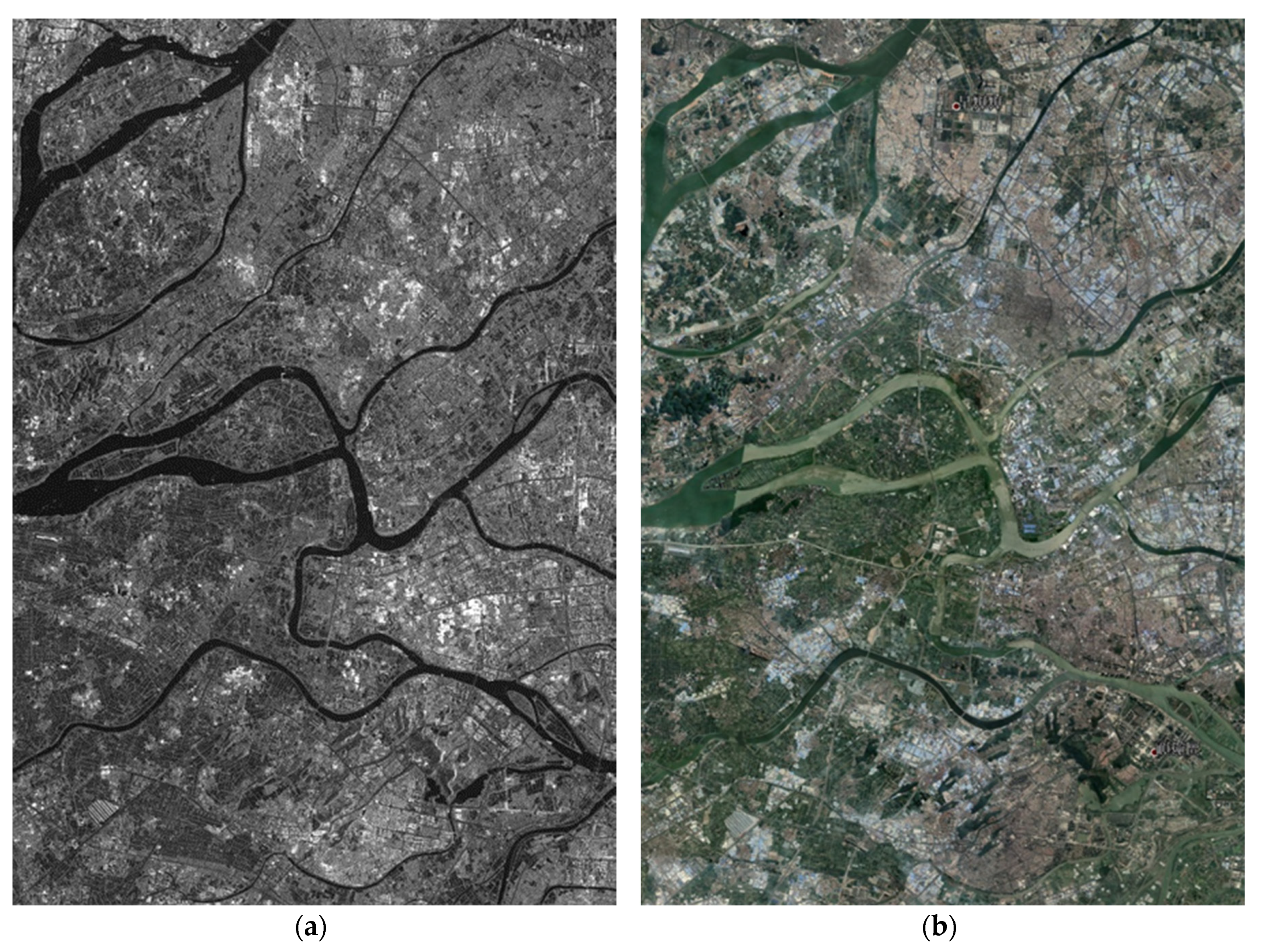Figure 8 shows a part of SAR image and corresponding optical image of Foshan city. Here, we can see that there are many bridge targets.

4.2. Results and Analysis

To evaluate the effectiveness of the proposed network in this paper, we compared the detected results of bridges by the proposed algorithm with faster R-CNN and SSD. In this experiment, three indicators [36] are utilized to assess the detection performance of the network, namely, recall rate (RR), precision (P), and average accuracy (AP). RR represents the probability of each category being detected correctly; P denotes the probability of detected targets being correctly classified; AP is used to measure the overall performance of the network, which is the area of P (vertical axis) and RR (horizontal axis). Generally speaking, the classification performance is better if the AP value is higher. However, many false alarms can’t be reflected in RR and AP, so P is necessary. The equations of them are shown as follows.

$$RR=\frac{TP}{TP+FN}$$

(12)

$$P=\frac{TP}{TP+FP}$$

(13)

where $TP$ denotes the number of targets correctly detected as category A, and $FP$ is the number of false detections as class A. While $FN$ indicates the number of missing targets for category A.

The evaluation index of each network is shown in

Table 1. The performance of bridges detection by different networks.

Network	RR	P	AP
Faster-RCNN	0.920	0.100	0.750
SSD	0.971	0.322	0.894
Ours	0.917	0.877	0.896

. As we can see from the comparison of the data in the table, faster R-CNN has the lowest precision and AP, especially P is very low (only 0.1) though RR is high (0.92). It indicates that there are a large number of false alarms though many targets are detected, so the overall network performance for bridges detection is poor. SSD acquires the highest value in RR and higher value in AP and P than faster R-CNN, which denotes the overall performance has been improved compared to faster R-CNN. However, its P is still low (just 0.322), that’s because it still doesn’t solve the problem of many false alarms. The AP obtained by the proposed network is not much higher than SSD, and even the RR is slightly lower than SSD, but its precision has been improved by 1.8 times than SSD. It indicates that the network proposed in this paper greatly reduces the false detection and false alarms that occurred in the previous two networks, and greatly improves the performance for bridge detection from SAR images.

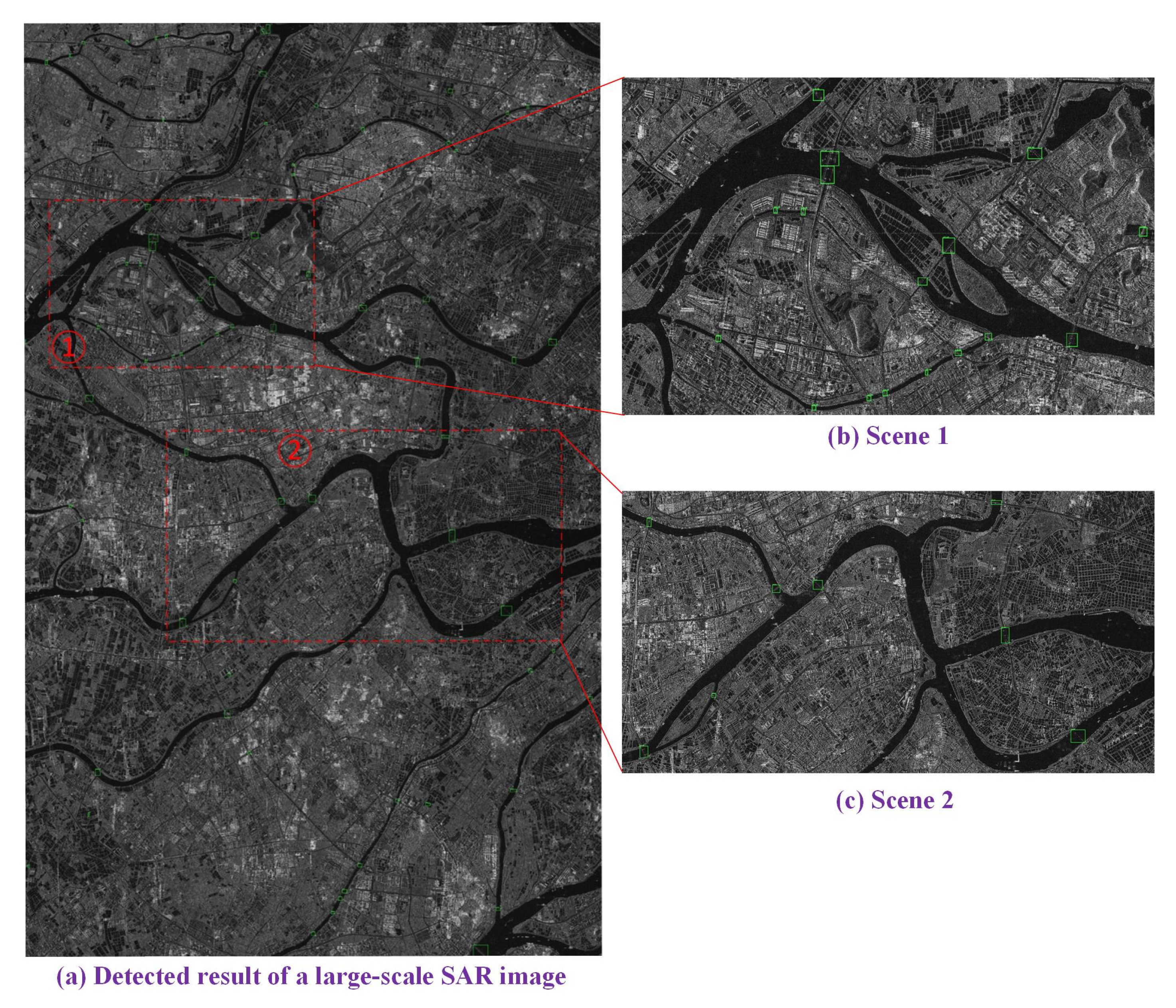
In this experiment, a part of TerraSAR image (Foshan City) with size of 17,000 × 10,500 and a SAR image from Gaofen-3 system are utilized to test the performance of the proposed network, which are not used in training and verification. Figure 9a shows the detected results of bridges by the proposed network for this part of SAR image from TerraSAR system. This indicates that all the bridges have been nearly detected, which are shown in the green boxes. There is a total of 75 bridges with different sizes in this large-scale image. Using the proposed network, 74 targets have been detected, of which 69 are bridges and 5 are non-bridge targets. Therefore, the RR and the P for bridges in this test are 92% and 93.24% respectively, and the false alarm rate is 6.76%. From which, we can see the proposed network can implement bridges detection with much high precision, and there are few false alarms and missed bridge targets. For further comparison of the detected results, two scenes with more concentrated bridges in Figure 9a are analyzed separately in detail (the two red boxes, which are correspondingly illustrated in Figure 9b,c).

4.2.1. Analysis of Bridges Detection in Scene 1 for TerraSAR Image

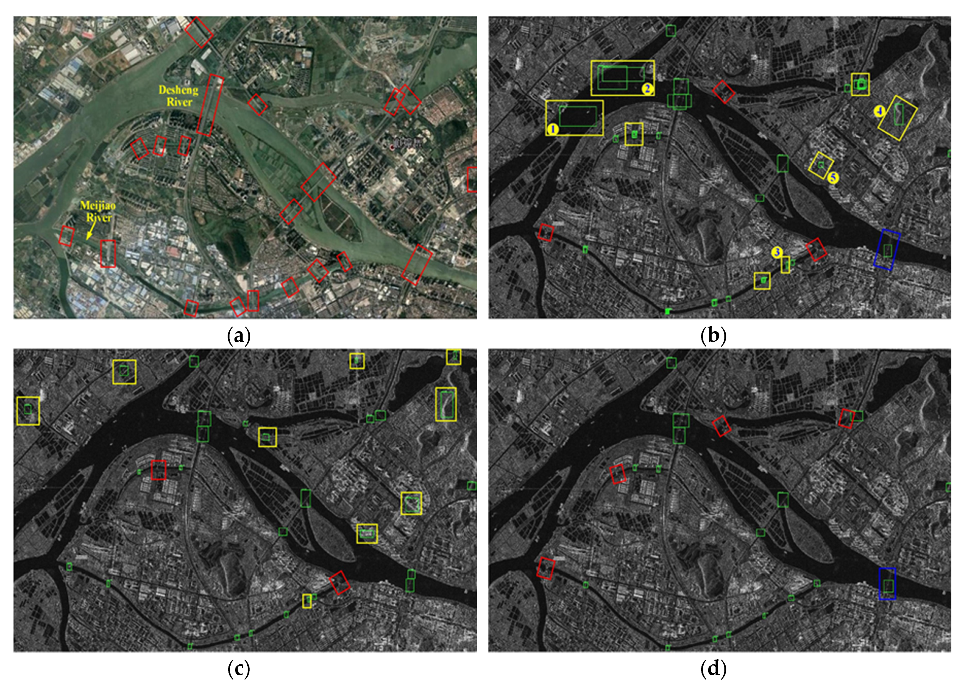
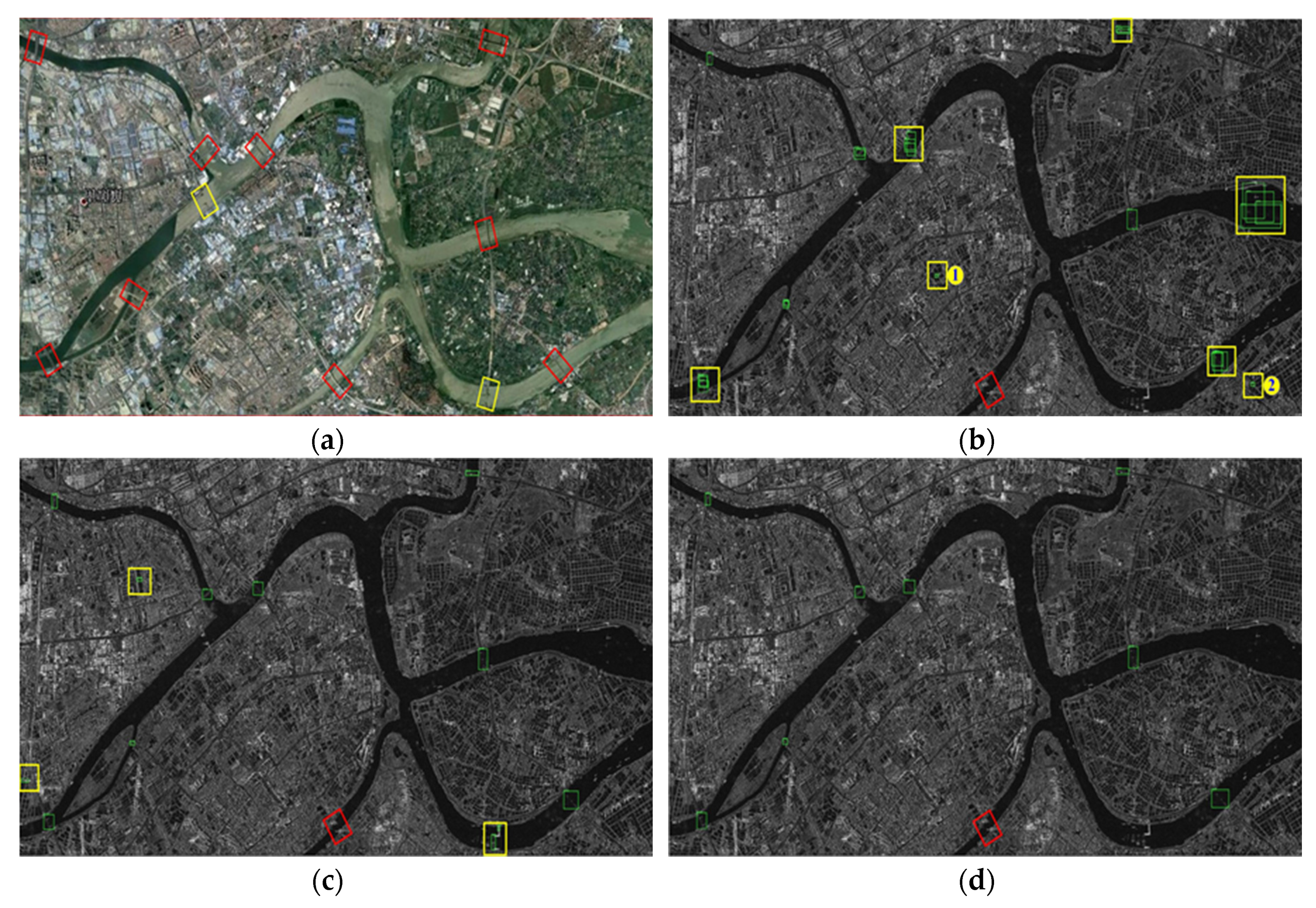
Figure 10 depicts the corresponding optical image and detected results of bridges from SAR images for Scene 1, which is a small area in Shunde District. According to Figure 10a, there are 20 bridge targets of different widths and lengths in total, which are marked by red rectangles. Several large-scale bridges are all located over the Desheng River, and there are 8 bridges over Meijiao River.

Figure 10b shows the detected results of bridges by faster R-CNN. From which we can see most of the bridges have been detected, which are given with green boxes. However, there are also many false alarms, which are marked by yellow rectangles. There are mainly three types of false alarms. The first case is the non-bridge targets on the water are detected as bridges, such as ships (the areas marked by yellow rectangles with 1 and 2) and bridge-like linear targets (the yellow rectangle labeled 3). The second case is that targets similar as bridges on land are mis-detected as bridges, such as the yellow rectangles labeled 4 and 5. The area labeled 4 is actually a ridge, maybe the amplitude of the image on its both sides is lower, so it is detected as a bridge. The third case is that a bridge is repeatedly detected by multiple boxes, such as the several other typical areas marked by yellow boxes. In addition to false alarms, there are several undetected bridges, such as three bridges marked by red rectangles. Furthermore, there is a bridge which is detected incompletely (marked by a blue rectangle). From the above analysis, it can be known that faster R-CNN network cannot distinguish the characteristics of different targets well from SAR images, which results in a weak capability for bridge detection.

Figure 10c illustrates the bridges detection results by SSD. According to the result, we find nearly all the bridges are detected except two small bridges (marked by red rectangles). However, there are still many false alarms (marked by yellow rectangles), which are very different from the false alarms in the detected results generated by faster R-CNN. There is basically only one false alarm situation, that is, similar targets on land are detected as bridges, and there are no repeated detection and basically no false detections of targets on the water as bridges. In addition, there are no cases of detecting bridges incompletely.

Figure 10d demonstrates the detected result of bridges by the proposed network in this paper. We find there is no false alarm in the result, but there is two more undetected bridges than SSD, and an incomplete detected result also appears.

4.2.2. Analysis of Bridges Detection in Scene 2 for TerraSAR Image

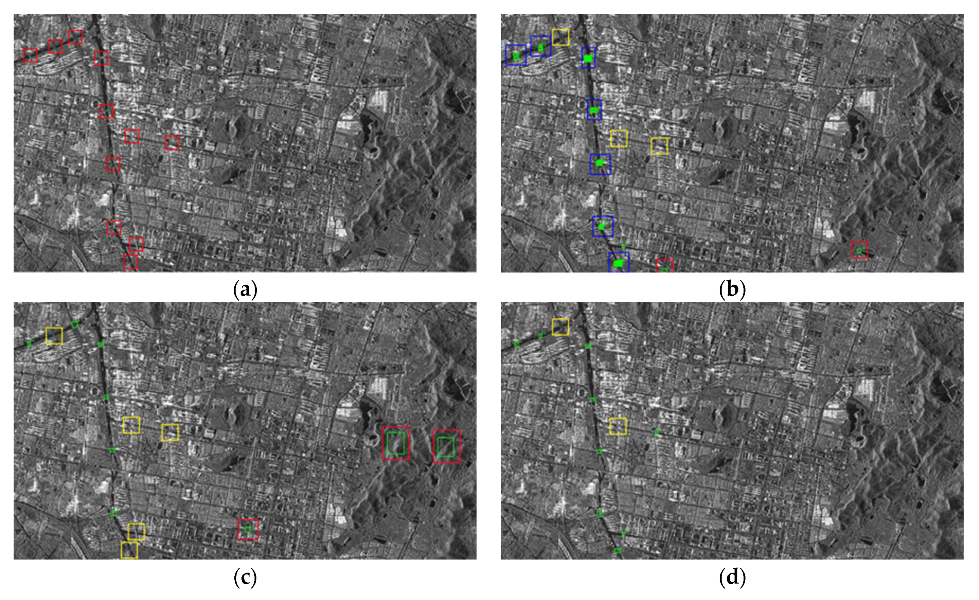
Figure 11 shows the corresponding optical image and detected bridges by faster R-CNN, SSD and the proposed network in this paper. Figure 11a is the optical image, in which we can see there are nine obvious large bridges, which are marked by red rectangles. For the two bridges marked by yellow rectangles, since they have been severely disconnected in the middle section, no detection is performed in this paper.

Figure 11b is the detected result for bridges by faster R-CNN network. It can be seen that there are many false alarms in several yellow marked boxes, mainly the case where there are multiple repeated detection boxes for one target except the boxes labeled 1 and 2, which are detected as bridges, but are actually the edges of the ponds. We find there is an undetected bridge which is marked by a red rectangle. Although this bridge is very obvious in the optical image, it breaks a larger piece in the middle in the SAR image, so it is difficult to detect. Figure 11c illustrates the result generated by SSD. There are three false alarms (marked by yellow boxes) appearing in this result, of which two are edges of the pond, and the other one is the broken bridge. It also has not detected the bridge undetected by faster R-CNN. Figure 11d demonstrates the detected result of bridges by the proposed network in this paper. As can be seen from the figure, the network has detected all the bridges (except that broken bridge marked by red box), and there is no false alarm. Therefore, the proposed network in this paper can perform bridges detection very well.

4.2.3. Analysis of Bridges Detection for Gaofen-3 Image

Figure 12 indicates the detection results of bridges for Gaofen-3 SAR image. Figure 12a is the ground truth of the bridges, in which the bridges are marked by red boxes. From which we can see the background of the bridges is complex, and the bridges are not long. Figure 12b shows the result of bridges generated by faster R-CNN. As shown in Figure 12b, there are three missed bridges (marked by yellow boxes), two false detections (marked by red boxes), and many overlapping boxes for multiple detections (marked by blue boxes). Figure 12c illustrates the detection results of SSD, in which there are three false detections (marked by red boxes) and five missed bridges (marked yellow boxes), but no multiple detections. Figure 12d gives the detections by MABN. We find that there are only two missed bridges (marked by yellow boxes), but there are no false detections and multiple detections.

Through the analysis of the extracted bridge results of the above three scenarios, it can be known that both Faster R-CNN and SSD are prone to generate many false alarms, in which the same bridge has multiple detection boxes and similar targets are detected as bridges. While the network proposed in this paper (MABN) is basically free of false alarms. In addition, there are all missed detection for three networks, but MABN has the least. Furthermore, both faster R-CNN and MABN have incomplete bridge detection (in the first and second scenes), which does not occur in the SSD networks. Based on the above analysis, it is known that for bridges detection, the proposed network in this paper (MABN) has the best bridge detection performance, and the advantages are much obvious.

5. Discussion

In the paper, we propose a new deep learning network, MABN, which obtains the best performance for bridges detection from SAR images, compared with Faster R-CNN and SSD. Because we incur attention mechanism, which can extrac useful information about targets to be detected, and suppress irrelevant information. In addition, we introduce the Balanced Feature Pyramid (BFP), IOU balanced sampling, and improved L1 Loss function. BFP utilizes the integrated balanced semantic features with the same depth to enhance multi-level features. IOU balanced sampling greatly improves the selection probability of hard negative samples, thereby effectively enhances the detection performance. The improved L1 Loss function promotes crucial gradients and balances the involved classification and accurate localization. All these incurred strategies highly increase the precision of bridges detection.

However, we also note there are still missed detections in MABN, although it has few false alarms and no multiple detections. This indicates the performance of bridge detection should be improved further to reduce the missed detection rate, which will be considered in our following research. In addition, bridge detection from SAR images with different bands and different resolutions will also play a pivotal role in our further research with the utilization of transfer learning.

6. Conclusions

To accomplish end-to-end bridge detection with high precision from SAR images, a new deep learning network, MABN, is proposed. The network integrates ResNeXt, balanced feature pyramid, RPN and attention mechanism. It mainly contains three parts, namely, the proposed ABFP network, RPN, and the classification and regression module. The ABFP network includes the ResNeXt, and the fused structure of balanced feature pyramid (BFP) and attention mechanism (AM). In this part, feature maps with different resolutions are generated by the ResNeXt at first, and then they are inputted into the fused structure to further extract the essential features with different levels, in which the information from different resolutions and different channels are handled. Moreover, these more distinctive features are processed by the RPN to produce candidate boxes at different levels for bridges. After that, classification and regression are performed on these candidate boxes to generate final detected results for bridges, in which, NMS are employed to enhance the detection precision. Furthermore, IOU balanced sampling and balanced L1 loss functions are introduced for balancing the training of classification and regression network.

Compared with faster R-CNN and SSD in the experiment with TerraSAR and Gaofen-3 images, the proposed network in this paper presents much better performance in bridges detection with complex background. It can reach 0.877 in P and 0.896 in AP, which are the highest of the three networks. The precision in P for Faster R-CNN and SSD are only 0.1 and 0.322, respectively, because there are too many false alarms in their detection results. The RR of the proposed network is a little bit lower than SSD, but it contains very few false alarms. Therefore, the proposed new deep learning network implement satisfactory bridge detection from SAR images. In addition, this network can also be extended to perform detection of the other transportation facilities.

References

- Ferretti, A.; Monti-Guarnieri, A. InSAR Principles—Guidelines for SAR Interferometry Processing and Interpretation. J. Financ. Stab. 2007. [Google Scholar]
- Huber, S.; de Almeida, F.Q.; Villano, M. Tandem-L: A Technical Perspective on Future Spaceborne SAR Sensors for Earth Observation. IEEE Trans. Geosci. Remote Sens. August 2018, 56, 4792–4807. [Google Scholar] [CrossRef] [Green Version]
- Liu, A.; Wang, F.; Xu, H. N-SAR: A New Multichannel Multimode Polarimetric Airborne SAR. IEEE J. Sel. Top. Appl. Earth Observ. Remote Sens. 2018, 11, 3155–3166. [Google Scholar] [CrossRef]
- Kaniewski, P.; Komorniczak, W.; Lesnik, C. S-Band and Ku-Band SAR system development for UAV-Based applications. Metrol. Meas. Syst. 2019, 26, 53–64. [Google Scholar]
- Zhang, S.; He, X.; Zhang, X. Auto-interpretation for Bridges over water in High-resolution Space-borne SAR imagery. J. Electron. Inf. Technol. 2011, 33, 1706–1712. [Google Scholar] [CrossRef]
- Yang, F.; Su, M. Earthquake disaster loss assessment technology for railway bridges. J. Nat. Disasters 2013, 22, 213–220. [Google Scholar]
- Jiang, J.; Mu, R.; Cui, N. Application of SAR in Terminal Guidance of Ballistic Missile. J. Ballist. 2008, 20, 49–51. [Google Scholar]
- Ren, S.; He, K.; Girshick, R. Faster R-CNN: Towards Real-Time Object Detection with Region Proposal Networks. IEEE Trans. Pattern Anal. Mach. Intell. 2015, 39, 1137–1149. [Google Scholar] [CrossRef] [PubMed] [Green Version]
- Xie, S.; Girshick, R.; Dollár, P. Aggregated Residual Transformations for Deep Neural Networks. In Proceedings of the IEEE Conference on Computer Vision and Pattern Recognition, Honolulu, HI, USA, 21–26 July 2017; pp. 5987–5995. [Google Scholar]
- Pang, J.; Chen, K.; Shi, J. Libra R-CNN: Towards Balanced Learning for Object Detection. In Proceedings of the IEEE Conference on Computer Vision and Pattern Recognition, Los Angeles, CA, USA, 16–19 June 2019; pp. 821–830. [Google Scholar]
- Hu, J.; Shen, L.; Sun, G. Squeeze-and-Excitation Networks. In Proceedings of the IEEE Conference on Computer Vision and Pattern Recognition, Salt Lake City, UT, USA, 18–23 June 2018; pp. 7132–7141. [Google Scholar]
- Hou, B.; Li, Y.; Jiao, L. Segmentation and recognition of bridges in high resolution SAR images. In Proceedings of the 2001 CIE International Conference on Radar Proceedings, Beijing, China, 15–18 October 2001; pp. 479–482. [Google Scholar]
- Zhang, L.; Zhang, Y.; Li, Y. Fast detection of bridges in SAR images. Chin. J. Electron. 2007, 16, 481–484. [Google Scholar]
- Wang, G.; Huang, S.; Jiao, L. An automatic bridge detection technique for high resolution SAR images. In Proceedings of the 2009 Asia-Pacific Conference on Synthetic Aperture Radar, Xian, China, 26–30 October 2009; pp. 498–501. [Google Scholar]
- Su, F.; Zhu, Y.; Ge, H. An algorithm of bridge detection in radar sensing images based on fractal. In Proceedings of the 3rd International Conference on Microwave and Millimeter Wave Technology, Beijing, China, 17–19 August 2002; pp. 410–413. [Google Scholar]
- Bai, Z.; Yang, J.; Liang, H. An optimal edge detector for bridge target detection in SAR images. In Proceedings of the 2005 International Conference on Communications, Circuits and Systems, Hong Kong, China, 27–30 May 2005; pp. 847–851. [Google Scholar]
- Song, W.Y.; Rho, S.H.; Kwag, Y.K. Automatic bridge detection scheme using CFAR detector in SAR images. In Proceedings of the 3rd International Asia-Pacific Conference on Synthetic Aperture Radar, Seoul, Korea, 26–30 September 2011; pp. 861–864. [Google Scholar]
- Chen, X.; Yin, D.; Zhong, N. Aotomatic Bridges Detection in Medium Resolution SAR Image. Comput. Eng. 2008, 34, 195–197. [Google Scholar]
- Chang, Y.; Yang, J.; Li, P. Automatic recognition method of high-score PolSAR image bridges based on CFAR. Geomat. Inf. Sci. Wuhan Univ. 2017, 42, 762–767. [Google Scholar]
- Wang, Y.; Zheng, Q. Recognition of roads and bridges in SAR images. In Proceedings of the IEEE National Radar Conference, Alexandria, VA, USA, 8–11 May 1995; pp. 399–404. [Google Scholar]
- Huang, Y.; Liu, F. Detection water bridge in SAR images via a scene semantic algorithm. J. Xidian Univ. 2018, 45, 40–44. [Google Scholar]
- Wu, X.; Hong, D.; Tian, J.; Chanussot, J.; Li, W.; Tao, R. ORSIm Detector: A novel object detection framework in optical remote sensing imagery using spatial-frequency channel features. IEEE Trans. Geosci. Remote Sens. 2019, 57, 5146–5158. [Google Scholar] [CrossRef] [Green Version]
- Hinton, G.E.; Salakhutdinov, R.R. Reducing the dimensionality of data with neural networks. Science 2006, 313, 504–507. [Google Scholar] [CrossRef] [PubMed] [Green Version]
- Girshick, R. Fast R-CNN. In Proceedings of the IEEE International Conference on Computer Vision, Santiago, Chile, 11–18 December 2015; pp. 1440–1448. [Google Scholar]
- Ren, S.; He, K.; Girshick, R. Faster R-CNN: Towards Real-Time Object Detection with Region Proposal Networks. In Proceedings of the Advances in Neural Information Processing Systems, Montreal, QC, Canada, 7–12 December 2015; pp. 91–99. [Google Scholar]
- He, K.; Gkioxari, G.; Dollar, P. Mask R-CNN. In Proceedings of the IEEE International Conference on Computer Vision. IEEE Computer Society, Venice, Italy, 22–29 October 2017; pp. 2980–2988. [Google Scholar]
- Liu, W.; Anguelov, D.; Erhan, D. SSD: Single shot multibox detector. In Proceedings of the European Conference on Computer Vision, Amsterdam, The Netherlands, 11–14 October 2016; pp. 21–37. [Google Scholar]
- Redmon, J.; Farhadi, A. YOLO9000: Better, faster, stronger. In Proceedings of the IEEE Conference on Computer Vision and Pattern Recognition, Honolulu, HI, USA, 21–26 July 2017; pp. 6517–6525. [Google Scholar]
- Redmon, J.; Farhadi, A. YOLOv3: An Incremental Improvement. arXiv 2018, arXiv:1804.02767. [Google Scholar]
- Peng, Z.; Liu, S.; Tian, G. Bridge Detection and Recognition in Remote Sensing SAR Images Using Pulse Coupled Neural Networks. In Proceedings of the International Symposium on Neural Networks, Shanghai, China, 6–9 June 2010; pp. 311–320. [Google Scholar]
- Wang, X.; Girshick, R.; Gupta, A.; He, K. Non-local neural networks. In Proceedings of the IEEE Conference on Computer Vision and Pattern Recognition, Salt Lake City, UT, USA, 18–23 June 2018; pp. 7794–7803. [Google Scholar]
- He, K.; Zhang, X.; Ren, S. Deep residual learning for image recognition. In Proceedings of the IEEE Conference on Computer Vision and Pattern Recognition, Seattle, WA, USA, 27–30 June 2016; pp. 770–778. [Google Scholar]
- Lin, T.; Doll’ar, P.; Girshick, R. Feature pyramid networks for object detection. In Proceedings of the IEEE Conference on Computer Vision and Pattern Recognition, Honolulu, HI, USA, 21–26 July 2017; pp. 936–944. [Google Scholar]
- Neubeck, A.; Van Gool, L. Efficient non-maximum suppression. In Proceedings of the International Conference on Pattern Recognition, Hong Kong, China, 20–24 August 2006; pp. 850–855. [Google Scholar]
- Shrivastava, A.; Gupta, A.; Girshick, R. Training region-based object detectors with online hard example mining. In Proceedings of the IEEE Conference on Computer Vision and Pattern Recognition, Seattle, WA, USA, 27–30 June 2016; pp. 761–769. [Google Scholar]
- Olofsson, P.; Foody, G.M.; Herold, M.; Stehman, S.V.; Woodcock, C.E.; Wulder, M.A. Good practices for estimating area and assessing accuracy of land change. Remote Sens. Environ. 2014, 148, 42–57. [Google Scholar] [CrossRef]
© 2020 by the authors. Licensee MDPI, Basel, Switzerland. This article is an open access article distributed under the terms and conditions of the Creative Commons Attribution (CC BY) license (http://creativecommons.org/licenses/by/4.0/).