Design and Evaluation of a Permanently Installed Plane-Based Calibration Field for Mobile Laser Scanning Systems

Abstract

Mobile laser scanning has become an established measuring technique that is used for many applications in the fields of mapping, inventory, and monitoring. Due to the increasing operationality of such systems, quality control w.r.t. calibration and evaluation of the systems becomes more and more important and is subject to on-going research. This paper contributes to this topic by using tools from geodetic configuration analysis in order to design and evaluate a plane-based calibration field for determining the lever arm and boresight angles of a 2D laser scanner w.r.t. a GNSS/IMU unit (Global Navigation Satellite System, Inertial Measurement Unit). In this regard, the impact of random, systematic, and gross observation errors on the calibration is analyzed leading to a plane setup that provides accurate and controlled calibration parameters. The designed plane setup is realized in the form of a permanently installed calibration field. The applicability of the calibration field is tested with a real mobile laser scanning system by frequently repeating the calibration. Empirical standard deviations of <1 ... 1.5 mm for the lever arm and <0.005${}^{\circ }$ for the boresight angles are obtained, which was priorly defined to be the goal of the calibration. In order to independently evaluate the mobile laser scanning system after calibration, an evaluation environment is realized consisting of a network of control points as well as TLS (Terrestrial Laser Scanning) reference point clouds. Based on the control points, both the horizontal and vertical accuracy of the system is found to be < 10 mm (root mean square error). This is confirmed by comparisons to the TLS reference point clouds indicating a well calibrated system. Both the calibration field and the evaluation environment are permanently installed and can be used for arbitrary mobile laser scanning systems.

1. Introduction

In recent years, the use of mobile mapping systems has gained increasing acceptance. Clearly, this trend is confirmed by the great number of applications already addressed with this measuring technology, e.g., mapping of road corridors and city areas, determination of clearances, monitoring of infrastructures, or the extraction of geometric road parameters, road markings, and road furniture. A lot of publications and reviews about this topic can be found [1,2,3,4,5].

In the case of mobile mapping, laser scanners or cameras are mounted on a moving platform and sense the environment. Simultaneously, the position and orientation of the platform is determined by georeferencing sensors like GNSS (Global Navigation Satellite System), IMU (Inertial Measurement Unit), or odometry [6]. By fusing the observations of all sensors, a 3D point cloud of the environment is obtained. While mobile mapping systems have reached an operational status, challenges exist in the context of quality assessment and quality control of the measured 3D point clouds. This is due to the fact that the data acquisition with mobile mapping systems comprises a complex processing chain. In this processing chain, many sources of errors exist that affect the quality of the 3D point cloud:

(a)

Observation errors of the georeferencing sensors as well as model errors in the fusion of the georeferencing sensors in order to estimate the position and orientation of the system,

(b)

Observation errors of the mapping sensors due to the instrument, environmental conditions, measuring configuration, and object properties,

(c)

Errors w.r.t. the intrinsic sensor calibration (i.e., instrumental errors) as well as the extrinsic calibration between different sensors (i.e., lever arms and boresight angles),

(d)

Errors w.r.t. the time synchronization between different sensors.

Generally speaking, all sources of errors must be subject to quality assessment and quality control. In this paper, however, we mainly focus on the calibration. In this regard, we address the extrinsic calibration of mobile laser scanning systems, i.e., the determination of the lever arm and boresight angles of a 2D laser scanner w.r.t. to a GNSS/IMU unit. The literature review in Section 2.1 shows that different methods exist for the extrinsic calibration of mobile laser scanning systems. We decided to implement a plane-based approach, since this type of calibration method has successfully been used in many fields of application. The idea of the calibration approach is oriented towards the research in Strübing and Neumann [7] and is based on matching the scanned points of the mobile laser scanning system to a setup of known reference planes. In the course of this, we can estimate corrections for the extrinsic calibration parameters within a Least Squares adjustment. Similar approaches have been used, e.g., in airborne [8], shipborne [9], ground-based [10,11,12], and indoor laser scanning [7,13].

The plane-based calibration is based on a Least Squares adjustment, which can be analyzed with tools from geodetic configuration analysis [14,15]. Such tools can be used to analyze the impact of random, systematic, and gross observation errors on the calibration process. Such an analysis makes it possible to assess and improve the reference plane setup and, thus, the accuracy and controllability of the estimated calibration parameters. In this way, the calibration is subject to thorough quality control and causes no additional uncertainty in the 3D point cloud. So far, the use of geodetic configuration analysis in the context of calibrating mobile laser scanning systems has only been studied to a limited extent and is the major scientific contribution of this paper. Based on the results of the configuration analysis, we installed a deliberately designed plane-based calibration field for mobile laser scanning systems that provides accurate and controlled calibration parameters. The calibration field was realized outdoors being permanent, stable, weather-resistant, and cost-effective. The calibration procedure in the calibration field takes less than one minute and, thus, can be repeated frequently. In addition to the configuration analysis, repetitive calibrations also increase the controllability of the calibration parameters and allow for a realistic empirical quantification of their accuracy and stability.

Before moving on to application, the quality of the calibration parameters has to be evaluated independently. However, in the case of mobile laser scanning systems, we are faced with a complex processing chain. The functional model of this processing chain is usually not fully known to users. Moreover, the stochastic distribution functions of the input variables are often unknown, necessarily not Gaussian as well as site- and time-dependent. This makes it challenging or even impossible to model the accuracy of 3D point clouds straightforward using error propagation [16,17] or to analyze individual system components like the calibration separately. Therefore, this paper focuses on an empirical evaluation of mobile laser scanning systems as a whole.

The literature review in Section 2.2 outlines common methods for the empirical evaluation of mobile laser scanning systems. Yet, these methods are not standardized [18] and facilities for the evaluation of mobile laser scanning systems are not available on a large scale [19,20,21]. This is why we decided to build up our own evaluation environment that implements existing evaluation strategies and combines them to a holistic approach. The evaluation environment consists of a dense network of control points as well as accurate reference point clouds of diverse building structures generated with TLS (Terrestrial Laser Scanning). Our evaluation environment allows for a point-based as well as area-based evaluation and can be used for arbitrary systems, independent of the specific setup. Beside the configuration analysis for the plane-based calibration approach and the realization of the calibration field, the installation of the evaluation environment is the second important contribution of this paper. Both the plane-based calibration field and the evaluation environment are permanently installed, readily accessible, and were utilized by our own mobile laser scanning system proving the operationality of our facilities.

This paper is structured as follows: Section 2 surveys the literature. Section 3 introduces our mobile laser scanning system. Section 4 describes the plane-based calibration approach. Section 5 addresses the design of the calibration field using tools from geodetic configuration analysis. Section 6 presents real calibration results of our mobile laser scanning system. In Section 7, the mobile laser scanning system is evaluated in our evaluation environment. Section 8 concludes.

2. Calibration and Evaluation of Mobile Laser Scanning Systems

This section surveys the literature about the calibration (Section 2.1) and evaluation (Section 2.2) of mobile laser scanning systems. The focus regarding calibration is on the lever arm and boresight angles of laser scanners w.r.t. to the georeferencing sensors.

2.1. Calibration of Mobile Laser Scanning Systems

In the case of mobile mapping, a distinction is made between intrinsic and extrinsic calibration. Intrinsic calibration deals with systematic errors of individual sensors, e.g., the phase center of GNSS antennas [22]; axial misalignments, biases, and scale factors of inertial sensors or odometers [23]; or intrinsic corrections for laser scanners [24,25] and cameras [15]. Intrinsic calibration is beyond the scope of this paper. In contrast, extrinsic calibration addresses the determination of lever arms and boresight angles between different sensors or groups of sensors.

This work focuses on the extrinsic calibration of laser scanners. In this context, sensor-based, entropy-based, and geometry-based approaches exist. Sensor-based approaches make use of external sensors, e.g., total stations and laser trackers [26,27], theodolite measuring systems [28], close range photogrammetry [29], or measuring arms [30] in order to directly or indirectly measure lever arm components and boresight angles. Alternatively, in the case of laser scanners with 3D scanning mode, reference points that are known w.r.t. the georeferencing sensors can statically be scanned with the laser scanner in order to solve the extrinsic calibration problem [28,29,31]. Often, sensor-based approaches are elaborate, require additional instruments, or impose specific requirements on the calibration, e.g., clearly defined reference points at the casing of the sensors, a mechanical realization of the sensor frames, or a 3D scanning mode of the laser scanner.

In addition to sensor-based methods, entropy-based approaches can be used, which originate from robotics. Such approaches set up a cost function that describes the consistency within the 3D point cloud. This cost function is derived from scans of the environment with different position and orientation of the platform. The idea is that calibration errors lead to distortions in the 3D point cloud. By adjusting the calibration parameters, the cost function and the distortions can be minimized. This kind of self-calibration has been used for both indoor [32,33,34,35,36,37] and outdoor systems [33,34,37,38,39,40]. In addition to entropy, also other cost functions can be used, e.g., based on geometrical constraints for point neighborhoods such as planarity, curvature, or omnivariance [37,41]. However, the sensitivity towards the calibration parameters strongly depends on the environment and the trajectory, for which variation in all six degrees of freedom is required [40]. Especially for ground-based systems variation in roll, pitch, and height is difficult, which limits the accuracy and controllability of the calibration. Furthermore, the approaches do not provide direct quality measures for the calibration parameters. The accuracy of the calibration is usually evaluated based on repeated calibrations and the consistency of the 3D point clouds. Thus, thorough quality assessment and quality control is difficult.

Another way of self-calibration is to perform special driving maneuvers past building facades or cylindrical objects [34,42,43]. Potential tilts or displacements of the objects in the 3D point clouds are used to correct errors in the boresight angles or the time synchronization. The problem with these methods is that they calibrate single system components one after another. However, errors in a 3D point cloud typically result from the interaction of multiple system components. This means that errors in the 3D point cloud cannot be traced back unambiguously to errors in the calibration. Similar methods are also used for the extrinsic calibration of multi beam echo sounders adapted to ships using patch-test procedures [27] as well as for strip adjustment in airborne and UAV-based laser scanning (Unmanned Aerial Vehicle) [24,44].

The last category are geometry-based approaches, where constraints between the scan points of the mobile laser scanning system and geometric primitives are used for determining the extrinsic calibration parameters within a Least Squares adjustment. In this context plane-based methods are most common and have successfully been applied in airborne laser scanning [8,24,45,46,47], but also for systems mounted on UAVs [48,49], on ships [9], as well as for ground-based [10,11,12,18,26,34,50,51,52] and indoor systems [7,13,34,53]. While based on the same idea, plane-based calibration approaches vary in implementation. The most important differences are the number of calibration parameters (some only calibrate the boresight angles), the usage of natural or artificial planes, and the general handling of the planes. The latter means that the plane normals can either be determined before the calibration by independent means or the plane normals can be estimated as unknowns in the adjustment leading to a self-calibration approach. For the sake of completeness, please note that also other geometric forms can be used, e.g., spheres [54] or catenaries [52].

Clearly, there are many different approaches for the extrinsic calibration of laser scanners. We implemented a plane-based approach, which is based on minimizing the differences between scan points of the mobile laser scanning system and known reference plane equations by adjusting the lever arm and the boresight angles between the laser scanner and the GNSS/IMU unit. The basic idea of this approach is oriented towards the research in Strübing and Neumann [7].

Most publications highlight the importance of the plane configuration for the calibration, i.e., setup, number, and size of the planes. The principal measures for assessing and improving the quality of the configuration are the sensitivity of the plane configuration towards changes in the calibration parameters as well as the variances and correlations of the calibration parameters. Other quality criteria are the radius of convergence of the adjustment and the reduction of plane residuals after calibration. The advantage of plane-based approaches is that they are based on a Least Squares adjustment, which can be interpreted as a geodetic network. This means that we can use tools from geodetic configuration analysis in order to assess the quality of the estimated calibration parameters not only in terms of sensitivity and accuracy, but also in terms of controllability by investigating the robustness w.r.t. to gross observation errors [14,15]. So far, controllability in the context of calibrating mobile laser scanning systems has only been addressed to a limited extent [8]. The major scientific contribution of this paper is that we use tools from configuration analysis to investigate the impact of random, systematic, and gross observation errors on the calibration. In the course of this, we derive a plane setup that provides both accurate and controlled calibration parameters. This paper is connected to our previous publication in Heinz et al. [11].

2.2. Evaluation of Mobile Laser Scanning Systems

The evaluation strategies for analyzing the accuracy of mobile laser scanning systems can be classified into point-based, area-based, and parameter-based methods. Point-based methods use either natural control points (e.g., building corners, manholes, poles, or road markings) or artificial control points (e.g., targets or markers), which are extracted from the 3D point clouds and compared to reference values that were determined by other surveying methods like total stations, leveling, GNSS, or TLS (e.g., [18,19,20,21,26,28,29,31,33,55,56,57,58,59]). Such methods assess the absolute accuracy of a system as a whole, instead of analyzing individual components. Moreover, the precision can be examined by measuring control points multiple times or by analyzing relative point distances. In this regard, the horizontal and vertical components are often investigated separately.

In addition to control points, area-based evaluation methods are widespread. In this respect, existing 3D city models can be utilized as a reference for evaluation [60,61,62]. Furthermore, reference point clouds (e.g., from TLS) are commonly used for evaluation (e.g., [10,11,18,21,33,63,64,65]), since software packages provide algorithms for the comparison of two point clouds. In this regard, it is also possible to mesh patches of the road surface that were measured multiple times with the mobile laser scanning system and compare these patches to each other [19,59]. Area-based evaluation methods supplement the point-based strategies, as mobile laser scanning is an area-based measuring technology. However, the interpretation of the differences of a mobile point cloud to a model or a reference point cloud is difficult due to the dependency on the structure of the measured object. For instance, height errors cannot be detected when driving parallel to a vertical wall.

A third way of evaluation emerges in the context of application. Geometric parameters of road surfaces, building structures, or objects can repeatedly be extracted from the point clouds of multiple passes. The repeatability of such parameters also indicates the quality of a system (e.g., [18,59,66]).

The review indicates that point-based as well as area-based approaches using control points and reference point clouds are common strategies for the evaluation of mobile laser scanning systems. Basically, such strategies provide an empirical evaluation of the system as a whole. In our view, this is the most effective evaluation strategy due to the complex and partially unknown processing chain. Yet, the associated methods are not standardized [18] and facilities for the evaluation of mobile laser scanning systems are not available on a large scale [19,20,21]. Therefore, we realized an own permanent evaluation environment with control points and TLS reference point clouds (cf. Section 7) that can be used for arbitrary mobile laser scanning systems.

3. Mobile Laser Scanning System

The mobile laser scanning system that is utilized within this work is shown in Figure 1. The core component is a navigation-grade inertial navigation system iMAR iNAV-FJI-LSURV [67] with fiber-optic gyroscopes, servo accelerometers, and RTK-GNSS (Real Time Kinematic). An odometer is optional. For the trajectory estimation, we use the software Waypoint Inertial Explorer 8.80 [68]. Depending on GNSS quality, accuracies of centimeters and centidegrees or better can be reached for the position and orientation. For mapping, a 2D laser scanner Z+F Profiler 9012A is used [69]. This instrument is specified with an accuracy of millimeters and comes with a maximum profile rate of 200 Hz, a maximum scan rate of 1 MHz and a special hardware optimization that decreases the measurement noise in the close-range [70]. The system can be adapted to a trolley or a van (Figure 1). A more detailed view of the system is given in Figure 2. A case study on a motorway showed that the accuracy of the system is about millimeter to centimeter under good GNSS conditions [59].

4. Calibration Approach

This section addresses the plane-based calibration approach. Firstly, the calibration parameters and the georeferencing equation for the generation of a 3D point cloud are introduced (Section 4.1). Following this, the calibration procedure is described (Section 4.2). Finally, we discuss details about the estimation and the quality assessment of the calibration parameters (Section 4.3).

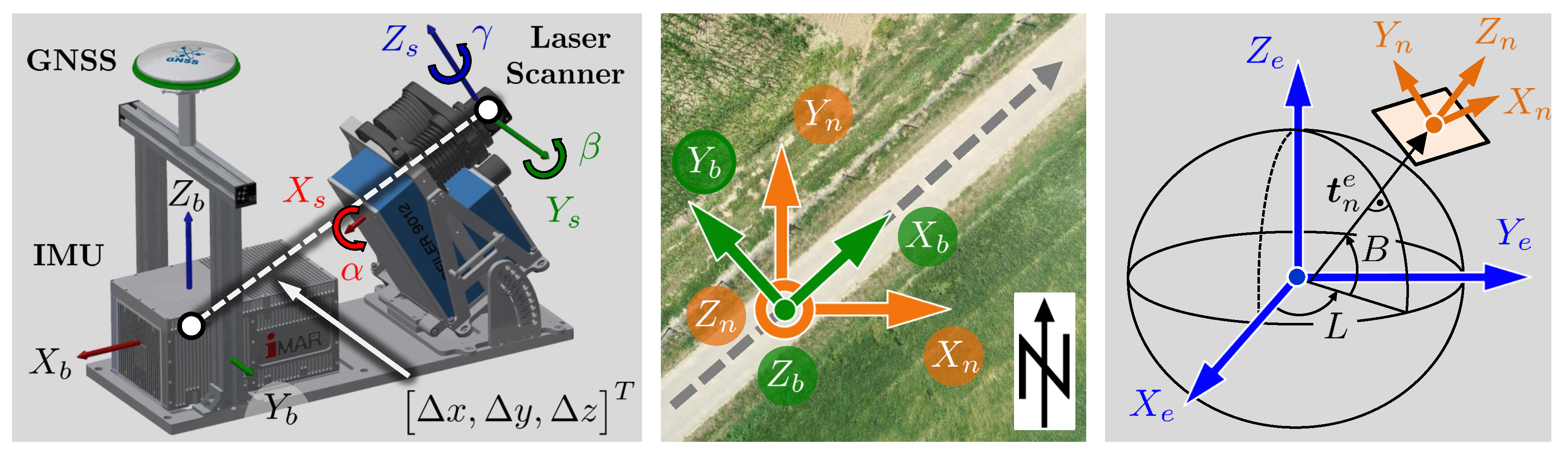
4.1. Calibration Parameters and Georeferencing Equation

The measuring of a 3D point cloud using mobile laser scanning is based on the data fusion of multiple sensors. The goal of the extrinsic calibration is to determine the mutual installation position and orientation of these sensors on the platform. In this paper, we address the determination of the lever arm ${\left[\Delta x,\Delta y,\Delta z\right]}^T$ as well as the boresight angles $\alpha$, $\beta$, and $\gamma$ of a 2D laser scanner w.r.t. a GNSS/IMU unit (Figure 2, left). The calibration approach in Section 4.2 aims at determining these parameters, which are assumed to be temporally constant. However, this has to be checked regularly.

In the context of mobile laser scanning, an object point ${\left[x_s,y_s,z_s\right]}^T$ in the local sensor frame of the 2D laser scanner (s-frame) can be written as ${\left[0,d_s·sin\left(b_s\right),d_s·cos\left(b_s\right)\right]}^T$, where $d_s$ is the measured distance and $b_s$ the scanning angle. In order to obtain a georeferenced point cloud, the object points of the 2D laser scanner must be transformed into the body-frame of the platform (b-frame), which often coincides with the coordinate system of the IMU. For this transformation, the extrinsic calibration parameters are needed, i.e., the lever arm ${\left[\Delta x,\Delta y,\Delta z\right]}^T$ as well as the boresight angles $\alpha$, $\beta$, and $\gamma$ (Figure 2, left). Subsequently, the orientation angles of the platform, i.e., roll $\varphi$, pitch $\theta$, and yaw $\psi$, are used to transform the object points into the navigation-frame (n-frame), which is a north-oriented local level frame, whose origin coincides with that of the b-frame (Figure 2, middle). Finally, the object points are transformed to a superordinate earth-fixed and earth-centered coordinate frame, which we denote as e-frame (Figure 2, right), by using ellipsoidal longitude L and latitude B, as well as the translation vector ${\mathit{t}}_n^e={\left[t_x,t_y,t_z\right]}^T$. All these transformations can be combined to the georeferencing equation, which provides georeferenced scan points ${\left[x_e,y_e,z_e\right]}_{MLS}^T$ (MLS: Mobile Laser Scanning):

$${\left[\begin{array}{c}{x}_e\\ y_e\\ z_e\end{array}\right]}_{MLS}=\left[\begin{array}{c}{t}_x\\ t_y\\ t_z\end{array}\right]+{\mathit{R}}_n^e(L,B)·{\mathit{R}}_b^n(\varphi ,\theta ,\psi )·\left({\mathit{R}}_s^b(\alpha ,\beta ,\gamma )\left[\begin{array}{c}\begin{array}{c}{x}_s=0\hfill \\ y_s=d_s·sin\left(b_s\right)\hfill \\ z_s=d_s·cos\left(b_s\right)\hfill \end{array}\end{array}\right]+\left[\begin{array}{c}\Delta x\\ \Delta y\\ \Delta z\end{array}\right]\right),$$

(1)

where ${\mathit{R}}_i^j(·)$ denotes an Euler rotation matrix between two frames i and j. Afterwards, the global Cartesian coordinates ${\left[x_e,y_e,z_e\right]}_{MLS}^T$ are often transformed to application-related coordinate frames, e.g., UTM (Universal Transverse Mercator) and ellipsoidal heights. In the case of small areas, it is also possible to transform the object points from the n-frame to a local frame (l-frame) by omitting the rotation matrix ${\mathit{R}}_n^e(L,B)$ with ellipsoidal longitude L and latitude B, and just using the translation vector ${\mathit{t}}_n^l={\left[t_e,t_n,t_h\right]}^T$. This leads to the simplified equation:

$${\left[\begin{array}{c}{x}_l\\ y_l\\ z_l\end{array}\right]}_{MLS}=\left[\begin{array}{c}{t}_e\\ t_n\\ t_h\end{array}\right]+{\mathit{R}}_b^n(\varphi ,\theta ,\psi )·\left({\mathit{R}}_s^b(\alpha ,\beta ,\gamma )\left[\begin{array}{c}\begin{array}{c}{x}_s=0\hfill \\ y_s=d_s·sin\left(b_s\right)\hfill \\ z_s=d_s·cos\left(b_s\right)\hfill \end{array}\end{array}\right]+\left[\begin{array}{c}\Delta x\\ \Delta y\\ \Delta z\end{array}\right]\right).$$

(2)

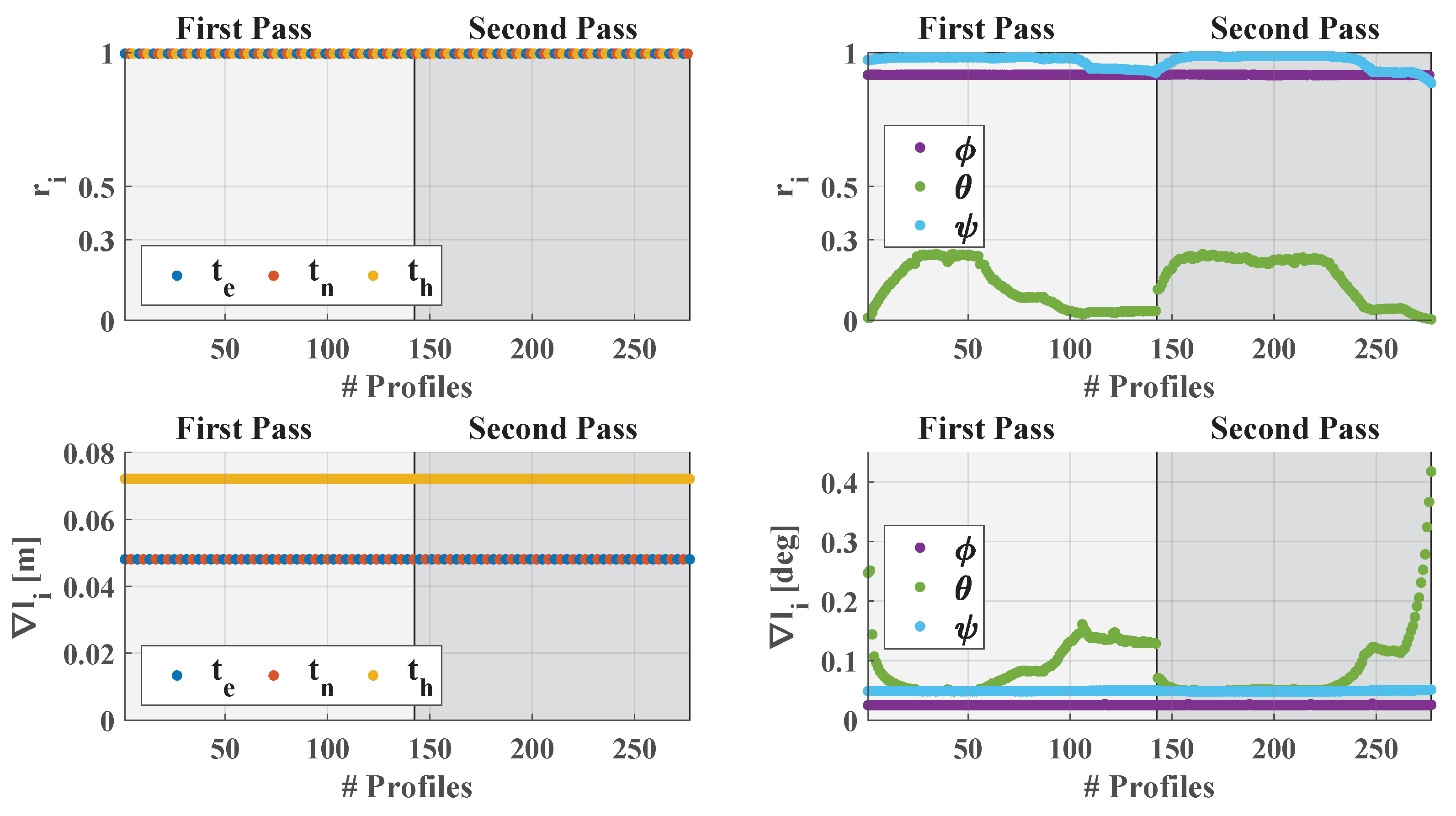
4.2. Calibration Procedure

The calibration approach is based on the use of reference planes [7]. In this section, we describe the calibration procedure with a given plane setup. Yet, we are not interested in how this plane setup was derived. The design of the plane setup and the influence of its configuration on the quality of the estimated calibration parameters are discussed in Section 5. The general workflow of the calibration procedure is illustrated in Figure 3.

The first step of the calibration comprises the determination of reference values for the plane setup (Figure 3, left column). Therefore, the plane setup is scanned with TLS from several stations. The resulting TLS point cloud is georeferenced in the e-frame or l-frame using control points. As a result, each plane is represented by a number of georeferenced points ${\left[x_e,y_e,z_e\right]}_{TLS}^T$. Subsequently, the georeferenced TLS points are approximated with a plane model, which is parameterized by the normal vector ${\left[n_x,n_y,n_z\right]}^T$ and the distance parameter $d_n$. By normalizing the normal vector with $d_n$, the plane equation is described by only three parameters ${\left[{\overline{n}}_x,{\overline{n}}_y,{\overline{n}}_z\right]}^T$ [71]:

$${\left[\begin{array}{c}{x}_e,y_e,z_e\end{array}\right]}_{TLS}·\left[\begin{array}{c}{n}_x\\ n_y\\ n_z\end{array}\right]-d_n={\left[\begin{array}{c}{x}_e,y_e,z_e\end{array}\right]}_{TLS}·\left[\begin{array}{c}{\overline{n}}_x\\ {\overline{n}}_y\\ {\overline{n}}_z\end{array}\right]-1\stackrel{!}{=}0.$$

(3)

The estimated normal vectors ${\left[{\overline{n}}_x,{\overline{n}}_y,{\overline{n}}_z\right]}^T$ serve as reference information for the calibration of the mobile laser scanning system.

Following this, the plane setup is scanned with the mobile laser scanning system (Figure 3, right column). By using the georeferencing equation and approximate calibration parameters, a mobile point cloud of the plane setup in the e-frame or l-frame is calculated (cf. Equation (1) or Equation (2)). The calibration approach is based on the constraint that the georeferenced points ${\left[x_e,y_e,z_e\right]}_{MLS}$ of the mobile laser scanning system must fulfill the plane equations as given from the TLS survey in Equation (3). This leads to the following observation equation for the calibration:

$$\underset{\begin{array}{c}{\left[x_e,y_e,z_e\right]}_{MLS}^T\end{array}}{\underbrace{{\left[\left[\begin{array}{c}{t}_x\\ t_y\\ t_z\end{array}\right]+{\mathit{R}}_n^e(L,B)·{\mathit{R}}_b^n(\varphi ,\theta ,\psi )·\left({\mathit{R}}_s^b(\alpha ,\beta ,\gamma )\left[\begin{array}{c}0\\ d_s·sin{b}_s\\ d_s·cos{b}_s\end{array}\right]+\left[\begin{array}{c}\Delta x\\ \Delta y\\ \Delta z\end{array}\right]\right)\right]}^T}}·\left[\begin{array}{c}{\overline{n}}_x\\ {\overline{n}}_y\\ {\overline{n}}_z\end{array}\right]-1\stackrel{!}{=}0.$$

(4)

Equation (4) leads to a system of equations that can be solved using a Least Squares adjustment within the Gauß-Helmert Model [15]. In the adjustment, the plane normals ${\left[{\overline{n}}_x,{\overline{n}}_y,{\overline{n}}_z\right]}^T$ are considered as an error-free reference. However, it is also possible to use them as observations when introducing an adequate variance information. The observations in the adjustment are the positions ${\left[t_x,t_y,t_z\right]}^T$ and the orientation angles $\varphi$, $\theta$, and $\psi$ of the mobile laser scanning system, as well as the distances $d_s$ and the angular observations $b_s$ of the 2D laser scanner. The lever arm ${\left[\Delta x,\Delta y,\Delta z\right]}^T$ and the boresight angles $\alpha$, $\beta$, and $\gamma$ are the parameters to be estimated. For small areas the ellipsoidal longitude L and latitude B can be considered as error-free constant values. In the case of performing the parameter estimation in the l-frame, the leveled positions ${\left[t_e,t_n,t_h\right]}^T$ are used as observations.

Please note that not each scan point of the mobile laser scanning system is assigned an own position and orientation, but all scan points within the same scanning profile are assigned the mean position and orientation of that scanning profile. This is reasonable for several reasons:

(i)

Significant reduction of the normal equation system enhancing the computational efficiency,

(ii)

Position and orientation of adjacent scan points are highly correlated and, thus, do not provide a new and independent information,

(iii)

Errors that might be induced by this simplification are negligible due to the high profile rate of the 2D laser scanner, the low speed of the platform, and the accuracy of the trajectory (e.g., at a speed of 0.75 $\frac{\mathrm{m}}{\mathrm{s}}$ and a profile rate of 200 Hz, the maximum position error is < 1 mm).

In order to assign each scan point of the mobile laser scanning to the correct reference plane, the scan lines of the mobile laser scanning system are separately pre-processed. Please note that the pre-processing is not done on the full 3D point cloud of the mobile laser scanning system, but on individual scan lines. This is illustrated in Figure 3 (right column). Initially, the scan lines are given in the s-frame of the 2D laser scanner. By ignoring the $X_s$-component, a 2D scan is obtained, where the planes are represented as line segments. These line segments are extracted from the scan lines by using a RANSAC (Random Sample Consensus) approach [72]. In the RANSAC approach, thresholds for the maximum distance of a scanned point to a line segment as well as for the minimum size of a line segment are used. The thresholds were empirically determined based on the noise of the 2D laser scanner and the known size of the reference planes. Subsequently, the extracted line segments are transformed to the e-frame or l-frame by using the georeferencing equation and approximate calibration parameters (cf. Equation (1) or Equation (2)). Finally, the extracted line segments are inserted into the reference plane equations from TLS and assigned to the plane that gives the minimum distance error. This results in a segmented point cloud of the mobile laser scanning system (Figure 3, bottom right).

4.3. Quality Criteria for the Estimation of the Calibration Parameters

The basic equation of the calibration approach is Equation (4), which is used as an observation equation for a Least Squares adjustment within the Gauß-Helmert model [15]. By using Equation (5) and Equation (6), the calibration parameters $\widehat{\mathit{p}}={\left[\Delta x,\Delta y,\Delta z,\alpha ,\beta ,\gamma \right]}^T$ and their covariance matrix ${\mathsf{\Sigma }}_{\widehat{p}\widehat{p}}$ can be estimated, respectively:

$$\widehat{\mathit{p}}={\mathit{p}}_0+{\left[{\mathit{A}}^T{\left(\mathit{B}{\mathsf{\Sigma }}_{ll}{\mathit{B}}^T\right)}^{-1}\mathit{A}\right]}^{-1}{\mathit{A}}^T{\left(\mathit{B}{\mathsf{\Sigma }}_{ll}{\mathit{B}}^T\right)}^{-1}\mathit{w},$$

(5)

$${\mathsf{\Sigma }}_{\widehat{p}\widehat{p}}={\left[{\mathit{A}}^T{\left(\mathit{B}{\mathsf{\Sigma }}_{ll}{\mathit{B}}^T\right)}^{-1}\mathit{A}\right]}^{-1},$$

(6)

where ${\mathit{p}}_0$ denotes approximate calibration parameters, the matrizes $\mathit{A}$ and $\mathit{B}$ contain the partial derivatives of Equation (4) w.r.t. the parameters and observations, respectively, ${\mathsf{\Sigma }}_{ll}$ is the covariance matrix of the observations and $\mathit{w}$ is the vector of discrepancies. The covariance matrix ${\mathsf{\Sigma }}_{\widehat{p}\widehat{p}}$ indicates the accuracy of the estimated calibration parameters $\widehat{\mathit{p}}$ and is an important criterion for analyzing the quality of the calibration parameters. The main goal of the calibration is that the uncertainty of the 3D point cloud, which is principally caused by the observation errors of the GNSS/IMU unit and the 2D laser scanner, does not increase significantly by the uncertainty ${\mathsf{\Sigma }}_{\widehat{p}\widehat{p}}$ of the calibration.

In order to define a target accuracy for the estimated calibration parameters, we performed an error propagation of Equation (2) with optimistic assumptions for the accuracy of the observations. These accuracies were oriented towards empirical values and manufacturer specifications and are summarized in

Table 1. Standard deviations for the error propagation of the georeferencing equation (Equation (2)).

	Position		Orientation		2D Laser Scanner		Calibration Parameters
	${\mathit{t}}_{\mathit{e}}$, ${\mathit{t}}_{\mathit{n}}$	${\mathit{t}}_{\mathit{h}}$	$\mathit{\varphi }$, $\mathit{\theta }$	$\mathit{\psi }$	${\mathit{d}}_{\mathit{s}}$	${\mathit{b}}_{\mathit{s}}$	$\mathbf{\Delta }\mathit{x}$, $\mathbf{\Delta }\mathit{y}$	$\mathbf{\Delta }\mathit{z}$	$\mathit{\alpha }$, $\mathit{\beta }$, $\mathit{\gamma }$
(i) Obs	0.01 m	0.015 m	0.005${}^{\circ }$	0.010${}^{\circ }$	0.001 m	0.005${}^{\circ }$	–	–	–
(ii) Obs + Cal	0.01 m	0.015 m	0.005${}^{\circ }$	0.010${}^{\circ }$	0.001 m	0.005${}^{\circ }$	0.001 m	0.0015 m	0.005${}^{\circ }$

. Two different scenarios were simulated, i.e., with and without an uncertainty for the calibration parameters. In Table 1, these two scenarios are denoted with cases (i) and (ii). The error propagation was executed in a local frame (l-frame) with east, north, and height component in order to distinguish between horizontal and vertical accuracy. A point grid was generated for the scan profile of the 2D laser scanner with a typical operating range of 50 m. For each grid point, a covariance matrix was calculated via error propagation. Based on this, a 3D point error ${\sigma }_{3D}=\sqrt{{\sigma }_{x_l}^2+{\sigma }_{y_l}^2+{\sigma }_{z_l}^2}$ was derived from the trace of each covariance matrix.

Figure 4 (left) visualizes the 3D point errors ${\sigma }_{3D}^{obs}$ based on observation errors only (cf. Table 1, case (i)). In the close range, position errors are dominant with about 20 mm. Because of orientation errors, the uncertainty increases at higher distances. Figure 4 (right) shows the additional uncertainty of the point cloud when an uncertainty for the calibration parameters is added, i.e., ${\sigma }_{3D}^{add}={\sigma }_{3D}^{obs+cal}-{\sigma }_{3D}^{obs}$ (cf. Table 1, case (ii) – case (i)). A radially symmetrical pattern is visible. However, the additional uncertainty is ${\sigma }_{3D}^{add}$ < 1 mm within a radius of 50 m. We define this to be the goal of the calibration. Thus, given optimistic assumptions for the accuracy of the observations, the calibration parameters must be determined with a standard deviation of ≤ 1 ... 1.5 mm for the lever arm and ≤ 0.005${}^{\circ }$ for the boresight angles (cf. Table 1, case (ii)).

Beside the accuracy of the calibration parameters, the controllability of the estimation process is the second important quality criterion. Controllability addresses, if gross errors in the observations can be detected in an outlier test (i.e., internal controllability), and if not, how much undetected gross errors affect the parameter estimation (i.e., external controllability) [14,15]. The internal controllability can be analyzed using partial redundancies $r_i\in [0,1]$, which can be calculated for each observation $l_i$ according to [73,74]:

$$r_i={\left({\mathsf{\Sigma }}_{vv}{\mathsf{\Sigma }}_{ll}^{-1}\right)}_{ii}={\left({\mathsf{\Sigma }}_{ll}{\mathit{B}}^T{\mathsf{\Sigma }}_{\overline{l}\overline{l}}^{-1}\left[\mathbf{I}-\mathit{A}{\left({\mathit{A}}^T{\mathsf{\Sigma }}_{\overline{l}\overline{l}}^{-1}\mathit{A}\right)}^{-1}{\mathit{A}}^T{\mathsf{\Sigma }}_{\overline{l}\overline{l}}^{-1}\right]\mathit{B}\right)}_{ii},$$

(7)

where ${\mathsf{\Sigma }}_{vv}$ is the covariance matrix of the residuals and ${\mathsf{\Sigma }}_{\overline{l}\overline{l}}=\mathit{B}{\mathsf{\Sigma }}_{ll}{\mathit{B}}^T$. Partial redundancies $r_i$ describe the contribution of an observation to the redundancy r of an adjustment, i.e., $\sum r_i=r$. They further indicate the amount of an observation error that is transferred to the own residual $v_i$. Thus, high partial redundancies increase the probability that gross errors are detected. In geodetic network adjustment, values of $r_i$ > 0.3 are recommended [14]. When testing normalized residuals, it is even possible to calculate the minimum detectable outlier $\nabla l_i$ [14,75,76]:

$$\nabla l_i={\delta }_0({\alpha }_T,{\beta }_T)·\frac{{\sigma }_{l_i}}{\sqrt{r_i}},{\sigma }_{l_i}\in {\mathsf{\Sigma }}_{ll},$$

(8)

where ${\delta }_0$ is called non-centrality parameter, which is a function of the type I error probability ${\alpha }_T$ and the type II error probability ${\beta }_T$ (e.g., ${\delta }_0(0.001,0.20)=4.13)$. Based on the minimum detectable outlier $\nabla l_i$, we can calculate the impact $\nabla {\mathit{p}}_i$ of an undetected outlier on the parameter estimation:

$$\nabla {\mathit{p}}_i={\left({\mathit{A}}^T{\mathsf{\Sigma }}_{\overline{l}\overline{l}}^{-1}\mathit{A}\right)}^{-1}{\mathit{A}}^T{\mathsf{\Sigma }}_{\overline{l}\overline{l}}^{-1}\mathit{B}{\left[\begin{array}{c}0,\cdots ,\nabla l_i,\cdots ,0\end{array}\right]}^T.$$

(9)

Both $r_i$ and $\nabla l_i$ in the observation space as well as $\nabla {\mathit{p}}_i$ in the parameter space allow for a rigorous analysis of the controllability of the parameter estimation in terms of gross errors [14,15].

5. Simulation of the Calibration

The configuration of the plane setup has a substantial impact on the quality of the calibration parameters. Therefore, we developed a simulation environment in order to find a plane setup that meets priorly defined quality criteria. For this purpose, we interpret the plane-based calibration as a geodetic network and investigate the parameter estimation process with geodetic quality criteria for both accuracy and controllability (cf. Section 4.3). This strategy is typically applied in geodetic network adjustment [14], but also for, e.g., surface approximation [71], calibration of TLS [77] or measuring arms [78], and VLBI scheduling (Very Long Baseline Interferometry) [79]. Hereinafter, Section 5.1 describes the simulation environment and Section 5.2 analyzes the realized plane setup.

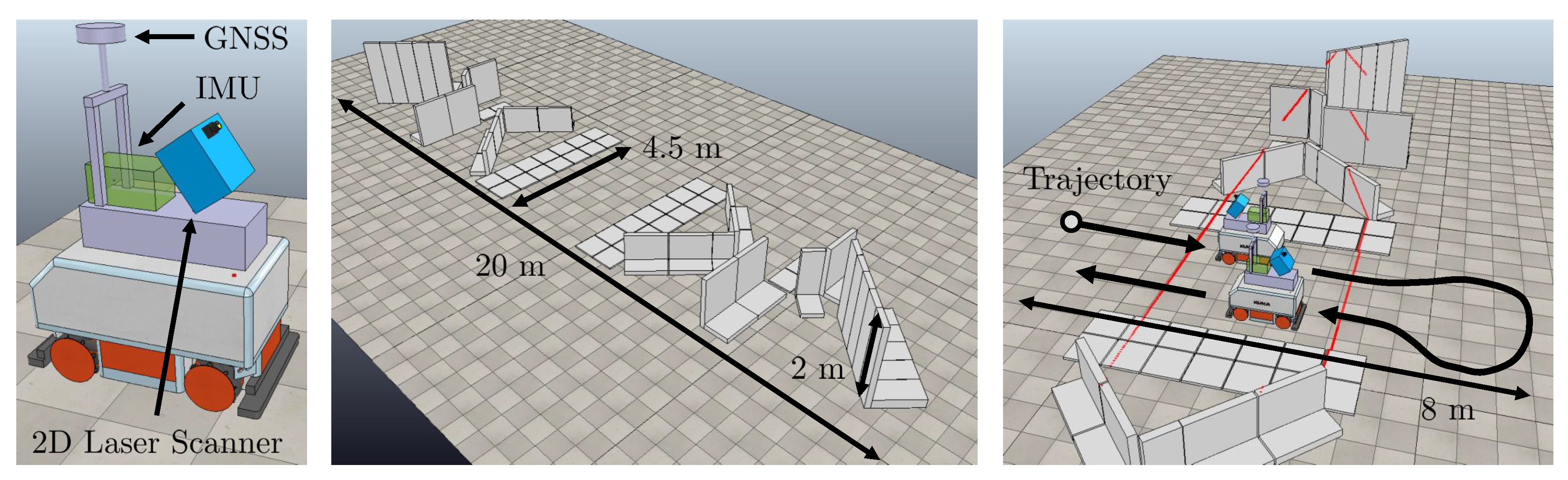
5.1. Simulation Environment

Our simulation environment for the extrinsic calibration of mobile laser scanning systems makes use of the robotic simulation toolbox V-REP (Virtual Robot Experimentation Platform [80]). V-REP enables users to design mobile platforms, which can be equipped with different sensors like GNSS, IMU, laser scanners, or cameras. We utilized V-REP to rebuild the mobile laser scanning system that was introduced in Section 3 (Figure 5, left). In addition to this, V-REP provides the possibility to design environments, in which mobile platforms can operate. Thus, we can also use V-REP to create specific plane setups (Figure 5, middle). Given the mobile laser scanning system and the plane setup, we can simulate the calibration process (Figure 5, right). The plane setup and the simulated sensor observations are then exported to MATLAB (Matrix Laboratory, MathWorks), where we implemented the plane-based calibration approach. In MATLAB, we can analyze and improve the plane setup with quality criteria for both accuracy and controllability (cf. Section 5.2).

A rigorous optimization of the plane setup based on an all-embracing target function is hardly feasible [14,77]. Recently, Hartmann et al. [53] published an approach based on a genetic algorithm in order to optimize the plane configuration for the calibration of a mobile indoor laser scanning system. However, their target function for the optimization of the plane setup is based on the accuracy of the calibration parameters and does not include criteria for the controllability of the parameter estimation. Moreover, boundary conditions for permissible plane setups are required.

In our case, the determination of an appropriate plane setup is based on an iterative refinement of the plane setup. This strategy starts with an educated guess for the plane setup. This educated guess is iteratively refined based on expert knowledge and the quality criteria for both accuracy and controllability of the calibration parameters as introduced in Section 4.3. The iteration is stopped when the calibration parameters meet priorly defined requirements. In addition, we also specify boundary conditions for the plane setup in the calibration field that result from practical reasons:

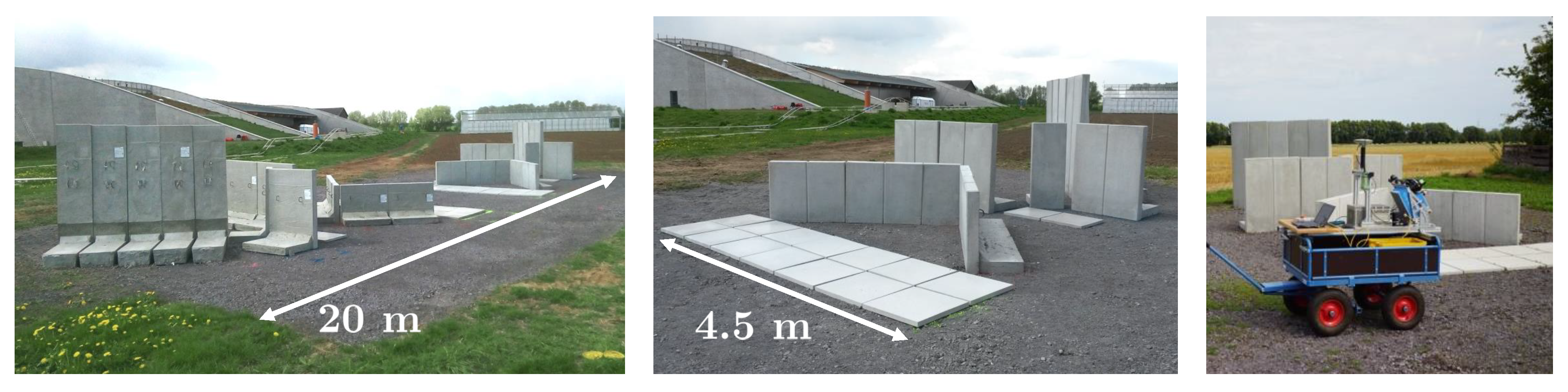
• available area for the calibration field is 10 m × 20 m (cf. Figure 5, middle and right),
• fast and simple calibration procedure for mobile laser scanning systems (cf. Figure 5, right),
• for the reference planes we want to use standard face concrete elements as used for retaining walls in civil engineering (cf. Figure 5 and Section 6.1); such face concrete elements are highly planar, cost-effective, stable, and sufficiently robust for a permanent outdoor installation.

5.2. Simulation Results

This section presents the simulation results of the plane setup in Figure 5, which was finally realized in the calibration field (Section 6.1). This plane setup is scanned with the mobile laser scanning system in two passes. The difference between first and second pass is that the orientation of the system has been turned by 180${}^{\circ }$ (Figure 5, right). The investigation of the plane setup and the calibration procedure can be split into three parts. We start with analyzing the sensitivity of the plane setup w.r.t. the calibration parameters, i.e., how changes of the lever arm and boresight angles affect the consistency between the reference planes and the point cloud of the mobile laser scanning system. This is connected to the separability of the calibration parameters (Section 5.2.1). Following this, we examine the impact of random and systematic observation errors on the precision and accuracy of the estimated calibration parameters (Section 5.2.2). Finally, we investigate the controllability of the parameter estimation, i.e., its robustness w.r.t. gross observation errors (Section 5.2.3).

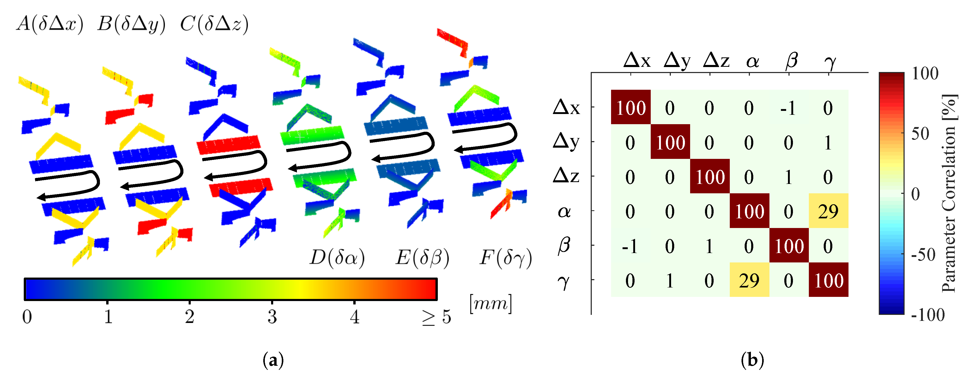
5.2.1. Sensitivity of the Plane Setup and Separability of the Calibration Parameters

In this section, we examine the sensitivity of the plane setup w.r.t. changes in the calibration parameters. Figure 6a depicts the point-to-plane distances of the plane setup when the calibration parameters deviate from their true values by either 5 mm (lever arm) or 0.05${}^{\circ }$ (boresight angles).

For the lever arm components (A, B, C), there is always a subset of planes that is sensitive towards the parameter deviation. For instance, the planes that are inclined by 45${}^{\circ }$ w.r.t. the direction of motion of the platform have a sensitivity of 70% towards changes in $\Delta x$ and $\Delta y$ (yellow color in A and B). In addition, the reference planes that are parallel to the direction of motion are fully sensitive towards changes in $\Delta y$ (red color in B). The planes on the ground are fully sensitive towards changes in $\Delta z$ (red color in C). Regarding the boresight angles, the plane setup has a sufficient sensitivity towards changes in $\alpha$ (D) and $\gamma$ (F), but is less sensitive towards changes in $\beta$ (E). The lower sensitivity towards $\beta$ means that it is more difficult to estimate this parameter based on the minimization of point-to-plane distances like it is done in the calibration. This is proved by both the simulation results (Figure 7) and the results based on real data (Section 6.2), because in both cases the boresight angle $\beta$ has the biggest standard deviation of all boresight angles. The sensitivity towards $\beta$ could be improved by mounting the mobile laser scanning system on a high van. In this case, the distance between the mobile laser scanning system and the ground planes, which are most sensitive towards $\beta$, is increased.

In Figure 6a, we can see that different parameter deviations lead to different patterns of the point-to-plane distances. Thus, making the assumptions that we have no other sources of errors, we can separate erroneous calibration parameters by analyzing their unique deviation patterns. This indicates a good separability of the calibration parameters. The good separability of the calibration parameters is verified by their correlation matrix in Figure 6b, which is derived from the covariance matrix ${\mathsf{\Sigma }}_{\widehat{p}\widehat{p}}$ of the parameter estimation (cf. Equation (6)). According to the correlation matrix, the calibration parameters are basically uncorrelated, except for a small correlation of 29% between the boresight angles $\alpha$ and $\gamma$. The reason for this correlation is the sequence of boresight rotations using Euler angles. Due to the $\beta$ = 30${}^{\circ }$ tilt of the 2D laser scanner (cf. Figure 2, left), the horizontal projection of the $X_s$-axis is smaller than the length of the $X_s$-axis. In the extreme case of $\beta$ = 90${}^{\circ }$, the projection is zero. In navigation, this phenomenon is known as gimbal lock [24], where the boresight angles $\alpha$ and $\gamma$ rotate around the same axis and cannot be separated from each other (100 % correlation). Thus, in the case of $\beta$ = 0${}^{\circ }$, the correlation between $\alpha$ and $\gamma$ is 0 % as is demonstrated in [11]. In our case, the 2D laser scanner is tilted by $\beta$ = 30${}^{\circ }$ and, thus, the correlation is between 0 % and 100 %.

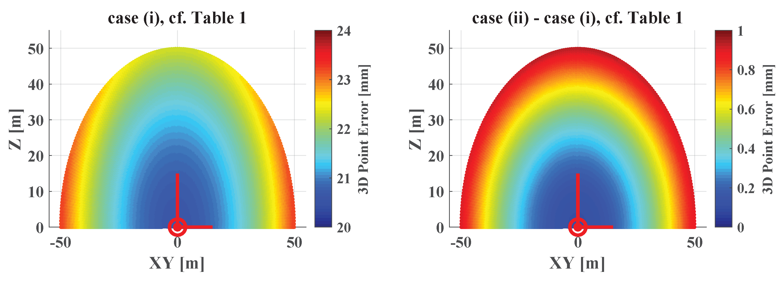
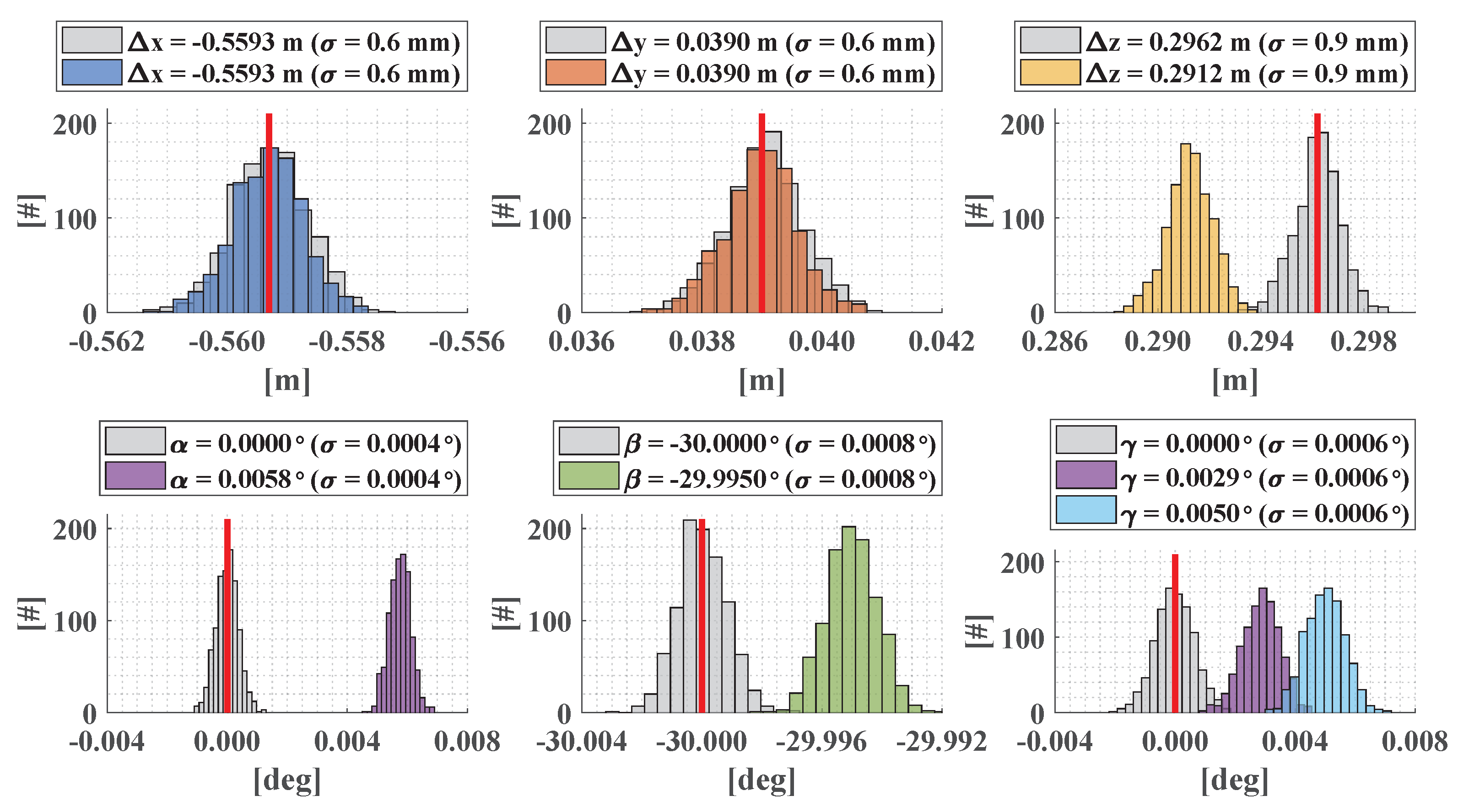
5.2.2. Impact of Random and Systematic Observation Errors

In order to examine how random observation errors of the mobile laser scanning system affect the parameter estimation, we carried out a Monte Carlo simulation with 1000 realizations of the calibration process. Given the plane setup, true calibration parameters, and the observations of the mobile laser scanning system, the noise of the observations was sampled from a Gaussian distribution. The associated standard deviations were oriented towards manufacturer information and empirical values (cf. Table 1). The Monte Carlo simulation was performed in a local frame (l-frame) with east, north, and height component. This allows for a better interpretation of the simulation results. As a result, 1,000 realizations for the estimated calibration parameters $\widehat{\mathit{p}}={\left[\Delta x,\Delta y,\Delta z,\alpha ,\beta ,\gamma \right]}^T$ and their covariance matrix ${\mathsf{\Sigma }}_{\widehat{p}\widehat{p}}$ were obtained. According to Förstner and Wrobel (chap. 4.6.8, pp. 139–141) [15], the unbiasedness of $\widehat{\mathit{p}}$ and ${\mathsf{\Sigma }}_{\widehat{p}\widehat{p}}$ within the simulation can be checked by different statistical tests. All simulations passed these tests.

The grey histograms in Figure 7 show the distributions of the calibration parameters after the Monte Carlo simulation based on random observation errors only. The red vertical lines indicate the true calibration parameters, i.e., the expectation values. It can be stated that all parameters are unbiased if only random observation errors are simulated. For the three lever arm components, a standard deviation of $\sigma$ < 1 mm is obtained. These results meet the defined target accuracies of 1 mm for $\Delta x$ and $\Delta y$ as well as 1.5 mm for $\Delta z$ (cf. Table 1). The accuracy of the lever arm mainly depends on the accuracy of the position ${\left[t_e,t_n,t_h\right]}^T$ of the mobile laser scanning system. The higher standard deviation of $\Delta z$ results from the higher standard deviation of the height component $t_h$, which is assumed to be 1.5 times the standard deviation of the horizontal position $t_e$ and $t_n$ (cf. Table 1).

For the boresight angles $\alpha$, $\beta$, and $\gamma$, standard deviations of $\sigma$ < 0.001${}^{\circ }$ are obtained, which also meet the defined target accuracy of 0.005${}^{\circ }$ (cf. Table 1). The accuracy of the boresight angles mainly depends on the accuracy of the orientation angles of the mobile laser scanning system. In this regard, $\alpha$ is mostly aligned with the roll angle $\varphi$, $\beta$ is mostly aligned with the pitch angle $\theta$, and $\gamma$ is mostly aligned with the yaw angle $\psi$. Thus, the smaller standard deviation of $\alpha$ as compared to $\gamma$ is expected, since the roll angle is assumed to be more accurate than the yaw angle (cf. Table 1). However, the boresight angle $\beta$ is estimated with the lowest accuracy. At this point, we recall the sensitivity analysis in Section 5.2.1, where we found that the plane setup is less sensitive towards the boresight angle $\beta$. Thus, the higher standard deviation of the boresight angle $\beta$ can be attributed to the lower sensitivity of the plane setup. However, the target accuracy of 0.005${}^{\circ }$ is still achieved.

Inherently, the position and orientation observations of a mobile laser scanning system are prone to systematic errors due to the use of GNSS or uncorrected errors of the IMU. Therefore, we repeated the Monte Carlo simulation with additional biases of 5 mm and 0.005${}^{\circ }$ for the position and orientation observations of the mobile laser scanning system. As in the case of random errors, we found that systematic errors of the position mainly affect the lever arm, while systematic errors of the orientation angles mainly affect the boresight angles. The results of the Monte Carlo simulation with both random and systematic observation errors are visualized as colored histograms in Figure 7.

Clearly, the lever arm components $\Delta x$ and $\Delta y$ remain unbiased in the case of systematic observation errors (cf. Figure 7, top left, top middle). The lever arm components $\Delta x$ and $\Delta y$ mainly depend on the horizontal position $t_e$ and $t_n$ of the mobile laser scanning system. In the simulation, we found that the associated systematic errors $\delta t_e$ and $\delta t_n$ are completely transferred to the residuals of $t_e$ and $t_n$ and, thus, do not affect the parameters. This results from the repeated measurements of the plane setup with opposite direction of motion of the platform (cf. Figure 5, right). Basically, this kind of double measurement can be considered as a measurement in two faces, which is an established strategy in geodesy for the elimination of systematic errors [81]. For the height component, however, the systematic error $\delta t_h$ is not eliminated in this way, which is why the lever arm component $\Delta z$ is biased by 5 mm (Figure 7, top right). For the elimination of a systematic height error $\delta t_h$, the mobile platform would need to measure the plane setup upside down in the second pass.

Systematic orientation errors of the mobile laser scanning system are also not eliminated by the double measurement. A systematic error of the pitch angle $\theta$ is completely transferred to the boresight angle $\beta$, which is biased by 0.005${}^{\circ }$ (Figure 7, bottom middle, green histogram). The same applies to a systematic error of the yaw angle $\psi$, which is completely transferred to the boresight angle $\gamma$ (Figure 7, bottom right, light blue histogram). However, in contrast to this, a systematic error of the roll angle $\varphi$ affects the boresight angles $\alpha$ and $\gamma$ (Figure 7, bottom left and right, purple histograms). This phenomenon is caused by the correlation between the boresight angles $\alpha$ and $\gamma$ (cf. Section 5.2.1 and Figure 6b) and the sequence of the Euler rotations from the n-frame back to the s-frame, i.e., ${\mathit{R}}_b^n\left(\psi \right)$→${\mathit{R}}_b^n\left(\theta \right)$→${\mathit{R}}_b^n\left(\varphi \right)$→${\mathit{R}}_s^b\left(\gamma \right)$→${\mathit{R}}_s^b\left(\beta \right)$→${\mathit{R}}_s^b\left(\alpha \right)$. In the case of a systematic error in the roll angle $\varphi$, this error is partially compensated by the boresight angle $\gamma$ before it reaches the boresight angle $\alpha$ due to the correlation between these two parameters. In contrast to this, a systematic error in the yaw angle $\psi$ can completely be compensated by the boresight angle $\gamma$ before it reaches the boresight angle $\alpha$. Similar considerations can be made for a systematic error in the pitch angle $\theta$.

The simulations indicate that systematic errors in the trajectory estimation corrupt the calibration results. However, such systematic errors are often site- and time-dependent, e.g., in the case of GNSS. This means that if we repeat the calibration multiple times over a certain time period, systematic errors might change in magnitude and sign. In this way, systematic errors could get a more random characteristic and, thus, could be reduced by averaging the calibration results of multiple runs.

Another source of systematic errors, which we have not discussed yet, is the 2D laser scanner. In this respect, we simulated a range finder offset of $d_0$ = 2 mm and analyzed its impact on the calibration parameters. As a result, the range finder offset mainly biases the lever arm components $\Delta x$ (≈0.4 mm) and $\Delta z$ (≈1.4 mm), as well as the boresight angle $\beta$ (≈0.033${}^{\circ }$). However, the used plane setup is sensitive towards a range finder offset. Thus, this intrinsic parameter can be added to the functional model in Equation (4) and estimated as part of the calibration. This is demonstrated in Section 6.3, where we estimate the range finder offset $d_0$ for test purposes based on real data.

Finally, we also took errors of the TLS point cloud into consideration, which is the basis for the determination of the reference plane equations (cf. Equation (3)). In this respect, a global registration error of the TLS point clouds seems to be the most serious problem. Hence, we simulated translation errors of up to 3 mm as well as rotation errors of up to 0.02${}^{\circ }$. We found that errors in the horizontal position of the TLS point cloud as well as tilting errors are filtered out to ≥85% in the calibration, i.e., such errors are transferred to the residuals of the adjustment. As in the case of systematic errors of the horizontal position of the mobile laser scanning system, this results from the repeated measurements of the plane setup with opposite direction of motion of the platform. Registration errors in height and azimuth, however, bias $\Delta z$ and $\gamma$, respectively. In practice, the registration of the TLS point cloud is based on a dense network of highly accurate control points (cf. Section 6.1 and Section 7.1). This provides a high degree of accuracy and controllability. In the light of this, we expect registration errors in height and azimuth to be smaller than the target accuracy for the calibration parameters, i.e., 1 ... 1.5 mm for the lever arm components and 0.005${}^{\circ }$ for the boresight angles.

5.2.3. Impact of Gross Observation Errors

In addition to the accuracy, the quality of the estimated calibration parameters is also determined by the detectability of gross observation errors and the impact of undetected gross observation errors on the parameters. Therefore, we calculated the partial redundancies $r_i$ (cf. Equation (7)) and the minimum detectable outliers $\nabla l_i$ (cf. Equation (8)) of the position and orientation observations of the mobile laser scanning system. The results are visualized in Figure 8.

Figure 8 (left column) shows that the partial redundancies of the position are close to 1 and, thus, well controlled. Gross errors of $\nabla t_{e,n}\ge$ 48 mm for the horizontal position and $\nabla t_h\ge$ 72 mm for the height component can be detected due to the different horizontal and vertical accuracy of the mobile laser scanning system. Undetected gross errors in the position bias the lever arm by $|\nabla {\mathit{p}}_{t_{e,n}}|\le$ 0.17 mm and $|\nabla {\mathit{p}}_{t_h}|\le$ 0.26 mm, respectively (not shown in Figure 8). The boresight angles are not affected by gross errors in the position.

Regarding the orientation (Figure 8, right column), the roll angle $\varphi$ and yaw angle $\psi$ are well controlled with partial redundancies of $r_i\ge$ 0.85. However, the pitch angle $\theta$ is weakly controlled with partial redundancies of $r_i<$ 0.3. This is connected to the lower sensitivity of the plane setup towards the boresight angle $\beta$ (Figure 6, case E), which is mostly aligned with the pitch angle $\theta$. Accordingly, the detectability of gross errors is worse for pitch ($\nabla \theta \ge$ 0.05${}^{\circ }$ – 0.4${}^{\circ }$) than for roll ($\nabla \varphi \ge$ 0.025${}^{\circ }$) and yaw ($\nabla \psi \ge$ 0.05${}^{\circ }$). The impact of undetected gross errors in roll and yaw on the boresight angles is $|\nabla {\mathit{p}}_{\varphi }|\le$ 0.00012${}^{\circ }$ and $|\nabla {\mathit{p}}_{\psi }|\le$ 0.00018${}^{\circ }$, respectively. For the pitch angle, the impact is about two to three times larger with $|\nabla {\mathit{p}}_{\theta }|\le$ 0.00031${}^{\circ }$ (not shown in Figure 8). However, despite the small partial redundancies of the pitch angles, their impact values are very small and do not affect the calibration. The impact of gross errors in the orientation on the lever arm is <40 µm and, thus, negligible.

Due to the high redundancy of the adjustment, the partial redundancies of the 2D laser scanner points are nearly $r_i=1$. Hence, outliers can reliably be detected and do not affect the calibration.

Principally, the observations of the mobile laser scanning system are well controlled, which means that undetected gross errors do not considerably affect the calibration. This controllability is especially important for the position and the yaw angle observations of the mobile laser scanning system, because GNSS—which is prone to gross errors—contributes to these observations.

6. Calibration of the Mobile Laser Scanning System

This section presents empirical calibration results of the mobile laser scanning system that was introduced in Section 3. Section 6.1 describes the calibration measurements, Section 6.2 discusses the lever arm and boresight calibration. In Section 6.3, we address the applicability of the calibration field for estimating the range finder offset as additional intrinsic calibration parameter.

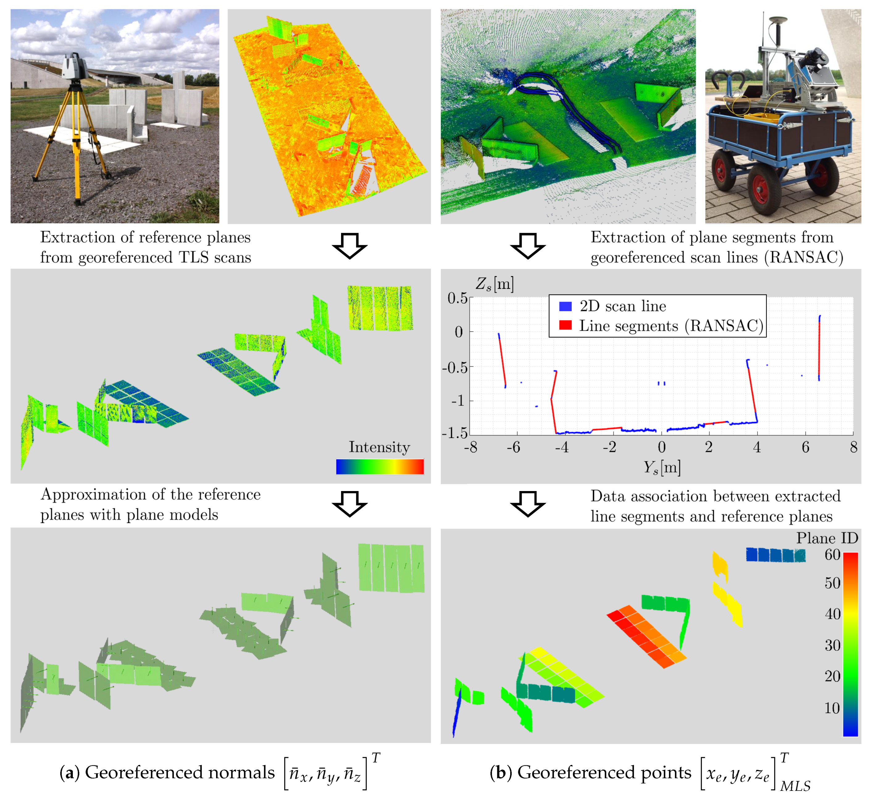
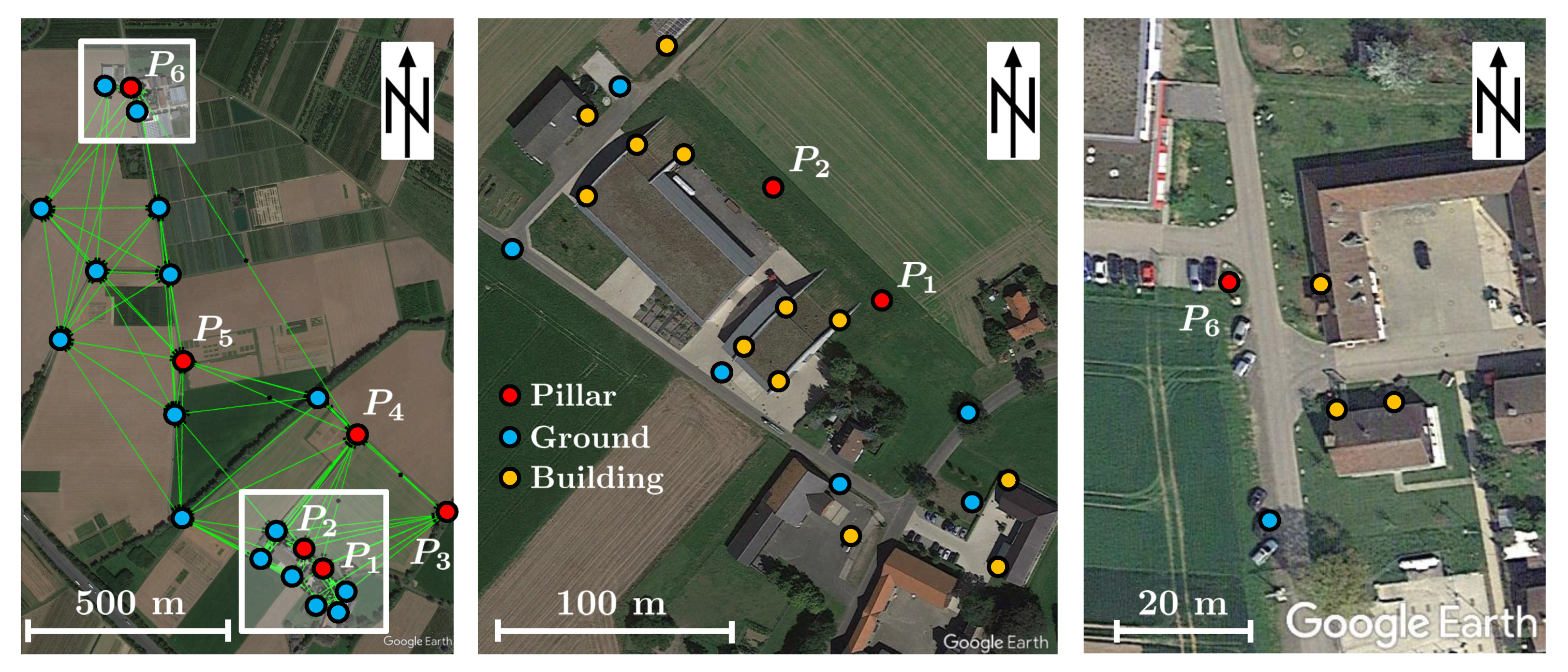
6.1. Calibration Measurements

The plane setup as shown in Figure 5 and validated in Section 5.2 was realized in the form of a permanently installed calibration field. The calibration field is shown in Figure 9. As postulated in Section 5.1, the calibration field covers an area of 10 m × 20 m and was realized using cost-effective, stable, and robust face concrete elements from civil engineering. For the calibration, the system was attached to a trolley due to its easy handling in the calibration field (Figure 9, right).

Initially, reference values for the plane setup were determined with TLS. For this purpose, a Leica ScanStation P50 was set up on five stations in order to completely cover all planes without obstructions. The scans were performed in two faces for reducing systematic errors of the TLS [81]. The TLS point clouds were georeferenced using a network of tie points as well as highly accurate georeferenced control points. All tie and control points were signalized with special BOTA8 targets (Bonn Target 8), which have a square stellar black and white pattern with a size of 0.3 m × 0.3 m (cf. Section 7). The BOTA8 targets have been developed at the University of Bonn and allow for an accurate registration of TLS scans [82]. The mean absolute error after georeferencing was 1.2 mm. Following this, plane models were fitted to the TLS point clouds, which serve as reference information for the calibration. Please note that the control points for the georeferencing of the TLS point clouds are part of a bigger network of control points that was principally realized for the point-based evaluation of the mobile laser scanning systems (cf. Section 7).

For empirically analyzing the quality of the calibration parameters, the calibration procedure as shown in Figure 5 was repeated 98 times. Each calibration run took less than one minute. The 98 runs were performed in four independent blocks with 14, 21, 31, and 32 runs, respectively. After each block, the system was reinitialized. In addition, the blocks were measured at different days and daytimes. That way, different GNSS constellations were covered.

Table 2. Time schedule of the 98 calibration runs, which were measured in July and August 2019.

Block	Date	GPS Time	Runs	Block	Date	GPS Time	Runs
1	31/07/19	01:40 p.m.–01:55 p.m.	14	3	05/08/19	10:30 a.m.–10:50 a.m.	31
2	05/08/19	09:05 a.m.–09:25 a.m.	21	4	05/08/19	11:45 a.m.–12:10 p.m.	32

gives an overview.

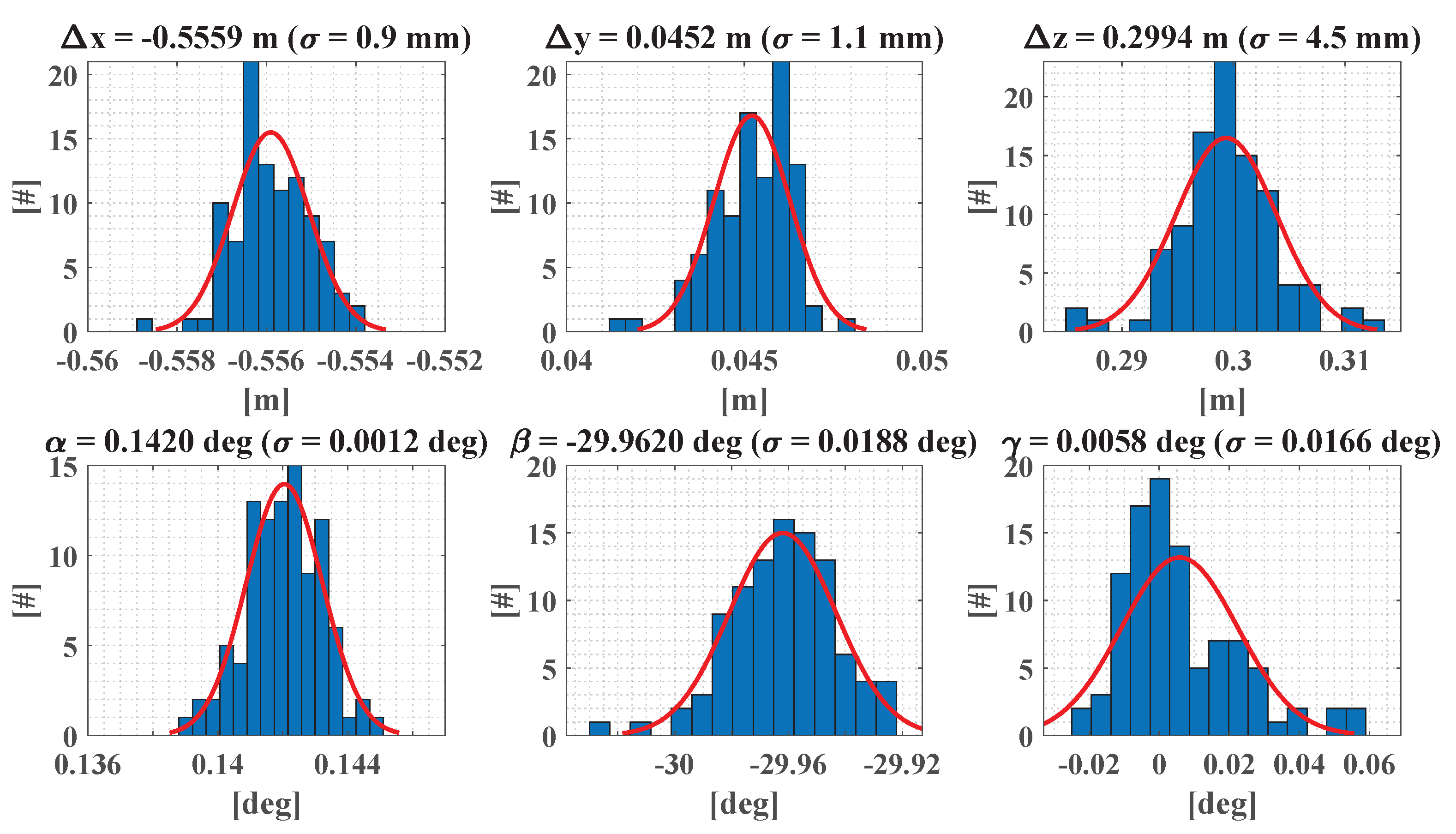
6.2. Calibration of Lever Arm and Boresight Angles

The calibration runs were processed independently. A total of 98 realizations of the calibration parameters were obtained that indicate the repeatability of the calibration. The results are visualized in Figure 10. The mean values and standard deviations are stated on top of the histograms. For better visual assessment, an ideal Gaussian distribution is added to the histograms.

The standard deviations of the lever arm components range from 0.9 mm to 4.5 mm. According to the simulation in Section 5.2, the horizontal components $\Delta x$ and $\Delta y$ are more precise than the vertical component $\Delta z$. This is due to the fact that the quality of the lever arm calibration mainly depends on the accuracy of the position of the GNSS/IMU unit. In the case of GNSS/IMU integration, the height component is normally less accurate than the horizontal component [22,23]. In particular, systematic height errors are critical, since such errors can hardly be detected in the calibration and affect the lever arm component $\Delta z$. In contrast, systematic errors in the horizontal position can be eliminated by measuring the plane setup with opposite direction of motion of the platform (cf. Section 5.2.2). Hence, $\Delta z$ is expected to be worse than $\Delta x$ and $\Delta y$ due to potential systematic height errors. These results are in good accordance with the simulations in Section 5.2. According to the simulations, gross errors in position most likely do not affect the lever arm, since they can reliably be detected.

The standard deviations of the boresight angles range from 0.0012${}^{\circ }$ to 0.0188${}^{\circ }$. According to the simulations, the boresight angle $\beta$ is estimated with the lowest accuracy. This is due to the fact that the plane setup is less sensitive towards $\beta$ than towards $\alpha$ and $\gamma$ (cf. Section 5.2.1). Generally, the accuracy of the boresight angles depends on the accuracy of the orientation angles of the GNSS/IMU unit. While roll and pitch can be estimated from the accelerometers, the yaw determination is more challenging, since it depends on the quality of the initial IMU alignment and the quality of GNSS during motion [23]. In this respect, the yaw angle is more prone to systematic errors than roll and pitch. Basically, systematic errors in the yaw angle affect the boresight angle $\gamma$. In Figure 10, the histograms of the parameters $\alpha$ and $\beta$ appear to be closer to a Gaussian distribution than the histogram of the parameter $\gamma$. This may indicate that systematic errors have affected the determination of $\gamma$.

The standard deviations of the histograms in Figure 10 indicate the precision of one realization of the calibration parameters. Except for the parameter $\Delta x$, $\Delta y$, and $\alpha$, the required target accuracy of 1 ... 1.5 mm for the lever arm as well as 0.005${}^{\circ }$ for the boresight angles as defined in Section 5.2 is not reached. Generally, the empirical standard deviations are higher than those from simulation. This might be caused by systematic errors or neglected correlations that exist in reality, but were not simulated. For n uncorrelated realizations of the calibration parameters, however, the accuracy of the mean value can be improved by $\sqrt{n}$. In our case, 15 statistically independent calibrations are needed to reach the target accuracies for $\Delta z$, $\beta$, and $\gamma$ (

Table 3. Standard deviations for a single calibration run and multiple calibration runs.

Parameter	${\mathit{\sigma }}_{\mathbf{\Delta }\mathit{x}}$	${\mathit{\sigma }}_{\mathbf{\Delta }\mathit{y}}$	${\mathit{\sigma }}_{\mathbf{\Delta }\mathit{z}}$	${\mathit{\sigma }}_{\mathit{\alpha }}$	${\mathit{\sigma }}_{\mathit{\beta }}$	${\mathit{\sigma }}_{\mathit{\gamma }}$
Target Accuracy	1.0 mm	1.0 mm	1.5 mm	0.0050${}^{\circ }$	0.0050${}^{\circ }$	0.0050${}^{\circ }$
1 Realization	0.9 mm	1.1 mm	4.5 mm	0.0012${}^{\circ }$	0.0188${}^{\circ }$	0.0166${}^{\circ }$
15 Realizations	0.2 mm	0.3 mm	1.2 mm	0.0003${}^{\circ }$	0.0049${}^{\circ }$	0.0043${}^{\circ }$
98 Realizations	0.1 mm	0.1 mm	0.5 mm	0.0001${}^{\circ }$	0.0019${}^{\circ }$	0.0017${}^{\circ }$

). Obviously, individual calibration runs are not fully uncorrelated. Therefore, we recommend to perform 15 calibration runs in the calibration field and to repeat this after a break of 1–3 h. After some hours the GNSS constellation is changed, which should lead to different systematic errors in the trajectory estimation.

Figure 11 shows the additional uncertainty ${\sigma }_{3D}^{add}={\sigma }_{3D}^{obs+cal}-{\sigma }_{3D}^{obs}$ of the mobile point cloud that results from the difference between a point cloud that includes an uncertainty of the calibration (${\sigma }_{3D}^{obs+cal}$) and a point cloud that does not include an uncertainty of the calibration (${\sigma }_{3D}^{obs}$); cf. Figure 4 (left). Clearly, the additional uncertainty of the point cloud is ${\sigma }_{3D}^{add}$ < 1 mm within a 50 m radius when using a mean calibration. Please remember that this was the overall goal of the calibration.

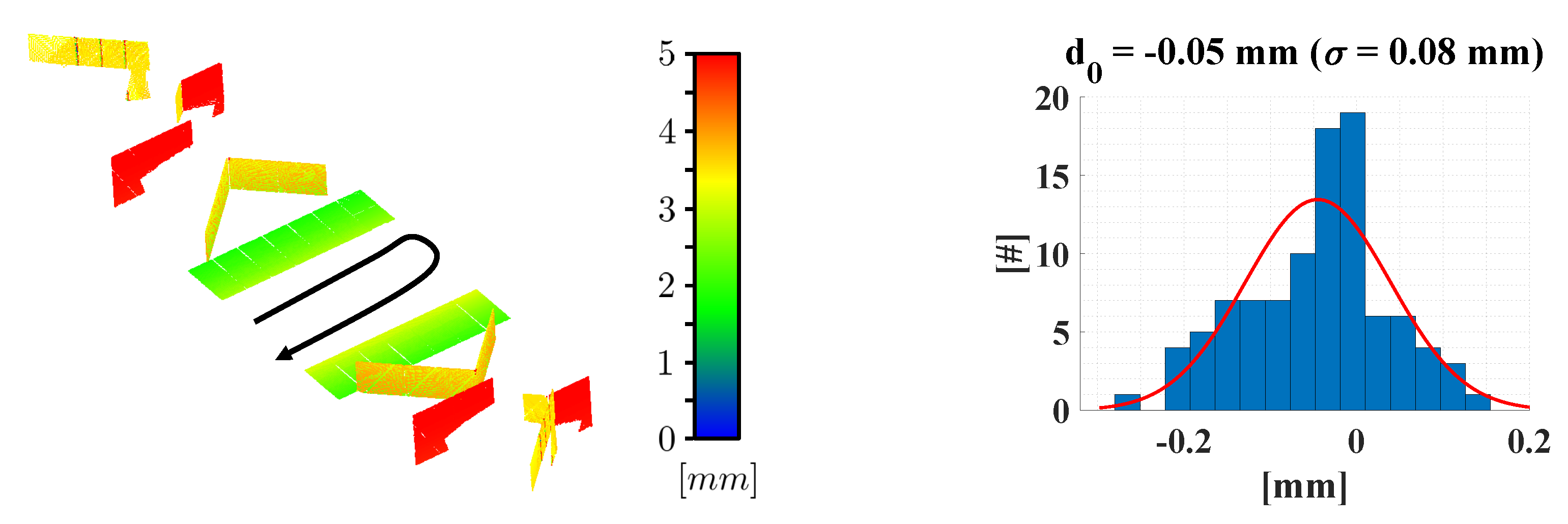
6.3. Calibration of Range Finder Offset

As mentioned in Section 5.2.2, the calibration field is also sensitive towards the range finder offset $d_0$ of the 2D laser scanner. The right part of Figure 12 depicts the sensitivity of the plane setup towards an uncorrected range finder offset of $d_0$ = 5 mm (cf. Figure 6). The range finder offset $d_0$ can simply be added to the calibration model (cf. Equation (4)):

$${\left[\left[\begin{array}{c}{t}_x\\ t_y\\ t_z\end{array}\right]+{\mathit{R}}_n^e(L,B)·{\mathit{R}}_b^n(\varphi ,\theta ,\psi )·\left({\mathit{R}}_s^b(\alpha ,\beta ,\gamma )\left[\begin{array}{c}0\\ (d_s+d_0)·sin{b}_s\\ (d_s+d_0)·cos{b}_s\end{array}\right]+\left[\begin{array}{c}\Delta x\\ \Delta y\\ \Delta z\end{array}\right]\right)\right]}^T·\left[\begin{array}{c}{\overline{n}}_x\\ {\overline{n}}_y\\ {\overline{n}}_z\end{array}\right]-1\stackrel{!}{=}0.$$

(10)

For test purposes, we estimated the range finder offset $d_0$ for each of the 98 calibation runs. The result is shown in the right part of Figure 12. The related histogram has a mean value of −0.05 mm and an empirical standard deviation of 0.08 mm. Accordingly, the range finder offset can be estimated in our calibration field. In this case, however, the range finder offset is of negligible magnitude.

7. Evaluation of the Mobile Laser Scanning System

This section addresses the evaluation of the mobile laser scanning system. In Section 7.1, we introduce the evaluation environment. Section 7.2 describes the evaluation measurements. Based on this, two different evaluation strategies are pursued, i.e., a point-based evaluation using control points (Section 7.3) and an area-based evaluation using TLS reference point clouds (Section 7.4).

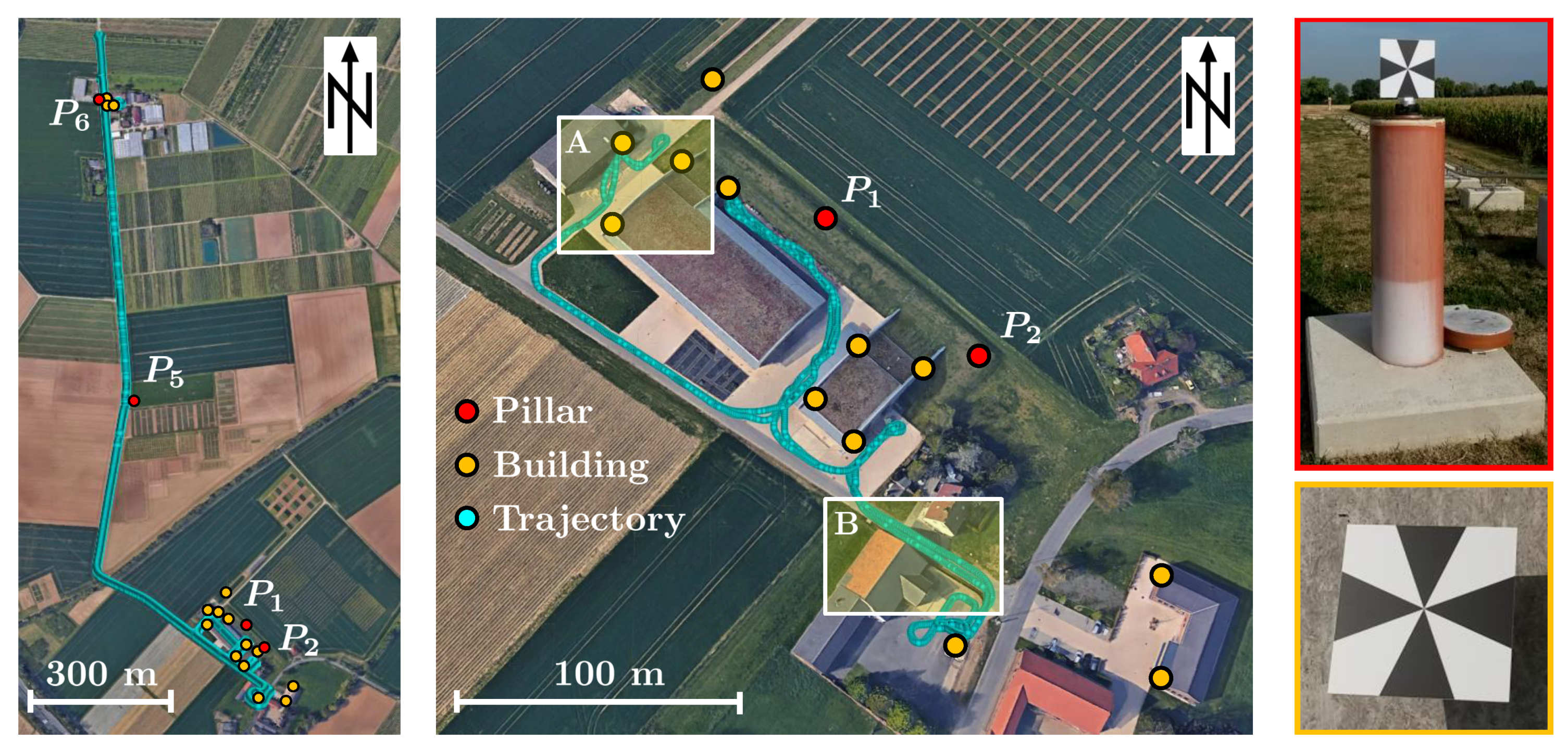
7.1. Evaluation Environment

The evaluation environment contains a network of control points (6 pillars, 16 ground points, 15 building points) that covers an area of about 1.5 km${}^2$ with variable GNSS conditions (Figure 13). The control point coordinates were determined in a network adjustment using measurements from total stations, GNSS baselines, and levelings. The network is linked to the official German coordinate systems, i.e., ETRS89/UTM32 (European Terrestrial Reference System 1989, Universal Transverse Mercator, Zone 32) for position, and DHHN16 (Deutsches Haupthöhennetz 2016) for physical heights. In addition, the ellipsoidal heights w.r.t. GRS80 (Geodetic Reference System 1980) were determined. The connection between the ellipsoidal heights and the physical heights was realized by using the German Combined Quasi Geoid Model (GCG16) [83]. The network was surveyed in June 2017 and July 2018 for checking its stability [84]. The final control point coordinates are based on a combined network adjustment of both epochs and have estimated standard deviations of <1 mm.

In addition to the control points, TLS reference point clouds of all buildings in the area of the control points were measured (Figure 14). The TLS scans were captured from multiple stations in two faces and georeferenced using the network of control points like it was done for the calibration field in Section 6.1. The mean absolute error after georeferencing was 1.2 mm. The TLS reference point clouds can be used for an area-based evaluation of mobile laser scanning systems. In addition, a point-based evaluation is possible based on the control points. For this purpose, the pillars and building points can be signalized with special BOTA8 laser scanning targets [82] (cf. Figure 15), which are applicable to both TLS registration and evaluation of mobile laser scanning systems.

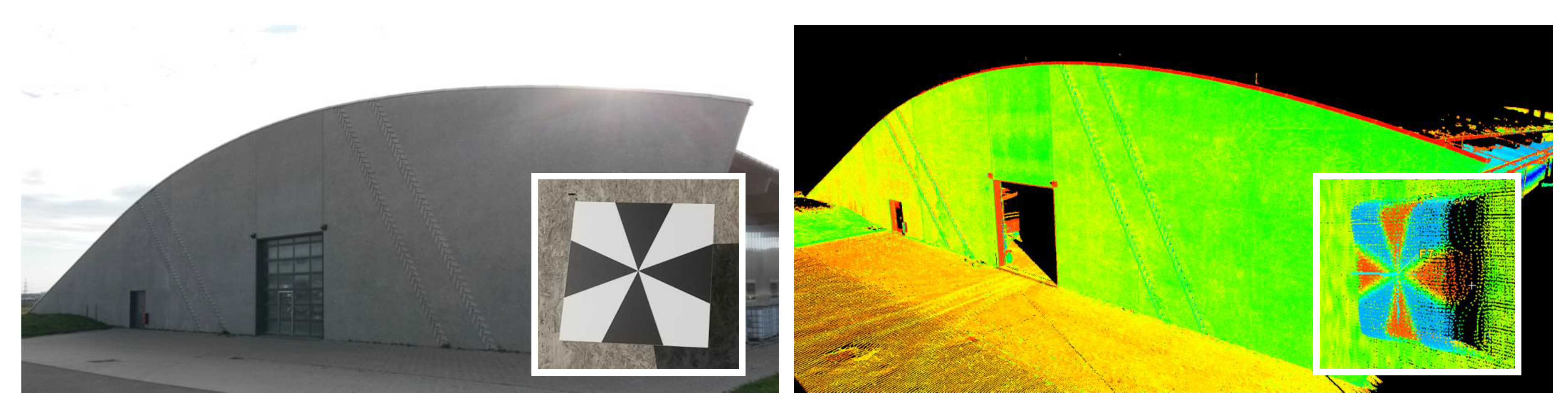
7.2. Evaluation Measurements

For the evaluation of the mobile laser scanning system, five test runs were carried out in November 2018 and August 2019 using both a trolley and a van as carrier platform.

Table 4. Time schedule of the evaluation measurements in November 2018 and August 2019.

Run	Date	GPS Time	Duration	Platform	Covered Distance	Targets
1	13/11/18	09:26 a.m.–09:45 a.m.	18:37 min	Trolley	1250 m	24
2	05/08/19	09:25 a.m.–09:52 a.m.	26:24 min	Trolley	1570 m	31
3	05/08/19	10:50 a.m.–11:15 a.m.	24:28 min	Trolley	1370 m	29
4	05/08/19	12:10 p.m.–12:35 p.m.	24:22 min	Trolley	1330 m	27
5	05/08/19	01:10 p.m.–01:54 p.m.	43:17 min	Van	7990 m	37

gives an overview.

During the test runs, a total distance of 13.5 km was covered. The trajectory was different for each run and lasted between 18 and 43 min. As an example, the cyan dots in Figure 15 indicate the trajectories of run 4 with a trolley and run 5 with a van (cf. Table 4). For each test run, the mobile laser scanning system was reinitialized. For a point-based evaluation, BOTA8 targets were adapted to the control points and scanned with the mobile laser scanning system. Each control point was scanned multiples times leading to a total number of 148 target scans that can be used for a point-based evaluation of the system. For an area-based evaluation using TLS reference point clouds, two selected test sites A and B in the evaluation environment were repeatedly scanned with the mobile laser scanning system (Figure 15). Test site A contains a face concrete wall with dimensions of 9.5 m × 50 m (cf. Figure 14), and test site B is a road passage with houses. The mobile scans of the test sites A and B were also performed during the five test runs in parallel to the scans of the control points.

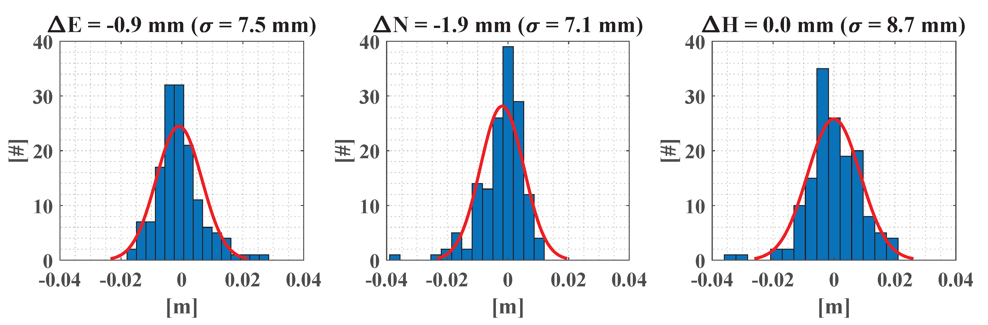
7.3. Point-Based Evaluation Using Control Points

For the point-based evaluation, the coordinates of the control points were extracted from the point clouds of the mobile laser scanning system and compared to the reference values. That way, an evaluation of the entire processing chain including the calibration is possible. Figure 16 shows the histograms of the differences for east, north, and height component for all 148 target scans. An ideal Gaussian distribution is added to the histograms for better visual interpretation. In addition, the mean values $\Delta E$, $\Delta N$, and $\Delta H$ as well as the empirical standard deviations $\sigma$ are stated on top of the histograms. The histograms in Figure 16 have the approximate shape of a Gaussian distribution with absolute mean values of <2 mm and standard deviations of $\sigma$ < 9 mm. The differences between the horizontal and vertical components is marginal. These results indicate a high accuracy of the mobile laser scanning system with a satisfactory extrinsic calibration. Moreover, these results also indicate the high quality of the control points in our evaluation environment.

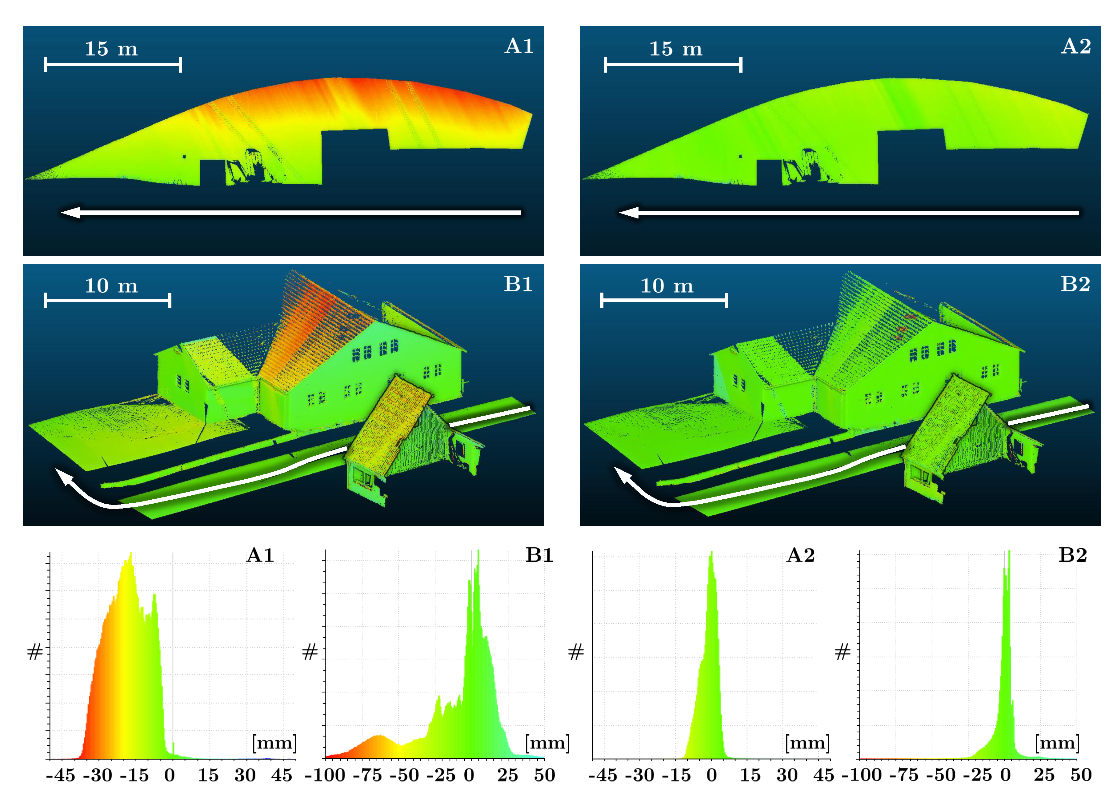
7.4. Area-Based Evaluation Using TLS Reference Point Clouds

For an area-based evaluation, the 3D point clouds of the mobile laser scanning system were compared with TLS reference point clouds. For this purpose, we made use of the M3C2 algorithm (Multiscale-Model-to-Model-Cloud) in the software CloudCompare. The M3C2 algorithm allows for a robust distance computation and comparison between two point clouds [85,86]. Both test sites A and B (cf. Figure 15) were scanned five times with the mobile laser scanning system. In order to demonstrate the potential of an area-based evaluation, we calculated the mobile point clouds with two different sets of calibration parameters, i.e., with an approximate calibration that was taken from the construction plan of the system as well as with the calibration that we determined in our plane-based calibration field. For the plane-based calibration, we utilized the mean values of all 98 calibration runs (cf. Figure 10) as these are the best available calibration parameters.

The results of the area-based evaluation are listed in

Table 5. Area-based evaluation of the mobile laser scanning system using calibration parameters from the construction plan (left) and from the plane-based calibration field (right). The table shows the mean, median, standard deviation (STD), and root mean square error (RMS) of an M3C2 comparison to a TLS reference point cloud. The rows marked with * correspond to the histograms in Figure 17.

	Construction Plan				Plane-Based Calibration Field
Calibration	$\Delta$x = −0.5594 m		$\alpha =\pm {0.0000}^{\circ }$		$\Delta$x = −0.5559 m		$\alpha =+{0.1420}^{\circ }$
Parameters	$\Delta y=+0.0390\mathrm{m}$		$\beta$ = −30.0000${}^{\circ }$		$\Delta y=+0.0452\mathrm{m}$		$\beta$ = −29.9620${}^{\circ }$
	$\Delta z=+0.2962\mathrm{m}$		$\gamma =\pm {0.0000}^{\circ }$		$\Delta z=+0.2994\mathrm{m}$		$\gamma =+{0.0058}^{\circ }$
Test Site	Mean	Median	STD	RMS	Mean	Median	STD	RMS
A	8.7 mm	8.7 mm	8.5 mm	12.2 mm	−6.3 mm	−6.3 mm	4.1 mm	7.6 mm
A *	−18.4 mm	−18.5 mm	8.8 mm	20.4 mm	−1.1 mm	−0.6 mm	4.4 mm	4.5 mm
A	−16.3 mm	−16.2 mm	10.0 mm	19.1 mm	−3.2 mm	−3.5 mm	5.2 mm	6.1 mm
A	−17.5 mm	−17.4 mm	10.1 mm	20.2 mm	−4.4 mm	−5.2 mm	6.3 mm	7.7 mm
A	7.4 mm	7.6 mm	9.1 mm	11.7 mm	3.6 mm	3.5 mm	4.4 mm	5.7 mm
B	1.5 mm	0.3 mm	21.1 mm	21.1 mm	2.5 mm	4.0 mm	8.7 mm	9.0 mm
B *	−9.7 mm	−1.2 mm	27.0 mm	28.7 mm	−0.3 mm	0.6 mm	7.6 mm	7.6 mm
B	−7.9 mm	−2.2 mm	26.2 mm	27.4 mm	0.6 mm	0.7 mm	6.5 mm	6.5 mm
B	−6.9 mm	−2.2 mm	24.9 mm	25.9 mm	−0.7 mm	−0.8 mm	8.3 mm	8.3 mm
B	−14.6 mm	−8.0 mm	30.0 mm	33.4 mm	−4.3 mm	−3.7 mm	8.9 mm	9.9 mm

, which shows the mean, median, standard deviation (STD), and root mean square error (RMS) of the deviations between the mobile point clouds and the TLS reference point clouds that were obtained from the M3C2 comparison. When using the approximate calibration, mean and median values between −18.5 mm and 8.7 mm are obtained (Table 5, left column). In contrast, the plane-based calibration considerably reduces the mean and median values to −6.3 mm to 4.0 mm (Table 5, right column). Thus, the unbiasedness of the point clouds is improved by the plane-based calibration. When using the approximate calibration, we obtain standard deviations and RMS values between 8.5 mm and 33.4 mm. For the plane-based calibration, these values are reduced to 4.1 mm to 9.9 mm. In general, when using the plane-based calibration, the results of the area-based evaluation are in good accordance with the results of the point-based evaluation based on the control points (cf. Figure 16).

Please note that the standard deviations and RMS values are generally smaller in test site A than in test site B. This might be caused by the fact that test site A is not sensitive to all types of errors. In test site A, for example, errors that cause a shift of the mobile point cloud that is parallel to the wall cannot be detected by the M3C2 point cloud comparison. Contrary to this, test site B is more adequate to evaluate the overall system performance, since test site B shows more variation w.r.t. surface position and orientation. This is a drawback of the area-based evaluation strategy using algorithms for the direct comparison of point clouds.

However, the area-based evaluation strategy also carries huge potential for an examination of mobile laser scanning systems. In order to demonstrate this, Figure 17 shows the scatter plots and histograms of the M3C2 point cloud comparison at both test sites A and B for the measurements that are marked with an asterisk (${}^{*}$) in Table 5. A1 and B1 correspond to the approximate calibration taken from the construction plan, and A2 and B2 correspond to the plane-based calibration. At test site A, the mobile laser scanning system was moved parallel to a wall (Figure 17, top row). This wall is also shown in Figure 14. When using the approximate calibration parameters (A1), deviations of up to −40 mm are visible increasing from the bottom up. This pattern indicates a tilting error of the point cloud of the mobile laser scanning system. When using the plane-based calibration (A2), such deviations are vanished. The improvement is also visible in the related histograms. The distribution of A2 is considerably smaller and more unbiased in comparison to A1. When having a closer look to the calibration parameters, which are stated at the beginning of Table 5, we can see that there is a big difference of 0.1420${}^{\circ }$ for the boresight angle $\alpha$. This calibration parameter is mostly aligned with the roll axis of the mobile platform. Hence, the tilting error of the wall in A1 can probably be traced back to an erroneous boresight angle $\alpha$. This example demonstrates that certain errors can be revealed by an area-based evaluation, when using an appropriate object in combination with a specific driving maneuver. This strategy was already proposed in previous publications [34,42,43,44]. However, it is difficult to unambiguously trace back deviations to its origin. For instance, the pattern in A1 could also be caused by an error in the roll angle. In order to clarify this, it would be conceivable to frequently repeat such measurements within a certain period of time making the assumptions that a rolling error is changing, but the calibration error is constant.

Test site A is not sensitive for all kinds of errors, e.g., height errors or errors parallel to the wall. Thus, we extended our investigations to test site B, where the mobile laser scanning system passes a heterogeneous scene with vertical, horizontal, and inclined surfaces (Figure 17, middle row). Test site B is more sensitive to different types of errors and, thus, more adequate to evaluate the mobile laser scanning system. Clearly, the erroneous boresight angle $\alpha$ can be detected at the rooftop (B1). When using the plane-based calibration (B2), the deviations have a mean value of −0.3 mm and a standard deviation of 7.6 mm. Due to the diversity of the scene, such results indicate a satisfactory quality of the calibration parameters. As indicated by the numbers in Table 5 and the histograms in Figure 17, the deviations are not perfectly Gaussian distributed and not completely unbiased, even after applying the plane-based calibration. This is due to the error characteristics of the mobile laser scanning system, which is mostly affected by systematic errors of the trajectory estimation. However, the 2D laser scanner and the M3C2 algorithm also contribute to the error budget.

8. Conclusions and Outlook

This paper presents the design and evaluation of a plane-based calibration field for determining the lever arm and boresight angles of a 2D laser scanner w.r.t. a GNSS/IMU unit on a mobile platform. In addition to this, the calibration field is sensitive for the estimation of the range finder offset of the 2D laser scanner. The calibration field was designed on the basis of a geodetic configuration analysis and Monte Carlo simulations. In this respect, the impact of random, systematic, and gross observation errors on the calibration was analyzed leading to a plane setup that provides accurate and controlled calibration parameters with a standard deviation of ≤1 ... 1.5 mm for the lever arm components and ≤0.005 ${}^{\circ }$ for the boresight angles. This was empirically verified by calibration measurements with our own mobile laser scanning system. Using tools from geodetic configuration analysis to analyze both the accuracy and the controllability of the parameter estimation process in the context of calibrating mobile laser scanning systems has only been addressed to a limited extent so far and is the major scientific contribution of this work. The plane-based calibration field was realized outdoors being permanent, stable, weather-resistant, and cost-effective. The associated calibration procedure in the calibration field takes less than one minute and, thus, can be repeated frequently. In addition to the configuration analysis, repetitive calibrations also increase the controllability of the calibration parameters and allow for a realistic empirical quantification of their accuracy and stability.

In order to evaluate the mobile laser scanning system and the calibration, a dense network of control points and TLS reference point clouds of diverse building structures was installed. These facilities allow for a point-based as well as an area-based evaluation of the overall performance of mobile laser scanning systems. We could demonstrate that the TLS reference point clouds can also partially be utilized to evaluate individual components of the system. Due to the complexity of the systems, however, the evaluation of individual components is challenging. Moreover, the rigorous modeling of the system accuracy by considering an error budget for each component is hardly feasible. Therefore, we argue that an empirical evaluation of the overall system, as conducted within this work, is the most effective strategy. According to our tests, both the point-based and the area-based evaluation indicate that the accuracy of our mobile laser scanning system can be specified with an RMS of <10 mm for the east, the north, and the height component, separately. This accuracy applies to the measuring conditions in our evaluation environment and might change for other fields of applications. Please note that the obtained evaluation results for our mobile laser scanning system are in good accordance with the results that were obtained in a prior case study on a motorway [59].

In the future, we plan to calibrate and evaluate systems other than the one used within this work using our facilities. Moreover, initial tests have been accomplished regarding the expansion of the plane-based calibration field to extrinsic camera calibration (e.g., [87,88,89]).

References

1. Williams, K.; Olsen, M.J.; Gene, V.R.; Glennie, C. Synthesis of Transportation Applications of Mobile LIDAR. Remote Sens. 2013, 5, 4652–4692. [Google Scholar] [CrossRef] [Green Version]
2. Guan, H.; Li, J.; Cao, S.; Yu, Y. Use of mobile LiDAR in road information inventory: A review. Int. J. Image Data Fusion 2016, 7, 219–242. [Google Scholar] [CrossRef]
3. Gargoum, S.A.; El Basyouny, K. A literature synthesis of LiDAR applications in transportation: Feature extraction and geometric assessments of highways. GISci. Remote Sens. 2019, 56, 864–893. [Google Scholar] [CrossRef]
4. Soilán, M.; Sánchez-Rodríguez, A.; del Río-Barral, P.; Perez-Collazo, C.; Arias, P.; Riveiro, B. Review of Laser Scanning Technologies and Their Applications for Road and Railway Infrastructure Monitoring. Infrastructures 2019, 4, 58. [Google Scholar] [CrossRef] [Green Version]
5. Wang, Y.; Chen, Q.; Zhu, Q.; Liu, L.; Li, C.; Zheng, D. A Survey of Mobile Laser Scanning Applications and Key Techniques over Urban Areas. Remote Sens. 2019, 11, 1540. [Google Scholar] [CrossRef] [Green Version]
6. Puente, I.; González-Jorge, H.; Martínez-Sánchez, J.; Arias, P. Review of mobile mapping and surveying technologies. Measurement 2013, 46, 2127–2145. [Google Scholar] [CrossRef]
7. Strübing, T.; Neumann, I. Positions- und Orientierungsschätzung von LIDAR-Sensoren auf Multisensorplattformen. Z. Für Geodäsie Geoinf. Und Landmanag. (ZfV) 2013, 138, 210–221. [Google Scholar]
8. Filin, S. Recovery of Systematic Biases in Laser Altimetry Data Using Natural Surfaces. Photogramm. Eng. Remote Sens. 2003, 69, 1235–1242. [Google Scholar] [CrossRef]
9. Lu, X.; Feng, C.; Ma, Y.; Yang, F.; Shi, B.; Su, D. Calibration method of rotation and displacement systematic error for ship-borne mobile surveying systems. Surv. Rev. 2017, 51, 78–86. [Google Scholar] [CrossRef]
10. Heinz, E.; Eling, C.; Wieland, M.; Klingbeil, L.; Kuhlmann, H. Development, Calibration and Evaluation of a Portable and Direct Georeferenced Laser Scanning System for Kinematic 3D Mapping. J. Appl. Geod. 2015, 9, 227–243. [Google Scholar] [CrossRef]
11. Heinz, E.; Eling, C.; Wieland, M.; Klingbeil, L.; Kuhlmann, H. Analysis of different reference plane setups for the calibration of a mobile laser scanning system. In Ingenieurvermessung 17, Beiträge zum 18. Internationalen Ingenieurvermessungskurs, Graz, Österreich; Lienhart, W., Ed.; Wichmann Verlag: Berlin, Germany, 2017; pp. 131–145. [Google Scholar]
12. Hong, S.; Park, I.; Lee, J.; Lim, K.; Choi, Y.; Sohn, H.G. Utilization of a Terrestrial Laser Scanner for the Calibration of Mobile Mapping Systems. Sensors 2017, 17, 474. [Google Scholar] [CrossRef] [PubMed] [Green Version]
13. Hartmann, J.; Paffenholz, J.A.; Strübing, T.; Neumann, I. Determination of Position and Orientation of LiDAR Sensors on Multisensor Platforms. J. Surv. Eng. 2017, 143. [Google Scholar] [CrossRef]
14. Niemeier, W. Ausgleichungsrechnung—Statistische Auswertemethoden (2., überarbeitete und erweiterte Auflage); de Gruyter: Berlin, Germany; New York, NY, USA, 2008. [Google Scholar]
15. Förstner, W.; Wrobel, B. Photogrammetric Computer Vision—Statistics, Geometry, Orientation and Reconstruction; Springer International Publishing: Cham, Switzerland, 2016. [Google Scholar]
16. Glennie, C. Rigorous 3D error analysis of kinematic scanning LIDAR systems. J. Appl. Geod. 2007, 1, 147–157. [Google Scholar] [CrossRef]
17. Mezian, M.; Vallet, B.; Soheilian, B.; Paparoditis, N. Uncertainty Propagation For Terrestrial Mobile Laser Scanner. Int. Arch. Photogramm. Remote Sens. Spat. Inf. Sci. 2016, 41, 331–335. [Google Scholar] [CrossRef]
18. Hauser, D.; Glennie, C.; Brooks, B. Calibration and Accuracy Analysis of a Low-Cost Mapping-Grade Mobile Laser Scanning System. J. Surv. Eng. 2016, 142, 04016011. [Google Scholar] [CrossRef]
19. Barber, D.; Mills, J.; Smith-Voysey, S. Geometric validation of a ground-based mobile laser scanning system. ISPRS J. Photogramm. Remote Sens. 2008, 63, 128–141. [Google Scholar] [CrossRef]
20. Kaartinen, H.; Hyyppä, J.; Kukko, A.; Jaakkola, A.; Hyyppä, H. Benchmarking the Performance of Mobile Laser Scanning Systems Using a Permanent Test Field. Sensors 2012, 12, 12814–12835. [Google Scholar] [CrossRef] [Green Version]
21. Hofmann, S.; Brenner, C. Accuracy assessment of Mobile Mapping Point Clouds Using the Existing Environment as Terrestrial Reference. Int. Arch. Photogramm. Remote Sens. Spat. Inf. Sci.-ISPRS Arch. 2016, 41, 601–608. [Google Scholar] [CrossRef] [Green Version]
22. Teunissen, P.J.G.; Montenbruck, O. (Eds.) Springer Handbook of Global Navigation Satellite Systems; Springer International Publishing: Cham, Switzerland, 2017. [Google Scholar]
23. Groves, P.D. Principles of GNSS, Inertial, and Multisensor Integrated Navigation Systems, 2nd ed.; Artech House: Boston, MA, USA; London, UK, 2013. [Google Scholar]
24. Vosselman, G.; Maas, H.G. Airborne and Terrestrial Laser Scanning; CRC Press, Whittles Publishing: Dunbeath, Scotland, 2010; ISBN 9781439827987. [Google Scholar]
25. Holst, C.; Neuner, H.; Wieser, A.; Wunderlich, T.; Kuhlmann, H. Calibration of Terrestrial Laser Scanners. Allg. Vermess.-Nachrichten (AVN) 2016, 123, 147–157. [Google Scholar]
26. Gräfe, G. Kinematische Anwendungen von Laserscannern im Straßenraum. Ph.D. Thesis, Gottfried Wilhelm Leibniz Universität Hannover, Fakultät für Bauingenieurwesen und Geodäsie, Hanover, Germany, 2007. [Google Scholar]
27. Brüggemann, T.; Artz, T.; Weiß, R. Kalibrierung von Multisensorsystemen. In Schriftenreihe des DVW, Band 91, Hydrographie 2018 – Trend zu Unbemannten Messsystemen; Wißner Verlag: Augsburg, Germany, 2018; pp. 29–46. [Google Scholar]
28. Hesse, C. Hochauflösende kinematische Objekterfassung mit terrestrischen Laserscannern. Ph.D. Thesis, Gottfried Wilhelm Leibniz Universität Hannover, Fakultät für Bauingenieurwesen und Geodäsie, Hanover, Germany, 2007. [Google Scholar]
29. Vennegeerts, H. Objektraumgestützte kinematische Georeferenzierung für Mobile-Mapping-Systeme. Ph.D. Thesis, ottfried Wilhelm Leibniz Universität Hannover, Fakultät für Bauingenieurwesen und Geodäsie, Hanover, Germany, 2011. [Google Scholar]
30. Eling, C.; Klingbeil, L.; Wieland, M.; Kuhlmann, H. Direct Georeferencing of Micro Aerial Vehicles - System Design, System Calibration and First Evaluation Tests. Photogramm. Fernerkund. Geoinf. (PFG) 2014, 2014, 227–237. [Google Scholar] [CrossRef]
31. Talaya, J.; Alamus, B.; Bosch, E.; Serra, A.; Kornus, W.; Baron, A. Integration of a terrestrial laser scanner with GPS/IMU orientation sensors. In Proceedings of the XXth ISPRS Congress, Istanbul, Turkey, 12–23 July 2004. [Google Scholar]
32. Sheehan, M.; Harrison, A.; Newman, P. Self-calibration for a 3D laser. Int. J. Robot. Res. 2011, 31, 675–687. [Google Scholar] [CrossRef] [Green Version]
33. Elseberg, J.; Borrmann, D.; Nüchter, A. Algorithmic Solutions for Computing Precise Maximum Likelihood 3D Point Clouds from Mobile Laser Scanning Platforms. Remote Sens. 2013, 5, 5871–5906. [Google Scholar] [CrossRef] [Green Version]
34. Keller, F. Entwicklung eines forschungsorientierten Multi-Sensor-Systems zum kinematischen Laserscanning innerhalb von Gebäuden. Ph.D. Thesis, HafenCity Universität Hamburg, Arbeitsgebiet Ingenieurgeodäsie und geodätische Messtechnik, Hamburg, Germany, 2015. [Google Scholar]
35. Nüchter, A.; Borrmann, D.; Elseberg, J.; Redondo, D. A Backpack-mounted 3D Mobile Scanning System. Allg. Vermess.-Nachrichten (AVN) 2015, 122, 301–307. [Google Scholar]
36. Nüchter, A.; Borrmann, D.; Koch, P.; Kühn, M.; May, S. A Man-Portable, IMU-Free Mobile Mapping System. In Proceedings of the ISPRS Annals of the Photogrammetry, Remote Sensing and Spatial Information Sciences (ISPRS Geospatial Week 2015), La Grande Motte, France, 28 September–3 October 2015; Volume II-3/W5. [Google Scholar]
37. Hillemann, M.; Weinmann, M.; Mueller, M.S.; Jutzi, B. Automatic Extrinsic Self-Calibration of Mobile Mapping Systems Based on Geometric 3D Features. Remote Sens. 2019, 11, 1955. [Google Scholar] [CrossRef] [Green Version]
38. Maddern, W.; Harrison, A.; Newman, P. Lost in Translation (and Rotation): Rapid Extrinsic Calibration for 2D and 3D LIDARs. In Proceedings of the IEEE International Conference on Robotics and Automation (ICRA), Saint Paul, MN, USA, 14–19 May 2012. [Google Scholar]
39. Maddern, W.; Pascoe, G.; Linegar, C.; Newman, P. 1 year, 1000 km: The Oxford RobotCar dataset. Int. J. Robot. Res. 2017, 36, 3–15. [Google Scholar] [CrossRef]
40. Hillemann, M.; Meidow, J.; Jutzi, B. Impact of different trajectories on extrinsic self-calibration for vehicle-based mobile laser scanning systems. In Proceedings of the International Archives of the Photogrammetry, Remote Sensing and Spatial Information Sciences, PIA19+MRSS19 - Photogrammetric Image Analysis & Munich Remote Sensing Symposium, Munich, Germany, 18–20 September 2019; Volume XLII-2/W16. [Google Scholar]
41. Levinson, J.; Thrun, S. Unsupervised Calibration for Multi-beam Lasers. In Experimental Robotics. Springer Tracts in Advanced Robotics; Khatib, O., Kumar, V., Sukhatme, G., Eds.; Springer: Berlin/Heidelberg, Germany, 2014; Volume 79, pp. 179–193. [Google Scholar]
42. Keller, F.; Sternberg, H. Multi-Sensor Platform for Indoor Mobile Mapping: System Calibration and Using a Total Station for Indoor Applications. Remote Sens. 2013, 5, 5805–5824. [Google Scholar] [CrossRef] [Green Version]
43. Sternberg, H.; Keller, F.; Willemsen, T. Precise indoor mapping as a basis for coarse indoor navigation. J. Appl. Geod. 2013, 7, 231–246. [Google Scholar] [CrossRef]
44. Li, Z.; Tan, J.; Liu, H. Rigorous Boresight Self-Calibration of Mobile and UAV LiDAR Scanning Systems by Strip Adjustment. Remote Sens. 2019, 11, 442. [Google Scholar] [CrossRef] [Green Version]
45. Friess, P. Toward a rigorous methodology for airborne laser mapping. In Proceedings of the International Calibration and Validation Workshop EuroCOW, Castelldefels, Spain, 25–27 January 2006. [Google Scholar]
46. Skaloud, J.; Lichti, D. Rigorous approach to bore-sight self-calibration in airborne laser scanning. ISPRS J. Photogramm. Remote Sens. 2006, 61, 47–59. [Google Scholar] [CrossRef]
47. Lindenthal, S.M.; Ussyshkin, V.R.; Wang, J.G.; Pokorny, M. Airborne LIDAR: A fully-automated self-calibration procedure. In Proceedings of the International Archives of the Photogrammetry, Remote Sensing and Spatial Information Sciences (ISPRS Calgary 2011 Workshop), Calgary, AB, Canada, 29–31 August 2011; Volume XXXVIII-5/W12. [Google Scholar]
48. Ravi, R.; Shamseldin, T.; Elbahnasawy, M.; Lin, Y.J.; Habib, A. Bias Impact Analysis and Calibration of UAV-Based Mobile LiDAR System With Spinning Multi-Beam Laser Scanner. Appl. Sci. 2018, 8, 297. [Google Scholar] [CrossRef] [Green Version]
49. Keyetieu, R.; Seube, N. Automatic Data Selection and Boresight Adjustment of LiDAR Systems. Remote Sens. 2019, 11, 1087. [Google Scholar] [CrossRef] [Green Version]
50. Rieger, P.; Studnicka, N.; Pfennigbauer, M.; Zach, G. Boresight alignment method for mobile laser scanning systems. J. Appl. Geod. 2010, 4, 13–21. [Google Scholar] [CrossRef]
51. Glennie, C. Calibration and Kinematic Analysis of the Velodyne HDL-64E S2 Lidar Sensor. Photogramm. Eng. Remote Sens. 2012, 78, 339–347. [Google Scholar] [CrossRef]
52. Chan, T.O.; Licht, D.D.; Glennie, C.L. Multi-feature based boresight self-calibration of a terrestrial mobile mapping system. ISPRS J. Photogramm. Remote Sens. 2013, 82, 112–124. [Google Scholar] [CrossRef]
53. Hartmann, J.; von Gösseln, I.; Schild, N.; Dorndorf, A.; Paffenholz, J.A.; Neumann, I. Optimisation of the calibration process of a k-tls based multi-sensor-system by genetic algorithms. In Proceedings of the International Archives of the Photogrammetry, Remote Sensing and Spatial Information Sciences (2019 ISPRS Geospatial Week 2019), Enschede, The Netherlands, 10–14 June 2019; Volume XLII-2/W13, pp. 1655–1662. [Google Scholar]
54. Chen, S.; Liu, J.; Wu, T.; Huang, W.; Liu, K.; Yin, D.; Liang, X.; Hyyppä, J.; Chen, R. Extrinsic Calibration of 2D Laser Rangefinders Based on a Mobile Sphere. Remote Sens. 2018, 10, 1176. [Google Scholar] [CrossRef] [Green Version]
55. Vennegeerts, H.; Martin, J.; Becker, M.; Kutterer, H. Validation of a kinematic laserscanning system. J. Appl. Geod. 2008, 2, 79–84. [Google Scholar] [CrossRef] [Green Version]
56. Kukko, A.; Kaartinen, H.; Hyyppä, J.; Chen, Y. Multiplatform Mobile Laser Scanning: Usability and Performance. Sensors 2012, 12, 11712–11733. [Google Scholar] [CrossRef] [Green Version]
57. Schlichting, A.; Brenner, C.; Schön, S. Bewertung von Inertial/GNSS-Modulen mittels Laserscannern und bekannter Landmarken. Photogramm. Fernerkundung Geoinf. (PFG) 2014, 2014, 5–15. [Google Scholar] [CrossRef]
58. Mao, Q.; Zhang, L.; Li, Q.; Hu, Q.; Yu, J.; Feng, S.; Ochieng, W.; Gong, H. A Least Squares Collocation Method for Accuracy Improvement of Mobile LiDAR Systems. Remote Sens. 2015, 7, 7402–7424. [Google Scholar] [CrossRef] [Green Version]
59. Heinz, E.; Eling, C.; Klingbeil, L.; Kuhlmann, H. On the applicability of a scan-based mobile mapping system for monitoring the planarity and subsidence of road surfaces—Pilot study on the A44n motorway in Germany. J. Appl. Geod. 2020, 14, 39–54. [Google Scholar] [CrossRef]
60. Haala, N.; Peter, M.; Kremer, J.; Hunter, G. Mobile LIDAR mapping for 3D point cloud collection in urban areas—A performance test. In Proceedings of the ISPRS Archives—Volume XXXVII Part B5, XXIst ISPRS Congress, Beijing, China, 3–11 July 2008; pp. 1119–1124. [Google Scholar]
61. Bureick, J.; Vogel, S.; Neumann, I.; Unger, J.; Alkhatib, H. Georeferencing of an Unmanned Aerial System by Means of an Iterated Extended Kalman Filter Using a 3D City Model. PFG - J. Photogramm. Remote Sens. Geoinf. Sci. 2019. [Google Scholar] [CrossRef] [Green Version]
62. Dehbi, Y.; Lucks, L.; Behmann, J.; L., K.; Plümer, L. Improving GPS Trajectories Using 3D City Models and Kinematic Point Clouds. In Proceedings of the 4th International Conference on Smart Data and Smart Cities, ISPRS Annals of the Photogrammetry, Remote Sensing and Spatial Information Science, Kuala Lumpur, Malaysia, 1–3 October 2019; Volume IV-4/W9, pp. 35–42. [Google Scholar]
63. Toschi, I.; Rodríguez-Gonzálvez, P.; Remondino, F.; Minto, S.; Orlandini, S.; Fuller, A. Accuracy Evaluation of a Mobile Mapping System with Advanced Statistical Methods. In Proceedings of the 3D Virtual Reconstruction and Visualization of Complex Architectures, Avila, Spain, 25–27 February 2015; Volume XL-5/W4, pp. 245–253. [Google Scholar]
64. Hartmann, J.; Trusheim, P.; Alkhatib, H.; Paffenholz, J.A.; Diener, D.; Neumann, I. High Accurate Pointwise (Geo-)Referencing of a k-TLS Based Multi-Sensor-System. In Proceedings of the 2018 ISPRS TC IV Mid-Term Symposium 3D Spatial Information Science—The Engine of Change, Delft, The Netherlands, 1–5 October 2018. [Google Scholar]
65. Tucci, G.; Visintini, D.; Bonora, V.; Parisi, E.I. Examination of Indoor Mobile Mapping Systems in a Diversified Internal/External Test Field. Appl. Sci. 2018, 8, 401. [Google Scholar] [CrossRef] [Green Version]
66. Kalenjuk, S.; Rebhan, M.J.; Lienhart, W.; Marte, R. Large-scale monitoring of retaining structures: New approaches on the safety assessment of retaining structures using mobile mapping. In Proceedings SPIE, Sensors and Smart Structures Technologies for Civil, Mechanical and Aerospace Systems 2019; International Society for Optics and Photonics: Bellingham, WA, USA, 2019; Volume 10970. [Google Scholar]
67. IMAR Navigation GmbH. Inertial Navigation System iNAV-FJI-LSURV. Technical Report. Available online: http://www.imar.de/index.php/en/products/by-product-names (accessed on 6 February 2020).
68. NovAtel Inc. Waypoint Inertial Explorer 8.80 Post Processing Software. 2019. Available online: http://www2.novatel.com/waypointrelease (accessed on 19 October 2019).
69. Zoller & Fröhlich GmbH. Z+F Profiler 9012A, 2D Laser Scanner. Technical report. Available online: http://www.zf-laser.com (accessed on 6 February 2020).
70. Heinz, E.; Mettenleiter, M.; Kuhlmann, H.; Holst, C. Strategy for Determining the Stochastic Distance Characteristics of the 2D Laser Scanner Z+F Profiler 9012A with Special Focus on the Close Range. Sensors 2018, 18, 2253. [Google Scholar] [CrossRef] [PubMed] [Green Version]
71. Holst, C.; Artz, T.; Kuhlmann, H. Biased and unbiased estimates based on laser scans of surfaces with unknown deformations. J. Appl. Geod. 2014, 8, 169–184. [Google Scholar] [CrossRef]
72. Fischler, M.A.; Bolles, R.C. Random sample consensus: A paradigm for model fitting with applications to image analysis and automated cartography. Commun. ACM 1981, 24, 381–395. [Google Scholar] [CrossRef]
73. Förstner, W. Ein Verfahren zur Schätzung von Varianz- und Kovarianzkomponenten. Allg. Vermess.-Nachrichten (AVN) 1979, 86, 446–453. [Google Scholar]
74. Förstner, W. Reliability Analysis of Parameter Estimation in Linear Models with Applications to Mensuration Problems in Computer Vision. Comput. Vis. Graph. Image Process. 1987, 40, 273–310. [Google Scholar] [CrossRef]
75. Baarda, W. Statistical Concepts in Geodesy; Netherlands Geodetic Commission, Publications on Geodesy, New Series; Netherlands Geodetic Commission: Delft, The Netherlands, 1967; Volume 2, Number 4. [Google Scholar]
76. Baarda, W. A Testing Procedure for Use in Geodetic Networks; Netherlands Geodetic Commission, Publications on Geodesy, New Series; Netherlands Geodetic Commission: Delft, The Netherlands, 1968; Volume 2, Number 5. [Google Scholar]
77. Medić, T.; Kuhlmann, H.; Holst, C. Designing and Evaluating a User-Oriented Calibration Field for the Target-Based Self-Calibration of Panoramic Terrestrial Laser Scanners. Remote Sens. 2020, 12, 15. [Google Scholar] [CrossRef] [Green Version]
78. Dupuis, J.; Holst, C.; Kuhlmann, H. Improving the Kinematic Calibration of a Coordinate Measuring Arm using Configuration Analysis. Precis. Eng. 2017, 50, 171–182. [Google Scholar] [CrossRef]
79. Leek, J.; Artz, T.; Nothnagel, A. Optimized scheduling of VLBI UT1 intensive sessions for twin telescopes employing impact factor analysis. J. Geod. 2015, 89, 911–924. [Google Scholar] [CrossRef]
80. Robotics, C. V-REP—Virtual Robot Experimentation Platform. Technical Report. Available online: http://www.coppeliarobotics.com/ (accessed on 2 October 2019).
81. Holst, C.; Medic, T.; Kuhlmann, H. Dealing with systematic laser scanner errors due to misalignment at area-based deformation analyses. J. Appl. Geod. 2018, 12, 169–185. [Google Scholar] [CrossRef]
82. Janßen, J.; Medic, T.; Kuhlmann, H.; Holst, C. Decreasing the Uncertainty of the Target Center Estimation at Terrestrial Laser Scanning by Choosing the Best Algorithm and by Improving the Target Design. Remote Sens. 2019, 11, 845. [Google Scholar] [CrossRef] [Green Version]
83. Bundesamt für Kartographie und Geodäsie (BKG). Quasigeoid der Bundesrepublik Deutschland—GCG2016 (German Combined QuasiGeoid 2016); Technical report. Available online: https://sg.geodatenzentrum.de/web_public/gdz/dokumentation/deu/quasigeoid.pdf (accessed on 6 February 2020).
84. Heunecke, O.; Kuhlmann, H.; Welsch, W.; Eichhorn, A.; Neuner, H. Handbuch Ingenieurgeodäsie: Auswertung geodätischer Überwachungsmessungen (2., neu bearbeitete und erweiterte Auflage); Wichmann Verlag: Berlin/Offenbach am Main, Germany, 2013. [Google Scholar]
85. Lague, D.; Brodu, N.; Leroux, J. Accurate 3D comparison of complex topography with terrestrial laser scanner: Application to the Rangitikei canyon (N-Z). ISPRS J. Photogramm. Remote Sens. 2013, 82, 10–26. [Google Scholar] [CrossRef] [Green Version]
86. Cloud Compare. 3D Point Cloud and Mesh Processing Software—Open Source Project. Technical report. Available online: https://www.danielgm.net/cc/ (accessed on 6 February 2020).
87. Zhang, Q.; Pless, R. Extrinsic Calibration of a Camera and Laser Range Finder (improves camera calibration). In Proceedings of the IEEE/RSJ International Conference on Intelligent Robots and Systems (IROS), Sendai, Japan, 28 September–2 October 2004; pp. 2301–2306. [Google Scholar]
88. Unnikrishnan, R.; Hebert, M. Fast Extrinsic Calibration of a Laser Rangefinder to a Camera; Technical report; Robotics Institute, Carnegie Mellon University: Pittsburgh, PA, USA, 2005. [Google Scholar]
89. Geiger, A.; Moosmann, F.; Car, O.; Schuster, B. Automatic Camera and Range Sensor Calibration using a single Shot. In Proceedings of the IEEE International Conference on Robotics and Automation (ICRA), Saint Paul, MN, USA, 14–18 May 2012; pp. 3936–3943. [Google Scholar]
Figure 1. Mobile laser scanning system of the University of Bonn adapted to a trolley (left) or a van (middle). The 3D point cloud (right) was recorded during a mapping campaign in Bonn, Germany.
Remotesensing 12 00555 g001
Figure 2. Different coordinate frames (i.e., s(canner)-frame, b(ody)-frame, n(avigation)-frame, and e(arth)-frame) and transformations for generating a georeferenced 3D point cloud.
Remotesensing 12 00555 g002
Figure 3. (a) Generating reference normals for the plane setup using TLS (Terrestrial Laser Scanning), (b) Generating a point cloud of the plane setup using the mobile laser scanning system. The scan points of the mobile laser scanning system are automatically extracted from the scan lines using RANSAC (Random Sample Consensus) and assigned to the correct reference plane.
Remotesensing 12 00555 g003
Figure 4. (Left) 3D point error of the mobile point cloud with observation errors only (Table 1, case (i)), (Right) Additional uncertainty of the point cloud due to calibration errors (Table 1, case (ii) – case (i)).
Remotesensing 12 00555 g004
Figure 5. Using V-REP (Virtual Robot Experimentation Platform) for the simulation of the plane-based calibration approach: Mobile laser scanning system (left), plane setup (middle), kinematic data acquisition in the calibration field (right).
Remotesensing 12 00555 g005
Figure 6. (a) Sensitivity of the plane setup towards deviation of the calibration parameters. The plots show the point-to-plane distance when the lever arm or the boresight angles deviate from their true values: A ( δ Δ x = 5 mm), B ( δ Δ y = 5 mm), C ( δ Δ z = 5 mm), D ( δ α = 0.05 ), E ( δ β = 0.05 ), and F ( δ γ = 0.05 ) (b) The calibration parameters are basically uncorrelated and, thus, clearly separable. Only the boresight angles α and γ show a small correlation of 29 % (explanation in the text).
Remotesensing 12 00555 g006
Figure 7. Distributions of the estimated calibration parameters for a Monte Carlo Simulation with 1000 realizations. The grey histograms correspond to random observation errors only (cf. Table 1, case (i)). The colored histograms correspond to random observation errors with additional systematic observation errors: δ t e = 5 mm (dark blue), δ t n = 5 mm (orange), δ t h = 5 mm (yellow), δ ϕ = 0.005 (purple), δ θ = 0.005 (green), δ ψ = 0.005 (light blue). The red vertical lines indicate the true values.
Remotesensing 12 00555 g007
Figure 8. Partial redundancies r i (top) and minimum detectable outliers l i (bottom) of the position t e , t n , t h T and orientation angles ϕ , θ , ψ of the GNSS/IMU unit (Global Navigation Satellite System, Inertial Measurement Unit). The plots show the values for each profile of first and second pass with opposite direction of motion of the platform (Figure 5, right).
Remotesensing 12 00555 g008
Figure 9. Realization of the plane-based calibration field for the calibration of mobile laser scanning systems (left, middle). Mobile laser scanning system during the calibration measurements (right).
Remotesensing 12 00555 g009
Figure 10. Results of the 98 calibration runs: Lever arm components Δ x , Δ y , and Δ z (top row), boresight angles α , β , and γ (bottom row). The mean values and standard deviations σ are stated on the top of the histograms. For comparison, an ideal Gaussian distribution is added to the plots.
Remotesensing 12 00555 g010
Figure 11. Additional uncertainty σ 3 D a d d of the mobile point cloud due to the uncertainty of the calibration parameters for a single calibration run (left) and 15 calibration runs (right), cf. Table 3.
Remotesensing 12 00555 g011
Figure 12. (Left) Sensitivity of the plane setup towards a range finder offset. The colored plot shows the point-to-plane distance in the case of an unmodelled range finder offset of d 0 = 5 mm. (Right) Distribution of the estimated range finder offsets for the 98 calibration runs. The mean value is −0.05 mm and the empirical standard deviation is 0.08 mm. For comparison, an ideal Gaussian distribution is added.
Remotesensing 12 00555 g012
Figure 13. Network of control points with six pillars, 15 building points, and 16 ground points. The control points can be signalized with BOTA8 (Bonn Target 8) laser scanning targets (Source: Google Earth, modified).
Remotesensing 12 00555 g013
Figure 14. TLS (Terrestrial Laser Scanning) reference point clouds georeferenced using the control points and BOTA8 (Bonn Target 8) laser scanning targets.
Remotesensing 12 00555 g014
Figure 15. Evaluation of the mobile laser scanning system: Van trajectory (left), trolley trajectory (middle), control points with BOTA8 targets (right). The yellow boxes indicate the test sites A and B for an area-based evaluation of the mobile laser scanning system (Source: Google Earth, modified).
Remotesensing 12 00555 g015
Figure 16. Point-based evaluation of the mobile laser scanning system for east, north, and height component. A total number of 148 target scans were compared to the reference values. The mean values Δ E , Δ N , and Δ H as well as the standard deviations σ are stated on top of the histograms.
Remotesensing 12 00555 g016
Figure 17. M3C2 comparison between point clouds of the mobile laser scanning system and TLS reference point clouds by using calibration parameters taken from the construction plan (A1, B1, left column) and from the plane-based calibration field (A2, B2, right column).
Remotesensing 12 00555 g017