Individual Tree Position Extraction and Structural Parameter Retrieval Based on Airborne LiDAR Data: Performance Evaluation and Comparison of Four Algorithms

Abstract

Information for individual trees (e.g., position, treetop, height, crown width, and crown edge) is beneficial for forest monitoring and management. Light Detection and Ranging (LiDAR) data have been widely used to retrieve these individual tree parameters from different algorithms, with varying successes. In this study, we used an iterative Triangulated Irregular Network (TIN) algorithm to separate ground and canopy points in airborne LiDAR data, and generated Digital Elevation Models (DEM) by Inverse Distance Weighted (IDW) interpolation, thin spline interpolation, and trend surface interpolation, as well as by using the Kriging algorithm. The height of the point cloud was assigned to a Digital Surface Model (DSM), and a Canopy Height Model (CHM) was acquired. Then, four algorithms (point-cloud-based local maximum algorithm, CHM-based local maximum algorithm, watershed algorithm, and template-matching algorithm) were comparatively used to extract the structural parameters of individual trees. The results indicated that the two local maximum algorithms can effectively detect the treetop; the watershed algorithm can accurately extract individual tree height and determine the tree crown edge; and the template-matching algorithm works well to extract accurate crown width. This study provides a reference for the selection of algorithms in individual tree parameter inversion based on airborne LiDAR data and is of great significance for LiDAR-based forest monitoring and management.

1. Introduction

Forest ecosystems are one of the three surface ecosystems which act as the terrestrial biosphere, and also play a crucial role in global and regional carbon cycles [1,2]. The forest canopy structure influences the transmittance of sunlight within the canopy, and thus affects the major physiochemical processes of vegetation (e.g., photosynthesis, transpiration, and nutritional cycle), as well as the energy exchange and circulation between land, vegetation, and atmosphere [3,4,5]. Additionally, the forest canopy structure is important in determining forest net primary productivity [6]. Therefore, an accurate estimate of the forest canopy structure is necessary for the monitoring and investigation of forest resources, and it will also improve the accuracy of aboveground biomass calculation, thus further contributing to a more accurate estimation of forest carbon sequestration [5,7,8].

Light Detection and Ranging (LiDAR) has been increasingly utilized to retrieve information on forest canopy structure in recent years [9,10,11]. In terms of the form of return signal, there are two types of LiDAR: discrete return LiDAR and full waveform LiDAR. It is difficult to separate topographic components from waveform LiDAR data, and the separation accuracy remains to be improved. High-density point cloud data provide a detailed vertical structure of individual tree crowns and serve as a data basis for the research of individual tree crown detection and delineation. Scientists have done a large number of studies on inversion of forest canopy structural parameters based on point cloud data [10,12,13,14,15].

The LiDAR technology calculates the spatial coordinates of the target by measuring the time interval between the reflected signal and the transmitted signal, as well as the observation angle. Suarez et al. pointed out that it needs 6–10 points to extract the canopy three-dimensional structure of each individual tree [16]. The forest canopy is not a fully enclosed surface. LiDAR signals can penetrate the canopy to the interior and ground of the forest ecosystem to obtain the vertical structure information. At present, the methods of retrieving individual tree structural parameters based on LiDAR point cloud data can be divided into two types. The first type is to generate Canopy Height Model (CHM) and then to segment it based on morphological method. The second type is to identify individual tree by analyzing the spatial distribution of the point pattern in the point clouds, and then to calculate tree height, crown width, and other parameters.

The first type of algorithm mainly includes local maximum filtering, region growth, marker-based watershed algorithms, multiscale template-matching algorithms, and wavelet algorithms [17,18,19,20]. Popescu et al. selected a local maximum filtering algorithm, to locate individual trees and measure individual tree parameters [21]. Chen et al. also retrieved individual tree position based on a local maximum, and then proposed a marker-based watershed algorithm, to retrieve individual tree parameters [13]. Takahashi et al. conducted the inversion of individual tree parameters of cedar forests in three mountainous areas with different slopes in Japan. They used a spline interpolation method to extract a Digital Elevation Model (DEM), applied an Inverse Distance Weighted (IDW) interpolation algorithm to extract digital surface model (DSM), and then smoothed the CHM with a Gauss filter. Based on the CHM, a local maximum filter was used to retrieve the position of individual trees. The validation through high-resolution image gave a promising result [22]. Wu et al. used an unmanned aerial vehicle (UAV)-based LiDAR data and a CHM-based method to estimate the canopy cover of a pure ginkgo planted forest in China. In this process, each individual tree within the plot was segmented, using watershed, polynomial fitting, individual tree crown segmentation (ITCS), and point cloud segmentation algorithms, and then canopy cover was calculated [11]. Yin and Wang selected the UAV-based LiDAR data to achieve individual tree detection and delineation, as well as measure the tree height (TH) and crown diameter (CD), of each mangrove tree. They combined the variable window filtering method and marker-controlled watershed algorithm and found that TH and CD were estimated with higher accuracies than in previous studies [15].

The template-matching algorithm makes use of the geometric features of tree crowns. First, a set of template libraries describing the radiation characteristics of tree crowns is defined, and then matched tree crowns are searched in the image for edge extraction. Some research automatically extracted individual tree position, tree height, and crown width based on a spatial wavelet analysis algorithm. Kwak et al. adopted the tool of Terrasolid to separate the ground points, and the TIN method to generate DTM and DSM, and finally generated CHM, which was used to acquire structural parameters, using the watershed method [23]. Burt et al. used generic point cloud processing techniques, including Euclidean clustering, a principal component analysis, region-based segmentation, shape fitting, and connectivity testing in the open-source software treeseg, to automatically extract individual trees [20].

The first type of algorithm is based on CHM to retrieve individual tree parameters, which will cause errors due to rasterization [24,25]. Therefore, scholars proposed a point-cloud-based segmentation algorithm—that is, the second type of algorithms [26,27]. Morsdorf et al. proposed a transition algorithm. He retrieved individual tree parameters from point cloud data by K-means clustering segmentation algorithm based on seed points of local maximum extracted from DSM, although the accuracy of this method depends on raster data [28]. Lee et al. proposed an adaptive clustering algorithm to retrieve individual tree information from LiDAR point cloud data. This method is similar to watershed algorithm, but it only tests pine forests and needs more training data [29]. Edson and Wing compared the accuracy of Fusion, TreevaW, and watershed algorithm in retrieving individual tree position and tree height. The results showed that Fusion had the highest accuracy in tree position, and the watershed algorithm had the lowest accuracy; TreevaW had the highest accuracy in tree height, and the watershed algorithm had the worst performance [30]. Li et al. proposed several criteria to automatically retrieve individual tree parameters based on spatial distribution and shape index of point clouds [26]. Chang et al. proposed to determine the crown width of a single tree based on the geometric relationship between the local highest and lowest points extracted from point clouds. The highest point represents the highest point of a single tree canopy, and the lowest point represents the edge [31]. Tang et al. marked single tree and multi-tree clusters based on 3D information. Then, crown width and canopy volume were inverted based on level set theory. Finally, individual tree species were classified. This inversion algorithm has high accuracy, but also has high calculation cost [32]. Dai et al. aimed to use multispectral airborne LiDAR point clouds for delineating individual trees, and the mean shift segmentation method on different feature spaces was used for crown isolation. Results showed the main improvements were achieved for the clumped tree segment with multispectral features, in comparison to segmentation solely using geometric spatial information [33]. Yan et al. developed a method to calculate the crown volume of individual trees based on vehicle-borne laser scanning (VLS) data, using a concave hull by slices method. Compared with those from five existing methods (manual measurement, 3D alpha shape, 3D convex hull, convex hull by slices, and voxel-based), this proposed method produced the smallest average crown volume and can reduce this effect of gaps and holes in the point cloud [28].

Different algorithms to retrieve individual tree structural parameters from LiDAR data succeed in various levels. Previous studies have compared the success levels of some of the first or second algorithms, but there are still great limitations in the comparison. Airborne LiDAR point cloud data are used in this study, DEM is extracted, and CHM is computed with various methods, on the basis of separating ground and canopy points. Then, using CHM and point cloud data, four algorithms (point-cloud-based local maximum algorithm, CHM based local maximum algorithm, watershed algorithm, and template-matching algorithm) are selected to extract individual tree position, tree height, and crown width, and their accuracy is compared and analyzed. The results can provide a reference for algorithm selection in forest individual tree parameter inversion based on airborne LiDAR data.

2. Study Area and Data

2.1. Study Area

The study area is located in the Dayekou forestry site of Qilian Mountain area (38°29′N–38°35′N, 100°12′E–100°20′E) of Gansu province, China (Figure 1a,b). The elevation varies from 2500 to 3800 m. The Mongolia anticyclone controls the atmospheric circulation in winter and the climate is cold and dry with little precipitation. The continental cyclone controls the atmospheric circulation in summer, and the diurnal temperature difference is dramatic. The difference in precipitation between summer and winter is relatively large, and the annual precipitation takes place mainly in summer. Affected by the climate and the terrain, the dominant vegetation types in the Qilian Mountain area are mountainous pastures and coniferous forests. The major forest species include Picea crassifolia and Sabina przewalski. Vegetation density varies with terrain, water, soil, and climate. In this study, the coniferous tree species of Picea crassifolia was the target forest species in the sample plots.

2.2. Data and Its Preprocessing

The data used in this study include the high-density LiDAR data and field survey data of the coordinate position, height, and crown width of each tree.

(1) LiDAR data

An airborne LiDAR flight was conducted over the forestry site in June 2008. The airborne laser scan system used was LiteMapper-5600, developed by IGI. It is one of the first commercial airborne LiDAR terrain mapping systems to use waveform digitization. The laser scanner is RIEGL LMS-Q560. The sensor specifications are shown in

Table 1. The system parameters of RIEGL LMS-Q560.

Parameters	Data
Max. Measurement range	1800 m
Laser wavelength	1550 nm
Max. pulse repetition frequency	200 kHz
Multiple target separation within single shot	0.6 m
Measurement accuracy	20 mm
Return pulse width resolution	0.15 m
Scan speed	10–160 scans/s
Scan angle accuracy	0.001°
Laser beam divergence	≤0.5 m rad

.

The flight over the study area was conducted with a nominal height over ground of 700–800 m. The horizontal/vertical positioning accuracy of the surface points in LiDAR system is 0.1 m/0.03 m, respectively. The obtained point cloud data include two parts: low-density and high-density point cloud (Figure 1d). The density of the low-density point cloud is 0.7–1.4 points/m², and the coverage area is 56.56 km². It was used to generate the DEM (Figure 1c). The density of the high-density point cloud is 3.3 points/m², with a coverage area of about 1.78 km². It was used for the individual tree detection and structural parameter inversion.

(2) Field Survey Data

From 1 to 13 June 2008, investigators designed a super sample plot along the hillside. The size of the sample plot was 100 m × 100 m. The location was measured using differential GPS (Z-MAX) and total station (TOPCON 7002). The horizontal accuracy of the positioning is between ±6 and ±36 mm, the elevation adjustment is between ±27 and ±55 mm, and the error equals ±26.9 mm at the breakdown point. The height measurement error is ±50 mm. The position of individual trees is shown in Figure 1d.

The forest type of the sample plot is natural pure forest of Picea crassifolia in Qinghai. The age structure of the sample plot is mainly mature forest, and the surface cover is moss. According to the study needs, the position, height, and crown width of individual trees were obtained from field measurements.

Table 2. Trees measurement in 16 investigated plots.

Plot No.	Number of Trees	Average Tree Height (m)	Average Crown Width (m)	Average DBH (cm)	Average Height Under Branches (m)
1	98	8	3.02	12.15	2.86
2	113	9.47	3.26	13.12	4.47
3	77	11.49	3.14	16.25	5.02
4	80	11.62	3.21	15.69	5.24
5	69	10	3.67	16.13	3.95
6	90	9.51	2.97	14.04	4.25
7	120	9.56	3.07	13.95	4.39
8	153	6.42	2.59	9.69	2.69
9	86	9.34	3.17	14.52	3.34
10	99	8.21	3.12	11.96	2.76
11	110	8.22	3.27	13.47	2.99
12	92	10.6	3.48	15.25	4.79
13	61	10.73	3.97	17.38	3.6
14	93	9.81	3.39	14.55	3.82
15	76	7.85	3.64	12.93	2.15
16	36	10.8	4.21	19.62	2.62
Total	1453	-	-	-	-

is the statistical data of 16 samples. The number of trees within each plot ranged from 36 to 153. The average tree height is 6.42–11.62 m, the average crown width is 2.59–4.21 m, the average Diameter at Breast Height (DBH) is 9.69–19.62 cm, and the average height under branches is 2.15–5.24 m. The preprocessing of ground data is mainly to add the single tree position points of geographical coordinates to ArcGIS, convert them into shape file, and then convert the projection into UTM 47N for later research.

3. Methodology

3.1. Ground Point Extraction

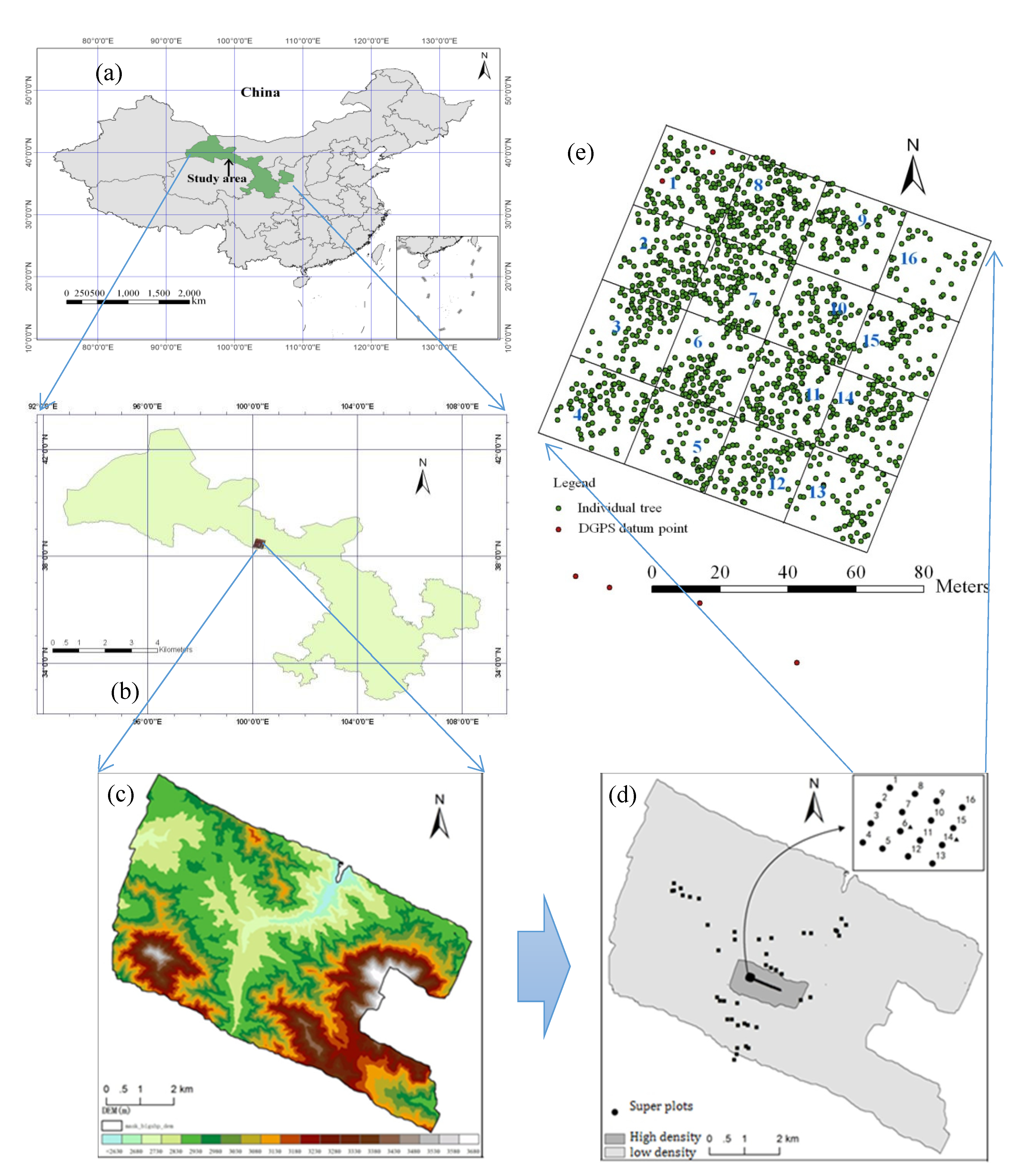
In this section, the iterative TIN algorithm was used to extract the ground points, and then four interpolation algorithms were used, and their accuracy was analyzed. In order to eliminate the influence of scanning angle, 27 LiDAR lines—each with a scanning degree of less than 10 degrees—were selected based on Terrasolid software, totaling 8,028,759 points, with an average density of 0.7 points/m². Iterative TIN algorithm assumes that the ground changes are smooth, and the large elevation changes in some areas are caused by buildings or vegetation [3]. Therefore, the ground points are screened by controlling the increment of slope. The extraction of ground points is to filter ground points based on a large grid and construct a sparse irregular triangular network. Then, a new triangular network is constructed with the initial ground points, and the iteration increment is calculated. The ground points are re-screened until the termination conditions of iteration or a certain number of iterations are met, the iteration is stopped, and the output is the expected result.

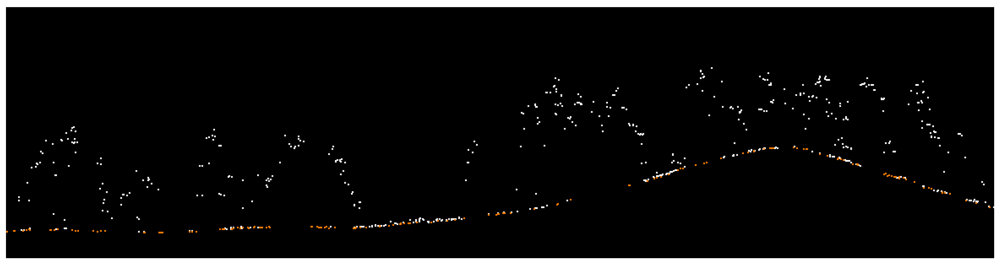
There are three types of parameters that need to be set in this algorithm: one is the initial mesh size, the other is the increment of iteration, and the third is the termination condition. According to the study area conditions, the parameters of the algorithm were set as follows: the initial mesh size was set to 60 m × 60 m; the termination conditions included terrain angle, iteration angle, and iteration distance, which were set to 88 degrees, 9 degrees, and 1.4 m, respectively; and the classification option was to stop iteration when the distance became less than 5 m. After calculation, 1,996,001 ground points were selected. One profile is shown in Figure 2. It showed that the algorithm did not detect all the ground points, but it was enough to construct high-precision DEM.

3.2. DEM Extraction Based on Interpolation Algorithms

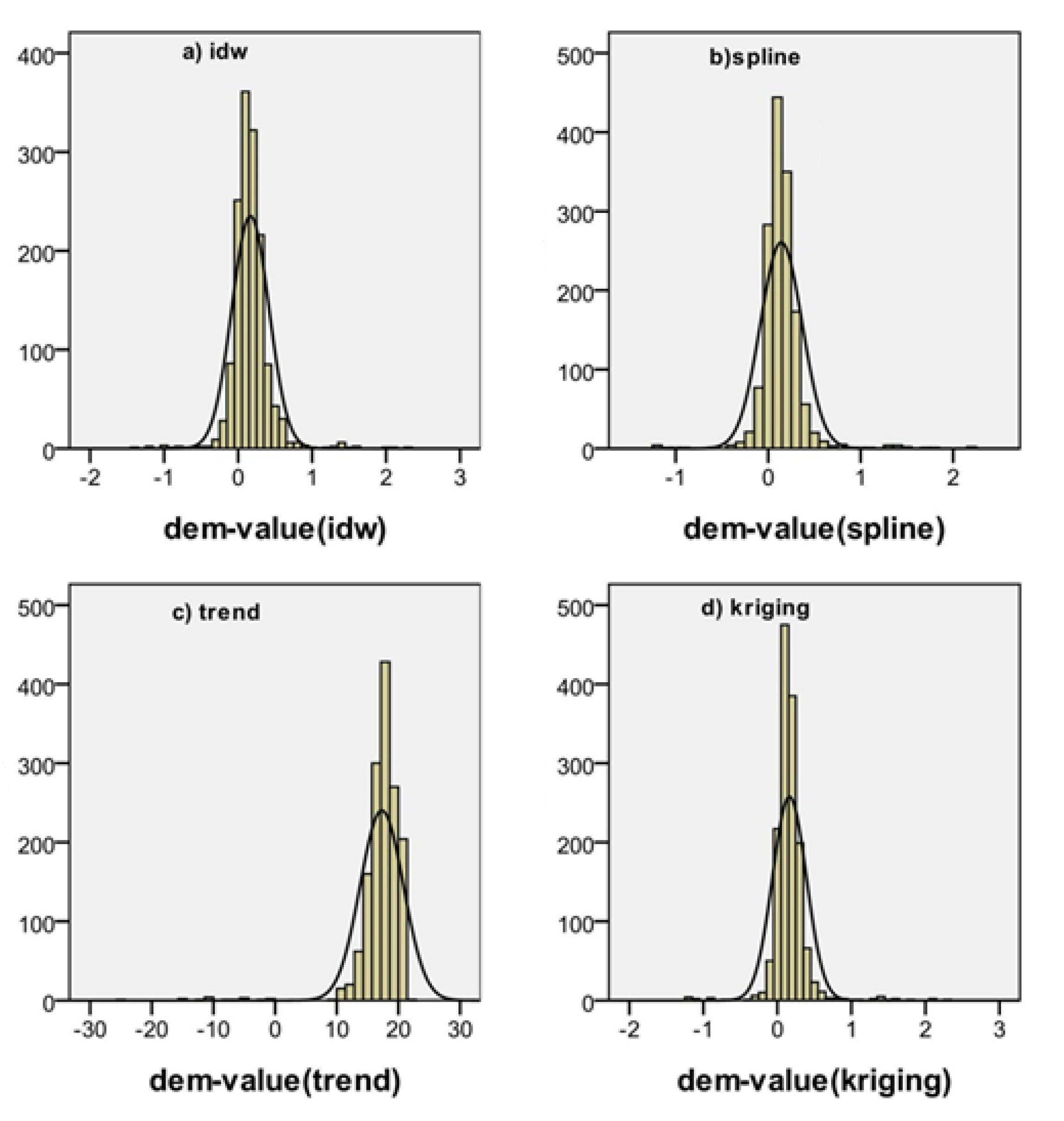
Based on the extracted ground points, DEM were generated, using an inverse distance weighted algorithm (IDW), a thin spline algorithm, a trend surface interpolation algorithm, and a Kriging algorithm.

(1) Inverse Distance Weighted Algorithm

The first law of geography states that the similarity between two objects decreases as their distance increases. Therefore, the closer to the target point, the higher the similarity with it, the higher the weight when estimating. Inverse Distance Weighted interpolation (IDW) is based on this model. The general equation of IDW is as follows:

$$z_0=\frac{{\displaystyle \sum _{i=1}^s{z}_i\frac{1}{d_i^k}}}{{\displaystyle \sum _{i=1}^s\frac{1}{d_i^k}}}$$

(1)

In the formula, Z0 is the estimated value of point 0; Zi is the Z value of point i; di is the distance between point i and point 0; s is the number of points involved in the estimation; and k is the power. Moreover, k denotes the relationship between similarity and distance of spatial objects. The larger the k value, the faster the similarity of things decays with increasing distance.

This method is simple, intuitive, and efficient. The interpolation effect of the algorithm is good when the distribution of known points is uniform. The interpolation results are between the maximum and minimum values of the interpolate data and are susceptible to extreme values.

(2) Thin Spline Algorithm

Thin spline function is based on known points, and a smooth interpolation curve is generated by using the polynomial fitting method. It has the feature that all points are on the surface, and the surface slope changes least. The approximate expression of the thin spline function is as follows:

$$Q(x,y)={\displaystyle \sum A_i}{d}_i^2\log d_i+a+bx+cy$$

(2)

Here, x and y indicate the abscissa and ordinate of the interpolation points; $d_i^2={(x-x_i)}^2+{(y-y_i)}^2$ represents the square of the distance from the known point i to the point to be interpolated; x_i and y_i are the abscissa and ordinate of control point i, respectively. Thin spline functions include two parts: ($a+bx+cy$) is a local trend function whose expression is similar to the first order linear trend surface; $d_i^2\log d_i$ is a basic function used to generate a surface with minimum curvature. The coefficients of $A_i$, a, b, and c are derived from the following linear equations.

$$\begin{array}{l}{\displaystyle \sum _{i=1}^n{A}_i{d}_i^2\log d_i+a+bx+cy}=f_i\\ \begin{array}{ccc}{\displaystyle \sum _{i=1}^n{A}_i}=0,& {\displaystyle \sum _{i=1}^n{A}_i{x}_i}=0,& {\displaystyle \sum _{i=1}^n{A}_i{y}_i}=0\end{array}\end{array}$$

(3)

In the formula, n is the number of control points, f_i is the known value of control point i, and the estimation of coefficients is a solution of an equation system consisting of n+3 equations.

Unlike IDW, the predicted values of thin spline function method are not limited to the maximum and minimum values of control points. This method has the advantages of easy operation and small computation [18]. However, it is difficult to estimate the error, and the interpolation effect is poor when the sampling points are scarce.

(3) Trend Surface Interpolation Algorithm

Trend surface analysis is based on the principle of regression analysis. Least squares method is used to fit a binary nonlinear function, to simulate the spatial distribution of geographical elements, and to show their change trend.

In field measurement, only discrete data can be obtained. Trend surface analysis builds polynomials based on these known points and estimates the values of other points. The first-order trend surface is expressed as follows:

$$z_{x,y}=b_0+b_{1}x+b_{2}y$$

(4)

In the formula, the attribute value Z is a function of coordinates x and y, and the coefficient bi is estimated by known points. The model uses the least square method to estimate bi, thus the fitting degree of the model can be measured.

Actually, the spatial distribution of geographic objects is more complex than the inclined surface generated by the first-order trend surface, such as the third-order surface containing mountains and valleys. This model is based on the following formula:

$$z_{x,y}=b_0+b_{1}x+b_{2}y+b_3{x}^2+b_{4}xy+b_5{y}^2+b_6{x}^3+b_7{x}^{2}y+b_{8}x{y}^2+b_9{y}^3$$

(5)

The first-order trend surface needs three coefficients, while the third-order trend surface needs to estimate 10 coefficients (bi), to predict the value of unmeasured points. The higher the order of the trend surface model is, the higher the accuracy is, and the larger the calculation amount is. Therefore, it is necessary to choose the appropriate model order according to the research complexity.

(4) Kriging Algorithm

Kriging is a geostatistical method for spatial interpolation. Compared with the previous three interpolation methods, Kriging can evaluate the prediction quality by estimating the prediction error. This study adopted the ordinary Kriging method. Assuming that there is no drift, the ordinary Kriging method only considers the spatially correlated factors and interpolates directly with the fitting semivariogram. The equation for estimating the Z value of a measurement point is as follows:

$$z_0={\displaystyle \sum _{i=1}^s{z}_x{w}_x}$$

(6)

In the formula, Z₀ is the value to be estimated; Z_x is the known value of x; w_x is the weight of x; and s is the number of sample points. The weight can be obtained by solving a set of simultaneous equations. For example, when estimating the value of an unknown point (0) from three known points (1, 2, 3), the three equations in (7) need to be combined.

$$\begin{array}{l}{W}_1\gamma (h_{11})+W_2\gamma (h_{12})+W_3\gamma (h_{13})+\lambda =\gamma (h_{10})\\ W_1\gamma (h_{21})+W_2\gamma (h_{22})+W_3\gamma (h_{23})+\lambda =\gamma (h_{20})\\ W_1\gamma (h_{31})+W_2\gamma (h_{32})+W_3\gamma (h_{33})+\lambda =\gamma (h_{i0})\\ W_1+W_2+W_3+0=1.0\end{array}$$

(7)

Here, γ(h_ij) is the semivariogram between known points i and j; γ(h_i0) is the semivariogram between the known point i and the unknown point; and λ is the introduced Lagrange coefficient to ensure the minimum estimation error.

After calculating the weight, Z0 can be estimated by Equation (8):

$$z_0=z_1{W}_1+z_2{W}_2+z_3{W}_3$$

(8)

The abovementioned equations indicate that Kriging method considers not only the relationship between estimated points and known points, but also the semivariogram between known points when calculating weights. Compared with other local fitting methods, Kriging calculates the variation of each estimated point, and the interpolation accuracy is higher.

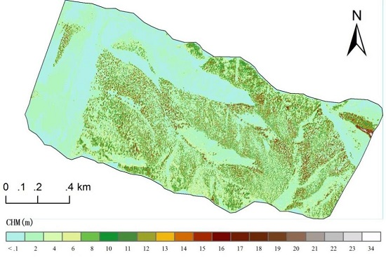
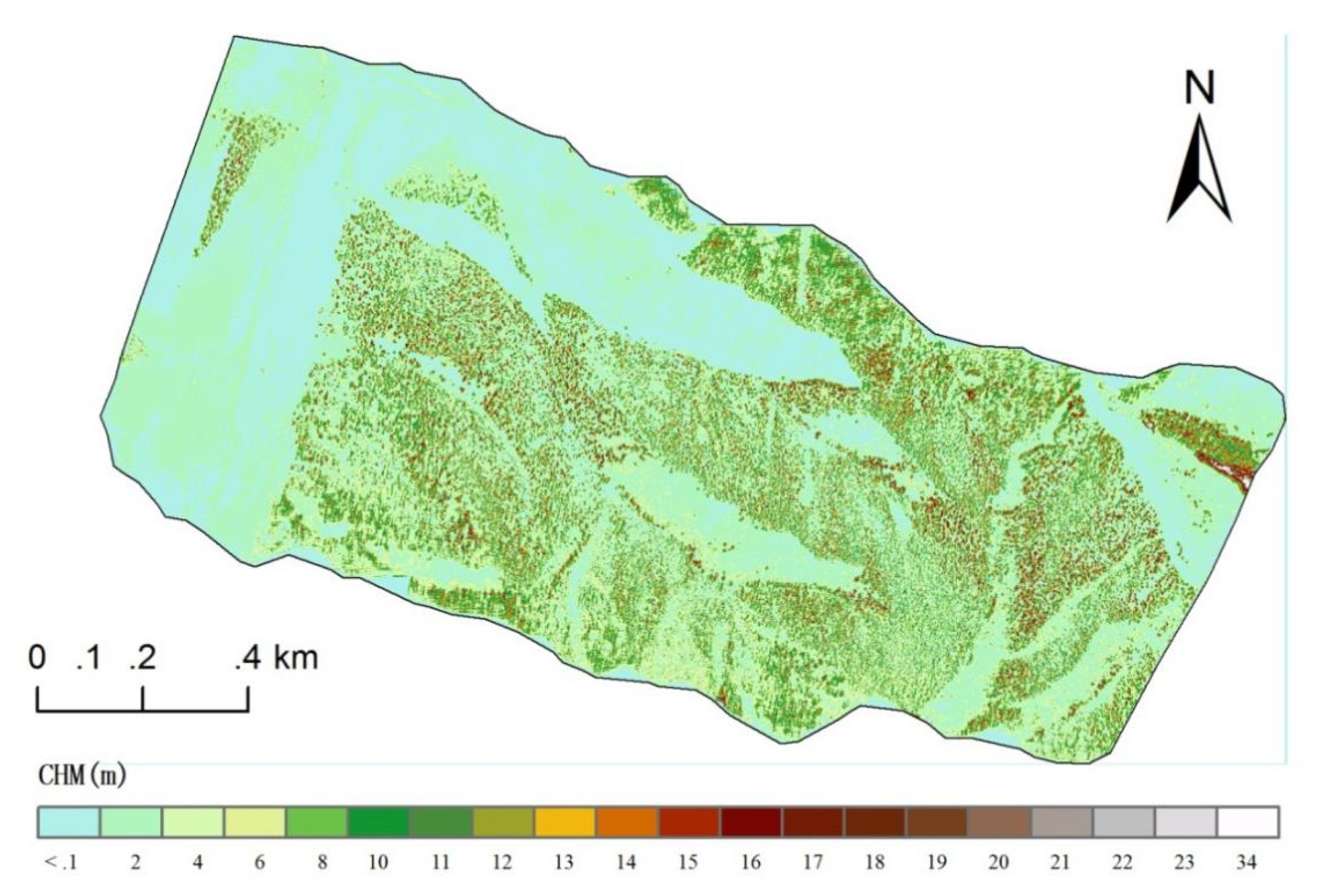
The DEM was acquired by the interpolation method. The height of the point cloud was assigned to the DSM and the CHM was acquired.

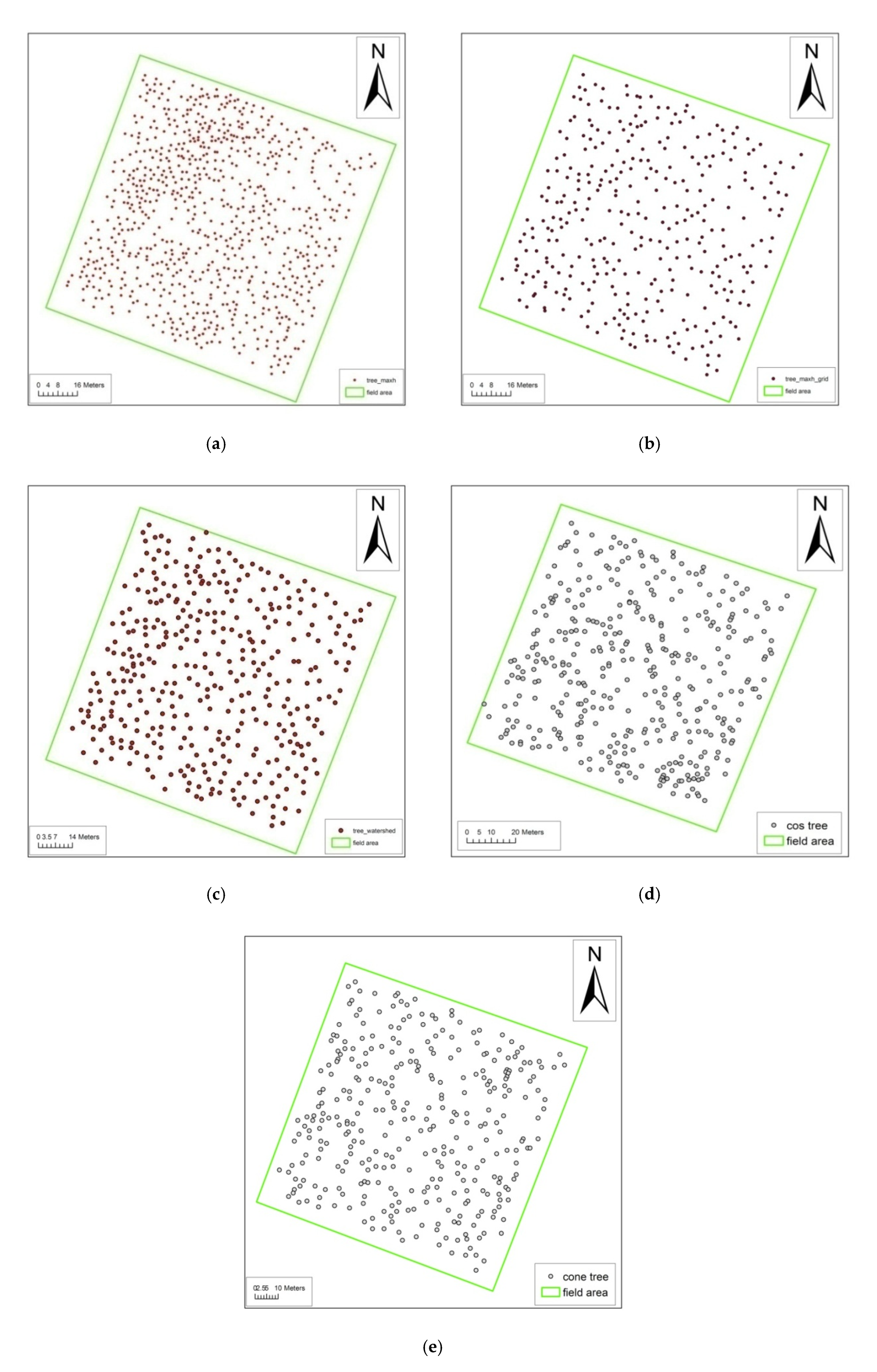
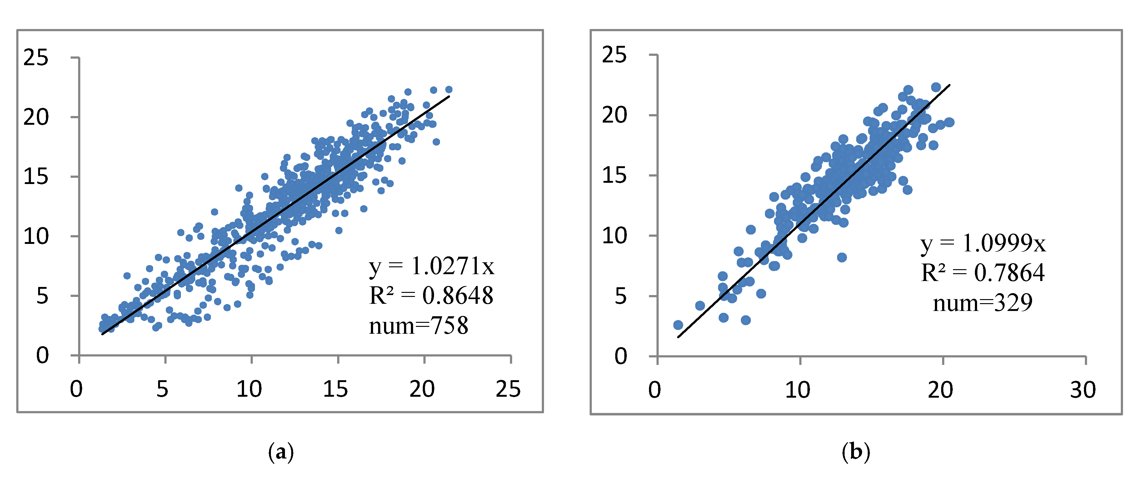
3.3. Individual Tree Parameter Inversion Algorithm

(1) Local Maximum Algorithms Based on Point Clouds

Local maximum algorithms based on point clouds searches the maximum value in a certain window size as the treetop position. It needs to set the window size according to the distribution and structure of the tree crown. For the same forest stand with uniform crown size, a fixed window size can be used. When the crown size varies greatly, the fixed search window can easily produce pseudo treetop or miss crown vertices. A feasible alternative is to determine the search window size according to the relationship between tree height and crown width [30]. For the forest area with the same tree species of Picea crassifolia, there is a linear relationship between tree height and crown width [18]:

$$Y=0.202X+1.355$$

(9)

Here, X denotes tree height, and Y denotes crown width. The parameters of the equation were determined by linear regression of measured tree height and crown width in the surveyed plots.

Firstly, the LiDAR point cloud data in xyz format was transformed into shp format, and then the elevation value of DEM was extracted and assigned to each point, and the difference between the height of point cloud and DEM was calculated, so that the distance between each point and ground was obtained. Based on this, the Thiessen polygons and TIN were constructed, and the volume was calculated by taking the height of the interior point of the Thiessen polygon as the base. If the volume was 0, it indicated that the point was the highest and was reserved as an individual treetop [22]. Then, the points with height less than 1.3 m were removed. Finally, using the relationship between tree height and crown width (Equation (9)), the pseudo-single-tree points which did not satisfy the conditions were gradually eliminated.

(2) Local Maximum Algorithms Based on CHM

In order to eliminate the noise in CHM, a 3 × 3 pixel mean filtering operation was performed on CHM, and then the local maximum of 3 × 3 pixel windows was searched as the candidate point of the treetop [6,18]. Finally, the theoretical crown width was calculated according to the tree height and Equation (9) of the candidate points. When the distance between the two candidate points was less than half of the theoretical crown width, the points with a smaller tree height were removed until the distance among all the points was greater than half of the theoretical crown width.

(3) Watershed Algorithm

A watershed is a mountain or plateau that separates two adjacent basins from which the river flows in two opposite directions. The watershed algorithm is the watershed transform based on the overflow model. It regards the gray value of the image as the elevation, and the water immerses the surface from the water-accumulation point, and gradually submerges the image at the same speed. When the rising water level from different minimum values meets, a dam is constructed to block it. Until only the top of the dam is above the water surface, the procedure is terminated and the segmentation is completed.

Taking two pixels as radius, the mean filtering of CHM (with a spatial resolution of 0.5 m) was carried out, and the inverse was obtained. In this way, a large number of small gullies were obtained. On this basis, basin function embedded in ArcGIS tool was used to extract watershed. The highest value of each basin was taken as the height of an individual tree, and the location was taken as the position of an individual tree.

(4) Template-Matching Algorithm

Template-matching algorithm is a method to find objects similar to the template from the original images according to the distance or correlation. This technology is often used in image registration, interferometric SAR, and other remote-sensing data processing. The correlation coefficient can be used as an index to measure the matching degree of the template and graph (Equation (10)).

$$r=\frac{{\displaystyle \sum (x_i-\overline{x})(y_i-\overline{y})}}{\sqrt{{\displaystyle \sum {(x_i-\overline{x})}^2}}\sqrt{{\displaystyle \sum {(y_i-\overline{y})}^2}}}$$

(10)

Here, x_i represents the gray value of the template, and y_i represents the gray value of the detected image. When r = 1, it indicates that the current position is positively correlated with the template and the matching is successful; when r = 0, they are completely unrelated, or not the search target; if r = −1, this means that they are negatively correlated and need to be re-detected by rotation or other operations.

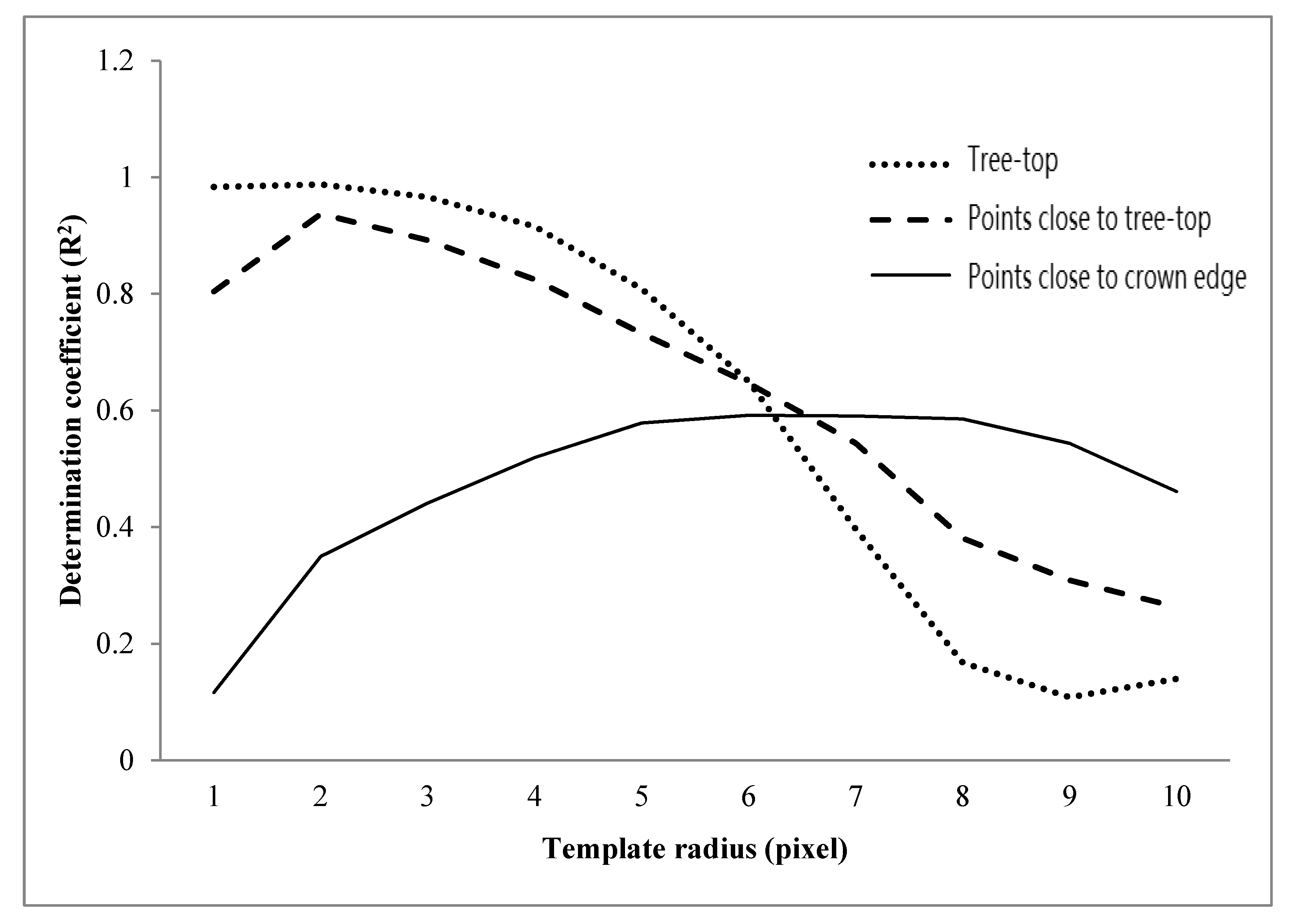
In this study, the mean filtering of 3 × 3 was performed, and then the maximum value in the neighborhood of 3 × 3 was extracted. With this point as the center, the correlation coefficients were obtained by using two-dimensional cosine function and conic function whose diameter was 3, 5, 7, 9, 11, 13, 15, 17, and 19 pixels and height was equal to the height of the treetop. Finally, the maximum value of correlation coefficient greater than 0.8 was retained as the single tree position, and the diameter of the maximum deceleration rate of correlation coefficient was used as the crown width.

As shown in Figure 3, when the matching point is located at the top of the tree, the matching point extends gradually to the ground and the surrounding crown, and the determination coefficient of the crown and the model decreases gradually. When the matching points are located in the canopy around the treetop, with the increase in the radius, the matching points gradually extend to the ground and the surrounding canopy, and the correlation coefficient between the canopy and the model decreases first, then increases, and finally decreases. This rule can be used to extract the crown width of individual trees.

4. Results

4.1. DEM

Based on the extracted ground points, DEMs were generated by using an IDW algorithm, a thin spline algorithm, a trend surface interpolation algorithm, and a Kriging algorithm, and the accuracy of these interpolation algorithms was compared. The parameters used for the interpolation are shown in

Table 3. The parameters used for the interpolation methods.

Parameter Type	Parameter Name	Setting
Common parameters	Input point features	Input file, las.shp
	Z value field	Shape.Z
	Output raster	Output file
	Output cell size	0.5
IDW algorithm	Power	2
Trend algorithm	Polynomial order	2
	Type of regression	linear
Spline algorithm	Weight	0.1
	Spline type	tension
Kriging algorithm	Kriging method	Universal
	Semivariogram model	Linear with linear drift

.

Considering the large number and high density of ground points, the verification could be conducted by using field-measured data, and the results are shown in

Table 4. The statistical table of the errors.

Statistical Data	IDW	Spline	Trend	Kriging
Average	0.17	0.14	17.30	0.16
Mean Standard Error	0.00651	0.00588	0.09114	0.00595
Standard Deviation	0.25037	0.22592	3.50260	0.22858
Variance	0.063	0.051	12.268	0.052
Skewness	1.409	1.953	−5.509	1.962
Kurtosis	15.232	22.294	46.086	24.610
Range	3.70	3.40	47.20	3.50
Minimum	−1.40	−1.20	−25.40	−1.20
Maximum	2.30	2.20	21.80	2.30

and Figure 4. The results indicated that the trend surface interpolation results were on the high side, and the error was the largest; the thin spline interpolation algorithm has the lowest error, followed by the Kriging algorithm. As can be seen from Table 4, except for trend surface interpolation, there was little difference among the other three algorithms. To be precise, the accuracy of the thin spline algorithm was slightly higher. Therefore, a thin spline interpolation algorithm was used to extract DEM.

4.2. CHM

Based on the ground points, the thin spline algorithm was used to generate DEM. The height of the point cloud of LiDAR was assigned to the DSM directly. The DSM was then subtracted from the DEM to obtain CHM, as shown in Figure 5.

4.3. Individual Tree Position, Tree Height, and Crown Width

In this study, the local maximum method (point cloud based and CHM based), watershed algorithm and template-matching algorithm (cosine template and cone template) were used, respectively, to extract individual tree parameters, and the extraction accuracies of the individual tree position, tree height, and crown width were compared and analyzed. The local maximum algorithm (Max_CHM), watershed algorithm, and template-matching algorithm were all based on CHM, and the local maximum algorithm based on point cloud (Max_H) used high-density point cloud as the original data for inversion. The results of these algorithms were validated, using the measured individual tree information in the super plots, and the accuracy was analyzed from three perspectives: the number of detected individual tree, tree-height error, and crown-width error.

Figure 6 showed the matching results of extracted and the nearest measured individual trees. If there were multiple points matching with one extracted tree, the points with similar height were selected. Among them, (a) the number of individual trees obtained by the Max_H algorithm was 1119, and there were 758 matching results with the measured ones; (b) the number from Max_CHM algorithm was 437, and only 329 matched with the measured trees; (c) the watershed algorithm extracted 544 trees, and 372 matched; (d) the cosine-template-matching algorithm extracted 676, and only 370 matched; and (e) the number from cone-template-matching algorithm was 658, and the matching result was only 330.

To further compare and analyze the accuracy of all the algorithms, the number of trees, average tree height, and crown width were calculated in 16 sample plots.

Table 5. The counts of tree extracted by these five algorithms in 16 super plots.

Plot No.	Number of Trees	Max_H	Max_CHM	Watershed	Cosine Template Matching	Cone Template Matching
1	98	47	20	24	18	18
2	113	63	24	27	25	26
3	77	49	25	30	29	29
4	80	45	24	24	22	20
5	69	36	18	20	20	17
6	90	43	19	19	21	17
7	120	58	25	28	28	22
8	153	80	24	27	20	19
9	86	44	20	23	21	21
10	99	44	20	23	21	15
11	110	45	17	19	21	17
12	92	51	24	26	28	20
13	61	38	21	23	36	24
14	93	47	20	25	23	23
15	76	41	13	16	19	16
16	36	27	15	18	18	26

and Figure 7 indicated that the lower the height of the trees, the fewer actual field trees that can be extracted. For example, in sample plot 8, the extracted tree number is only 1/7 of the field number; in sample plots 1, 10, and 11, there were about 100 trees with an average tree height of 8.2 m, and the extracted tree based on CHM was only 1/5 of the field number. The higher the trees were, the more trees were extracted; for example, in sample plots 3 and 4, there were about 80 trees with an average tree height of 11.5 m, the number of individual trees extracted based on CHM reached 1/4 of the field number.

Table 6. The statistics of the tree extracted by watershed algorithm in 16 super plots.

Plot No.	Number of Trees	Measured Tree Height (m)	Extracted Tree Height (m)	Measured Crown Width (m)	Extracted Crown Width (m)
1	24	13.35	13.98	4.45	5.47
2	27	14.45	13.98	4.50	5.32
3	30	15.66	14.90	4.46	4.96
4	24	15.40	15.38	4.20	5.13
5	20	15.65	15.54	5.09	5.93
6	19	15.12	15.24	4.36	5.42
7	28	13.73	13.70	4.16	5.48
8	27	10.05	9.92	3.37	5.09
9	23	14.32	13.63	4.39	6.33
10	23	13.64	12.99	4.22	5.45
11	19	15.61	15.56	5.38	6.43
12	26	16.13	16.30	4.56	5.17
13	23	17.12	17.43	5.59	5.87
14	25	15.79	15.39	4.60	5.56
15	16	14.99	15.56	5.46	6.73
16	18	15.69	14.53	5.19	6.49
		Average Error	0.39		1.05
		RMSE	0.51		1.13

showed that the individual tree height extracted by watershed algorithm was close to the measured value, and the accuracy was high (RMSE = 0.51). It should be noted that when there were too many trees in the forest, the LiDAR signal could not penetrate, even if a few signals reached the treetops, the watershed algorithm cannot capture these features. Some extracted tree height was higher than the measured value, which was mainly due to three causes: (1) the canopy closure was larger and the measurement accuracy was poor; (2) the positioning error of point cloud lead to the error that adjacent canopy points of higher trees was regarded as the treetop; and (3) the field survey located individual trees by the root of the tree, while the individual trees extracted from the LiDAR point cloud located tree position by the tree top. Due to the influence of wind and slope, the top and root of trees were not always in the same vertical line, which brought positioning errors.

In terms of crown width extraction, the watershed algorithm generally produced higher values than the measured ones, and the error was about 1.0 m (RMSE = 1.13). This was because watershed algorithm divided the whole region and took the area of each basin as the crown coverage. Actually, there were some forest gaps which were not covered by the crown also included in the watershed calculation output. This leads to the overestimated crown width. The accuracy of crown width extraction, using the watershed algorithm, was lower than that of tree-height extraction.

The results of the template-matching algorithm are shown in

Table 7. The statistics of the tree extracted by template-matching algorithm (cosine) in 16 super plots.

Plot No.	Number of Trees	Measured Tree Height (m)	Extracted Tree Height (m)	Measured Crown Width (m)	Extracted Crown Width (m)
1	18	11.66	8.57	4.26	4.50
2	25	12.59	8.87	4.42	3.30
3	29	13.4	10.33	4.57	4.02
4	22	13.49	10.22	4.01	4.05
5	20	13.54	11.08	4.51	5.00
6	21	10.8	9.48	3.60	4.88
7	28	13.36	9.83	4.22	4.29
8	20	7.38	5.40	2.82	3.50
9	21	13.13	8.01	4.48	4.31
10	21	11.49	9.37	3.78	4.93
11	21	13.22	8.99	4.74	4.50
12	28	13.13	10.12	3.97	3.54
13	36	14.88	12.66	4.94	4.86
14	23	14.64	10.88	4.32	5.15
15	19	12	8.71	4.66	4.82
16	18	14.02	9.64	4.69	4.94
		Average Error	3.16		0.48
		RMSE	3.30		0.63

and

Table 8. The statistics of the tree extracted by template-matching algorithm (cone) in 16 super plots.

Plot No.	Number of Trees	Measured Tree Height (m)	Extracted Tree Height (m)	Measured Crown Width (m)	Extracted Crown Width (m)
1	18	12.2	8.6	4.5	5.1
2	26	12.4	8.5	4.4	4.5
3	29	13.5	9.7	4.5	4.5
4	20	12.9	9.7	3.8	4.6
5	17	12.7	11.2	4.2	4.9
6	17	11.2	9.3	3.8	4.8
7	22	13.0	9.4	4.1	5.0
8	19	7.7	5.2	2.9	3.8
9	21	13.7	8.3	4.5	5.0
10	15	11.3	9.6	3.8	4.6
11	17	12.4	9.0	4.5	5.0
12	20	13.6	10.4	4.1	4.2
13	24	15.6	12.6	5.0	4.7
14	23	15.0	10.8	4.4	5.7
15	16	11.5	8.7	4.5	4.5
16	26	13.4	9.6	4.8	5.3
		Average Error	3.22		0.56
		RMSE	3.36		0.67

. Comparisons indicated that the extraction performance of cosine template was slightly better than that of cone template-matching algorithm (Table 8). The tree height extracted by the two template-matching algorithms was significantly lower, and the error was larger (RMSE = 3.30 for cosine and 3.36 for cone), but the accuracy of crown width extraction was higher than that of the watershed algorithm (RMSE = 0.63 for cosine and 0.67 for cone).

In summary, the algorithms of Max_H and Max_CHM can effectively extract the treetop and determine the location of individual trees. The watershed algorithm can accurately extract individual tree height and determine the maximum edge of the tree crown; the template-matching algorithm can be used to extract accurate individual tree crown width, in which the cosine template performed slightly better than the cone template.

5. Discussion

In this study, airborne LiDAR-based individual tree parameter inversion algorithms were systematically studied, and the understory DEM interpolation algorithms and individual tree parameter extraction algorithms were compared and analyzed. Among them, aiming at DEM interpolation algorithm, the thin spline interpolation algorithm achieved the highest accuracy, followed by the Kriging interpolation algorithm, and the trend surface interpolation algorithm had the lowest accuracy. According to the analysis of individual tree parameter inversion results, it was found that the local maximum algorithm can effectively extract the treetop, which can be used to determine the position of individual trees, but can also easily extract data for too many treetops; the watershed algorithm can effectively estimate the height and maximum crown width of individual tree, but it was necessary to remove the impact of some non-canopy areas (e.g., forest gaps). The template-matching algorithm had the lowest accuracy in tree-height inversion, but it could be used to extract crown width accurately, combined with watershed algorithm. Overall, the detection and delineation accuracy of individual tree parameters in this study is generally consistent with the results from previous studies, especially for those with the same tree species [3,10,11,13,17,34,35]. However, there are some exceptions. These results are partly consistent with those reported in the study of Edson and Wing [30] for the tree position. They pointed out that the Fusion software (using the local maximum algorithm of Max_H) had the highest accuracy in tree-position determination, and the watershed algorithm had the lowest accuracy. However, they also reported that the TreevaW software (using the local maximum algorithm of Max_CHM) had the highest accuracy in tree-height extraction, and also that the watershed algorithm gave the worst performance for the tree height. This part is not consistent with the result of our study. Through further analysis and comparison, we find that the reason lies in the difference of tree density between the two study areas, which leads to a difference of tree gap and then affects the accuracy of tree-height extraction based on watershed algorithm.

When detecting the position of individual trees, a Max_H algorithm is simple in principle and easy to implement, and thus shows itself to be the best algorithm to preliminarily determine the treetop positions. In fact, there were totally 6013 candidate points extracted by Max_H algorithm in this study, and 2437 points were reserved after removing the points whose height was less than 1.3 m; 1119 were kept after screening, and 758 effective individual trees were matched with the measured trees. Therefore, when removing those extracted points with the same matched individual trees, different levels of human impacts are revealed. The watershed algorithm can determine the canopy edge on this basis. This algorithm does not make full use of the information of canopy surface and is greatly influenced by the search window. Different from the watershed algorithm, the Max_CHM algorithm produced fewer candidate points, but more matched with field measured individual trees; therefore, there is less human disturbance in matching factors. As the tree density in the sample plots is 1.5 trees/m², which is relatively high, and the structure is complex, the template-matching algorithm cannot effectively identify individual trees from the crown of multi-tree aggregation [23]; thus, the errors are the largest among these algorithms when detecting individual tree positions.

In this study, the tree-position error is another effective indicator for the accuracy verification of the individual tree extraction results. However, considering that the top and root of lots of trees in the plots are not on the same vertical line due to the influence of wind and slope, it is difficult to eliminate this type of error; therefore, the tree-position error has not been taken as an accuracy-assessment indicator. It should be considered in future research, especially in field forest measurements.

The reasons why the number of individual trees detected in this study is less than the field measured value are as follows: (1) the forest density is high, and the adjacent trees are covered with each other; (2) the template features are simple, and the detection capacity of the forest distribution with multi-tree aggregation method remains to be improved. Compared with the extraction algorithm based on point clouds, the accuracy of the algorithm based on CHM is poor. In addition, for extremely dense forests, it is difficult to extract individual trees effectively due to the limitation of laser pulse’s penetration ability. It is consistent with the conclusions of some previous studies [4,10,20]. In the study of Cao et al. [4,10], the tree height was estimated with high accuracy, while there was a large error in extracting the crown widths, due to the impact of adjacent trees.

This study provides an essential reference for the algorithm selection for forest individual tree parameter inversion based on airborne LiDAR data. It also assists with accurate forest monitoring and management applications. When the airborne LiDAR data is used for the forest monitoring, the methodology should be selected according to the monitoring purpose. If it is only the number of trees needed, the local maximum algorithm is the optimal choice, and, additionally, the CHM is not necessary under this circumstance [6,22]; if the tree height and crown width of individual trees are the delineation objectives, then we should combine the watershed and template-matching algorithms, to extract the required structural parameters with high precision. During such a process, CHM is mandatory. The detection and extraction accuracy is determined by both the algorithm itself and the site conditions.

6. Conclusions

In this study, through the comparative analysis of individual tree parameter extraction algorithms, it was found that the accuracy of individual tree position detection and tree-height extraction based on point clouds is much higher than those based on CHM, but the crown width cannot be obtained from point clouds directly. Among the three examined algorithms based on CHM, the local maximum algorithm of Max_CHM can be used to extract the potential treetop position effectively; the watershed algorithm can extract tree height more effectively and find the maximum distribution range of crown width, which provides the maximum matching range for template-matching algorithm and reduces its time complexity; finally, the template-matching algorithm can accurately extract the crown width of individual trees. Combining the three algorithms cannot only improve the accuracy of individual tree parameter extraction, but also improve the efficiency in forest monitoring and management applications.

References

1. Hense, S.; Lucht, W.; Schmullius, C.; Barnsley, M.; Dubayah, R.; Knorr, D.; Neumann, K.; Riedel, T.; Schröter, K. Global biomass mapping for an improved understanding of the CO2 balance—The Earth observation mission Carbon-3D. Remote Sens. Environ. 2005, 94, 94–104. [Google Scholar]
2. Chen, W.; Jiang, H.Z.; Moriya, K.; Sakai, T.; Cao, C.X. Monitoring of post-fire forest regeneration under different restoration treatments based on ALOS/PALSAR data. New Forest. 2018, 49, 105–121. [Google Scholar] [CrossRef]
3. Bao, Y.F.; Cao, C.X.; Zhang, H.; Chen, E.X.; He, Q.S.; Huang, H.B.; Li, Z.; Li, X.; Gong, P. Synchronous estimation of DTM and fractional vegetation cover in forested area from airborne LiDAR height and intensity data. Sci. China Ser. E 2008, 51, 176–187. [Google Scholar] [CrossRef]
4. Cao, C.X.; Bao, Y.F.; Xu, M.; Chen, W.; Zhang, H.; He, Q.S.; Li, Z.Y.; Guo, H.D.; Li, J.H.; Li, X.W.; et al. Retrieval of forest canopy attributes based on Geometric-Optical model using airborne LiDAR and optical remote sensing data. Int. J. Remote Sens. 2012, 33, 692–709. [Google Scholar] [CrossRef]
5. Chen, W.; Zhao, J.; Cao, C.X.; Tian, H.J. Shrub biomass estimation in semi-arid sandland ecosystem based on remote sensing technology. Glob. Ecol. Conserv. 2018, 16, e00479. [Google Scholar] [CrossRef]
6. Huang, H.B. The Forest Structural Parameter Extraction using LiDAR. Ph.D. Thesis, Institute of Remote Sensing Applications, Chinese Academy of Sciences, Beijing, China, 2008. [Google Scholar]
7. Hollaus, M.; Wagner, W.; Eberhoefer, C.; Karel, W. Accuracy of large–scale canopy heights derived from LiDAR data under operational constraints in a complex alpine environment. ISPRS J. Photogramm. 2006, 60, 323–338. [Google Scholar] [CrossRef]
8. Dong, L.X.; Tang, S.H.; Min, M.; Veroustraete, F.; Cheng, J. Aboveground forest biomass based on OLSR and an ANN model integrating LiDAR and optical data in a mountainous region of China. Int. J. Remote Sens. 2019, 40, 6059–6083. [Google Scholar] [CrossRef]
9. Hopkinson, C.; Chasmer, L.; Hall, R.J. The uncertainty in conifer plantation growth prediction from multi-temporal lidar datasets. Remote Sens. Environ. 2008, 112, 1168–1180. [Google Scholar] [CrossRef]
10. Cao, C.X.; Bao, Y.F.; Chen, W.; Dang, Y.F.; Li, L.; Tian, R.; Li, G.H. Extraction of forest structural parameters based on the intensity information of high-density airborne LiDAR. J Appl. Remote Sens. 2012, 6, 063533. [Google Scholar]
11. Wu, X.; Shen, X.; Cao, L.; Wang, G.; Cao, F. Assessment of Individual Tree Detection and Canopy Cover Estimation using Unmanned Aerial Vehicle based Light Detection and Ranging (UAV-LiDAR) Data in Planted Forests. Remote Sens. 2019, 11, 908. [Google Scholar] [CrossRef] [Green Version]
12. Holmgren, J.; Persson, Å. Identifying species of individual trees using airborne laser scanning. Remote Sens. Environ. 2004, 90, 415–423. [Google Scholar] [CrossRef]
13. Chen, Q.; Baldocchi, D.; Gong, P. Isolating Individual Trees on Savanna woodland using small footprint LIDAR data. Photogramm. Eng. Rem. S. 2006, 72, 923–932. [Google Scholar] [CrossRef] [Green Version]
14. Kathuria, A.; Turner, R.; Stone, C.; Duque-Lazo, J.; West, R. Development of an automated individual tree detection model using point cloud LiDAR data for accurate tree counts in a Pinus radiata plantation. Aust. For. 2016, 79, 126–136. [Google Scholar] [CrossRef]
15. Yin, D.M.; Wang, L. Individual mangrove tree measurement using UAV-based LiDAR data: Possibilities and challenges. Remote Sens. Environ. 2019, 223, 34–49. [Google Scholar] [CrossRef]
16. Suarez, J.C.; Ontiveros, C.; Smith, S.; Snape, S. Use of airborne LiDAR and aerial photography in the estimation of individual tree heights in forestry. Comput. Geosci.-UK 2005, 31, 253–262. [Google Scholar] [CrossRef]
17. Andersen, H.E.; Reutebuch, S.E.; McGaughey, R.J. A rigorous assessment of tree height measurements obtained using airborne LiDAR and conventional field methods. Can. J. Remote Sens. 2006, 32, 355–366. [Google Scholar] [CrossRef]
18. Bao, Y.F. Study on Methods of forest Parameters Extraction from Multi-Source Remote Sensing Data. Ph.D. Thesis, Institute of Remote Sensing Applications of Chinese Academy Sciences, Beijing, China, 2009. [Google Scholar]
19. Liu, Q.W. Study on the Estimation Method of Forest Parameters Using Airborne LIDAR. Ph.D. Thesis, Chinese Academy of Forestry, Beijing, China, 2009. [Google Scholar]
20. Burt, A.; Disney, M.; Calders, K. Extracting individual trees from lidar point clouds using treeseg. Methods Ecol. Evol. 2019, 10, 438–445. [Google Scholar] [CrossRef] [Green Version]
21. Popescu, S.C.; Wynne, R.H.; Nelson, R.F. Measuring individual tree crown diameter with lidar and assessing its influence on estimating forest volume and biomass. Can. J. Remote Sens. 2003, 29, 564–577. [Google Scholar] [CrossRef]
22. Takahashi, T.; Yamamoto, K.; Senda, Y.; Tsuzuku, M. Estimating individual tree heights of sugi (Cryptomeria japonica D. Don) plantations in mountainous areas using small-footprint airborne LiDAR. J. Forest Res.-JPN 2005, 10, 135–142. [Google Scholar] [CrossRef]
23. Kwak, D.A.; Lee, W.K.; Lee, J.H.; Biging, G.S.; Gong, P. Detection of individual trees and estimation of tree height using LiDAR data. J. For. Res.-JPN 2007, 12, 425–434. [Google Scholar] [CrossRef]
24. Goodwin, N.R.; Coops, N.C.; Culvenor, D.S. Assessment of forest structure with airborne LiDAR and the effects of platform altitude. Remote Sens. Environ. 2006, 103, 140–152. [Google Scholar] [CrossRef]
25. Dalponte, M.; Frizzera, L.; Gianelle, D. Individual tree crown delineation and tree species classification with hyperspectral and LiDAR data. Peerj 2019, 6, e6227. [Google Scholar] [CrossRef] [PubMed]
26. Li, W.; Guo, Q.; Jakubowski, M.K.; Kelly, M. A New Method for Segmenting Individual Trees from the Lidar Point Cloud. Photogramm. Eng. Remote Sens. 2012, 78, 75–84. [Google Scholar] [CrossRef] [Green Version]
27. Yan, Z.J.; Liu, R.F.; Cheng, L. A Concave Hull Methodology for Calculating the Crown Volume of Individual Trees Based on Vehicle-Borne LiDAR Data. Remote Sens. 2019, 11, 623. [Google Scholar] [CrossRef] [Green Version]
28. Morsdorf, F.; Koetz, B.; Meier, E.; Itten, K.I.; Allgöwer, B. Estimation of LAI and fractional cover from small footprint airborne laser scanning data based on gap fraction. Remote Sens. Environ. 2006, 104, 50–61. [Google Scholar] [CrossRef]
29. Lee, H.; Slatton, K.C.; Roth, B.E.; Cropper, W.P. Adaptive clustering of airborne LiDAR data to segment individual tree crowns in managed pine forests. Int. J. Remote Sens. 2010, 31, 117–139. [Google Scholar] [CrossRef]
30. Edson, C.; Wing, M.G. Airborne Light Detection and Ranging (LiDAR) for Individual Tree Stem Location, Height, and Biomass Measurements. Remote Sens. 2011, 3, 2494–2528. [Google Scholar] [CrossRef] [Green Version]
31. Chang, A.J.; Eo, Y.D.; Kim, Y.M.; Kim, Y. Identification of individual tree crowns from LiDAR data using a circle fitting algorithm with local maxima and minima filtering. Remote Sens. Lett. 2013, 4, 29–37. [Google Scholar] [CrossRef]
32. Tang, S.J.; Dong, P.L.; Buckles, B.P. Three-dimensional surface reconstruction of tree canopy from lidar point clouds using a region-based level set method. Int. J. Remote Sens. 2013, 34, 1373–1385. [Google Scholar] [CrossRef]
33. Dai, W.X.; Yang, B.S.; Dong, Z.; Shaker, A. A new method for 3D individual tree extraction using multispectral airborne LiDAR point clouds. ISPRS J. Photogramm. 2018, 144, 400–411. [Google Scholar] [CrossRef]
34. Brandtberg, T.; Warner, T.A.; Landenberger, R.E.; McGraw, J.B. Detection and analysis of individual leaf-off tree crowns in small footprint, high sampling density lidar data from the eastern deciduous forest in North America. Remote Sens. Environ. 2003, 85, 290–303. [Google Scholar] [CrossRef]
35. Swinfield, T.; Lindsell, J.A.; Williams, J.V.; Harrison, R.D.; Agustiono; Habibi; Gemita, E.; Schönlieb, C.B.; Coomes, D.A. Accurate Measurement of Tropical Forest Canopy Heights and Aboveground Carbon Using Structure From Motion. Remote Sens. 2019, 11, 928. [Google Scholar] [CrossRef] [Green Version]
Figure 1. Location of the study area and investigated plots: (a,b) the study area of Dayekou forestry site in Gansu, China; (c) Digital Elevation Model (DEM) map; (d) distribution of LiDAR points and field data; (e) individual trees distribution in the field measurements, the numbers on this figure are the super plot numbers.
Remotesensing 12 00571 g001
Figure 2. The profile of ground point separation results (orange ones indicate the ground points, and white ones are the non-ground point.).
Remotesensing 12 00571 g002
Figure 3. The determination coefficient trend variance of correlation with the treetop and crown for different radius with cosine function.
Remotesensing 12 00571 g003
Figure 4. The error histogram of the four interpolation algorithms: (a) inverse distance weighted (IDW), (b) thin spline, (c) trend surface, and (d) Kriging algorithms (X-axis = the difference between the measured and interpolated elevation; Y-axis = frequency).
Remotesensing 12 00571 g004
Figure 5. The canopy height model (CHM) of the study area.
Remotesensing 12 00571 g005
Figure 6. The distribution of the individual trees extracted by five different algorithms: (a) Max_H, (b) Max_CHM, (c) watershed, (d) cosine-template-matching, and (e) cone-template-matching algorithms.
Remotesensing 12 00571 g006
Figure 7. The scatter plot of the measured and extracted tree heights by (a) Max_H, (b) Max_CHM, (c) watershed, (d) cosine-template-matching, and (e) cone-template-matching algorithms (X-axis is measured tree height; Y-axis is extracted tree height).
Remotesensing 12 00571 g007aRemotesensing 12 00571 g007b