1. Introduction
The accuracy of wave regime assessment and forecasting is one of the greatest challenges for the development and safety of marine activities. Unfortunately, traditional in situ wave gauges, such as buoys, the most extended one, are single-point measuring devices which also have other limitations, such as the difficulty of making an accurate mooring installation to avoid interference in wave measurements and the risk of suffering accidents or vandalism on the water surface. Together with the difficulty of doing maintenance and repairs during some seasons due to harsh weather conditions, this all usually leads to many periods without data.
Therefore, new remote sensing technologies have been adapted or developed to analyze and measure the waves. Among these, high-frequency (HF) radars have become an important alternative as they are able to cover large areas of the ocean’s surface, gathering current, wave and wind data [
1,
2,
3,
4,
5].
HF radar technology is based on the Doppler shift of the radar’s wave backscatter after colliding with the ocean gravity waves [
6]. While current parameters are extracted from the first-order peaks of the Doppler-spectrum, which are produced by ocean waves of length one half of the radar’s length, and with direction either away or towards the radar, the complete wave directional spectrum is based on the second-order peaks, produced by the interaction between any pair of ocean waves normalized by the previous first-order spectra [
7,
8]. Several designs of HF radars have been developed for obtaining ocean waves’ information [
9,
10,
11,
12], and the one used in this paper is a broad-beam direction finding of CODAR, whose basis for estimating the directional wave spectrum has been extensively explained [
8,
13,
14]. The present model of these radars, the SeaSonde, can use electromagnetic waves of frequencies between 4.4–50 MHz, but in oceanography, the most typically used are 5, 12 and 25 MHz. One of the benefits of these radars is to have only one or two monopole antennas (for emitting and receiving) which facilitate the location and installation [
15,
16].
However, HF radars have some limitations [
17,
18]; their work frequency determines a threshold of the ratio between the wave backscatter and the noise floor of the signal that limits the minimum wave height that can be measured by the radar, and determines also a maximum wave height that, when exceeded, ensures the second-order peaks are merged with the first-order ones, so the wave spectrum cannot be defined [
19]. Additionally, for large surface current velocities, the first-order peaks increase their width, hiding the second-order peaks [
14]. Moreover, HF radar wave parameters can be modulated by tides [
4] and by inertial currents, although this last process can also perturb the calculation of the buoys’ wave parameters, for the HF radar case is not clearly defined yet [
20].
Furthermore, HF radars-derived wave parameters are not usually obtained directly from the wave spectrum [
21]; instead, the non-directional wave spectrum is fitted to a Pierson-Moskowitz model specific for each range cell and some predefined coastline limits, which are adapted to each radar location. From this model, the spectral significant wave height (Hm0) and centroid period (Tc) are extracted. Then, mean wave direction (Dm) is extracted from the directional wave spectra, whose direction factor is calculated assuming a cardioid distribution [
22]. Although theoretically, wave parameters can be obtained for an irregular bathymetry and under different sea state conditions [
22], for the moment, the software of CODAR radars works with the basis of open waters and unimodal and homogeneous wave conditions throughout the measured area, which induces some errors for the Hm0 as its overestimation during bimodal sea states [
23,
24] or generating average wave parameters from an area patched up with diverse wave conditions [
4].
Despite this, many authors have evaluated the quality of such radar-derived wave parameters worldwide, concluding that HF radars are a reliable source of wave information [
25,
26,
27,
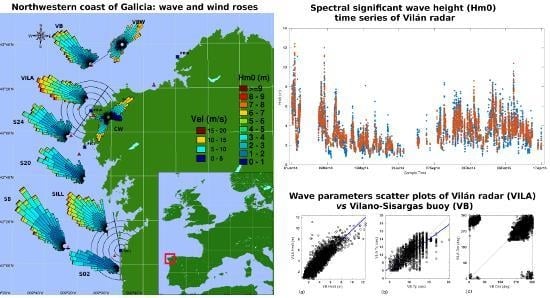
28]. The radars, the objective of this project, are part of the HF radar network deployed on the Galician coast (
Figure 1), consisting of four HF radars working with a frequency of 4.86 MHz, by which the highest saturation limit is 24 m [
29], but for the signal of the second order peaks, rising over the noise floor, the minimum wave height can be larger depending on the situation; hence, these radars work better with high waves than with small ones [
14,
30]. Besides, waves should have at least a period of 5 s, or longer if the noise floor raises, to be interpreted by the radar [
25].
Previous validation of wave data from the Galician radar network concluded that Silleiro radar Hm0 is in good agreement with buoy data, but also reflected some problems estimating Tc when bimodal sea state occurred [
31]. On the other hand, Lorente et al. [
30] showed, for a longer data time series, some differences in wave height estimation between the HF radars from Silleiro and Vilán and the closest buoys, which could be due to the influence of some oceanographic conditions, such as tides, currents and bimodal sea states, and also differences in wave direction probably induced by the depth at areas close to the shoreline. This work also revealed that the deviation of the wave direction was different for each radar.
Considering these factors, the complex weather and the characteristics of the Galician coast, our study aims to elaborate an exhaustive methodology for describing and interpreting the reliability of wave parameters estimated by the Silleiro and Vilán HF radar sites, so their data may be used directly by the end-users.
Thus, all radars’ spectra were re-processed; then, the types of wave regimes not measured by the radars were identified, and the new clean wave data for the ten range cells were validated with nearby buoys. The weaknesses and strengths of the radar estimations for the usual wave regimes of the area were established. In order to support the discussion of the results, the wave regime of the area was described by employing the Hm0 and Dm calculated by in situ wave-gauges and reanalysis modeling data at different locations along the coast.
Additionally, we attempted to update the present methodology for wave data screening defined by the Copernicus Marine In Situ Team [
32] in the framework of the Copernicus Marine Environment Monitoring Service (CMEMS). Such screening does not include a method to deal with wave products from HF radars. Finally, we were able to reduce by one hour, the wave spectrum processing time.
2. Materials and Methods
The radars selected for the analysis were the Vilán radar (VILA), owned by Intecmar-Xunta de Galicia and the Silleiro HF radar (SILL) owned by Puertos del Estado (PdE). Both are long-range CODAR SeaSonde HF radars, composed of 2 antennas deployed only a few meters apart: one is for emitting and other is a composition of 3 crossed antennas that independently receive the backscatter signal, which is used during the wave direction-finding process. The working frequency is 4.86 MHz, and the transmission signal’s sweep width is ≈29.41 KHz. The backscatter signal is spatially solved into concentric rings around the radar location, named range cells (see
Figure 1). These are 5 km thick, which is the spatial resolution defined by the sweep width [
16]. Thirty minutes of the received signal are processed by the proprietary CODAR software into Doppler cross spectra which are saved in files named CSS (CrossSpectra Short time) [
33]. Then, by means of the inversion fitting with the Pierson-Moskowitz model and a cardioid directional factor, a pre-fixed sampling period, defined by a certain number of CSS files, is used to calculate the wave directional spectrum [
22].
For this work, CSS files from January, 2014–April, 2015 were re-processed using an update of the release 7 of the CODAR SeaSonde software, and the following configuration was applied:
Selection of sampling period to be introduced in the model fitting, which will determine the delayed time between the wave detection and the equation of the spectral wave parameters—Tc, Hm0 and Dm. The CSS files of Vilán radar were processed twice, using 180 and 120 min. Silleiro radar CSS files were processed over 180 min.
The periodicity of the resulting wave parameters was fixed to thirty minutes.
Definition of coastline limits (CL) of the coverage area, and the wave bearing limits (WB) according to the shoreline and the open sea surrounding the radar. In this case, due to the coastline facing open sea and the waves from land being considered negligible, CL and WB coincide. Hence, for Vilán radar these were fixed to 221° and 41° (all directions are defined as clockwise from the true north) and for Silleiro radar to 180° and 350°. On the other hand, to define the range, the number of range cells was fixed to ten. Since the first 5 km from the radar’s location are not included in the sampled area, the total radar range is 55 Km.
Minimum and maximum wave period were fixed to 5 and 17 s, following CODAR recommendations [
33].
The resulting wave parameter data sets were screened by a method based on the quality control for waves developed by the Copernicus Marine In Situ Team [
32]. The update consisted of taking into consideration the enormous number of samples flagged as nulls by the radar software to detect stuck values and jumps.
Within the HF radar’s footprint are two permanently deployed SeaWatch buoys (
Figure 1), which were deployed by PdE: Vilano-Sisargas buoy (VB), 40 km to the north of Vilán Cape, and Silleiro buoy (SB), 60 km in front of the Silleiro radar. These buoys take motion measurements for twenty six minutes and generate spectral wave parameters files each hour [
34]. For this work, mean direction (Dm), peak direction (Dp), peak period (Tp) and spectral significant height (Hm0) were used to validate the HF radars’ wave parameters. Besides, the mean wind velocity and direction measured by Vilano-Sisargas buoy were also used (VBW,
Figure 1).
For the wave regime description all through the coverage area of both radars, wave data from three SIMAR points were used: 3002024 (S24); 3004020 (S20) and 3014002 (S02) (
Figure 1). These are part of the subset WANA, based on the reanalysis of the WAM and WaveWatch models run by PdE. The final products are four data sets of hourly basis spectral wave parameters: one extracted from the total wave spectrum, two from the spectra of two possible swells and one from the wind waves spectrum [
35].
Wind data from Camariñas meteorological station (CW,
Figure 1) were obtained from MeteoGalicia weather service [
36].
All data sets were time paired on an hourly basis. The validation of the radar wave parameters was carried out mainly by computing the Pearson correlation index (R); the mean absolute percent error (MAPE); the root mean squared error (RMSE); the bias; and in the case of the wave direction, the circular R and circular mean absolute error (MAE).
The collected data spans from 30 January 2014–30 April 2015. However, the abundance of samples from each device is different due to the deployment schedules or malfunctions during operation. Hence, here are some relevant sampling gaps: 1–19 August 2014; 31 January–2 February 2015; and 31 March–9 April 2015—probably due to a VILA malfunction. 17 January–20 February 2014; and 21 April–22 July 2015—due to a break on VB deployment. Finally, a gap from 21–25 August 2015 in the SILL data set.
3. Results and Discussion
Former validation of VILA range cell at 25 km (RC 25 km) and Vilano-Sisargas buoy Hm0 by Lorente et al. [
30] revealed a consistent correlation. However, radar wave data had a lot of outliers which had a high impact in the statistical results (R ≈ 0.75). Hence, for this work, VILA data were re-processed with a more recent release of the radar’s software which is more accurate, producing fewer outliers. Moreover, the screening applied increased the number of outliers detected; hence, R got a value of ≈0.88 for the same range cell.
Figure 2 shows the good agreement between the VILA Hm0 time series for RC 10 km and the corresponding buoy paired data. However, there are many gaps which extend from some hours to many days that do not correspond to the operation gaps described in the previous section.
Table 1 shows that the highest loss of data corresponds to radar samples flagged as nulls by the software, which in some cases can reach more than 70% of the samples. This flagging occurs when the number of backscatter Doppler points are not enough for accurately calculating the Doppler spectrum, and hence the wave parameters [
33].
3.1. Analysis of HF-Radar Data Loss
Such a percentage of radar samples represents a great loss of the wave information that will be excluded from the statistical analysis. With the aim of finding out whether there is any trend in this loss besides the operational limits of the radars, a correlation between these nulls and the wave regime described by the related samples of the buoys was carried out.
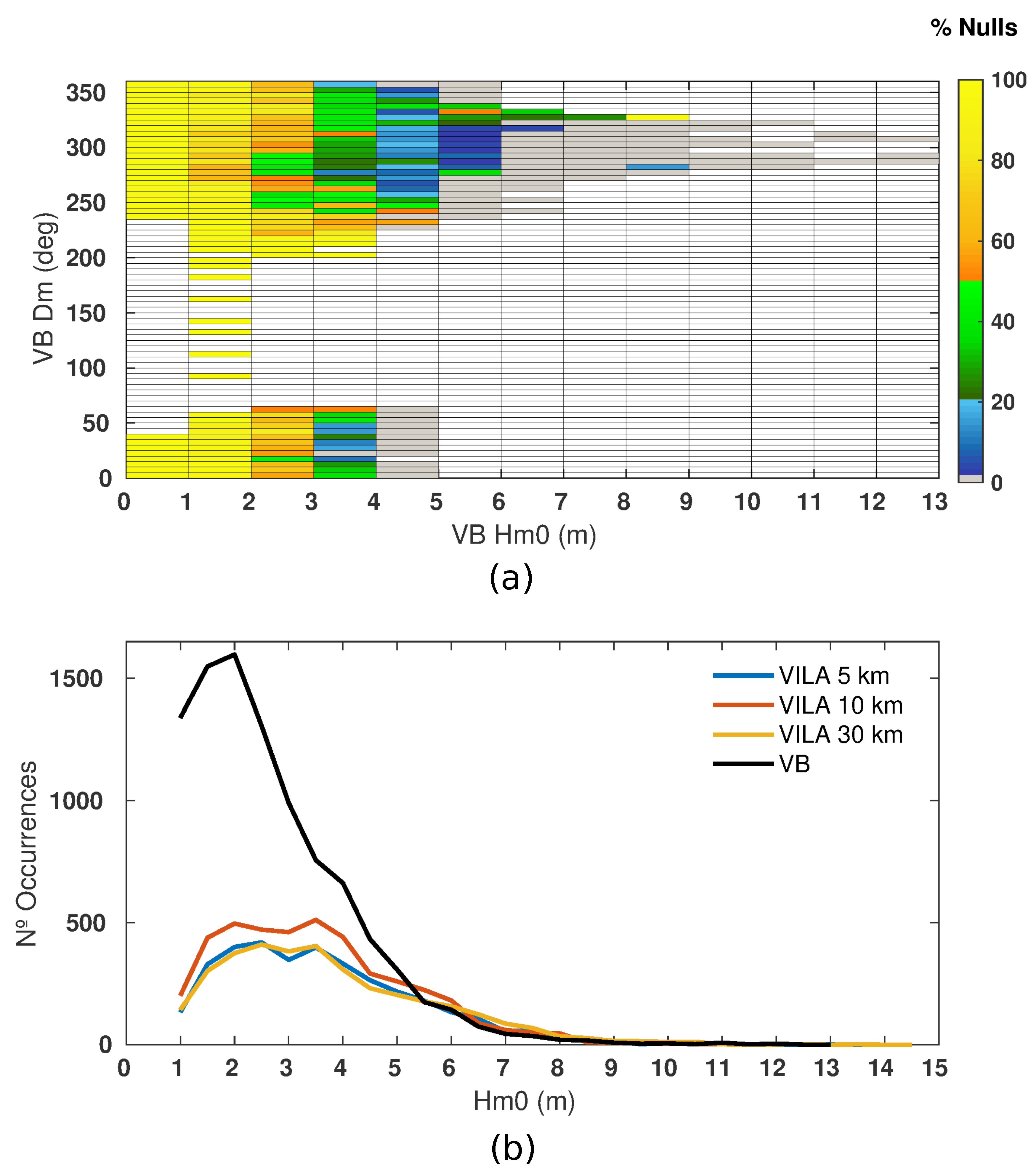
The results of VILA case, represented in
Figure 3a, shows a strong correspondence between the loss of data and the waves between 1–3 m, but also for the higher waves. Since the absence of Doppler points mostly happens when the second-order peaks cannot surpass the noise level, the small waves are more susceptible to not being detected by the radar. Another possibility is that the noise level increases, masking then, the signal, even for waves larger than 2 m [
24]. The histogram (
Figure 3b) shows how relevant this loss is, especially for waves from 2 to 4 m in height, and the displacement between the modes of the VILA and VB Hm0 values. Except for RC 5 km, increasing the distance to the radar increases the data loss (
Table 1). This could be due to a decreasing of the strength of the backscatter signal with the distance. In contrast, the furthest range cells describe slightly more waves higher than 6 m, probably as a result of the sea state heterogeneity around the range cells, or more likely due to the radar’s software trend to produce more Hm0 outliers at the furthest range cells (see screened outliers in
Table 1).
SILL nulls are 20% less than for VILA case, and correspond mostly with waves smaller than 2 m, and in lower percentages to higher waves (
Figure A1).
3.2. Wave Parameters Validation in Terms of Radar Range Cells
Validation of wave parameters was examined between paired samples of VILA and VB excluding the radar nulls and other errors detected during the screening, so more than 50% of the wave information was not included in the statistical analysis.
Figure 4a–f show wave validation for each range cell data set. Note that for the range cells from 10–30 km there is a strong Hm0 correlation, with R ≈ 0.88 (a) and low MAPEs (b). The value of R for the last four range cells falls to 0.78 (a). Albeit the linear correlation between the periods is not so high (≈0.7), the MAPEs remain below 12%(c, d). Regarding Dm, circular R remains below 0.7 for all range cells, but again, mean errors are small, with all MAEs remaining below 26° (e, f).
Although the differences between the values of these statistical parameters are small, in most cases discrepancies between the radar and the buoy increase after RC 30 km, which coincides with the last range cell recommended by CODAR for the long-range radars [
33].
However,
Figure A2 shows that further from the coast, differences between Silleiro radar and Silleiro buoy do not increase. Moreover, the correlation of Dm values improves with distance, probably because the farthest range cells are more exposed to the open sea and have less influence of the coastline, which is less rugged compared to VILA site.
Further validation of wave parameters was focused on VILA RC 10 km, as it is the one with the highest number of samples and highest agreement with the buoy data. This distance from the coast is also the area with more potential for fishing and marine activities (leisure, renewable energy, etc).
Figure 5a–c show the regression lines between VILA and its corresponding VB wave parameters. The regression line for Hm0 has a very small intercept and slope, which reinforces the significance of the value of R ≈ 0.88 (a). However, data dispersion is relevant, and some spurious points can be detected. Besides, after pairing the two data sets, all the buoy values below 1 m have been excluded; therefore, all the radar waves below 1 m are underestimated when compared to buoy data. Moreover, the largest buoy waves are also underestimated by the radar. Linear regression of the wave periods (b) results in a smaller but relevant R ≈ 0.78; however, in this case, the intercept is larger due to the minimum radar operation period of 5 s; the scatter plot describes also a radar underestimation of many buoy periods between 10 and 15 s.
The circular correlation index of Dm only reaches 0.66 (
Figure 5c). The most relevant differences occur when the buoy describes north and northeast wave directions, while the radar shows northwest directions. There is also a significant southwards deviation in the radar estimates which includes an accumulation of points at the south radar coastline limit (221°).
In general, validation of Silleiro radar with Silleiro buoy described a slightly lower correlation than VILA with VB for the three wave parameters (
Figure A3a–f), especially, as Lorente et at. [
30] described, the correlation between periods (c). Here, the southwards trend of the radar Dm values is very noticeable (c). The exclusion of 2014 winter had a relevant influence on these results when compared to those by Lorente et al. [
30].
These Hm0-R values are similar to those described in earlier validation works of SeaSonde HF radars, such as Long [
26] with a 12–13 MHz SeaSonde (R ≈ 0.85–0.91), and Alfonso [
31] who validated winter-period wave data of Silleiro radar (R = 0.89). Another HF radars, with a work frequency of 25 MHz, described a slightly smaller correlation (R ≈ 0.65–0.71 [
25], R ≈ 0.78 [
27]). In general, the agreement between HF radars and buoy periods is difficult since the radar centroid period does not coincide either with buoys Tp or Tm [
4]. Long and Saviano’s works [
26,
37] compared Tc with Tm and Tp, demonstrating that Tc takes values between the two of them. Regarding wave direction, the method used by these radars, the direction-finding, is conditioned by the cardioid model [
14] and by an accurate antenna pattern measurement [
38]. In addition, and as it is explained later, in general, the three parameters are conditioned to an unimodal sea state and an assumed uniformity through all range cells.
3.3. Wave Regime Description
The explanation for most of the observed differences between the radars and the buoys data can be climate-related or related to the different measuring and wave spectra computing methodology of each device. To clarify the incidence of these causes, the wave regime of the area has been analyzed using available wave data sources.
Coastal wave regime, in contrast to the previous validations, is based on the “time paired raw samples” (
Table 1), so all data sets describe the same sampling period and size (9634 samples). Since radars nulls are included, the wave regimes described by them have less information than the other data sets.
In general, the wave roses shown in
Figure 1 describe three main wave regimes: NW regime, which includes all ranges of wave heights, and it is clearly the dominant in this region; the NNE regime, with small and medium-size waves; and the SW regime. Focusing on the specific data sites, NNE waves are only well described by VB, whose location was exposed to be the Cantabrian sea, so any other data source located southern from this position will shade the NE waves’ contribution. Additionally, the NW waves change their approaching angle when getting close to the coast. Hence, other data sources such as S20 and S02 describe these with a more western direction than VB. Therefore, S02 practically does not detect NNE wave systems and estimates most of the NW waves as almost westerly. Regarding the SW wave regime, whilst the buoys only describe small and medium-size waves, the SIMAR points show the occurrence of some high waves. In contrast, VILA clearly underestimates both NNE and SW wave regimes, except for a saturation at its southern CL. On the other hand, SILL does not describe even the northerly waves because its northern CL is limited to 350°, and it underestimates the SW wave regime, except, as well as VILA, for the saturation at its southern CL.
Although VILA shows a considerably higher proportion of extreme waves than the others, especially than the SIMAR points, this is mainly due to most of the small waves not being included in the radar wave roses, so the relative proportion of the higher waves becomes larger. This can be observed in
Figure 6 for the VB wave rose, calculated with samples not paired with radar nulls, which describes a smaller relative abundance of the NNE and SW wave regimes but larger NW regime. Moreover, the NW wave regime becomes more westerly, like the radar one. Besides, when an extreme wave condition occurs, the SIMAR model tends to underestimate the wave height [
35].
The presence of wind waves and swell in the area influences both radar and buoy wave-parameter calculations, due to the existence of a broadband sea state, or even more, a bimodal sea state by which there is more than one wave regime at the same time. These complex sea states are not accurately described by the spectral wave parameters, since these are the result of integrating or averaging the wave spectrum. For the HF radars case, this could induce more inaccuracy because the wave spectrum is fitted to an unimodal wave model [
23,
24]. Moreover, since the radar computes the spectral parameters using the backscatter signal for a whole range cell, if some zones have different exposure to the wave regimes or to a complex sea state, the final wave parameters will be average values [
4]. In other cases due to the radar location and operation, parts of the wave spectrum could be outside its range by their directions, by their frequencies or by their energy, so the radar would not use the whole wave spectrum during the calculations of the wave parameters.
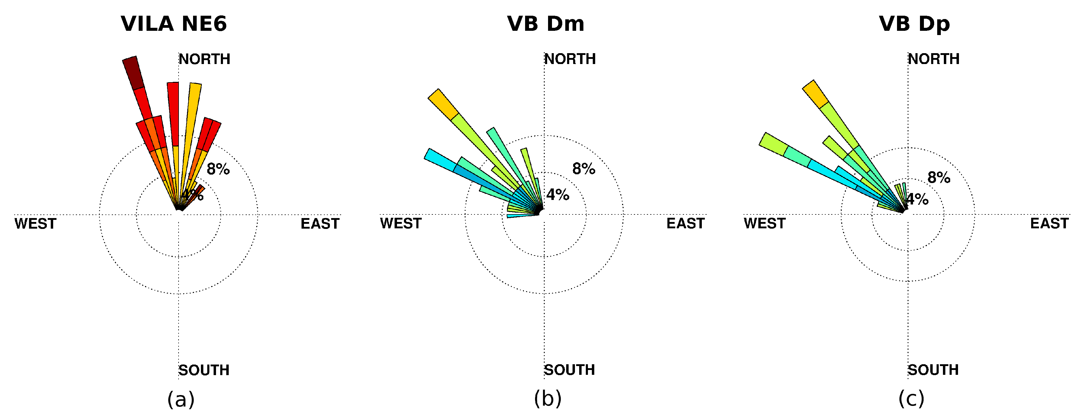
To gain insight into the observed differences between radar and buoy wave-parameter calculations, two examples of typical wave spectra obtained from Vilano-Sisargas buoy are shown in
Figure 7a,b. In the first case (a), two peaks with similar energy and different wave directions are averaged by the buoy to get a Dm of 245°, similar to the value obtained by the radar (269°). For both devices, their wave spectra describe all the wave regimes at that time. However, for the second case (b), the Dm values obtained by the buoy and radar are quite different (2° and 321°, respectively). As the radar does not “see” NE wave contributions, the Dm is closer to the main peak direction. If the same comparison is done with the SIMAR point S24, located at the south of the radar footprint, the Dm of S24 swells (292°, 331°) gets values close to the NW directions of the buoy spectrum; however, the Dm of the S24 wind waves (15°) remains closer to the true north than to the NE peak of the buoy spectrum (≈50°).
3.4. Wave Parameters Validation in Terms of Wave Regimes
For further validation, for each of the three wave regimes described for Vilano-Sisargas buoy, we have selected three wave height intervals: wave heights below 2 m to account for those considered by the radar software as nulls; between 2 and 6 m, which account for the most frequent wave heights; and finally, wave heights larger than 6 m (see
Table 2 for a quick description of the nine wave regimes).
We have validated Vilán HF radar wave data with these nine buoy wave regimes (
Table 3). Additionally, we have re-calculated and validated the nine wave regimes in terms of the radar data (
Table 4), for comparison and for a deeper comprehension of the HF radar operation and the reliability and utility of its estimates.
3.4.1. Buoy Wave Regimes
As shown in
Table 3, many types of wave regimes do not have enough data for validation due to the high number of null radar data. In addition, SW6 and NE6 regimes are practically non-existent for the buoy. Statistical analysis of the remaining regimes reveals a high correlation of Hm0 for waves between 2 and 6 m with NW and SW directions (R ≈ 0.8, MAPE < 20%). However, for the NE waves, the differences between the buoy and the radar are greater, especially for Dm, due to these waves being able to be outside of the radar range (
Figure 7b). For higher waves (NW6), Hm0 shows a low correlation but also a very low average error, and a good agreement with Dm, compared to the other wave regimes. The smallest waves are only represented in the NW2 type that barely retains 20% of the samples, and its concordance with radar estimates is very low for the three wave parameters.
3.4.2. Radar Wave Regimes
Since buoy and radar data sets describe significant differences regarding Dm, the nine wave regimes in terms of the radar data are quite different in size when comparing the buoy ones, but also regarding the result of their validation, which requires an in-depth analysis.
Note in
Table 4 the low correlation and large MAPE and MAE values for NE2, and especially for NE6. For the NE2 case, wave heights are significantly underestimated if compared to buoy data (Bias −0.96 and RMSE 1.12 m) and include north-northwesterly waves, while related buoy waves are mostly northeasterly. In
Figure 8c can be seen that this buoy wave directions is mostly out of reach of the radar range (Dp > 41°). Something similar is observed for NE4 regime (more details in
Figure A4(2) in the
Appendix A, where the rest of the wave roses of the nine wave regimes are also displayed). On the other hand, the large errors obtained for NE6 regime for wave height and direction (
Figure 9) correspond to the spurious values shown in the scatter plot (
Figure 5a). This wave regime seems to aggregate relevant errors in radar estimation, which are shared among many of the buoy wave regimes.
Wave regimes NW4 and NW6 show a good Hm0 correlation with the buoy estimates and low errors for T and Dm. In
Figure A4(5,6), the wave roses are similar for the buoy and the radar, except for the radar tendency to overestimate Dm westwards.
Regarding SW wave regimes, although the Dm errors are high (MAE ≈ 35°), and only SW4 shows a relative strong Hm0 correlation, for the whole SW regime this is very significant (R ≈ 0.89), as it is for the samples responsible for this large disagreement between Dm estimates.
Figure A4(7–9) show differences between buoy and radar Dm which are too high to be explained by the radar tendency to overestimate Dm westwards. Furthermore, the buoy wave rose in
Figure 10c shows that the most energetic waves are mostly from the NW.
Thus, we performed an additional comparison between VILA SW wave regimes and wind data from Camariñas meteorological station (CW), which revels that the Dm differences occur for winds from NW and NE (
Figure 11a), that support the buoy Dm estimates.
However, a further analysis of the saturation of radar samples at 221°, reveals that this mainly occurs during strong southerly winds (velocity>10 m/s, direction ≈ 180°,
Figure 11b), so this seems to follow the wind. The corresponding buoy samples describe W-SW waves, and again the Hm0 correlation between both data sets is high (R ≈ 0.9).
The wave regime validation performed on the Silleiro radar outcomes revealed an aggregation of large Hm0 and Dm errors for a specific wave regime (Hm0 > 4 m and Dm between 180°–235°,
Figure A5) which corresponds to the red points of the scatter plots in
Figure A3a–c.
3.5. Reduction of Data Processing Time
Figure 12 shows the statistical comparison of VILA and VB wave parameters, using 120 or 180 min of CSS files to calculate the wave spectrum during VILA operation. Note that the difference between both data sets validation is less than 3% for all the wave parameters.
Validation of wave parameters for RC 10 km as a function of the nine wave regimes defined in the previous section is shown in
Figure 13. Again, the differences observed for all the statistics are small.
However, processing with a time range of 120 min increases by 3% the number of samples flagged as null by the radar’s software.
4. Conclusions
In this work, the accuracy of the wave data generated by Vilán and Silleiro HF radars (VILA, SILL) have been thoroughly analyzed considering the characteristics of their coverage areas. Radar cross spectra files from Jan 2014–April 2015, were reprocessed using the same last update of the R7 of CODAR SeaSonde software. This software improved the quality of the VILA-derived wave parameters compared with those estimated in situ with previous software versions [
30]. Besides, an updated screening method based on CMEMS recommendations was implemented, which helped to detect outliers among extensive periods of null data.
Data analysis revealed that VILA generated nulls samples for all the waves with spectral significant height (Hm0) ≤1 m; most of the waves <3 m; about half of waves between 3–4 m; and about 10% of those between 4 and 6 m coming from the north-northwest. These percentages of nulls increased with the distance to the radar. SILL produced 20% fewer nulls than VILA, which mainly corresponded to waves below 2 m. This vast number of nulls cannot be completely justified by the HF radar limitations, even less so when SILL has significantly fewer nulls than VILA. Therefore, other factors could be affecting signal reception.
The analysis of the remaining no null HF radars data, revealed that VILA produces reliable wave parameters for the first six range cells—until 35 km—and SILL until 55 km, improving its agreement with Silleiro buoy, especially regarding mean direction (Dm), with the distance to the coast.
Further validation of VILA range cell at 10 km revealed that the best agreement with the buoy occurs for waves between 2 and 6 m coming from the northwest (Hm0-R ≈ 0.8) and that the radar tends to underestimate the biggest and the smallest waves—Hm0>8 m and between 1 and 4 m respectively. Regarding Dm, VILA tends to allot more westward directions than the buoy to the NW wave regimes—more perpendiculars to the shoreline—and the waves that the buoy estimates with NE direction are interpreted as NNW directions by the radar.
The specific analysis of the VILA-derived wave regimes revealed that waves with Hm0 > 6 m and Dm between 330° and 45°—clockwise—correspond to spurious data. Additionally, VILA southwesterly waves have a strong agreement with buoy estimates regarding Hm0, but in many cases, the buoy estimates NW wave directions. The analysis of the SILL-derived wave regimes revealed that waves >4 m and Dm between 180° and 235° correspond to spurious values; however, ongoing study has revealed that these are less at the furthest range cells. Regarding wave period, both radars underestimated the buoys peak periods between 10 and 13 s, and SILL also overestimated the peak periods between 5 and 8 s.
The most relevant differences between the estimates of VILA and Vilano-Sisargas buoy (VB) have been explained by the characteristics of the wave regime at the western coast of Galicia. This has been described using the wave data of both HF radars, the two buoys and three SIMAR points located in the area. The wave regime is composed of waves from NNE, NW and SW, with different ranges of Hm0 and with a significant variability along the coast, according to their approaching angle and distance to this. For instance, VILA’s coverage area is only partially open to the NE waves—until 41°—and its proximity to the coast induces the perpendicularity—more westwards—of the NW waves. Moreover, as the SIMAR wave parameters and VB wave spectra revealed, in many occasions, these wave systems can be simultaneous, leading to broadband and bimodal sea states which are not accurately represented by the spectral wave parameters estimated either by the buoys or the radars. In addition, the results of the HF radars wave data validation can be affected when part of the buoy’s wave spectrum is out of their range—either very small wave height or period—but also, because the HF radar-derived wave parameters are the average of the sea conditions along each range cell, while the buoys’ estimates are the result of measuring a single point. All these factors also explain some differences between VILA and SILL validation results: SILL’s coast is more straight than VILA’s and is in the shade of NE waves, so the variability along its range cells is lesser than in VILA’s ones. Hence, the proximity of the farthest range cells to the buoy induces more similitude instead of more disagreement, as happens in the VILA area.
This paper has established that VILA and SILL can reduce by one hour, the calculation of the wave parameters, by mean of using fewer samples during the model fitting, assuming an increment of 3% in the null percentage and a slight decrease in the correlation with the buoy estimates.
The method described here is a useful tool for analyzing and classifying the HF radars’ wave outcomes, in order to be interpreted and employed by final users. Additionally, it is useful for detecting whether any adjustment should be done to the radar; for example, to reduce the high percentage of nulls [
39], to avoid the shade to relevant wave regimes or to avoid the heterogeneity of the sea state conditions throughout the range cell. Regarding the last issue, the solution goes through developing new software able to establish different coastline limits for each range cell and solving the wave parameters in shallow waters. Additionally, the development of multi-frequency radars for detecting accurately either small or high waves is necessary [
14,
39]. Finally, new software updates, as described in Lipa [
24], could find the solution for solving complex sea states as bimodals. Additionally, the accuracy of retrieving directional wave spectra could be improved with many published, innovate methods for other HF radar models [
5,
40,
41].

 ,
, 


