Remotely Sensed Land Surface Temperature-Based Water Stress Index for Wetland Habitats

 , , , ,
Abstract
:
1. Introduction
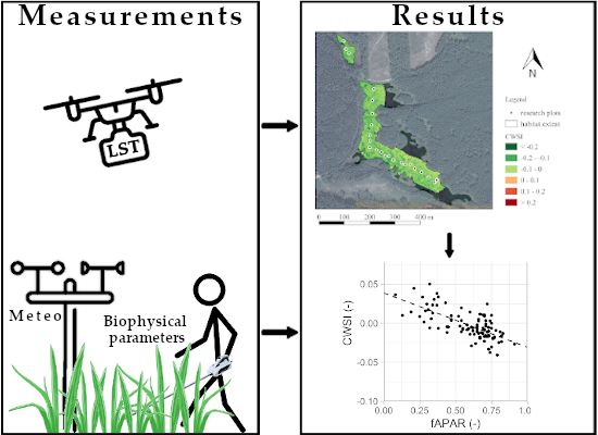
2. Materials and Methods
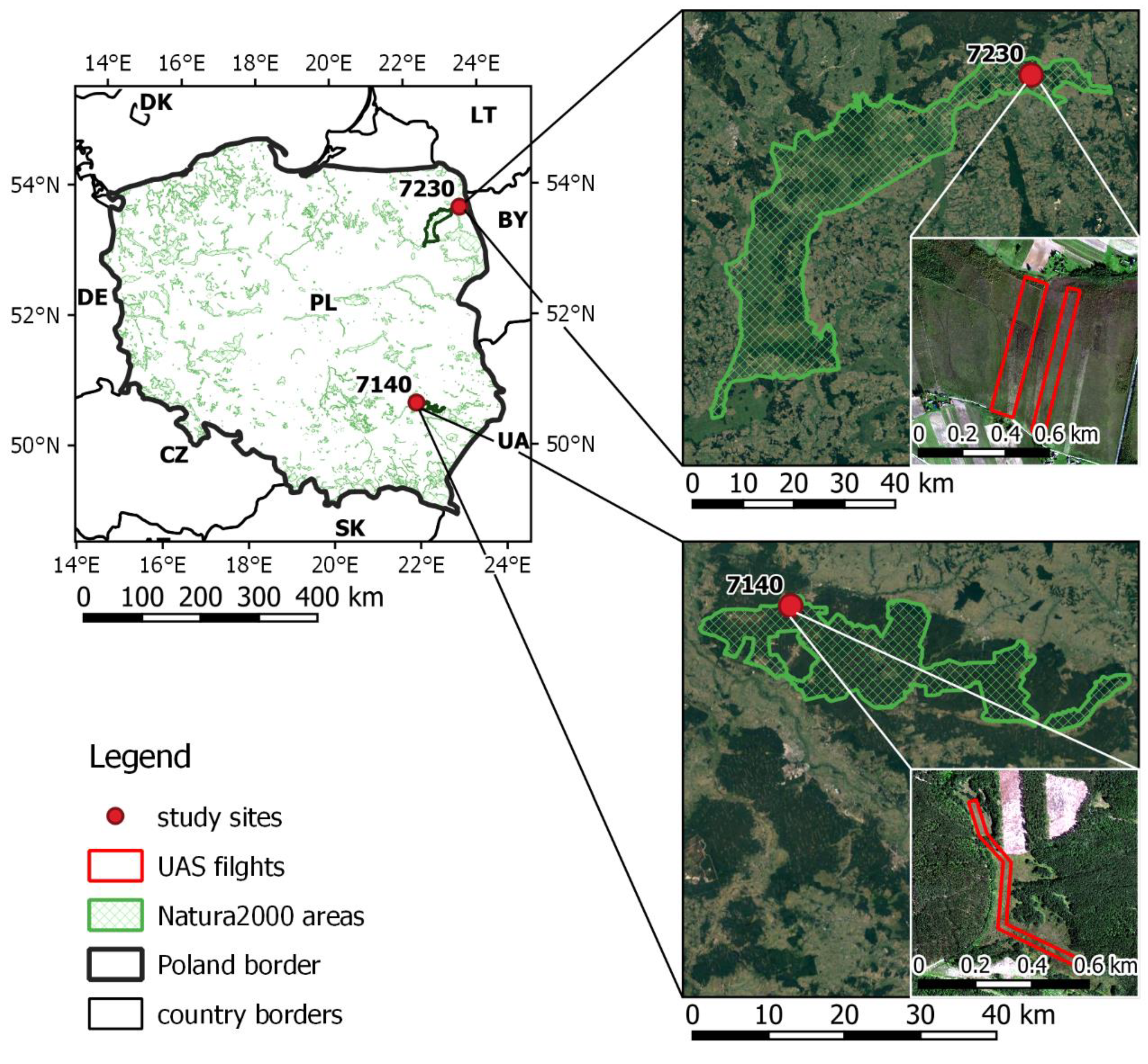
2.1. Study Sites
2.1.1. The Biebrza National Park
2.1.2. The Janów Forest Landscape Park
2.2. CWSI
2.2.1. Formulation
2.2.2. The NWSB derivation
2.3. UAS Data Capture and Thermal Orthophotomosaic Preparation
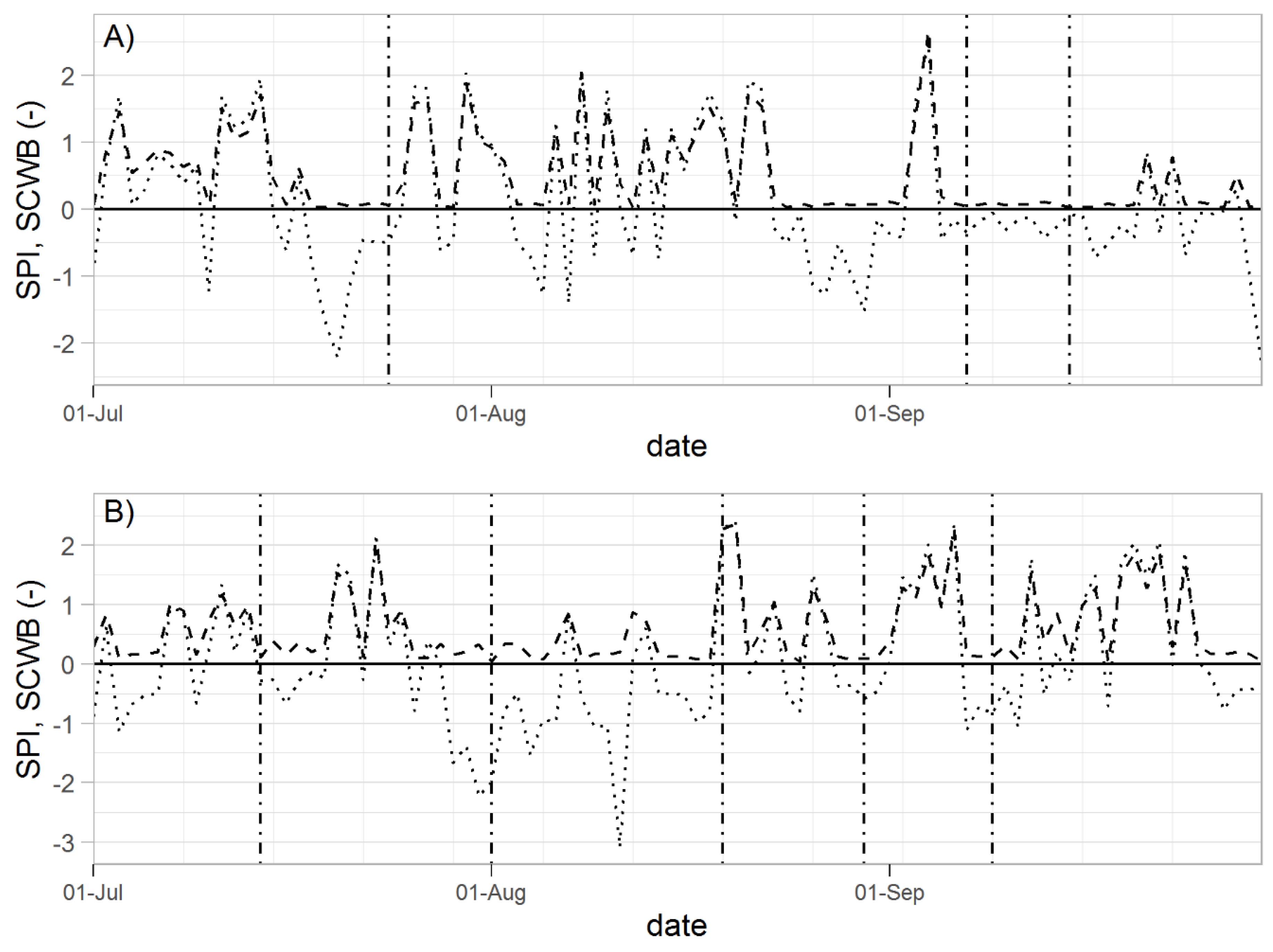
2.4. Meteorological Drought Indices
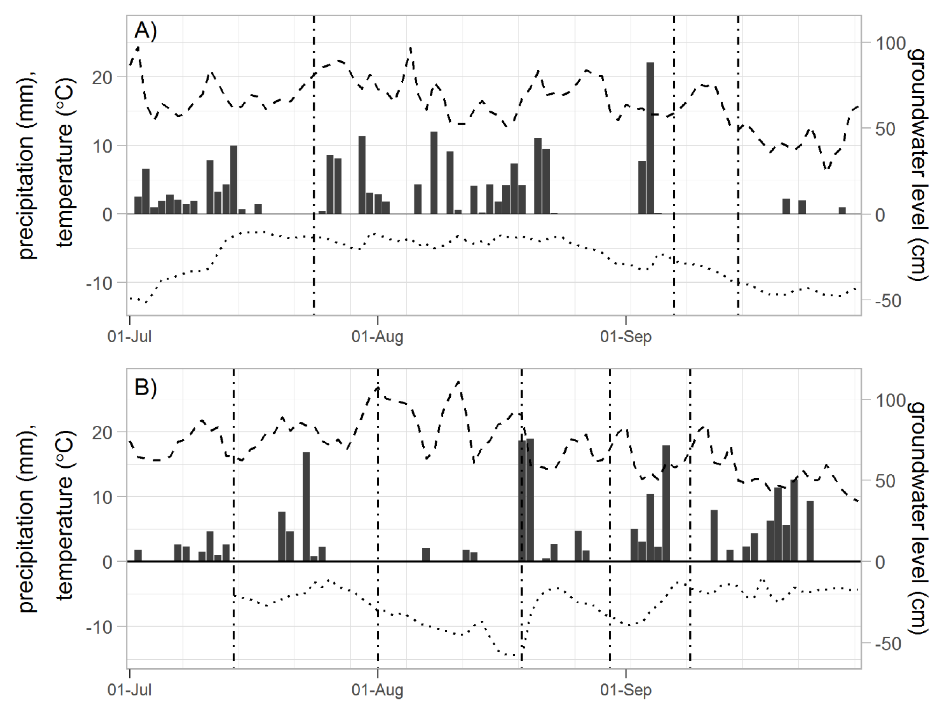
2.5. Biophysical Parameters, Soil Moisture, and Groundwater Level
2.6. Data Analysis
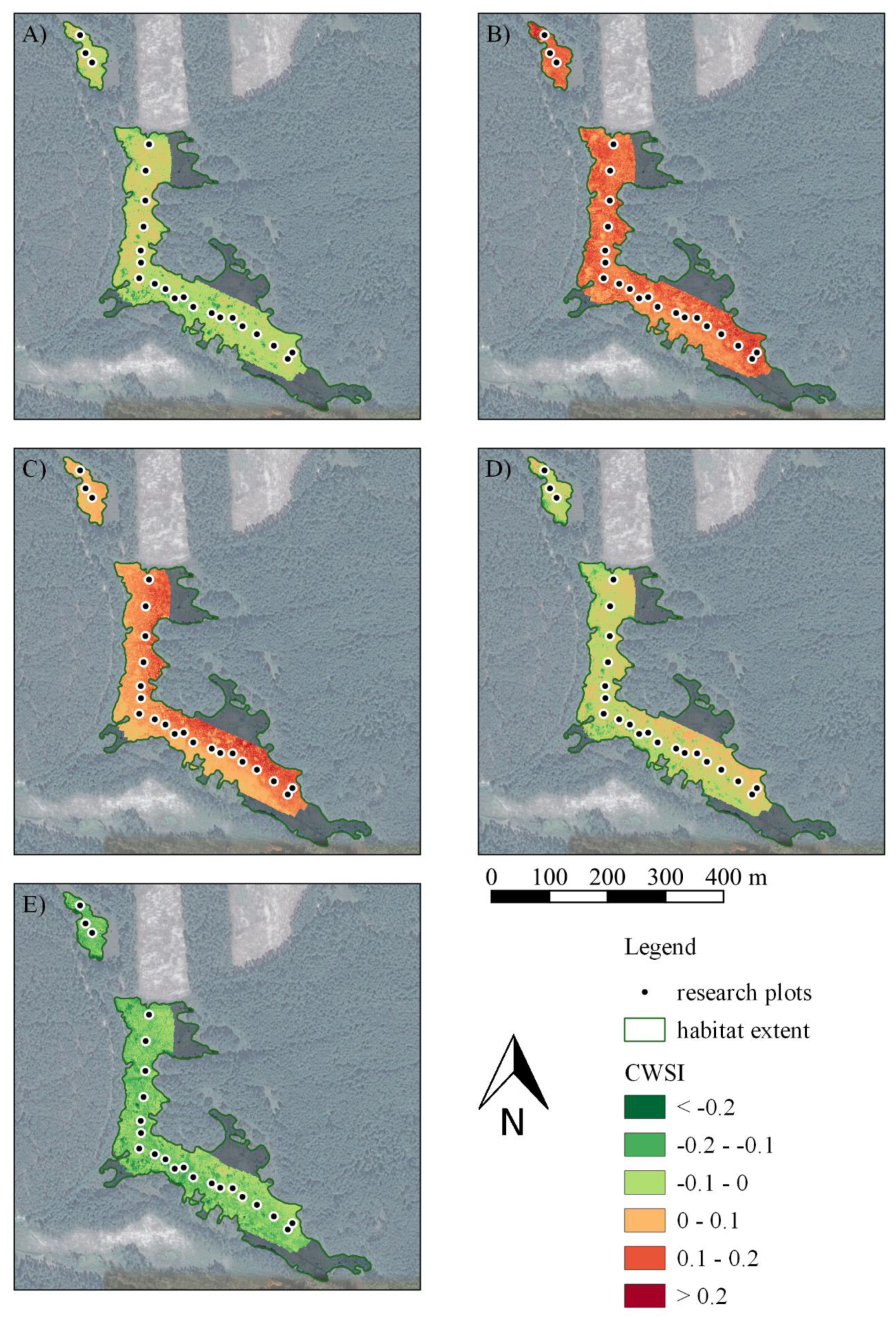
3. Results
3.1. NWSB
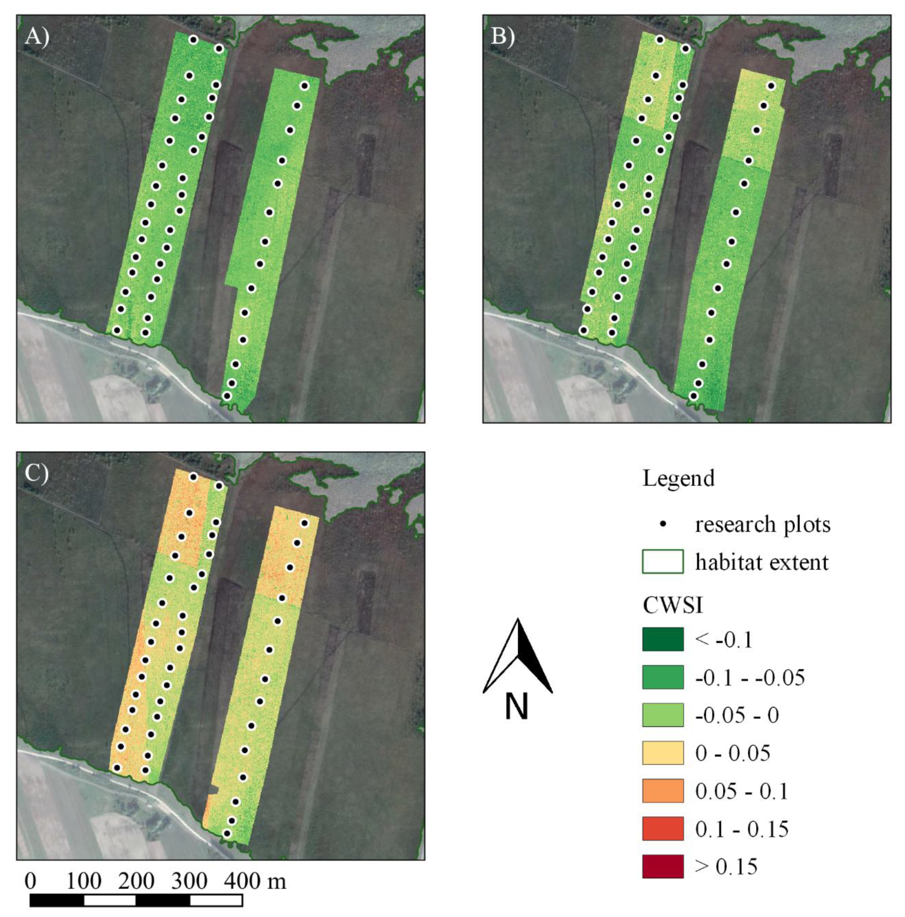
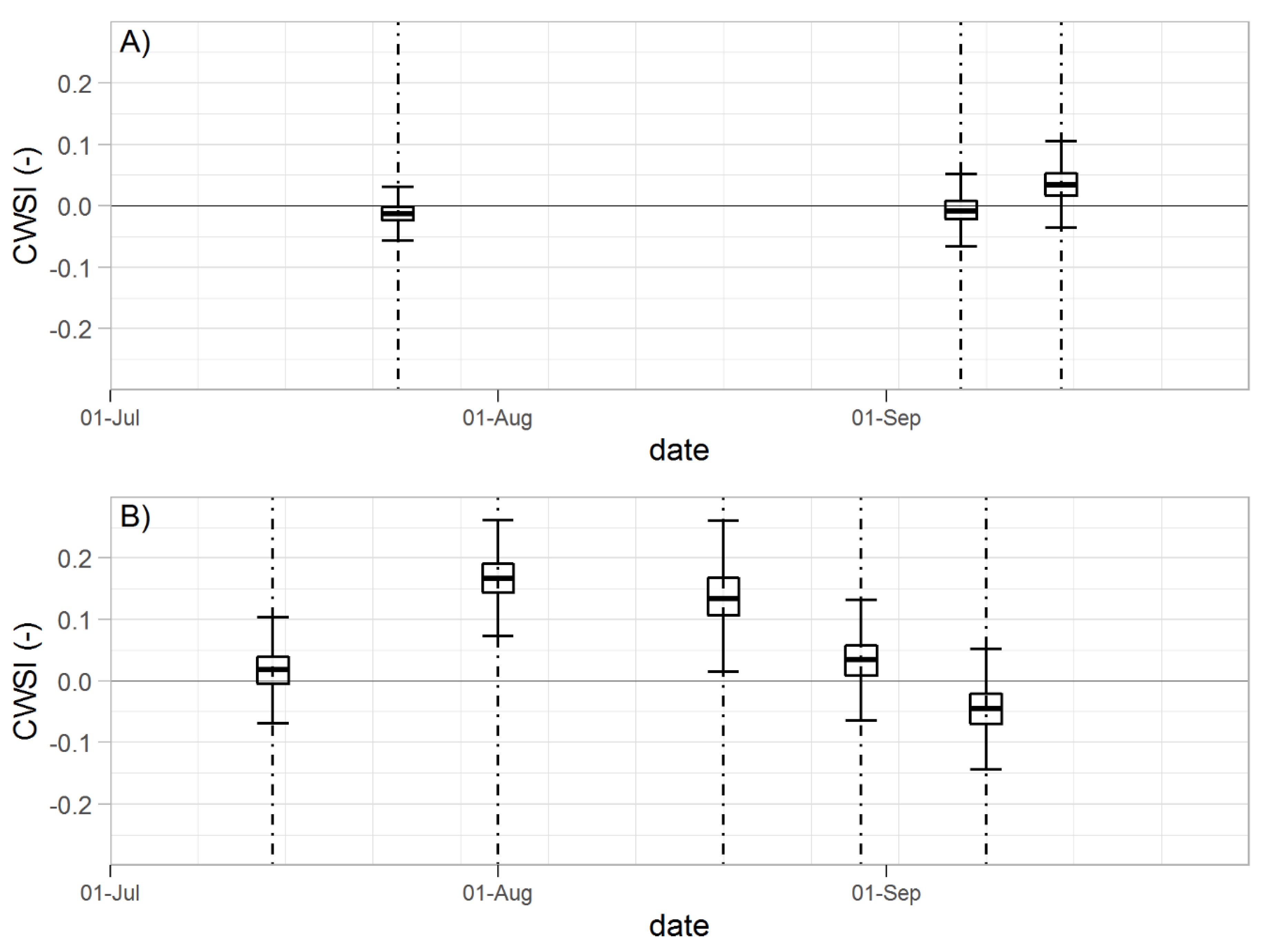
3.2. CWSI
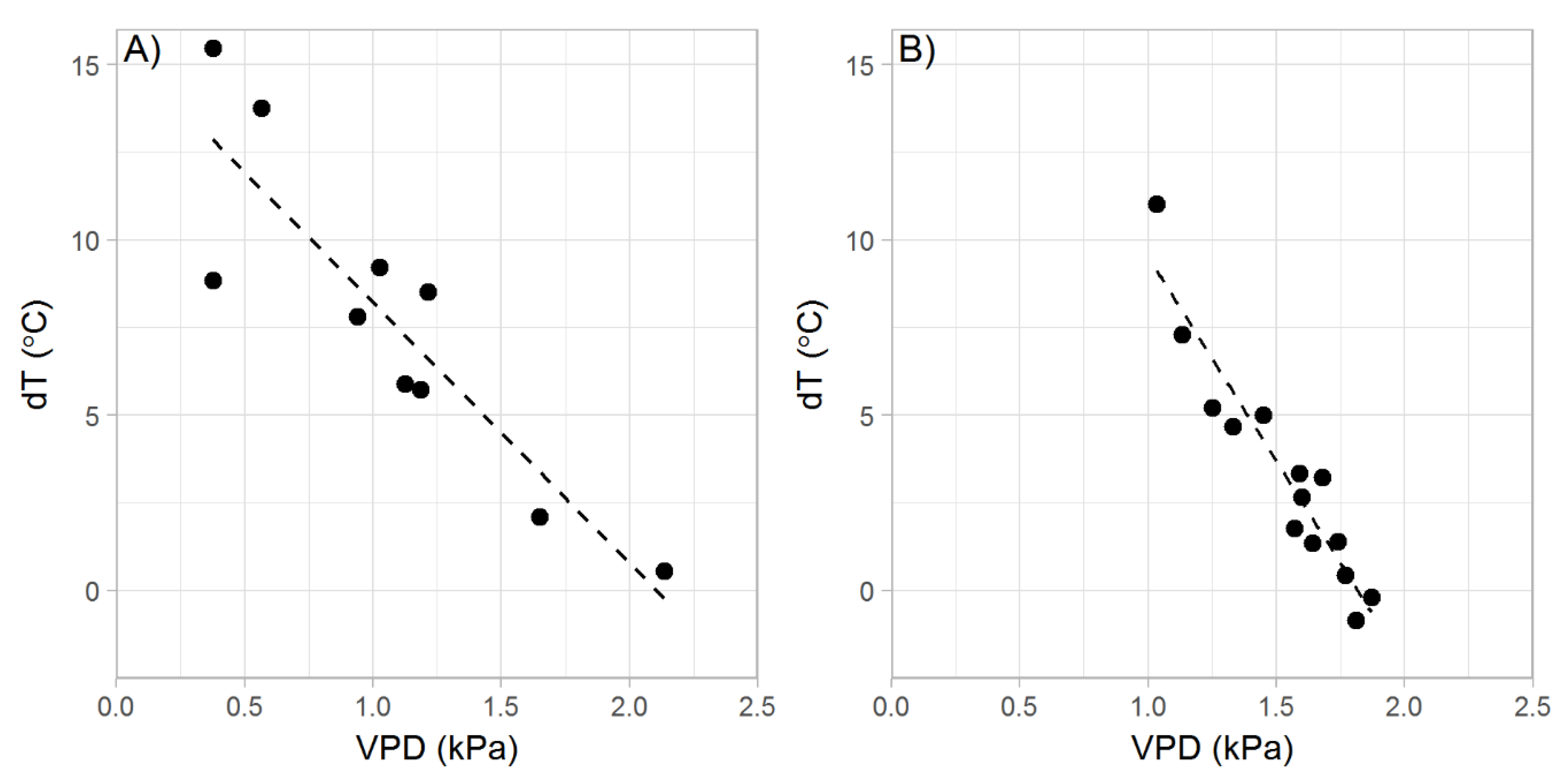
3.3. Meteorological Parameters and Drought Indices
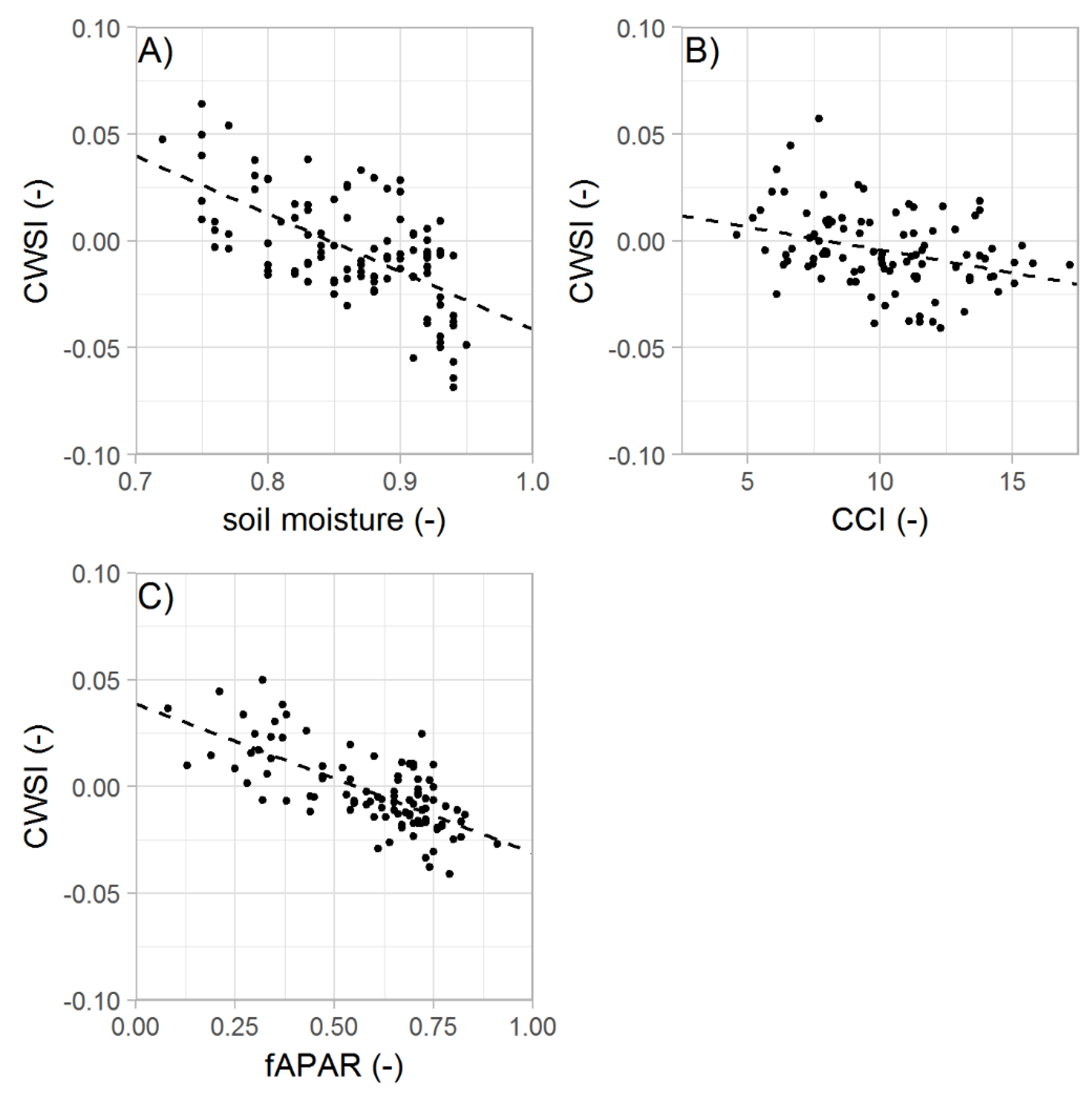
3.4. Correlation of CWSI and Field Measurements
4. Discussion
4.1. The NWSB for Wetland Habitats
4.2. CWSI as Drought Indicator in Wetland Habitats
4.3. CWSI as Water Stress Indicator in Wetland Habitats
5. Conclusions
Author Contributions
Funding
Acknowledgments
Conflicts of Interest
References
- Buringh, P. Organic carbon in soils of the world. In The Role of Terrestrial Vegetation in the Global Carbon Cycle: Measurements by Remote Sensing; Woodwell, G.M., Ed.; John Wiley & Sons: Chichester, UK, 1984; pp. 91–109. [Google Scholar]
- Aselmann, I.; Crutzen, P.J. Global distribution of natural freshwater wetlands and rice paddies, their net primary productivity, seasonality and possible methane emissions. J. Atmos. Chem. 1989, 8, 307–358. [Google Scholar] [CrossRef]
- Barrow, C.J. Wetlands (2nd edn.), W.J. Mitsch and J. G. Gosselink. Van Nostrand Reinhold. Land Degrad. Dev. 1994, 5, 57. [Google Scholar] [CrossRef]
- Gorham, E. Northern peatlands—Role in the carbon-cycle and probable responses to climatic warming. Ecol. Appl. 1991, 1, 182–195. [Google Scholar] [CrossRef] [PubMed]
- Frolking, S.; Roulet, N.T. Holocene radiative forcing impact of northern peatland carbon accumulation and methane emissions. Glob. Chang. Biol. 2007, 13, 1079–1088. [Google Scholar] [CrossRef]
- Yu, Z.C. Northern peatland carbon stocks and dynamics: A review. Biogeosciences 2012, 9, 4071–4085. [Google Scholar] [CrossRef] [Green Version]
- Marshall, C.H.; Pielke, R.A.; Steyaert, L.T. Has the Conversion of Natural Wetlands to Agricultural Land Increased the Incidence and Severity of Damaging Freezes in South Florida? Mon. Weather Rev. 2004, 132, 2243–2258. [Google Scholar] [CrossRef] [Green Version]
- Berezowski, T.; Nossent, J.; Chormański, J.; Batelaan, O. Spatial sensitivity analysis of snow cover data in a distributed rainfall-runoff model. Hydrol. Earth Syst. Sci. 2015, 19, 1887–1904. [Google Scholar] [CrossRef] [Green Version]
- Keizer, F.M.; Schot, P.P.; Okruszko, T.; Chormański, J.; Kardel, I.; Wassen, M.J. A new look at the flood pulse concept: The (ir) relevance of the moving littoral in temperate zone rivers. Ecol. Eng. 2014, 64, 85–99. [Google Scholar] [CrossRef]
- Mirosław-Świątek, D.; Szporak-Wasilewska, S.; Grygoruk, M. Assessing floodplain porosity for accurate quantification of water retention capacity of near-natural riparian ecosystems—A case study of the Lower Biebrza Basin, Poland. Ecol. Eng. 2016, 92, 181–189. [Google Scholar] [CrossRef]
- Berezowski, T.; Partington, D.; Chormański, J.; Batelaan, O. Spatiotemporal Dynamics of the Active Perirheic Zone in a Natural Wetland Floodplain. Water Resour. Res. 2019, 55, 9544–9562. [Google Scholar] [CrossRef]
- Kleniewska, M.; Gołaszewski, D.; Majewski, G.; Szporak-Wasilewska, S.; Rozbicka, K.; Rozbicki, T. Diurnal Course of the Main Heat Balance Components of a Marshy Meadow in the Lower Biebrza River Valley. Polish J. Environ. Stud. 2015, 24, 945–950. [Google Scholar] [CrossRef]
- Ciężkowski, W.; Berezowski, T.; Kleniewska, M.; Szporak-Wasilewska, S.; Chormański, J. Modelling Wetland Growing Season Rainfall Interception Losses Based on Maximum Canopy Storage Measurements. Water 2018, 10, 41. [Google Scholar] [CrossRef] [Green Version]
- Berezowski, T.; Chormański, J.; Kleniewska, M.; Szporak-Wasilewska, S. Towards rainfall interception capacity estimation using ALS LiDAR data. In Proceedings of the 2015 IEEE International Geoscience and Remote Sensing Symposium (IGARSS), Milan, Italy, 26–31 July 2015; pp. 735–738. [Google Scholar]
- Finlayson, M.; Cruz, R.; Davidson, N.; Alder, J.; Cork, S. Millennium Ecosystem Assessment: Ecosystems and Human Well-Being: Wetlands and Water Synthesis; Island Press: Washington, DC, USA, 2005; pp. 30–39. [Google Scholar]
- Fraser, L.H.; Keddy, P.A. The future of large wetlands: A global perspective. In The world Largest Wetlands: Ecology and Conservation; Fraser, L.H., Keddy, P.A., Eds.; Cambridge University Press: Cambridge, UK, 2005; pp. 446–468. [Google Scholar]
- Barros, V.R.; Field, C.B.; Dokke, D.J.; Mastrandrea, M.D.; Mach, K.J.; Bilir, T.E.; Chatterjee, M.; Ebi, K.L.; Estrada, Y.O.; Genova, R.C. Climate Change 2014: Impacts, Adaptation, and Vulnerability-Part B: Regional Aspects-Contribution of Working Group II to the Fifth Assessment Report of the Intergovernmental Panel on Climate Change; Cambridge University Press: Cambridge, UK, 2014; pp. 271–360. [Google Scholar]
- Trenberth, K.E.; Dai, A.; Van Der Schrier, G.; Jones, P.D.; Barichivich, J.; Briffa, K.R.; Sheffield, J. Global warming and changes in drought. Nat. Clim. Chang. 2014, 4, 17. [Google Scholar] [CrossRef]
- Spinoni, J.; Vogt, J.V.; Naumann, G.; Barbosa, P.; Dosio, A. Will drought events become more frequent and severe in Europe? Int. J. Climatol. 2018, 38, 1718–1736. [Google Scholar] [CrossRef] [Green Version]
- Wilhite, D.A.; Glantz, M.H. Understanding: The Drought Phenomenon: The Role of Definitions. Water Int. 1985, 10, 111–120. [Google Scholar] [CrossRef] [Green Version]
- Deverel, S.J.; Ingrum, T.; Leighton, D. Present-day oxidative subsidence of organic soils and mitigation in the Sacramento-San Joaquin Delta, California, USA. Hydrogeol. J. 2016, 24, 569–586. [Google Scholar] [CrossRef] [Green Version]
- Könönen, M.; Jauhiainen, J.; Laiho, R.; Kusin, K.; Vasander, H. Physical and chemical properties of tropical peat under stabilised land uses. Mires peat 2015, 16, 1–13. [Google Scholar]
- Hewelke, E.; Szatyłowicz, J.; Gnatowski, T.; Oleszczuk, R. Effects of soil water repellency on moisture patterns in a degraded sapric histosol. Land Degrad. Dev. 2016, 27, 955–964. [Google Scholar] [CrossRef]
- Wołejko, L.; Pawlaczyk, P.; Stańko, R.; Przyrodników, K. Torfowiska Alkaliczne w Polsce–Zróżnicowanie, Zasoby, Ochrona; Klub Przyrodników: Świebodzin, Poland, 2019; pp. 49–59. (In Polish) [Google Scholar]
- Kluge, B.; Wessolek, G.; Facklam, M.; Lorenz, M.; Schwärzel, K. Long-term carbon loss and CO2-C release of drained peatland soils in northeast Germany. Eur. J. Soil Sci. 2008, 59, 1076–1086. [Google Scholar] [CrossRef]
- Mäkiranta, P.; Laiho, R.; Fritze, H.; Hytönen, J.; Laine, J.; Minkkinen, K. Indirect regulation of heterotrophic peat soil respiration by water level via microbial community structure and temperature sensitivity. Soil Biol. Biochem. 2009, 41, 695–703. [Google Scholar] [CrossRef]
- Khanal, S.; Fulton, J.; Shearer, S. An overview of current and potential applications of thermal remote sensing in precision agriculture. Comput. Electron. Agric. 2017, 139, 22–32. [Google Scholar] [CrossRef]
- Heim, R.R., Jr. A review of twentieth-century drought indices used in the United States. Bull. Am. Meteorol. Soc. 2002, 83, 1149–1165. [Google Scholar] [CrossRef] [Green Version]
- Vogt, J.V.; Somma, F. Drought and Drought Mitigation in Europe. Advances in Natural and Technological Hazards Research; Springer: Dordrecht, The Netherlands, 2000; pp. 167–183. [Google Scholar]
- Gallant, A. The challenges of remote monitoring of wetlands. Remote Sens. 2015, 7, 10938–10950. [Google Scholar] [CrossRef] [Green Version]
- Petrasovits, I. General review on drought strategies. In Proceedings of the 14th International Congress on Irrigation and Drainage, Rio de Janeiro, Brazil, 30 April–4 May 1990; pp. 1–11. [Google Scholar]
- Baier, W. Concepts of soil moisture availability and their effect on soil moisture estimates from a meteorological budget. Agric. Meteorol. 1969, 6, 165–178. [Google Scholar] [CrossRef]
- Gardner, B.R.; Nielsen, D.C.; Shock, C.C. Infrared thermometry and the crop water stress index. I. History, theory, and baselines. J. Prod. Agric. 1992, 5, 462–466. [Google Scholar] [CrossRef]
- Maes, W.H.; Steppe, K. Estimating evapotranspiration and drought stress with ground-based thermal remote sensing in agriculture: A review. J. Exp. Bot. 2012, 63, 4671–4712. [Google Scholar] [CrossRef] [Green Version]
- Irmak, S.; Haman, D.Z.; Bastug, R. Determination of crop water stress index for irrigation timing and yield estimation of corn. Agron. J. 2000, 92, 1221–1227. [Google Scholar] [CrossRef]
- Erdem, Y.; Erdem, T.; ORTA, A.H.; Okursoy, H. Irrigation scheduling for watermelon with crop water stress index (CWSI). J. Cent. Eur. Agric. 2006, 6, 449–460. [Google Scholar]
- Andrews, P.K.; Chalmers, D.J.; Moremong, M. Canopy-air temperature differences and soil water as predictors of water stress of apple trees grown in a humid, temperate climate. J. Am. Soc. Hortic. Sci. 1992, 117, 453–458. [Google Scholar] [CrossRef] [Green Version]
- Wang, D.; Gartung, J. Infrared canopy temperature of early-ripening peach trees under postharvest deficit irrigation. Agric. Water Manag. 2010, 97, 1787–1794. [Google Scholar] [CrossRef]
- Berni, J.A.J.; Zarco-Tejada, P.J.; Sepulcre-Cantó, G.; Fereres, E.; Villalobos, F. Mapping canopy conductance and CWSI in olive orchards using high resolution thermal remote sensing imagery. Remote Sens. Environ. 2009, 113, 2380–2388. [Google Scholar] [CrossRef]
- García-Tejero, I.F.; Rubio, A.E.; Viñuela, I.; Hernández, A.; Gutiérrez-Gordillo, S.; Rodríguez-Pleguezuelo, C.R.; Durán-Zuazo, V.H. Thermal imaging at plant level to assess the crop-water status in almond trees (cv. Guara) under deficit irrigation strategies. Agric. Water Manag. 2018, 208, 176–186. [Google Scholar] [CrossRef]
- Idso, S.B.; Jackson, R.D.; Pinter, P.J., Jr.; Reginato, R.J.; Hatfield, J.L. Normalizing the stress-degree-day parameter for environmental variability. Agric. Meteorol. 1981, 24, 45–55. [Google Scholar] [CrossRef]
- Jackson, R.D.; Idso, S.B.; Reginato, R.J.; Pinter, P.J., Jr. Canopy temperature as a crop water stress indicator. Water Resour. Res. 1981, 17, 1133–1138. [Google Scholar] [CrossRef]
- Pogodynka. Available online: http://klimat.pogodynka.pl/pl/climate-maps/#Mean_Temperature/Monthly/2010/1/Winter (accessed on 30 January 2020).
- Kopeć, D.; Michalska-Hejduk, D.; Berezowski, T.; Borowski, M.; Rosadziński, S.; Chormański, J. Application of multisensoral remote sensing data in the mapping of alkaline fens Natura 2000 habitat. Ecol. Indic. 2016, 70, 196–208. [Google Scholar] [CrossRef]
- Kondracki, J. Geografia Regionalna Polski; Wydawn. Naukowe PWN: Warsaw, Poland, 2000. (In Polish) [Google Scholar]
- Kondracki, J. Geografia Fizyczna Polski; Wydawn. Naukowe PWN: Warsaw, Poland, 1978. (In Polish) [Google Scholar]
- Taghvaeian, S.; Chávez, J.L.; Hansen, N.C. Infrared thermometry to estimate crop water stress index and water use of irrigated maize in Northeastern Colorado. Remote Sens. 2012, 4, 3619–3637. [Google Scholar] [CrossRef] [Green Version]
- Allen, R.G.; Pereira, L.S.; Raes, D.; Smith, M. Crop evapotranspiration-Guidelines for computing crop water requirements-FAO Irrigation and drainage paper 56. FAO Rome 1998, 300, D05109. [Google Scholar]
- TPI. Available online: http://www.tpinet.pl (accessed on 30 January 2020).
- IMGW. Available online: https://danepubliczne.imgw.pl/ (accessed on 30 January 2020).
- McKee, T.B.; Doesken, N.J.; Kleist, J. The relationship of drought frequency and duration to time scales. In Proceedings of the 8th Conference on Applied Climatology, Anaheim, CA, USA, 17–22 January 1993; American Meteorological Society: Boston, MA, USA, 1993; Volume 17, pp. 179–183. [Google Scholar]
- Łabędzki, L.; Bąk, B. Meteorological and agricultural drought indices used in drought monitoring in Poland: A review. Meteorol. Hydrol. Water Manag. Res. Oper. Appl. 2014, 2, 1–12. [Google Scholar] [CrossRef] [Green Version]
- Beguería, S.; Vicente-Serrano, S.M. SPEI: Calculation of the Standardised Precipitation-Evapotranspiration Index R Core Team. 2017. Available online: https://cran.r-project.org/web/packages/SPEI/index.html (accessed on 12 February 2020).
- Jamieson, P.D.; Martin, R.J.; Francis, G.S.; Wilson, D.R. Drought effects on biomass production and radiation-use efficiency in barley. Field Crops Res. 1995, 43, 77–86. [Google Scholar] [CrossRef]
- Gobron, N.; Pinty, B.; Mélin, F.; Taberner, M.; Verstraete, M.M.; Belward, A.; Lavergne, T.; Widlowski, J.L. The state of vegetation in Europe following the 2003 drought. Int. J. Remote Sens. 2005, 26, 2013–2020. [Google Scholar] [CrossRef]
- Jagtap, V.; Bhargava, S.; Streb, P.; Feierabend, J. Comparative effect of water, heat and light stresses on photosynthetic reactions in Sorghum bicolor (L.) Moench. J. Exp. Bot. 1998, 49, 1715–1721. [Google Scholar]
- Nageswara Rao, R.C.; Talwar, H.S.; Wright, G.C. Rapid Assessment of Specific Leaf Area and Leaf Nitrogen in Peanut (Arachis hypogaea L.) using a Chlorophyll Meter. J. Agron. Crop Sci. 2001, 186, 175–182. [Google Scholar] [CrossRef] [Green Version]
- Wright, G.C.; Rao, R.C.N.; Farquhar, G.D. Water-use efficiency and carbon isotope discrimination in peanut under water deficit conditions. Crop Sci. 1994, 34, 92–97. [Google Scholar] [CrossRef]
- Fotovat, R.; Valizadeh, M.; Toorchi, M. Association between water-use-efficiency components and total chlorophyll content (SPAD)in wheat (Triticum aestivum L.) under well- watered and drought stress conditions. J. Food Agric. Environ. 2007, 5, 225–227. [Google Scholar]
- Skierucha, W.; Wilczek, A.; Szypłowska, A.; Sławiński, C.; Lamorski, K. A TDR-based soil moisture monitoring system with simultaneous measurement of soil temperature and electrical conductivity. Sensors 2012, 12, 13545–13566. [Google Scholar] [CrossRef]
- Oleszczuk, R.; Brandyk, T.; Gnatowski, T.; Szatylowicz, J. Calibration of TDR for moisture determination in peat deposits. Int. Agrophys. 2004, 18, 145–152. [Google Scholar]
- Oleszczuk, R.; Gnatowski, T.; Brandyk, T.; Szatylowicz, J. Calibration of TDR for moisture content monitoring in moorsh layers. In Wetlands Monitoring, Modelling and Management; Okruszko, T., Maltby, E., Szatylowicz, J., Swiatek, D., Kotowski, W., Eds.; Taylor & Francis Group: London, UK, 2007; pp. 121–124. [Google Scholar]
- R Core Team. R: A Language and Environment for Statistical Computing. 2019. [Google Scholar]
- DeJonge, K.C.; Taghvaeian, S.; Trout, T.J.; Comas, L.H. Comparison of canopy temperature-based water stress indices for maize. Agric. Water Manag. 2015, 156, 51–62. [Google Scholar] [CrossRef]
- Bellvert, J.; Marsal, J.; Girona, J.; Zarco-Tejada, P.J. Seasonal evolution of crop water stress index in grapevine varieties determined with high-resolution remote sensing thermal imagery. Irrig. Sci. 2015, 33, 81–93. [Google Scholar] [CrossRef]
- Yordanov, I.; Velikova, V.; Photosynthetica, T.T. Plant responses to drought, acclimation, and stress tolerance. Photosynthetica 2000, 38, 171–186. [Google Scholar] [CrossRef]
- Chernetskiy, M.; Gómez-Dans, J.; Gobron, N.; Morgan, O.; Lewis, P.; Truckenbrodt, S.; Schmullius, C. Estimation of FAPAR over Croplands Using MISR Data and the Earth Observation Land Data Assimilation System (EO-LDAS). Remote Sens. 2017, 9, 656. [Google Scholar] [CrossRef] [Green Version]


| Area | Date | Number of Transects | Flights per Transect | Time of Flights | Minimum VPD (kPa) | Maximum VPD (kPa) |
|---|---|---|---|---|---|---|
| Biebrza National Park (7230). | 24.07.2016 | 2 | 3 | 11:00–3:30 | 1.22 | 1.41 |
| 07.09.2016 | 2 | 12:00–2:00 | 1.05 | 1.13 | ||
| 18.09.2016 | 2 | 11:00–2:00 | 1.21 | 1.43 | ||
| Janów Forest Landscape Park (7140) | 14.07.2017 | 1 | 3 | 11:30–2:00 | 0.85 | 1.01 |
| 01.08.2017 | 3 | 11:40–3:00 | 1.25 | 3.43 | ||
| 19.08.2017 | 1 | 12:30 | 2.66 | 2.66 | ||
| 30.08.2017 | 3 | 11:50–2:00 | 1.28 | 1.59 | ||
| 09.09.2017 | 3 | 11:00–12:30 | 0.99 | 1.36 |
| Meteorological Drought Category | SPI Values [51] | SCWB Values [52] |
|---|---|---|
| mild drought | 0 to −0.99 | 0.50 to −0.99 |
| moderate drought | −1.00 to −1.49 | |
| severe drought | −1.50 to −1.99 | |
| extreme drought | ≤−2.00 | |
| Area | m | b | R2 | p-Value | Number of Measurements |
|---|---|---|---|---|---|
| Janów Forest Landscape Park (habitat 7140) | −7.4 | 16.3 | 0.64 | <0.01 | 10 |
| Biebrza National Park (habitat 7230) | −11.6 | 21.3 | 0.89 | <0.01 | 14 |
| Parameter | Number of Measurements | Pearson’s Correlation Coefficient | p-Value |
|---|---|---|---|
| Soil moisture | 104 | −0.62 | <0.001 |
| CCI | 96 | −0.33 | <0.001 |
| fAPAR | 99 | −0.70 | <0.001 |
© 2020 by the authors. Licensee MDPI, Basel, Switzerland. This article is an open access article distributed under the terms and conditions of the Creative Commons Attribution (CC BY) license (http://creativecommons.org/licenses/by/4.0/).
Share and Cite
Ciężkowski, W.; Szporak-Wasilewska, S.; Kleniewska, M.; Jóźwiak, J.; Gnatowski, T.; Dąbrowski, P.; Góraj, M.; Szatyłowicz, J.; Ignar, S.; Chormański, J. Remotely Sensed Land Surface Temperature-Based Water Stress Index for Wetland Habitats. Remote Sens. 2020, 12, 631. https://0-doi-org.brum.beds.ac.uk/10.3390/rs12040631
Ciężkowski W, Szporak-Wasilewska S, Kleniewska M, Jóźwiak J, Gnatowski T, Dąbrowski P, Góraj M, Szatyłowicz J, Ignar S, Chormański J. Remotely Sensed Land Surface Temperature-Based Water Stress Index for Wetland Habitats. Remote Sensing. 2020; 12(4):631. https://0-doi-org.brum.beds.ac.uk/10.3390/rs12040631
Chicago/Turabian StyleCiężkowski, Wojciech, Sylwia Szporak-Wasilewska, Małgorzata Kleniewska, Jacek Jóźwiak, Tomasz Gnatowski, Piotr Dąbrowski, Maciej Góraj, Jan Szatyłowicz, Stefan Ignar, and Jarosław Chormański. 2020. "Remotely Sensed Land Surface Temperature-Based Water Stress Index for Wetland Habitats" Remote Sensing 12, no. 4: 631. https://0-doi-org.brum.beds.ac.uk/10.3390/rs12040631