Compositing the Minimum NDVI for Daily Water Surface Mapping


Key Laboratory of Watershed Geographic Sciences, Nanjing Institute of Geography and Limnology, Chinese Academy of Sciences, Nanjing 210008, China
*
Author to whom correspondence should be addressed.
Remote Sens. 2020, 12(4), 700; https://0-doi-org.brum.beds.ac.uk/10.3390/rs12040700
Submission received: 8 December 2019
/
Revised: 11 February 2020
/
Accepted: 18 February 2020
/
Published: 20 February 2020
(This article belongs to the Special Issue Lake Remote Sensing)
Abstract
:Capturing high frequency water surface dynamics via optical remote sensing is important for understanding hydro-ecological processes over seasonally flooded wetlands. However, it is a difficult task due to the presence of clouds on satellite images. This study proposed the MODerate-resolution Imaging Spectroradiometer (MODIS) Normalized Difference Vegetation Index (NDVI) Minimum Value Composite (MinVC) algorithm to generate daily water surface data at a 250-m resolution. The algorithm selected pixelwise minimum values from the combined daily Terra and Aqua MODIS NDVI data within a 15-day moving window. Consisting mainly of cloud and water surface information, the MinVC NDVI data were segmented for water surfaces over the Poyang Lake, China (2000–2017) by using an edge detection model. The water surface mapping result was strongly correlated with the Landsat based result (R2 = 0.914, root mean square error, RMSE = 223.7 km2), the cloud free MODIS image based result (R2 = 0.824, RMSE = 356.7 km2), the recent Landsat-MODIS image fusion based result (R2 = 0.765, RMSE = 403 km2), and the hydrodynamic modeling result (R2 = 0.799). Compared to the equivalent eight-day MOD13 NDVI based on the Constraint View-Angle Maximum Value Composite (CV-MVC) algorithm, the daily MinVC NDVI highlighted water bodies by generating spatially homogenous water surface information. Consequently, the algorithm provided spatially and temporally continuous data for calculating water submersion times and trends in water surface area, which contribute to a better understanding of hydro-ecological processes over seasonally flooded wetlands. Within the framework of sensor intercalibration, the algorithm can be extended to incorporate multiple sensor data for improved water surface mapping.
1. Introduction
A water body is identifiable from satellite images due to its unique spectral features in a wide range of electromagnetic spectrums [1,2,3,4,5]. In the visible and near-infrared (VNIR) bands, the spectral reflectance of liquid water decreases with wavelength. Based on this principle, water surface information has been extracted using various spectral indices, including the Normalized Difference Vegetation Index (NDVI) [6], the Normalized Difference Water Index (NDWI) [7], and the Modified NDWI (MNDWI) [8]. More spectral bands are combined for enhanced water surface signals, such as the Automated Water Extraction Index (AWEI) [9] and the Open Water Likelihood (OWL) algorithm [10]. An increasing number of new algorithms are being developed for detailed and accurate water surface mapping [11,12,13,14]. In contrast, Wolski et al. [15] recently stated that the single short-wave infrared (SWIR) band also worked effectively.
The core idea of water surface mapping is to distinguish water from non-water objects. Due to their fine spatial resolutions, the National Aeronautics and Space Administration (NASA) Landsat multi-spectral sensors, including Landsat-5 Thematic Mapper (TM), Landsat-7 Enhanced Thematic Mapper Plus (ETM+) and Landsat-8 Operational Land Imager (OLI), have been widely used for water surface mapping [16,17,18,19,20,21,22,23,24,25]. Other fine-resolution sensors, including the Chinese HJ-1A/B sensors and the European Space Agency (ESA) Sentinel-2A/B sensors are also used [26,27]. Cloud coverage is a major hindering factor for these sensors that have a relatively long revisit cycle. With daily global observing abilities, the Terra/Aqua MODerate-resolution Imaging Spectroradiometer (MODIS), the ENVISAT MEdium Resolution Imaging Spectrometer (MERIS), the Sentinel-3 Ocean and Land Colour Instrument (OCLI), and the National Ocean and Atmosphere Administrator (NOAA)/MetOp Advanced Very High Resolution Radiometer (AVHRR) sensors can collect more cloud free images [28,29,30,31,32]. These coarser-resolution data have been combined with finer-resolution data for detailed water surface mapping [33,34,35,36,37]. Despite this, cloud effects still exist, especially for consecutive cloudy and rainy days, in particular, in wet seasons. Microwave remote sensing, active and passive, provides a solution to cloud contamination issues. Synthetic Aperture Radar (SAR) images have been used for water surface mapping over large inland lakes, for example, the Poyang Lake, largest freshwater lake in China [38], the Dongting Lake, second largest freshwater lake in China [39], and the Tonle Sap Lake, largest freshwater lake in southeast Asia [40]. Thanks to the Sentinel-1 SAR images, capturing high frequency fine-resolution water surface dynamics has now become possible [41]. However, such data are lacking in past times, making it difficult for time series analyses. Although the passive microwave radiometer data catch a signal indicating drought/wetness (commonly used for global soil moisture retrieval), their spatial resolutions are generally too coarse for inland water surface mapping.
MODIS VNIR bands data are widely used for water surface mapping. Efforts have been made to generate cloud free or less cloud affected images from daily MODIS VNIR bands observations. The simplest method is to screen for cloud free images from the MODIS data archive [42,43]. The derived water surface area data are relatively accurate, yet the amount of useable data is reduced depending on the screening criteria. As expected, more data are generally kept in dry seasons and less in wet seasons. The advanced method is based on various compositing techniques, making use of cloud free information from images in consecutive neighboring days. The commonly used composite data are the MODIS 8-day or 16-day surface reflectance and NDVI products generated by using the Constraint View-Angle Maximum Value Composite (CV-MVC) algorithm [44,45,46,47,48]. Such compositing techniques produce cloud free data at equal time intervals. Although initially intended to highlight vegetation information, these data own the ability to generate spatially and temporally continuous water surface area data.
Driven by the need of high frequency water surface area data, more compositing methods have been developed, specifically for water surface mapping. Fayne et al. [49] generate cloud free MODIS images within a four-day moving window. The moving window strategy differs from the fixed 16-day compositing period that is used for generating the MODIS 16-day product. Proud et al. [50] composite the 15-min geostationary satellite images on a three-day basis, serving for rapid flood responses. Recently, the MODIS Collection 006 daily surface reflectance product has been recommended for capturing rapid land surface dynamics [51]. However, there is no evidence for its applicability in hydrological studies. Daily water surface area data have also been derived using a post-processing method [52]. Water surfaces are initially derived from cloud contaminated MODIS images, and the cloud-affected results were then mosaicked and interpolated for a cloud free result on a specific day. By using multiple remote sensing data and advanced compositing techniques, there is an overall tendency to capture water surface dynamics at a daily timescale, which is comparable to hydrodynamic modeling.
To deal with cloud effects on water surface mapping and derive temporally continuous water surface area data, this study proposed a MODIS NDVI based Minimum Value Composite (MinVC) algorithm by exploiting the combined daily 250-m Terra and Aqua MODIS VNIR bands reflectance data. The daily MinVC NDVI consisted mainly of cloud free water pixels over water bodies and cloudy pixels over land surfaces. The cloud-water NDVI images were then segmented for water surfaces by using an active contour model. The proposed method was applied to a seasonally flooded lake by using all archived MODIS data as of 2017, and the derived result was compared to the Landsat based result, the daily cloud free MODIS image based result, the Landsat-MODIS image fusion based result, and the hydrodynamic modeling result. The compositing algorithm and the resulting daily water surface area data are useful for hydro-ecological studies over seasonally flooded wetlands.
2. Method and Materials
2.1. Study Area
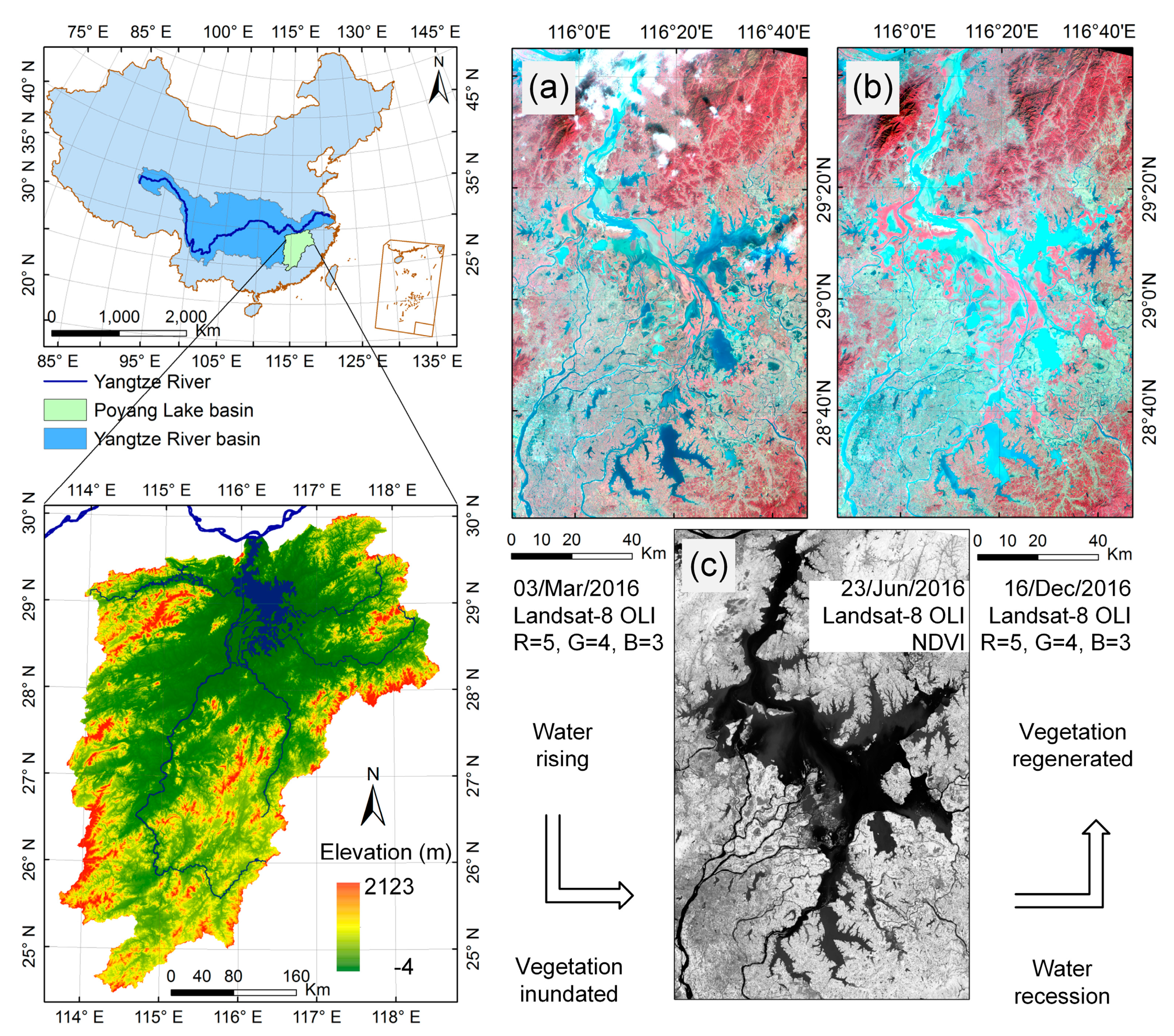
Poyang Lake (28°22′–29°45′N, 115°47′–116°45′E) is the largest freshwater lake in China and is well known for its ecological significance [53]. The lake receives water from five major river systems within the lake basin and discharges into the Yangtze River through its north outlet (Figure 1). Belonging to a humid subtropical climate zone, the annual precipitation in this lake basin is 1635.9 mm, and the annual mean surface air temperature was 17.5 °C for 1960–2010. Heavy rainfalls produce great surface discharges to the lake during the wet season from April–June. Rainfall declines sharply from July–September and remains relatively low from October–March. Jointly controlled by river discharges and interactions with the Yangtze River, the lake’s inundation area experiences significant seasonal variations, with large areas occurring in wet seasons and small areas in dry seasons. Water surface area can vary from less than 1000 km2 in winter during the dry season to over 3000 km2 in summer during the wet season. The climate condition benefits vegetation development in this shallow lake [54]. As a result, a unique lake-vegetation system exists (Figure 1), posing a challenge for accurate lake surface mapping.
2.2. MODIS NDVI MinVC Algorithm
2.2.1. Using the Minimum NDVI to Highlight Water Surfaces
Water bodies generally have negative NDVI values. Although the negative values vary as a result of differences in water turbidity and other mixtures, NDVI is an effective indicator of water bodies [6,36,44,48,49,55,56,57]. In contrast, vegetation generally has positive NDVI values. The contrasting NDVI behaviors form the basis for vegetation–water separation in the lake-vegetation system. Clouds are common in humid areas, especially in wet seasons. In the VNIR bands, spectral responses of thick clouds are generally flat, corresponding to NDVI values approaching zero. Attenuated by thin clouds, signals reflected from the underlying surfaces are blurred and the contrast of the NDVI image is reduced. Specifically, the NDVI value decreases over vegetation and increases over water bodies. Given the close-to-zero cloud NDVI values, the sign of NDVI values will be kept for cloud contaminated water and vegetation pixels.
Built-up areas, shadows, and snow may not have a large impact on water surface mapping in the Poyang Lake area. Within the lake area, almost no pixels show spectral features of artificial structures at the 250-m spatial scale due to sporadic villages and dense vegetation cover. The effects of shadows and snow can also be neglected in this flat and low-latitude area. Therefore, MODIS images consist mainly of water bodies, vegetation, and clouds (thick and thin) over the lake area. The exceptions may include some mudflat and sand banks [11,53] during the water recession period when vegetation has not yet regenerated. With an intermediate NDVI value between thick clouds and water bodies, these wet elements might be mistaken as water bodies by using image segmentation methods [58]. Despite this, the NDVI minima more likely correspond to a water pixel because water bodies always have lower NDVI values. Except for consecutive days of thick clouds, cloud free NDVI images can be generated by using the Minimum Value Composite (MinVC) algorithm (Table 1). In wet seasons with more cloudy days, a longer compositing period might increase the possibility of generating totally cloud free NDVI. The effects of cloud shadow are similar to cloud effects and can also be reduced by the MinVC algorithm.
2.2.2. MODIS Observations and the 16-day NDVI Product
MODIS is the key instrument onboard Terra and Aqua satellites that have operated successfully since their launches in December 1999 and May 2002. The complementary a.m. and p.m. satellites provide twice-daily global daytime observations at 250-m, 500-m, and 1-km resolutions. MODIS data in the VNIR bands have been well calibrated, corrected for atmospheric effects, and released as 250-m surface (SUR) reflectance products (Terra: MOD09Q1 and Aqua: MYD09Q1, the latest Collection 061 version used in this study, hereinafter referred to as MOD09). NDVI data are calculated by using the red band (620–670 nm) and the near-infrared band (841–876 nm) reflectance data, and composited into a 16-day product with the CV-MVC algorithm [59]. The product is released as MOD13Q1 (Terra) and MYD13Q1 (Aqua), intended to highlight vegetation information. In each year, MOD13Q1 starts from DOY001–353 (DOY means Day of Year), and MYD13Q1 from DOY008–361. A combination of MOD13Q1 and MYD13Q1 produces an equivalent 8-day NDVI dataset (hereinafter referred to as MOD13). In this study, all MOD13 data (the latest Collection 006 version) were used as of 2017. The dataset has masked out some water bodies by assigning a defaulted NDVI value of −0.3.
2.2.3. Generating the MinVC NDVI Data
Daily NDVI data were first calculated by using the 250-m MOD09Q1 (2000–2017) and MYD09Q1 (2002–2017) surface reflectance data in the red band (620–670 nm) and the near-infrared band (841–876 nm). Then, the pixelwise minimum NDVI values were determined by using the combined Terra and Aqua MODIS NDVI data within a 15-day moving window. The 15-day compositing period inherited all advantages of the 16-day compositing period used to produce the MOD13 NDVI product. The odd number meant the same days (i.e., one week) before and after a target day. More specifically, the ith-day MinVC NDVI image was created by using the daily MODIS NDVI images within the day i-7 and day i+7. Before the Aqua era, note that only Terra data were used. Different from the MODIS NDVI CV-MVC algorithm, this algorithm generated temporally continuous NDVI data. For example, the composite data at DOY1, 2010, also made use of MODIS NDVI data from DOY359–365, 2009.
In addition to the baseline algorithm, MinVC NDVI variants were generated by using a different compositing period or data source. First, a shorter 7-day moving window was used. The 15-day and 7-day periods were compared with respect to their performances on cloud removal. Second, the top-of-atmosphere (TOA), instead of SUR reflectance, was used. In this case, the MOD02QKM (Terra) and MYD02QKM (Aqua) products (the latest Collection 061 version) were used. The data were initially calibrated to TOA reflectance, and then followed the processing steps for SUR reflectance data. The two data sources were compared to investigate atmospheric effects on the MinVC NDVI data. In sum, the MinVC NDVI data had four variants, including the 15-day SUR reflectance based (baseline), the 7-day SUR reflectance based, the 15-day TOA reflectance based, and the 7-day TOA reflectance based. In this study, we focused on the baseline MinVC NDVI data, because the MOD13 NDVI product was generated by using SUR reflectance data with a similar compositing period.
2.3. Water Surface Mapping
An active contour model (“snake detector”) was used to segment the daily MinVC NDVI images. Active contour models are developed within the framework of energy minimization. Generally, these models include an energy function and a terminal function [60]. The energy function is composed of two parts, an internal one to control the smoothness of the curve (evolving boundary) and an external one to attract the curve towards the desired boundary. The external energy can be provided by but not limited to the image gradient. Chen and Vese [61] propose an active contour model based on the Mumford–Shah segmentation technique and the level-set method. The model has an energy function
where C is the evolving boundary, L is the length of C, inside(C) and outside(C) are the areas inside and outside C, with mean image values of c1 and c2, and u0 is the image value at coordinate (x, y). Minimizing Equation (1) generates the desired boundary C0.
The model does not necessarily depend on image gradient, works well for noisy images, and is less dependent on the position of initial conditions [61]. These features are positive for water surface mapping over shallow lakes, for example, the Poyang Lake. First, these lakes possess varying degrees of water turbidity, especially near river estuaries. The heterogeneous and noisy lake surfaces can be discerned by using this model. Second, the lake bottomland is topographically complicated, and the transition between water and land phases is frequent as a result of hydrological variability in the Poyang Lake. The model can deal with such topological changes in the lake surface by using identical initial conditions. In this study, the model was applied to the daily MinVC NDVI and the MOD13 NDVI. To implement the model, 40×40 uniformly distributed circles at a radius of 1.5 km were used as initial conditions. These processing steps were completed on the MATLAB R2015a (MathWorks Inc.) platform.
2.4. Water Surface Data Comparison and Validation
Water surface area data derived from MinVC NDVI were comprehensively evaluated. First, the composting algorithms were evaluated for their effectiveness to highlight water surface information (7-day vs. 15-day; SUR vs. TOA reflectance) (see Section 3.1). Second, the MinVC NDVI based result was validated by reference to the 30-m Landsat based result (NDWI threshold method), which was used as ground truth (see Figure 5 in Section 3.2). Within an image area including a land-water boundary, the NDWI histogram was analyzed to determine a single threshold value for land-water separation. Third, the MinVC NDVI based result was compared to the daily MIKE21 hydrodynamic modeling result [62,63,64,65] (see Figure 6 in Section 3.2). To drive the MIKE21 model, runoff data were obtained from gauged stations, and runoffs from the ungauged area were calculated by using a linear extrapolation of the gauged runoffs [63]. The total runoffs were specified as the upstream boundary conditions at the outlets of the five catchments (defined by the five major rivers in Figure 1). Daily water stages at the Hukou hydrological station (near the lake outlet) were used to define the downstream boundary condition. Values of other parameters followed those used in [64]. Due to the limitation of input data, the model was only implemented from 2000–2012. For hydrodynamic simulation, the whole lake area was divided as 20450 triangular elements, ranging from 0.007–0.605 km2. Those elements with water depth >0.4 m were counted as inundated, and the areas of inundated elements were summed as total water surface area [64]. The modeling result has been validated by using gauged water stage and river runoff data [64] and has been recently used for investigating lake surface dynamics [65]. Fourth, the MinVC NDVI based result was compared to other MODIS based results, including the cloud free MODIS NDVI based result (using the NDVI based thresholding method), the MOD13 NDVI based result (using the same active contour model), and the 30-m Landsat-MOD13 NDVI fusion based result [37,66] (see Section 3.3). For all comparisons, the coefficient of determination (R2), root mean square error (RMSE), regression slope, and intercept were used as statistical metrics. To sum up, Table 2 shows the list of all water surface area data.
2.5. Calculation of Water Submersion Time and Trend in Water Surface Area
The spatial distribution and temporal evolution of water surfaces were analyzed by using the MinVC NDVI based water surface area data. In each year from 2000–2017, daily water masks were generated by assigning the value 1 for water surfaces and the value 0 for non-water surfaces. Spatially, the annual maps of water submersion time (or inundation frequency) were produced by averaging daily water surfaces within each year [38,42,53]. The values of water submersion time may vary from 0%–100%. The map of annual mean water submersion time (2000–2017) was calculated by averaging the 18-year maps. Temporally, time series water surface area data were presented, and the temporal trends were calculated. The differences among multiple water surface area data and the potential causal factors were investigated. To sum up, Figure 2 shows the flowchart of this study.
3. Results
3.1. MinVC NDVI Performance on Highlighting Water Surfaces
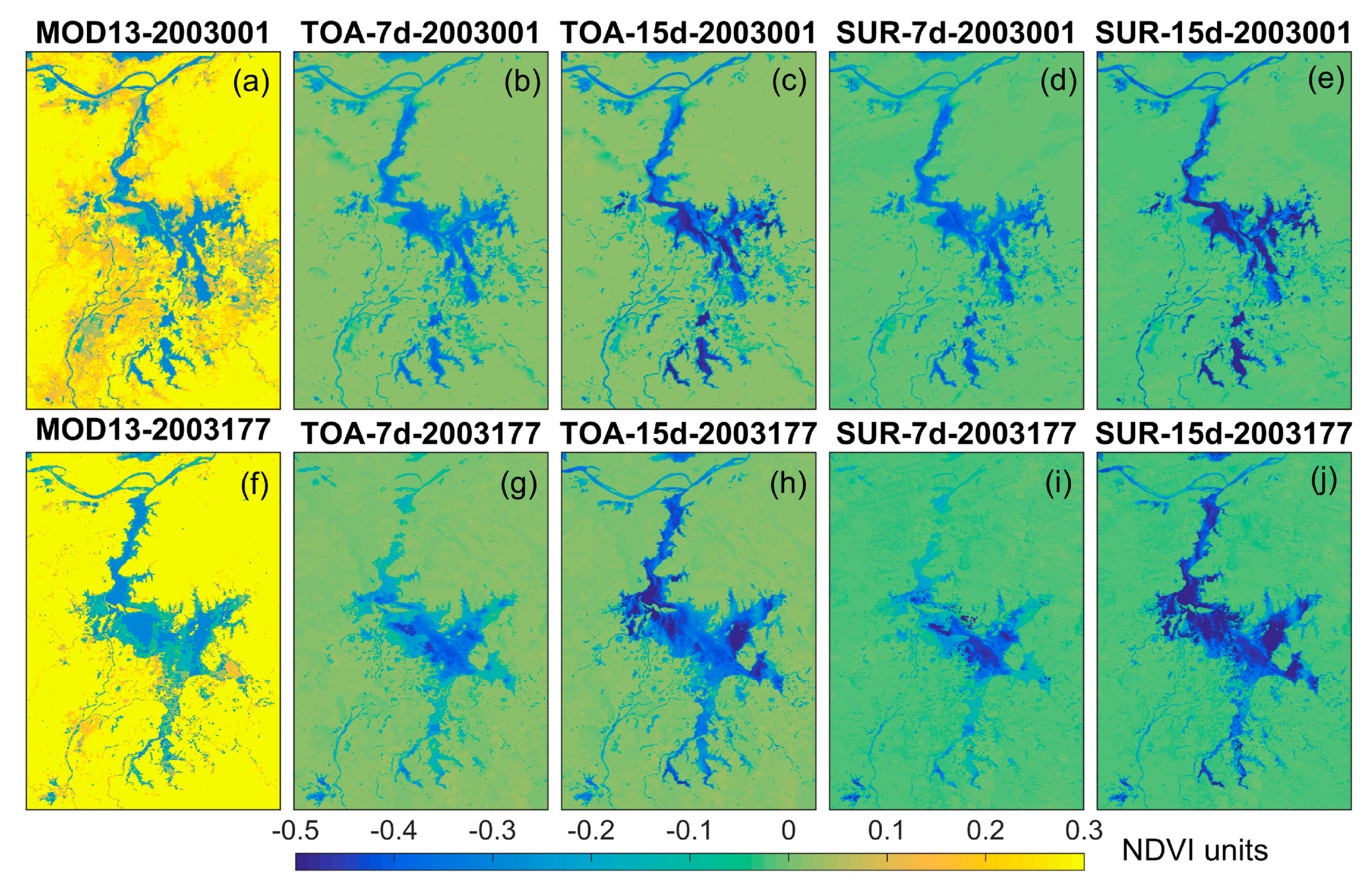
The MinVC NDVI highlighted water surfaces by suppressing cloud effects. Figure 3 shows MOD13 NDVI and four MinVC NDVI composites (7-day and 15-day; TOA and SUR) in DOY001, 2003 (dry season) and DOY177, 2003 (wet season). MOD13 NDVI showed more details on vegetation distribution over land in both seasons. Over water surfaces, some pixels were assigned the defaulted NDVI value (–0.3) and others even showed a typical vegetation spectral feature (Figure 3a,f), which might have an impact on water surface mapping. By contrast, the four NDVI composites had close-to-zero values over land and negative values over water. Both land and water areas had spatially homogenous NDVI values. The 15-day MinVC NDVI had more negative NDVI values and exhibited water surfaces than the 7-day MinVC NDVI. The latter might still be obscured by clouds, especially in wet seasons (Figure 3g,i). By using more than doubled MODIS images, the 15-day MinVC NDVI reduced the risk being affected by clouds. No marked differences were observed between the TOA and SUR reflectance based NDVI composites, except that the latter had overall lower values. As expected, large negative NDVI values were observed occasionally for the latter due to inaccurate atmospheric correction.
The compositing period and data source had an impact on water surface mapping results. Figure 4 shows concurrent MODIS NDVI and four MinVC NDVI composites at DOY175, 2016, (wet season) and DOY351, 2016 (dry season), when cloud free Landsat images are available within the composting period (indicating the availability of cloud free MODIS images). With at least one cloud free MODIS image, the 7-day and 15-day NDVI composites generated similar lake surface area data in the wet season. The conclusion was true for both the TOA reflectance based and the SUR reflectance based NDVI composites. In the dry season, the 15-day MinVC NDVI generated larger water surface area data than the 7-day counterpart. Compared to the Landsat based result, the baseline algorithm (15-day SUR reflectance) might underestimate water surface areas in wet seasons and perform better in dry seasons. In addition, the cloud free MODIS NDVI based result also underestimated lake surface areas relative to the Landsat based result, which might be due to scaling issues. It seemed that TOA NDVI outperformed SUR NDVI for lake surface mapping, especially in wet seasons.
3.2. Accuracy of MinVC NDVI Based Water Surface Area Data
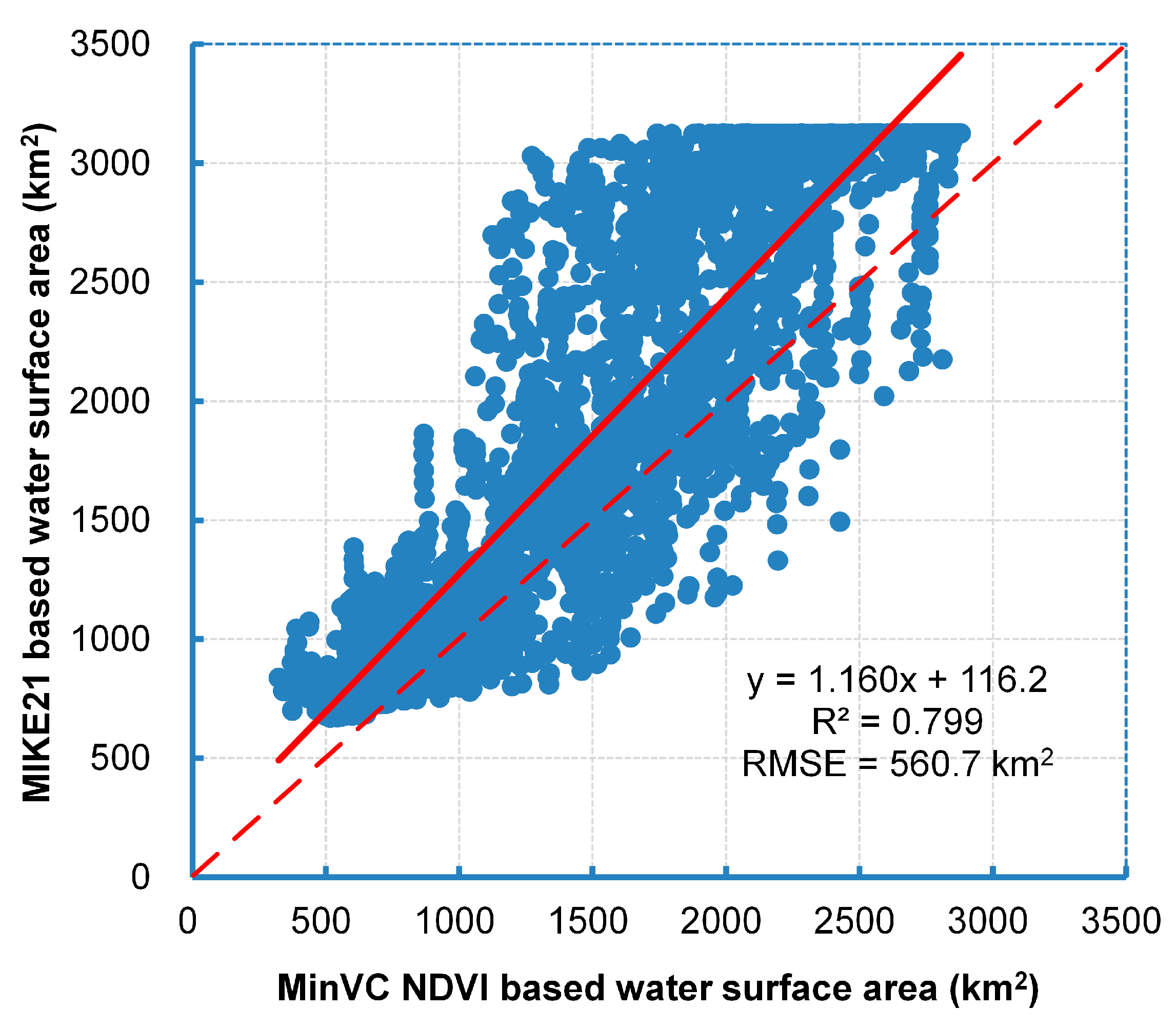
The baseline MinVC NDVI based water surface area data were in good agreement with both the 30-m Landsat based result (R2 = 0.914, Figure 5) and the daily hydrodynamic modeling result (R2 = 0.799, Figure 6). The former elucidated the absolute accuracy (RMSE = 223.7 km2) and the latter elucidated the temporal consistency of the derived water surface area data. Our result might underestimate water surface area in wet seasons (corresponding to large water surfaces in Figure 5) and slightly overestimate water surface area in dry seasons (corresponding to small water surfaces in Figure 5). The MIKE21 hydrodynamic model had known artifacts (e.g., coarse grid size; topography data not updated) in modeling water regimes over topographically flat lake bottoms (e.g., small lakes in the western lake areas). These were part of the reasons why large discrepancies were observed between the MinVC NDVI based and the MIKE21 based water surface area data (RMSE = 560.7 km2, Figure 6).
3.3. Performance of MODIS Based Water Surface Area Data
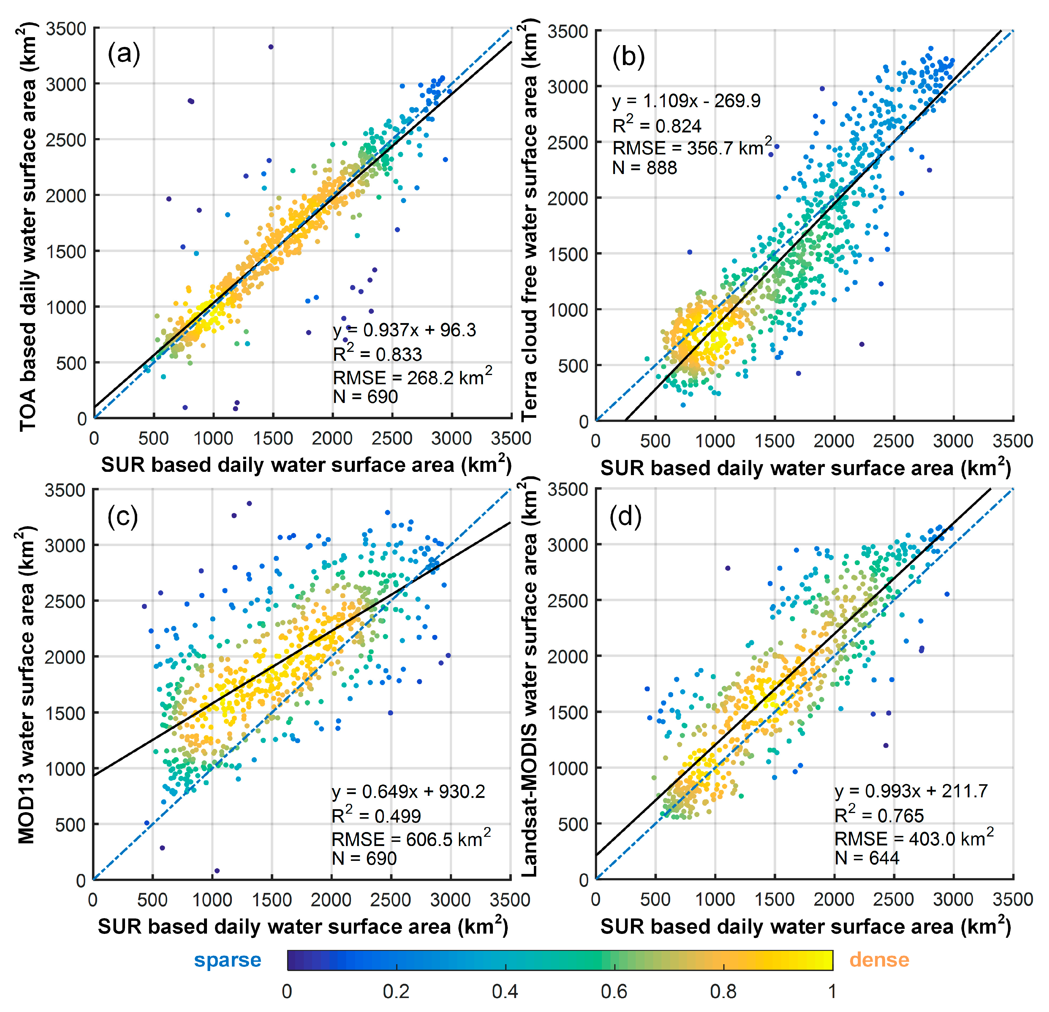
The baseline MinVC NDVI based water surface area data were comparable to other MODIS based results (Figure 7). As previously illustrated in Figure 4, the SUR reflectance based MinVC NDVI might generate smaller water surface area data than the TOA reflectance based MinVC NDVI, especially in wet seasons (Figure 7a). Despite this, the two results were in good agreement with each other (R2 = 0.833). Compared to the cloud free MODIS NDVI based result, our result might overestimate water surface areas in dry seasons and underestimate water surface areas in wet seasons (Figure 7b). The two results were also highly consistent with each other (R2 = 0.824). For NDVI composite product, MOD13 NDVI generated overall larger water surface area data relative to the MinVC NDVI, especially for small water surfaces (Figure 7c). Integrated with information from Landsat data, the MOD13 NDVI was more powerful in water surface delineation. As a result, the Landsat-MOD13 NDVI generated a more consistent result with the MinVC NDVI (Figure 7d). The former had a systematical positive bias value of ~211.7 km2, and the regression slope value was very close to 1.
The baseline MinVC NDVI based result might overestimate water surface areas in dry seasons, in particular in rapid water surface expansion and recession periods. A comparison of the MinVC NDVI based and the cloud free MODIS NDVI based results (Figure 8) showed that positive differences (MinVC relative to cloud free) were large (up to 400 km2) in March and April (normally corresponding to rapid water surface expansion period) and in October and November (normally corresponding to rapid water surface recession period). Negative differences were observed in June–August, which might be caused by incomplete cloud removal due to permanent cloud coverage in wet seasons.
3.4. Spatial Patterns of Lake Water Surface
The baseline MinVC NDVI based result provided temporally continuous water surface area data, based on which the evolution of the flood/drought event can be investigated. Figure 9 illustrates monthly water surface distribution for the Poyang Lake in 2010, a known typical flooding year. In April, the lake surface expanded rapidly to a large area and stayed until the end of September. The long-lasting large water surfaces made the year 2010 as the most severe flooding year in the recent decade. It is well known that transitions between flooding and drought events are common in the Poyang Lake. Figure 10 illustrates monthly water surface distribution in the next year, the most severe drought year in the recent decade. The lake surface remained at a small area until the end of May. With a relatively large area in June (still smaller than the lake area in June 2010), the water surface began to shrink until the end of year. During the drought year, the small isolated lakes in the western lake area were almost dried, which might have caused significant ecological consequences. In contrast, these lakes can be observed during the flooding year, especially from October–December, 2010 (Figure 9). An average of these daily water surface maps corresponded to an overall description of water submersion time in the Poyang Lake (Figure 11).
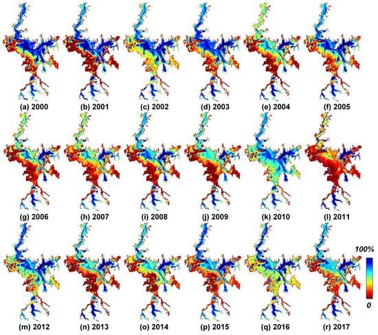
Dry and wet years were determined from the annual maps of water submersion time (Figure 12). The most severe drought event in 2011 was characterized by extremely short water submersion time all over the lake area except for some isolated reservoirs (Figure 12l). The known drought events in 2006 and 2013 were also manifested on the water submersion maps (Figure 12g,n), yet with lesser strength. Jointly controlled by meteorological (e.g., precipitation) and hydrological (inflow and outflow) conditions, smaller water surfaces may occur in some but not all months. Therefore, the maps might not show a markedly short water submersion time (e.g., 2006). Nevertheless, the wet years (2010, 2012, and 2016) were generally associated with long submersion time (Figure 12k,m,q). It seemed that the 2010 flooding event was the most severe in the recent decade, followed by the 2016 and the 2012 flooding events. Note that the results in 2000–2002 were less reliable because Aqua MODIS images were not included for NDVI compositing until July 2002. Similar results have been reported in [38,67,68].
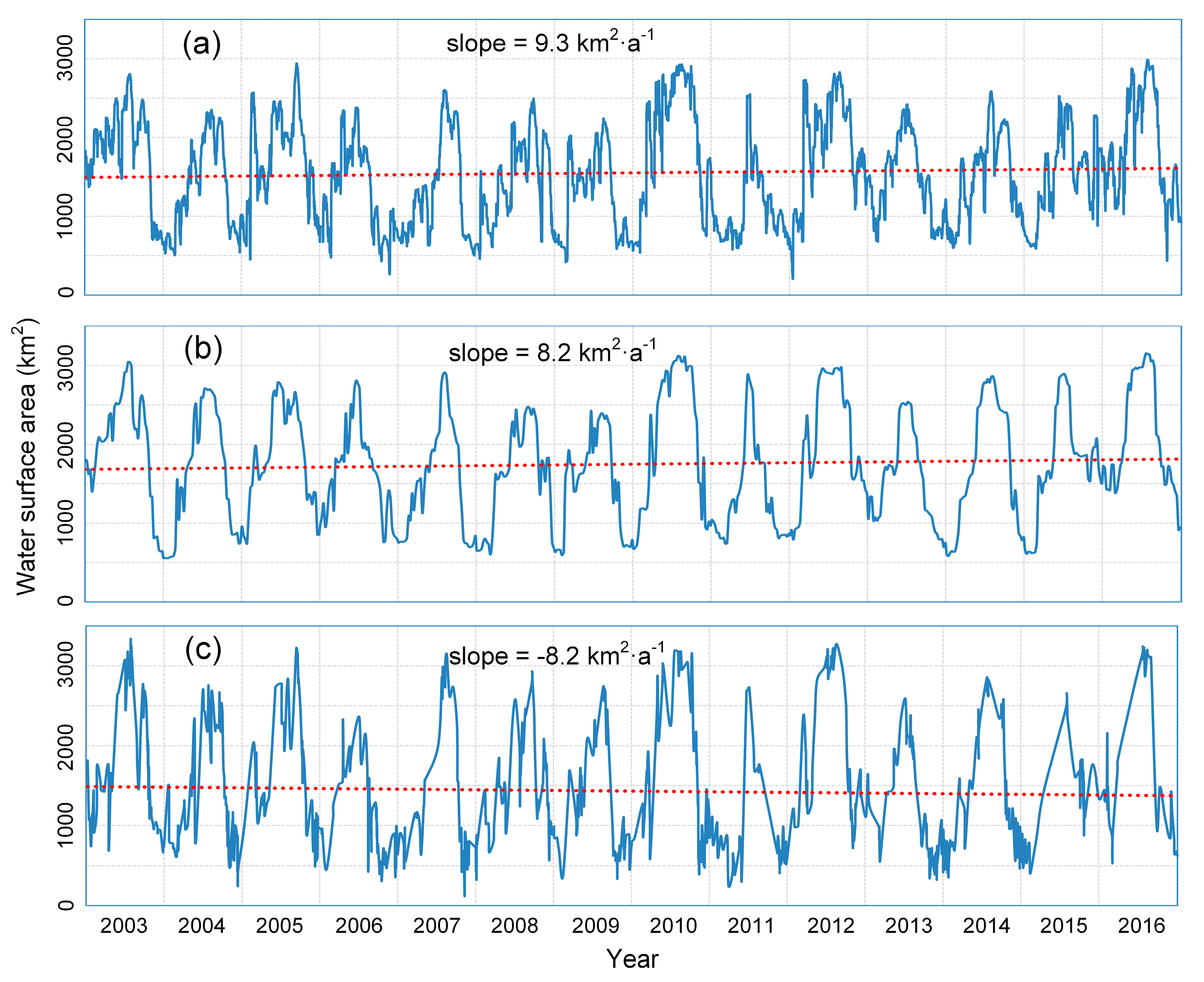
3.5. Temporal Variations in Lake Water Surface Area
Temporally continuous NDVI generated opposite trends in water surface area to the unevenly distributed cloud free NDVI. Within a common period in 2003–2016, water surface area increased by 9.3 km2·a−1 as derived using the MODIS MinVC NDVI (daily resolution), and increased by 8.2 km2·a−1 as derived using the Landsat-MOD13 NDVI (8-day resolution) (Figure 13). Large water surfaces in the recent wet years (2010, 2012, and 2016) might have reversed the declining trends in water surface area during the early 2000s. In contrast, the cloud free NDVI still revealed a declining trend at a rate of 8.2 km2·a−1. The uneven temporal distribution of cloud free MODIS images, more in dry seasons and less in wet seasons (Figure 14a), might account for the opposite trends. Although long-lasting large water surfaces might have occurred in recent wet years, the number of totally cloud free images decreased as a result of continuous cloudy and rainy days. Figure 14b shows that the cloud free NDVI based water surface area data followed a Gumbel distribution (R2 = 0.919) with a most likely water surface area of 865.5 km2.
4. Discussion
4.1. Added Value of the MinVC NDVI for Water Surface Mapping
Cloudy and rainy days lead to less cloud free images in wet seasons when water surfaces are, in the meantime, undergoing rapid expansion. High frequency lake surface data are needed in response to this contradiction. In addition, temporally continuous data are required to generate a reliable trend in water surface area. Fortunately, SAR images (e.g., Sentinel-1 at a 10-m resolution) are now capable of high frequency and high-resolution water surface mapping, although limited data are available for tracking long-term water surface area changes (e.g., dating back to 1980s) compared to optical remote sensing data. The passive microwave radiometers and geostationary sensors offer candidate data for all-sky or high frequency water surface monitoring; however, their spatial resolutions are insufficient for most inland water bodies [3,50]. MODIS sensors onboard Terra and Aqua satellites well balance the requirements of spatial and temporal resolutions, and play an important role in water surface mapping. There is a general tendency to exploit the entire MODIS data archive, from both Terra and Aqua, for added information in change detection studies [49,51]. These data are important for tracking rapidly changing natural processes at daily scales, including water surface changes. In this context, this study proposes a simple yet effective method for daily water surface mapping.
The NDVI MinVC algorithm suppresses cloud effects by using complementary cloud free or thin cloud covered information on bi-monthly Terra and Aqua MODIS images. There are at least 30 Terra and Aqua MODIS images within the 15-day moving window, and the number increases toward high-latitude regions, increasing the probability to generate totally cloud free NDVI images. In addition to cloud removal, the algorithm can deal with other issues that complicate water surface mapping. Two of them are sun glint and water turbidity, both leading to increased NDVI values of water pixels. Generally caused by transient hydrological (e.g., large river runoff as a result of heavy rainfall) and meteorological (e.g., strong wind) events, these effects can be reduced by selecting the NDVI minima. The algorithm even improves the effective spatial resolution of water surface maps. Because MODIS is a whiskbroom scanner, the 250-m resolution in nadir-viewing direction can be reduced to over 1-km across track and 500-m along track. Fortunately, our algorithm inclines to select nadir-viewing water pixels instead of land-water mixed pixels that generally have larger NDVI values.
4.2. Causes of Differences among Multiple Lake Surface Data
The 30-m Landsat images can accurately delineate water surfaces at the days of image acquisition. At a 250-m resolution, the cloud free MODIS NDVI generates high frequency (relative to Landsat, ~6-day effective temporal interval, unevenly distributed) lake surface information. Concurrent daily Terra and Aqua images further corroborate the derived water surface area data, which serve as a solid basis for algorithm validation. By reference to the cloud free NDVI, the MinVC NDVI overestimates water surface areas for small lake surfaces and underestimates water surface areas for large lake surfaces. By selecting minimum NDVI values, the NDVI MinVC algorithm is inclined to include more wet pixels in dry seasons. Generally, multiple scenes of cloud free or thin cloud covered images are available in dry seasons. The algorithm tends to reserve more pixels in the second half of the compositing period (if any) at the water rising stage, while reserving more pixels in the first half of the composition period (if any) at the water recession stage. This situation is more serious at rapid water rising and recession stages. Although lake surface areas tend to be overestimated in the transitional periods, the temporal pattern might be kept by using the NDVI MinVC algorithm. In this circumstance, the 15-day moving window functions like a filter that selects the maximum value in the 15-day compositing period. Because of the 15-day compositing period, the maximum phase difference between our result and the actual lake surface change can be one week in advance (having cloud free image with the largest lake surface) or one week lagging behind (having cloud free image with the smallest lake surface). The accurate phase difference, however, varies depending on the availability of cloud free MODIS images. Meanwhile, the occurrence of wet sand and mudflat (both showing negative NDVI values) can be confused with water surfaces at the water recession stage when vegetation has not yet regenerated. In wet seasons, however, residual cloud effects might contribute to the underestimation of lake surface areas. Given the good consistency between the MinVC NDVI based and the Landsat-MOD13 NDVI based results (Figure 7d and Figure 13a,b), the issues of overestimation and underestimation are likely shared by image compositing based methods.
Various factors may determine the differences among multiple water surface area data. Intended to highlight vegetation information, the MOD13 NDVI seems to reduce NDVI contrast over the lake area. Therefore, it generates overall larger lake surface areas compared to the MinVC NDVI by using the same active contour model. Nevertheless, the Landsat-MOD13 fusion technique decomposes the original MOD13 NDVI using the Landsat NDVI, which largely improves the ability of MOD13 NDVI for water surface mapping. The MIKE21 model also generates overall larger water surface areas than the MinVC NDVI. Tan et al. [37] showed the poor performance of MIKE21 to model water inundation in topographically flat lake areas. Zhang et al. [65] also found that the modeling results overestimated water surface areas that were determined from cloud free MODIS images, which is in agreement with our conclusion. The differences might also be caused by topographical changes in the Poyang Lake. Topography data collected in 1998 were used to drive the model, which cannot reveal the effects of changing topography on lake surface areas in recent decades [62]. Specifically, sand mining near the north lake outlet has been reported to increase the lake’s discharge to the Yangtze River and probably caused the decline in lake surface areas, particularly in dry seasons [69].
4.3. Improvements of Current NDVI MinVC Algorithm
Long compositing period (i.e., 15-day) has an impact on water surface mapping. Currently, the baseline algorithm uses no prior knowledge and assumes a relaxed uniform compositing period. The main objective is to derive cloud free NDVI images in wet seasons as much as possible. However, the treatment also exacerbates the situation of lake surface area overestimation in dry seasons. To reduce such effects, MODIS cloud mask data can be used to determine time-varying compositing periods. It is safe to assume that the compositing period is inversely proportional to the overall cloud amount. More specifically, no cloud coverage (totally cloud free) means a daily compositing period, and larger cloud amount corresponds to a longer compositing period. Because the mean temporal interval of cloud free MODIS images is ~six days, such time-varying compositing periods are reasonable and are expected to perform better than the fixed 15-day compositing period. With regard to data source, TOA instead of surface reflectance is recommended for NDVI MinVC composting, although minor differences are observed between results derived from the two composites.
A combination of multiple remote sensing data enhances the possibility of cloud free NDVI data. Within a day, satellite images acquired at a different time from Terra and Aqua MODIS images (10:30 and 13:30 Local Time) can provide complementary cloud free information. Such sensors include, but are not limited to, the ENVISAT MERIS (10:00 Local Time, 2002-2012), the Sentinel-3 OLCI (10:00 Local Time, 2016-present), and the NOAA/MetOp AVHRR (overpassing times varying dependent on orbital drift, 1970s-present). Prior to the MODIS era, the AVHRR data can be used alone to generate MinVC NDVI. Several contemporary a.m. and p.m. orbiting AVHRR sensors may overpass the earth surface at different times, especially when considering the orbital drift issues for earlier sensors. By applying the MinVC algorithm to those dense NDVI images, cloud effects can be further reduced. Due to different spectral response functions (relative spectral responses), however, the inter-sensor NDVI differences should be adjusted in advance before any compositing. In most cases, a linear equation is qualified for a reliable spectral adjustment [70,71,72]. Within the framework of NDVI intercalibration, moderate-resolution and high-resolution images can be combined for water surface mapping. Note that the proposed algorithm can be accommodated to other indices that are sensitive to water surfaces.
High-resolution satellite images are required for improved water surface mapping. The relevant sensors include the NASA Landsat series sensors, the ESA Sentinel-2 Multispectral Imager (MSI), and the Chinese HJ/GF series sensors. These sensors data can be employed in at least two aspects. First, a synergy of high-resolution images (e.g., Landsat-8 OLI and Sentinel-2 MSI as in [73,74]) provide an improved reference dataset for validation purposes. Second, high-resolution satellite images can be integrated with the MinVC NDVI to derive long-term high-resolution water surface area data (e.g., [36,37]). These data are expected to benefit monitoring small lakes with an area even in the order of several MODIS pixels [66].
5. Conclusions
This study proposed a simple MODIS NDVI based MinVC algorithm to generate daily water surface area data over seasonally flooded wetlands by using the combined daily 250-m Terra and Aqua MODIS NDVI images. The baseline algorithm first created daily Minimum Value Composite NDVI by selecting pixelwise NDVI minima within a 15-day moving window. Consisting mainly of water pixels over water and cloud pixels over land, the daily MinVC NDVI data were then segmented for water surfaces from the cloud background. The derived water surface result compared well with the Landsat based, the cloud free MODIS image based, the hydrodynamic modeling based, and the Landat-MOD13 image fusion based results, and outperformed the MOD13 NDVI based result. Our result provided high frequency and reliable descriptions of water surface dynamics in both space and time. The proposed algorithm has the potential to make full use of fragmented cloud free information from the entire MODIS VNIR data archive for water surface mapping of seasonally flooded wetlands. Within the framework of satellite intercalibration, the algorithm can integrate multiple satellite senor data, both moderate-resolution and high-resolution, for improved water surface mapping.
Author Contributions
Conceptualization, X.F. and Y.L.; methodology, X.F.; validation, G.W. and X.Z.; writing—original draft preparation, X.F.; writing—review and editing, Y.L. All authors have read and agree to the published version of the manuscript.
Funding
This study was funded by the National Natural Science Foundation of China (NSFC), grant number. 41701414.
Acknowledgments
The MODIS data were collected from the Level-1 and Atmosphere Archive and Distribution System (LAADS) Distributed Active Archive Center (DAAC), Goddard Space Flight Center (GSFC). The original results of hydrodynamic modeling were kindly provided by Dr. Zhiqiang Tan. The authors would like to thank the anonymous reviewers for their constructive comments. Their expertise in remote sensing and knowledge on the Poyang Lake largely improves this study.
Conflicts of Interest
The authors declare no conflict of interest.
References
- McFeeters, S.K. The use of the Normalized Difference Water Index (NDWI) in the delineation of open water features. Int. J. Remote Sens. 1996, 17, 1425–1432. [Google Scholar] [CrossRef]
- Shcherbenko, Y.V.; Doroshenko, S.G. Monitoring high-water conditions using nighttime thermal imagery. Mapp. Sci. Remote Sens. 2002, 39, 170–180. [Google Scholar] [CrossRef]
- De Groeve, T. Flood monitoring and mapping using passive microwave remote sensing in Namibia. Geomat. Nat. Haz. Risk 2010, 1, 19–35. [Google Scholar] [CrossRef]
- Malinowski, R.; Hofle, B.; Koenig, K.; Groom, G.; Schwanghart, W.; Heckrath, G. Local-scale flood mapping on vegetated floodplains from radiometrically calibrated airborne LiDAR data. ISPRS J. Photogramm. 2016, 119, 267–279. [Google Scholar] [CrossRef]
- Du, J.; Kimball, J.S.; Galantowicz, J.; Kim, S.-B.; Chan, S.K.; Reichle, R.; Jones, L.A.; Watts, J.D. Assessing global surface water inundation dynamics using combined satellite information from SMAP, AMSR2 and Landsat. Remote Sens. Environ. 2018, 213, 1–17. [Google Scholar] [CrossRef]
- Ma, M.; Wang, X.; Veroustraete, F.; Dong, L. Change in area of Ebinur Lake during the 1998–2005 period. Int. J. Remote Sens. 2007, 28, 5523–5533. [Google Scholar] [CrossRef]
- Jain, S.K.; Singh, R.D.; Jain, M.K.; Lohani, A.K. Delineation of flood-prone areas using remote sensing techniques. Water Resour. Manag. 2005, 19, 333–347. [Google Scholar] [CrossRef]
- Xu, H.Q. Modification of Normalised Difference Water Index (NDWI) to enhance open water features in remotely sensed imagery. Int. J. Remote Sens. 2006, 27, 3025–3033. [Google Scholar] [CrossRef]
- Feyisa, G.L.; Meilby, H.; Fensholt, R.; Proud, S.R. Automated water extraction index: A new technique for surface water mapping using Landsat imagery. Remote Sens. Environ. 2014, 140, 23–35. [Google Scholar] [CrossRef]
- Ticehurst, C.; Guerschman, J.P.; Chen, Y. The strengths and limitations in using the daily MODIS open water likelihood algorithm for identifying flood events. Remote Sens. 2014, 6, 11791–11809. [Google Scholar] [CrossRef] [Green Version]
- Dronova, I.; Gong, P.; Wang, L. Object-based analysis and change detection of major wetland cover types and their classification uncertainty during the low water period at Poyang Lake, China. Remote Sens. Environ. 2011, 115, 3220–3236. [Google Scholar] [CrossRef]
- Li, J.L.; Sheng, Y.W. An automated scheme for glacial lake dynamics mapping using Landsat imagery and digital elevation models: A case study in the Himalayas. Int. J. Remote Sens. 2012, 33, 5194–5213. [Google Scholar] [CrossRef]
- Yang, K.; Smith, L.C. Supraglacial streams on the Greenland ice sheet delineated from combined spectral-shape information in high-resolution satellite imagery. IEEE Geosci. Remote Sens. Lett. 2013, 10, 801–805. [Google Scholar] [CrossRef]
- Eilander, D.; Annor, F.O.; Iannini, L.; van de Giesen, N. Remotely sensed monitoring of small reservoir dynamics: A Bayesian approach. Remote Sens. 2014, 6, 1191–1210. [Google Scholar] [CrossRef] [Green Version]
- Wolski, P.; Murray-Hudso, M.; Thito, K.; Cassidy, L. Keeping it simple: Monitoring flood extent in large data-poor wetlands using MODIS SWIR data. Int. J. Appl. Earth Obs. 2017, 57, 224–234. [Google Scholar] [CrossRef] [Green Version]
- Hui, F.M.; Xu, B.; Huang, H.B.; Yu, Q.; Gong, P. Modelling spatial-temporal change of Poyang Lake using multitemporal Landsat imagery. Int. J. Remote Sens. 2008, 29, 5767–5784. [Google Scholar] [CrossRef]
- Soti, V.; Tran, A.; Bailly, J.S.; Puech, C.; Lo Seen, D.; Bégué, A. Assessing optical earth observation systems for mapping and monitoring temporary ponds in arid areas. Int. J. Appl. Earth Obs. 2009, 11, 344–351. [Google Scholar] [CrossRef] [Green Version]
- Zhao, X.; Stein, A.; Chen, X.L. Monitoring the dynamics of wetland inundation by random sets on multi-temporal images. Remote Sens. Environ. 2011, 115, 2390–2401. [Google Scholar] [CrossRef]
- Murray, N.J.; Phinn, S.R.; Clemens, R.S.; Roelfsema, C.M.; Fuller, R.A. Continental scale mapping of tidal flats across east Asia using the Landsat archive. Remote Sens. 2012, 4, 3417–3426. [Google Scholar] [CrossRef] [Green Version]
- Li, W.B.; Du, Z.Q.; Ling, F.; Zhou, D.B.; Wang, H.L.; Gui, Y.M.; Sun, B.Y.; Zhang, X.M. A comparison of land surface water mapping using the Normalized Difference Water Index from TM, ETM+ and ALI. Remote Sens. 2013, 5, 5530–5549. [Google Scholar] [CrossRef] [Green Version]
- Tulbure, M.G.; Broich, M. Spatiotemporal dynamic of surface water bodies using Landsat time-series data from 1999 to 2011. ISPRS J. Photogramm. 2013, 79, 44–52. [Google Scholar] [CrossRef]
- Yang, Y.H.; Liu, Y.X.; Zhou, M.X.; Zhang, S.Y.; Zhan, W.F.; Sun, C.; Duan, Y.W. Landsat 8 OLI image based terrestrial water extraction from heterogeneous backgrounds using a reflectance homogenization approach. Remote Sens. Environ. 2015, 171, 14–32. [Google Scholar] [CrossRef]
- Sheng, Y.W.; Song, C.Q.; Wang, J.D.; Lyons, E.A.; Knox, B.R.; Cox, J.S.; Gao, F. Representative lake water extent mapping at continental scales using multi-temporal Landsat-8 imagery. Remote Sens. Environ. 2016, 185, 129–141. [Google Scholar] [CrossRef] [Green Version]
- Arvor, D.; Daher, F.R.; Briand, D.; Dufour, S.; Rollet, A.J.; Simões, M.; Ferraz, R.P. Monitoring thirty years of small water reservoirs proliferation in the southern Brazilian Amazon with Landsat time series. ISPRS J. Photogramm. 2018, 145, 225–237. [Google Scholar] [CrossRef]
- Jia, K.; Jiang, W.G.; Li, J.; Tang, Z.H. Spectral matching based on discrete particle swarm optimization: A new method for terrestrial water body extraction using multi-temporal Landsat 8 images. Remote Sens. Environ. 2018, 209, 1–18. [Google Scholar] [CrossRef]
- Lu, S.L.; Wu, B.F.; Yan, N.N.; Wang, H. Water body mapping method with HJ-1A/B satellite imagery. Int. J. Appl. Earth Obs. 2011, 13, 428–434. [Google Scholar] [CrossRef]
- Du, Y.; Zhang, Y.H.; Ling, F.; Wang, Q.M.; Li, W.B.; Li, X.D. Water bodies’ mapping from Sentinel-2 imagery with Modified Normalized Difference Water Index at 10-m spatial resolution produced by sharpening the SWIR band. Remote Sens. 2016, 8, 354. [Google Scholar] [CrossRef] [Green Version]
- Jain, S.K.; Saraf, A.K.; Goswami, A.; Ahmad, T. Flood inundation mapping using NOAA AVHRR data. Water Resour. Manag. 2006, 20, 949–959. [Google Scholar] [CrossRef]
- Sakamoto, T.; Van Nguyen, N.; Kotera, A.; Ohno, H.; Ishitsuka, N.; Yokozawa, M. Detecting temporal changes in the extent of annual flooding within the Cambodia and the Vietnamese Mekong Delta from MODIS time-series imagery. Remote Sens. Environ. 2007, 109, 295–313. [Google Scholar] [CrossRef]
- Yésou, Y.; Huber, C.; Lai, X.; Averty, S.; Li, J.; Daillet, S.; Bergé-Nguyen, M.; Chen, X.; Huang, S.; James, B.; et al. Nine years of water resources monitoring over the middle reaches of the Yangtze River, with ENVISAT, MODIS, Beijing-1 time series, Altimetric data and field measurements. Lakes Reserv. Res. Manag. 2011, 16, 231–247. [Google Scholar]
- Klein, I.; Dietz, A.J.; Gessner, U.; Galayeva, A.; Myrzakhmetov, A.; Kuenzer, C. Evaluation of seasonal water body extents in Central Asia over the past 27 years derived from medium-resolution remote sensing data. Int. J. Appl. Earth Obs. 2014, 26, 335–349. [Google Scholar] [CrossRef]
- d’Andrimont, R.; Defourny, P. Monitoring African water bodies from twice-daily MODIS observation. Gisci. Remote Sens. 2018, 55, 130–153. [Google Scholar] [CrossRef]
- Zhang, F.; Zhu, X.L.; Liu, D.S. Blending MODIS and Landsat images for urban flood mapping. Int. J. Remote Sens. 2014, 35, 3237–3253. [Google Scholar] [CrossRef]
- Wu, G.P.; Liu, Y.B. Downscaling surface water inundation from coarse data to fine-scale resolution: Methodology and accuracy assessment. Remote Sens. 2015, 7, 15989–16003. [Google Scholar] [CrossRef] [Green Version]
- Huang, C.; Chen, Y.; Zhang, S.Q.; Li, L.Y.; Shi, K.F.; Liu, R. Surface water mapping from Suomi NPP-VIIRS imagery at 30 m resolution via blending with Landsat data. Remote Sens. 2016, 8, 631. [Google Scholar] [CrossRef] [Green Version]
- Chen, B.; Chen, L.F.; Huang, B.; Michishita, R.; Xu, B. Dynamic monitoring of the Poyang Lake wetland by integrating Landsat and MODIS observations. ISPRS J. Photogramm. 2018, 139, 75–87. [Google Scholar] [CrossRef]
- Tan, Z.; Li, Y.; Xu, X.; Yao, J.; Zhang, Q. Mapping inundation dynamics in a heterogeneous floodplain: Insights from integrating observations and modeling approach. J. Hydrol. 2019, 572, 148–159. [Google Scholar] [CrossRef]
- Andreoli, R.; Li, J.; Yesou, H. Flood extent prediction from lake heights and water level estimation from flood extents using river gauges, elevation models and ENVISAT data. In Proceedings of the ENVISAT Symposium 2007, Montreux, Switzerland, 23–27 April 2007. [Google Scholar]
- Ding, X.; Li, X. Monitoring of the water-area variations of Lake Dongting in China with ENVISAT ASAR images. Int. J. Appl. Earth Obs. 2011, 13, 894–901. [Google Scholar] [CrossRef]
- Milne, T.; Tapley, I.J. Assessment of wetland ecosystems and flooding in the Tonle Sap Basin, Cambodia, using AIRSAR. In Proceedings of the 2004 IEEE International Geoscience and Remote Sensing Symposium, Alaska, AK, USA, 20–24 September 2004; pp. 1858–1861. [Google Scholar]
- Twele, A.; Cao, W.; Plank, S.; Martinis, S. Sentinel-1-based flood mapping: A fully automated processing chain. Int. J. Remote Sens. 2016, 37, 2990–3004. [Google Scholar] [CrossRef]
- Feng, L.; Hu, C.M.; Chen, X.L.; Cai, X.B.; Tian, L.Q.; Gan, W.X. Assessment of inundation changes of Poyang Lake using MODIS observations between 2000 and 2010. Remote Sens. Environ. 2012, 121, 80–92. [Google Scholar] [CrossRef]
- Wu, G.P.; Liu, Y.B. Capturing variations in inundation with satellite remote sensing in a morphologically complex, large lake. J. Hydrol. 2015, 523, 14–23. [Google Scholar] [CrossRef]
- Weiss, D.J.; Crabtree, R.L. Percent surface water estimation from MODIS BRDF 16-day image composites. Remote Sens. Environ. 2011, 115, 2035–2046. [Google Scholar] [CrossRef]
- Huang, S.F.; Li, J.G.; Xu, M. Water surface variations monitoring and flood hazard analysis in Dongting Lake area using long-term Terra/MODIS data time series. Nat. Hazards 2012, 62, 93–100. [Google Scholar] [CrossRef]
- Chen, Y.; Huang, C.; Ticehurst, C.; Merrin, L.; Thew, P. An evaluation of MODIS daily and 8-day composite products for floodplain and wetland inundation mapping. Wetlands 2013, 33, 823–835. [Google Scholar] [CrossRef]
- Ogilvie, A.; Belaud, G.; Delenne, C.; Bailly, J.S.; Bader, J.C.; Oleksiak, A.; Ferry, L.; Martin, D. Decadal monitoring of the Niger Inner Delta flood dynamics using MODIS optical data. J. Hydrol. 2015, 523, 368–383. [Google Scholar] [CrossRef] [Green Version]
- Ahamed, A.; Bolten, J.D. A MODIS-based automated flood monitoring system for southeast Asia. Int. J. Appl. Earth Obs. 2017, 61, 104–117. [Google Scholar] [CrossRef] [Green Version]
- Fayne, J.V.; Bolten, J.D.; Doyle, C.S.; Fuhrmann, S.; Rice, M.T.; Houser, P.R.; Lakshmi, V. Flood mapping in the lower Mekong River Basin using daily MODIS observations. Int. J. Remote Sens. 2017, 38, 1737–1757. [Google Scholar] [CrossRef]
- Proud, S.R.; Fensholt, R.; Rasmussen, L.V.; Sandholt, I. Rapid response flood detection using the MSG geostationary satellite. Int. J. Appl. Earth Obs. 2011, 13, 536–544. [Google Scholar] [CrossRef]
- Wang, Z.S.; Schaaf, C.B.; Sun, Q.S.; Shuai, Y.M.; Roman, M.O. Capturing rapid land surface dynamics with Collection V006 MODIS BRDF/NBAR/Albedo (MCD43) products. Remote Sens. Environ. 2018, 207, 50–64. [Google Scholar] [CrossRef]
- Klein, I.; Dietz, A.; Gessner, U.; Dech, S.; Kuenzer, C. Results of the Global WaterPack: A novel product to assess inland water body dynamics on a daily basis. Remote Sens. Lett. 2015, 6, 78–87. [Google Scholar] [CrossRef]
- Dronova, I.; Gong, P.; Wang, L.; Zhong, L.H. Mapping dynamic cover types in a large seasonally flooded wetland using extended principal component analysis and object-based classification. Remote Sens. Environ. 2015, 158, 193–206. [Google Scholar] [CrossRef]
- Fan, X.; Liu, Y.; Tao, J.; Wang, Y.; Zhou, H. MODIS detection of vegetation changes and investigation of causal factors in Poyang Lake basin, China for 2001–2015. Ecol. Indic. 2018, 91, 511–522. [Google Scholar] [CrossRef]
- Liu, Y.B.; Song, P.; Peng, J.; Ye, C. A physical explanation of the variation in threshold for delineating terrestrial water surfaces from multi-temporal images: Effects of radiometric correction. Int. J. Remote Sens. 2012, 33, 5862–5875. [Google Scholar] [CrossRef]
- Rokni, K.; Ahmad, A.; Selamat, A.; Hazini, S. Water feature extraction and change detection using multitemporal Landsat imagery. Remote Sens. 2014, 6, 4173–4189. [Google Scholar] [CrossRef] [Green Version]
- Feng, M.; Sexton, J.O.; Channan, S.; Townshend, J.R. A global, high-resolution (30-m) inland water body dataset for 2000: First results of a topographic-spectral classification algorithm. Int. J. Digit. Earth 2016, 9, 113–133. [Google Scholar] [CrossRef] [Green Version]
- Yamano, H.; Shimazaki, H.; Matsunaga, T.; Ishoda, A.; McClennen, C.; Yokoki, H.; Fujita, K.; Osawa, Y.; Kayanne, H. Evaluation of various satellite sensors for waterline extraction in a coral reef environment: Majuro Atoll, Marshall Islands. Geomorphology 2006, 3–4, 398–411. [Google Scholar] [CrossRef]
- Didan, K.; Munoz, A.B.; Solano, R.; Huete, A. MODIS Vegetation Index User’s Guide (MOD13 Series); Vegetation Index and Phenology Lab, University of Arizona: Tucson, AZ, USA, 2015. [Google Scholar]
- Kass, M.; Witkin, A.; Terzopoulos, D. Snakes: Active contour models. Int. J. Comput. Vis. 1988, 1, 321–331. [Google Scholar] [CrossRef]
- Chen, T.F.; Vese, L.A. Active contours without edges. IEEE Trans. Image Process. 2001, 10, 266–277. [Google Scholar] [CrossRef] [Green Version]
- Yao, J.; Zhang, Q.; Ye, X.; Zhang, D.; Bai, P. Quantifying the impact of bathymetric changes on the hydrological regimes in a large floodplain lake: Poyang Lake. J. Hydrol. 2018, 561, 711–723. [Google Scholar] [CrossRef]
- Zhang, Q.; Ye, X.C.; Werner, A.D.; Li, Y.L.; Yao, J.; Li, X.H.; Xu, C.Y. An investigation of enhanced recessions in Poyang Lake: Comparison of Yangtze River and local catchment impacts. J. Hydrol. 2014, 517, 425–434. [Google Scholar] [CrossRef] [Green Version]
- Tan, Z.Q.; Zhang, Q.; Li, M.F.; Li, Y.L.; Xu, X.L.; Jiang, J.H. A study of the relationship between wetland vegetation communities and water regimes using a combined remote sensing and hydraulic modeling approach. Hydrol. Res. 2016, 47, 278–292. [Google Scholar]
- Zhang, X.L.; Zhang, Q.; Werner, A.D.; Tan, Z.Q. Characteristics and causal factors of hysteresis in the hydrodynamics of a large floodplain system: Poyang Lake (China). J. Hydrol. 2017, 553, 574–583. [Google Scholar] [CrossRef] [Green Version]
- Tan, Z.; Wang, X.; Chen, B.; Liu, X.; Zhang, Q. Surface water connectivity of seasonal isolated lakes in a dynamic lake-floodplain system. J. Hydrol. 2019, 579, 124154. [Google Scholar] [CrossRef]
- Yesou, H.; Huber, C.; Haouet, S.; Lai, X.; Huang, S.; de Fraipont, P.; Desnos, Y.L. Exploiting sentinel 1 time series to monitor the largest fresh water bodies in PR China, the Poyang Lake. In Proceedings of the 2016 IEEE International Geoscience and Remote Sensing Symposium (IGARSS), Beijing, China, 10–15 July 2016; pp. 3882–3885. [Google Scholar]
- Sun, Y.; Huang, S.; Li, J.; Li, X.; Ma, J.; Wang, H.; Lei, T. Monitoring seasonal changes in the water surface areas of Poyang Lake using Cosmo-Skymed time series data in PR China. In Proceedings of the 2016 IEEE International Geoscience and Remote Sensing Symposium (IGARSS), Beijing, China, 10–15 July 2016; pp. 7180–7183. [Google Scholar]
- Lai, X.J.; Shankman, D.; Huber, C.; Yesou, H.; Huang, Q.; Jiang, J.H. Sand mining and increasing Poyang Lake’s discharge ability: A reassessment of causes for lake decline in China. J. Hydrol. 2014, 519, 1698–1706. [Google Scholar] [CrossRef]
- Fan, X.; Liu, Y. A global study of NDVI difference among moderate-resolution satellite sensors. ISPRS J. Photogramm. 2016, 121, 177–191. [Google Scholar] [CrossRef]
- Fan, X.; Liu, Y. Using a MODIS index to quantify MODIS-AVHRRs spectral differences in the visible band. Remote Sens. 2018, 10, 61. [Google Scholar] [CrossRef] [Green Version]
- Fan, X.; Liu, Y. Multisensor Normalized Difference Vegetation Index Intercalibration: A comprehensive overview of the causes of and solutions for multisensor differences. IEEE Geosci. Remote Sen. Mag. 2018, 6, 23–45. [Google Scholar] [CrossRef]
- Chastain, R.; Housman, I.; Goldstein, J.; Finco, M.; Tenneson, K. Empirical cross sensor comparison of Sentinel-2A and 2B MSI, Landsat-8 OLI, and Landsat-7 ETM+ top of atmosphere spectral characteristics over the conterminous United States. Remote Sens. Environ. 2019, 221, 274–285. [Google Scholar] [CrossRef]
- Ngoc, D.D.; Loisel, H.; Jamet, C.; Vantrepotte, V.; Duforêt-Gaurier, L.; Minh, C.D.; Mangin, A. Coastal and inland water pixels extraction algorithm (WiPE) from spectral shape analysis and HSV transformation applied to Landsat 8 OLI and Sentinel-2 MSI. Remote Sens. Environ. 2019, 223, 208–228. [Google Scholar] [CrossRef]
Figure 1.
Location of the Poyang Lake. Landsat-8 Operational Land Imager (OLI) images show water surfaces at the lake surface expanding (a) and shrinking (b) period. Vegetation is gradually inundated at the lake surface expanding period and is regenerated at the lake surface shrinking period. The Landsat-8 OLI Normalized Difference Vegetation Index (NDVI) image (c) shows contrasting spectral behaviors between the water surface and vegetation at a high water stage.

Figure 2.
Workflow for daily water surface mapping and data validation.

Figure 3.
Comparison of MOD13 NDVI (a,f), MinVC NDVI based on 7-day top-of-atmosphere (TOA) reflectance data (b,g), MinVC NDVI based on 15-day TOA reflectance data (c,h), MinVC NDVI based on 7-day surface reflectance data (d,i) and MinVC NDVI based on 15-day surface reflectance data (e,g). The upper row shows data comparison in the dry season (DOY001, 2003), and the lower row shows data comparison in the wet season (DOY177, 2003).

Figure 4.
Comparison of concurrent Landsat Normalized Difference Water Index (NDWI) (a,g), cloud free MODerate-resolution Imaging Spectroradiometer (MODIS) NDVI (b,h), MinVC NDVI based on 7-day TOA reflectance data (c,i), MinVC NDVI based on 15-day TOA reflectance data (d,j), MinVC NDVI based on 7-day surface reflectance data (e,k), and MinVC NDVI based on 15-day surface reflectance data (f,l). The upper row shows data in the wet season (DOY175, 2016), and the lower row shows data in the dry season (DOY351, 2016). The corresponding water surface area data are added.

Figure 5.
Comparison of the MinVC NDVI based and the Landsat NDWI based water surface area data (2003–2016).
Figure 5.
Comparison of the MinVC NDVI based and the Landsat NDWI based water surface area data (2003–2016).

Figure 6.
Comparison of the MinVC NDVI based and the MIKE21 hydrodynamic modeling based water surface area data (2003–2017).
Figure 6.
Comparison of the MinVC NDVI based and the MIKE21 hydrodynamic modeling based water surface area data (2003–2017).

Figure 7.
Comparison of water surface area data derived from the 15-day surface reflectance (SUR) based MinVC NDVI against those derived from (a) the 15-day TOA reflectance based MinVC NDVI, (b) the MOD13 NDVI, (c) the cloud free Terra MODIS NDVI and (d) the Landsat-MOD13 NDVI.
Figure 7.
Comparison of water surface area data derived from the 15-day surface reflectance (SUR) based MinVC NDVI against those derived from (a) the 15-day TOA reflectance based MinVC NDVI, (b) the MOD13 NDVI, (c) the cloud free Terra MODIS NDVI and (d) the Landsat-MOD13 NDVI.

Figure 8.
Overall lake surface area difference (MinVC NDVI relative to cloud free NDVI) as a function of month.
Figure 8.
Overall lake surface area difference (MinVC NDVI relative to cloud free NDVI) as a function of month.

Figure 9.
Monthly water surfaces for the Poyang Lake in 2010 (flooding year). Lake surfaces are derived using the MinVC NDVI.
Figure 9.
Monthly water surfaces for the Poyang Lake in 2010 (flooding year). Lake surfaces are derived using the MinVC NDVI.

Figure 10.
Monthly water surfaces for the Poyang Lake in 2011 (drought year). Lake surfaces are derived using the MinVC NDVI.
Figure 10.
Monthly water surfaces for the Poyang Lake in 2011 (drought year). Lake surfaces are derived using the MinVC NDVI.

Figure 11.
Map of mean submersion time for the Poyang Lake in 2000–2017. Lake surfaces are derived using the MinVC NDVI.
Figure 11.
Map of mean submersion time for the Poyang Lake in 2000–2017. Lake surfaces are derived using the MinVC NDVI.

Figure 12.
Annual maps of water submersion time for the Poyang Lake in 2000–2017 derived from the baseline MinVC NDVI based water surface area data.
Figure 12.
Annual maps of water submersion time for the Poyang Lake in 2000–2017 derived from the baseline MinVC NDVI based water surface area data.

Figure 13.
Trends in lake surface area (2003–2016) derived by using (a) the MinVC NDVI, (b) the Landsat-MOD13 NDVI, and (c) the cloud free Terra MODIS NDVI.
Figure 13.
Trends in lake surface area (2003–2016) derived by using (a) the MinVC NDVI, (b) the Landsat-MOD13 NDVI, and (c) the cloud free Terra MODIS NDVI.

Figure 14.
Frequency distribution of cloud free Terra and Aqua MODIS images (a), and the distribution of water surface area data derived from cloud free MODIS images (b).
Figure 14.
Frequency distribution of cloud free Terra and Aqua MODIS images (a), and the distribution of water surface area data derived from cloud free MODIS images (b).


Table 1.
Expected compositing results of the NDVI Minimum Value Composite (MinVC) algorithm.
| Type | Image Contents in the Compositing Period | Compositing Results |
|---|---|---|
| 1 | all water pixels (all clear) | water pixel; NDVI < 0 |
| 2 | thick cloud and water pixels | water pixel; NDVI < 0 |
| 3 | vegetation and water pixels (all clear) | water pixel; NDVI < 0 |
| 4 | thick cloud, vegetation, and water pixels | water pixel; NDVI < 0 |
| 5 | thin cloud and water pixels | increased NDVI value; NDVI < 0 |
| 6 | all thick cloud pixels (all cloudy) | thick cloud pixel; NDVI ≈ 0 |
| 7 | all vegetation pixels (all clear) | vegetation pixel; NDVI > 0 |
| 8 | thin cloud and vegetation pixels | reduced NDVI value; NDVI > 0 |
| 9 | thick cloud and vegetation pixels | thick cloud pixel; NDVI ≈ 0 |
Table 2.
List of water surface area data.
| No. | Data Source | Spatio-Temporal Resolution | Temporal Coverage |
|---|---|---|---|
| 1 | MODIS MinVC NDVI (4 variants) | daily, 250 m | 2000–2017 |
| 2 | Landsat 5-8 NDWI | 92 scenes, 30 m | 2003–2016 |
| 3 | Hydrodynamic modeling | daily, 0.007–0.605 km2 grid | 2000–2012 |
| 4 | cloud free MODIS NDVI | ~6-day uneven, 250 m | 2000–2017 |
| 5 | MOD13 NDVI | equivalent 8-day, 250 m | 2000–2017 |
| 6 | Landsat-MOD13 NDVI | equivalent 8-day, 30 m | 2000–2016 |
© 2020 by the authors. Licensee MDPI, Basel, Switzerland. This article is an open access article distributed under the terms and conditions of the Creative Commons Attribution (CC BY) license (http://creativecommons.org/licenses/by/4.0/).
Share and Cite
MDPI and ACS Style
Fan, X.; Liu, Y.; Wu, G.; Zhao, X. Compositing the Minimum NDVI for Daily Water Surface Mapping. Remote Sens. 2020, 12, 700. https://0-doi-org.brum.beds.ac.uk/10.3390/rs12040700
AMA Style
Fan X, Liu Y, Wu G, Zhao X. Compositing the Minimum NDVI for Daily Water Surface Mapping. Remote Sensing. 2020; 12(4):700. https://0-doi-org.brum.beds.ac.uk/10.3390/rs12040700
Chicago/Turabian StyleFan, Xingwang, Yuanbo Liu, Guiping Wu, and Xiaosong Zhao. 2020. "Compositing the Minimum NDVI for Daily Water Surface Mapping" Remote Sensing 12, no. 4: 700. https://0-doi-org.brum.beds.ac.uk/10.3390/rs12040700
Note that from the first issue of 2016, this journal uses article numbers instead of page numbers. See further details here.