An Analysis of Long-Term Rainfall Trends and Variability in the Uttarakhand Himalaya Using Google Earth Engine

 , , ,
, , ,
Abstract
: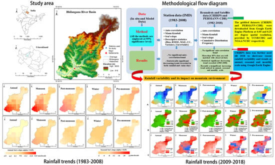
1. Introduction
- To collect, tabulate and analyse rainfall data collected from i) available surface observatories managed by IMD ii) reanalysis rainfall data from CHIRPS and iii) satellite rainfall data PERSIANN-CDR
- To map annual and seasonal time series of rainfall dynamics and juxtapose the performance of reanalysis and satellite-based data products compared to ground station data
- To evaluate annual, seasonal, and monthly distributions and trends in rainfall and rainy days and compare the results from the three sources through the application of non-parametric tests
- To briefly discuss the regional socio-economic implications of observed rainfall variability
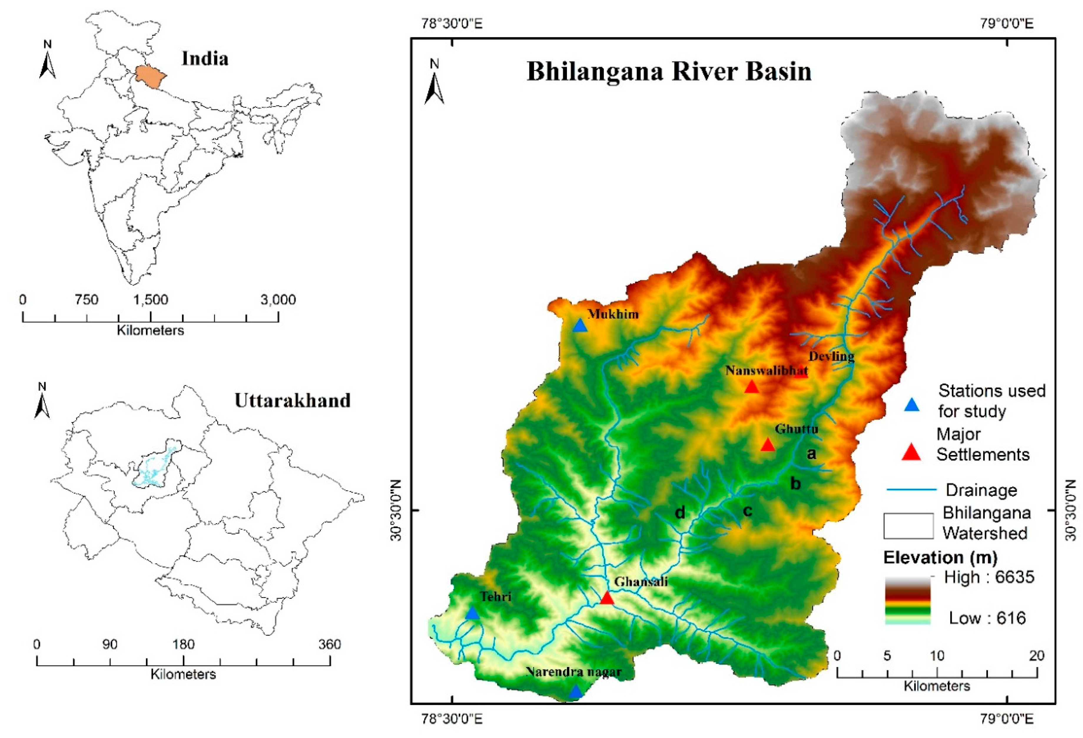
2. Environmental Characteristics of the Bhilangana River Basin
3. Materials and Methods
3.1. Observed Data
3.2. Gridded Rainfall Data
3.3. Data Handling and Statistical Applications in GEE
4. Results
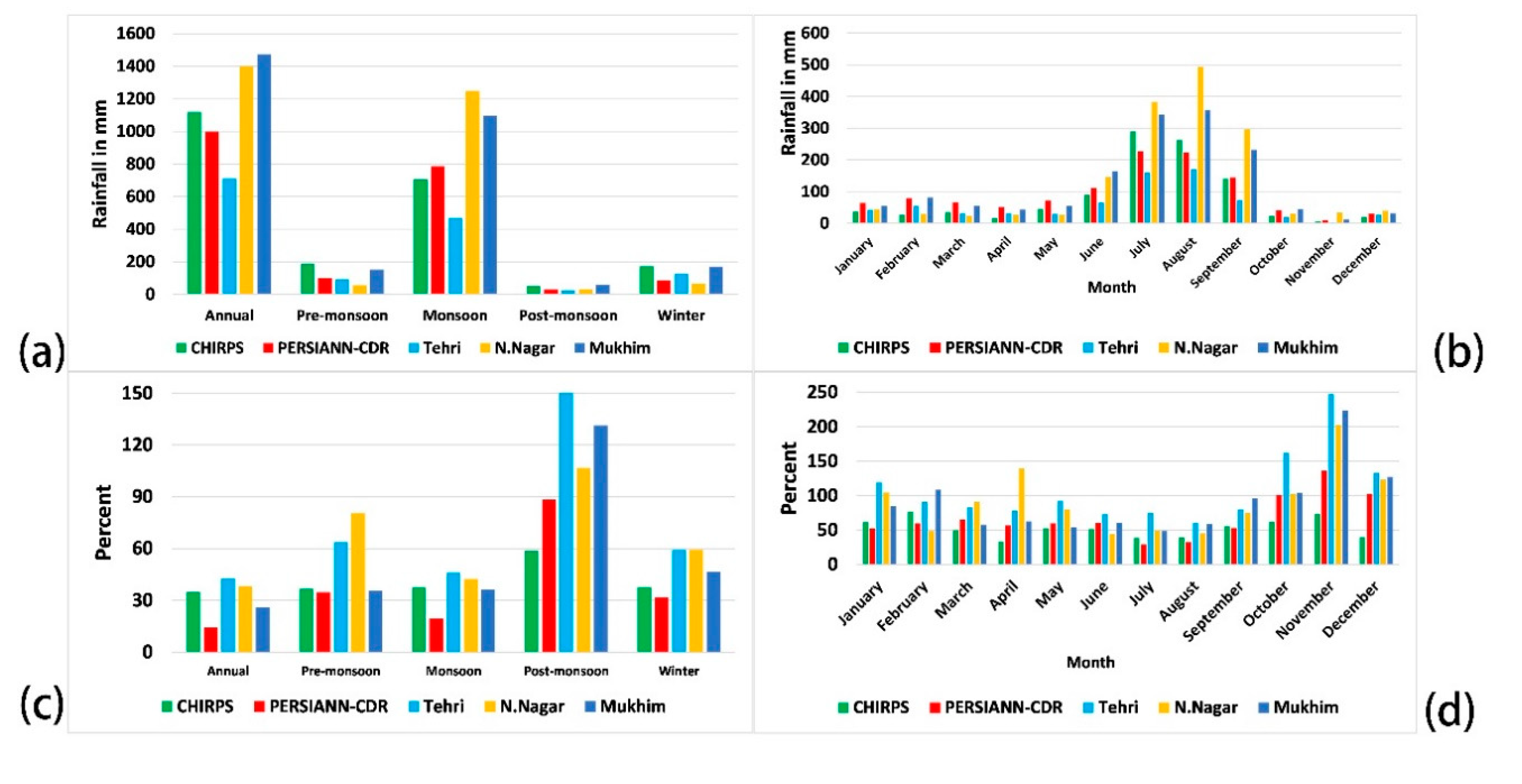
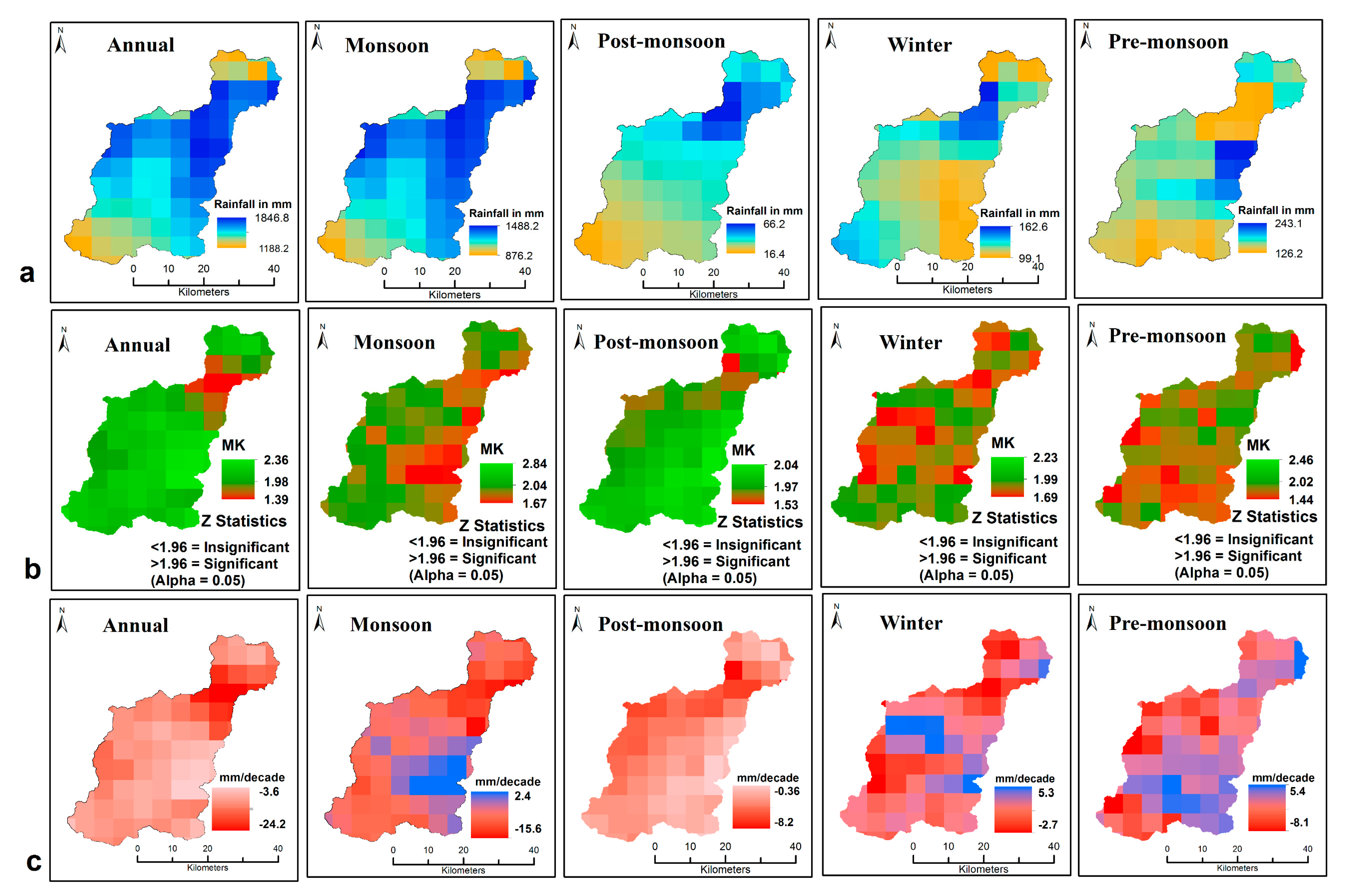
4.1. Spatio-Temporal Distribution of Rainfall and Rainy Days in the Bhilangana River Basin (1983–2008)
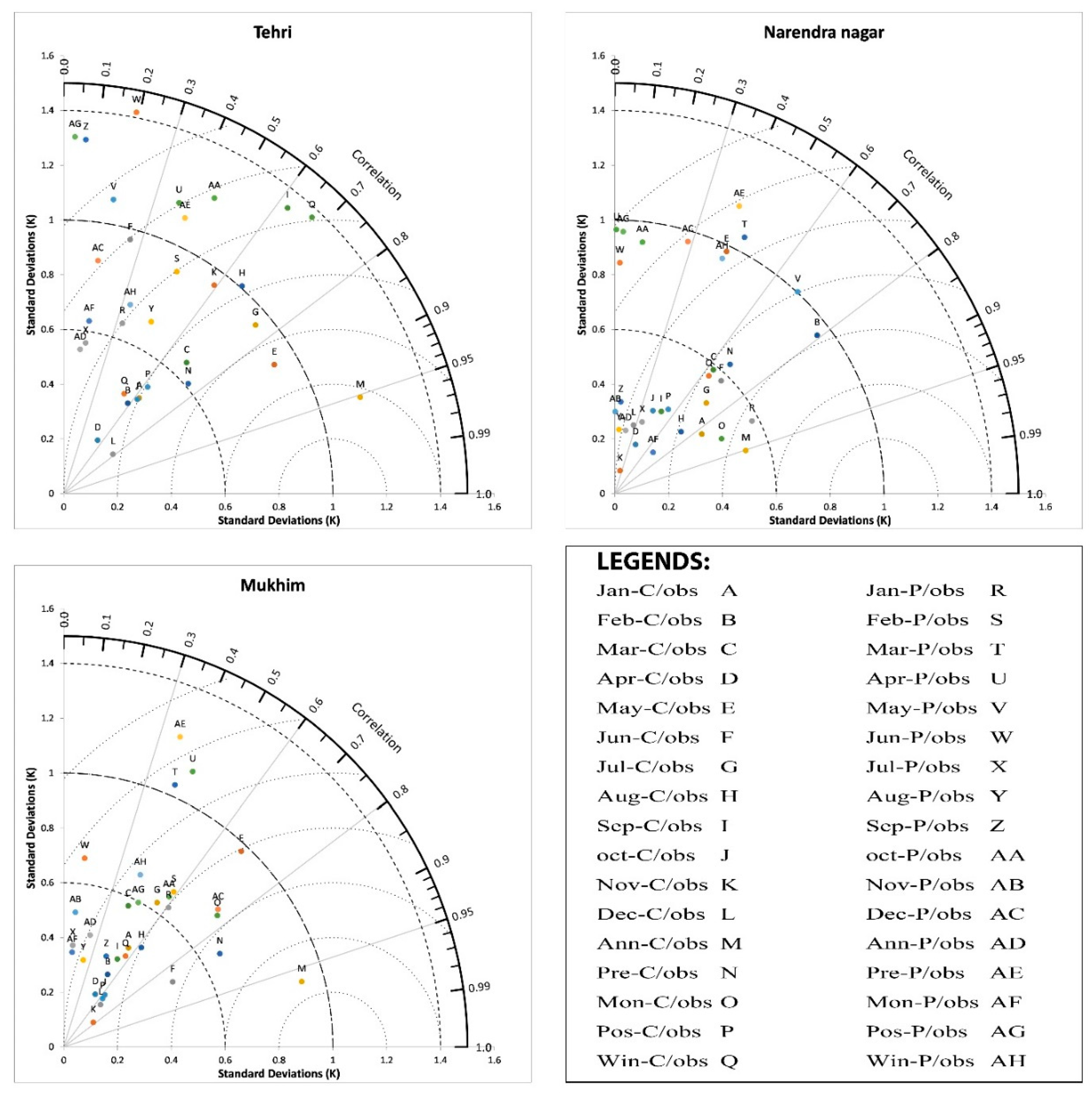
4.2. Detailed Outcomes of Descriptive Statistics
4.3. Spatio-Temporal Trends: Observational Data
4.3.1. Annual and Seasonal Trends in Observatory Rainfall Data (1983–2008)
4.3.2. Monthly Trends in Observatory Data (1983–2008)
4.3.3. Trends in Rainy Days (1983–2008)
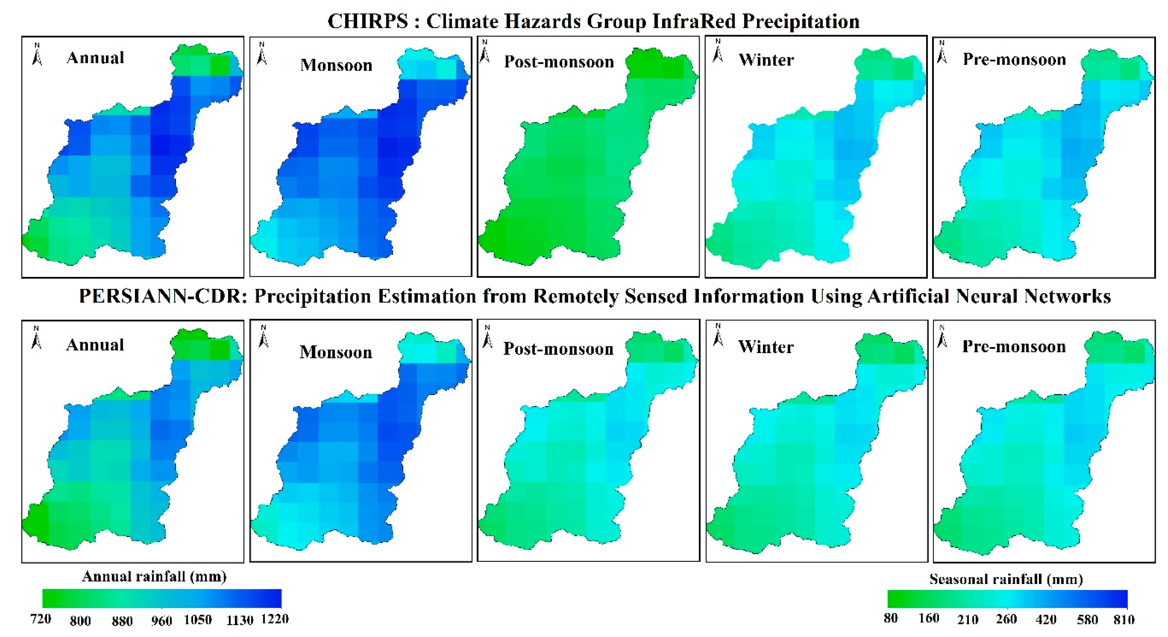
4.4. Spatio-Temporal Trends: CHIRPS and PERSIANN-CDR
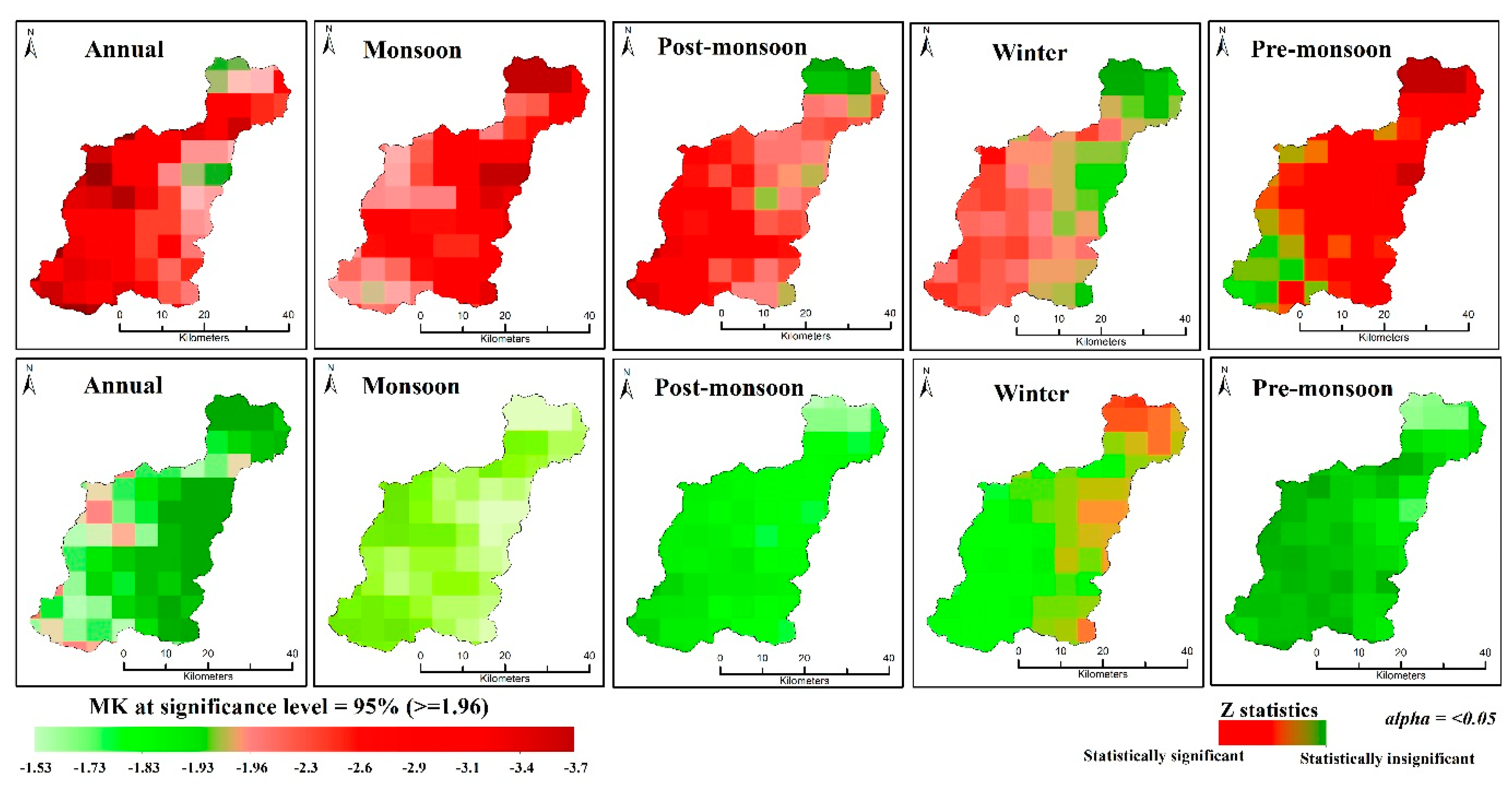
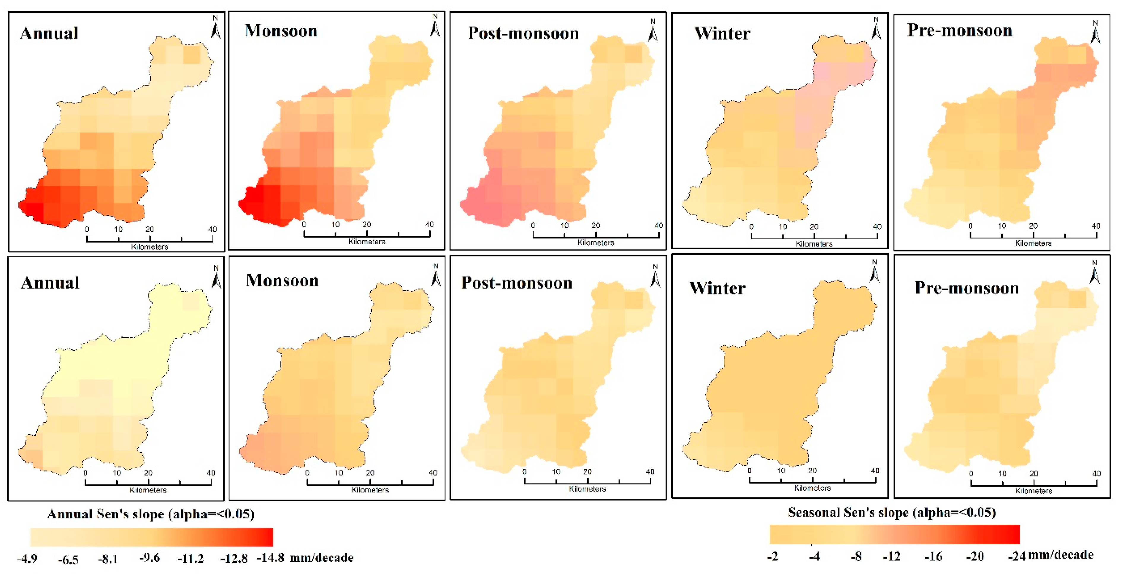
4.4.1. Annual and Seasonal Trends (1983–2008)
4.4.2. Monthly Trends: CHIRPS and PERSIANN-CDR (1983–2008)
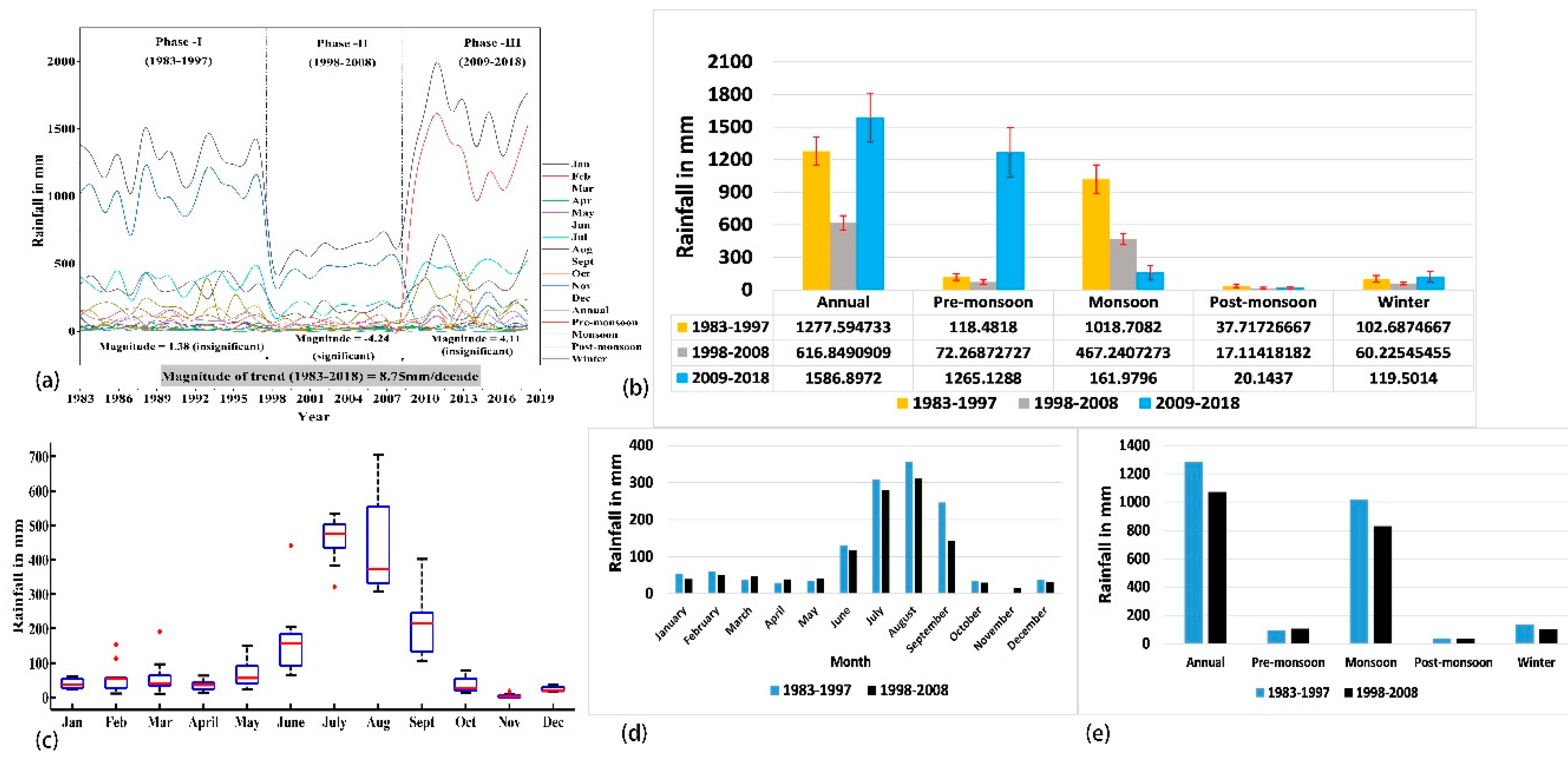
5. Inter-Annual Rainfall Variability and Trends (1983 to 2018) from Station Observed and CHIRPS Data
6. Discussion
6.1. Temporal Trends in Observed Rainfall (1983–2008)
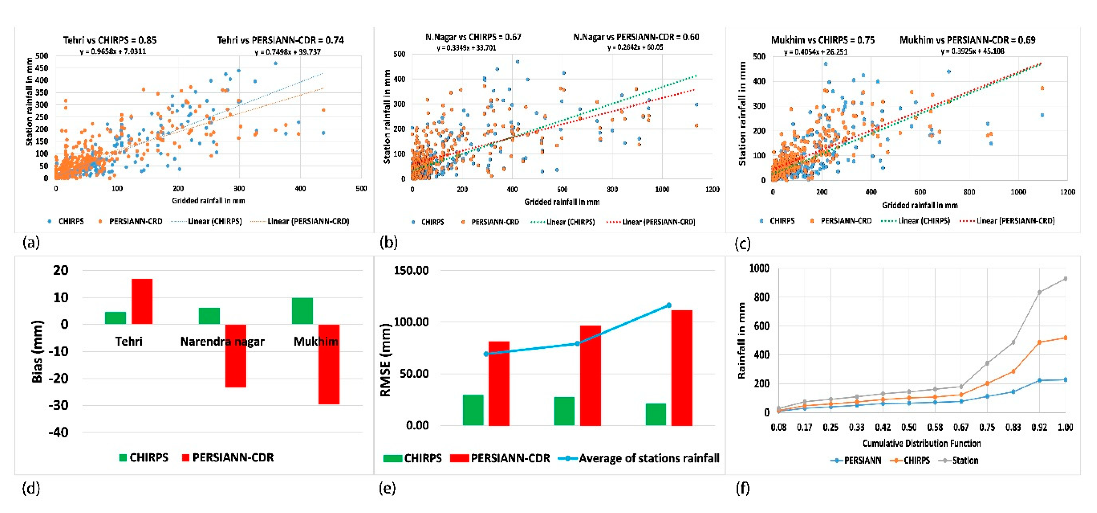
6.2. Appropriateness of Gridded Datasets in Compared to Observed Data (1983–2008)
6.3. Estimation of 1983 to 2008 Rainfall with Gridded Data
6.4. Estimation of 2009–2018 Rainfall with CHIRPS
6.5. Variability of Rainfall (1983–2018) from CHIRPS Data
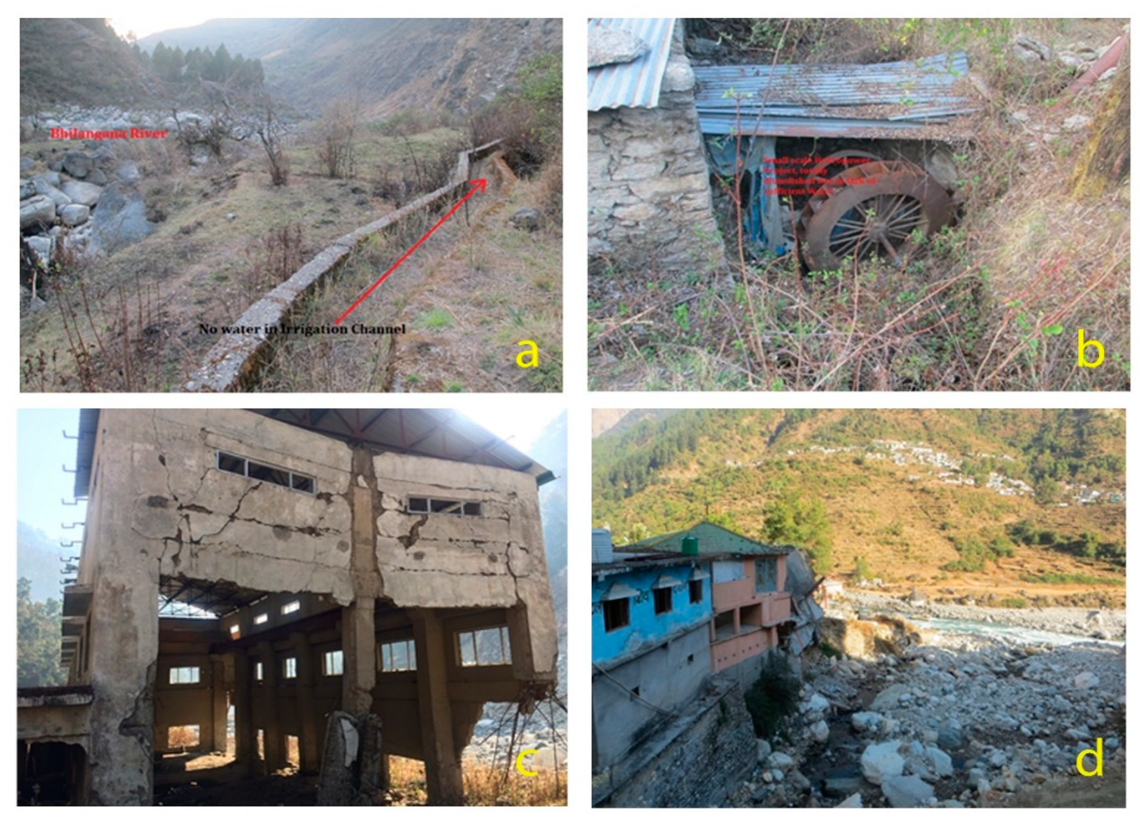
6.6. Regional Environmental Impacts of Rainfall Changes
6.6.1. Effects of Decreasing Rainfall: 1983 to 2008
6.6.2. Effects of Increasing Rainfall: 2009 to 2018
7. Conclusions
Supplementary Materials
Author Contributions
Funding
Acknowledgments
Conflicts of Interest
Abbreviations
Appendix A
Appendix A.1. Auto-Correlation
Appendix A.2. Bias
Appendix A.3. Multiplicative Bias
Appendix A.4. Relative Bias
Appendix A.5. Mean Absolute Error
Appendix A.6. Root Mean Square Error
Appendix A.7. Correlation Coefficient
Appendix A.8. Coefficient of Variation
Appendix A.9. Uncertainty
Appendix A.10. Normalised Standard Deviation
Appendix B
Appendix B.1. Mann–Kendall
Appendix B.2. Sen.’s Slope Estimation
References
- Bhatt, D.; Maskey, S.; Babel, M.S.; Uhlenbrook, S.; Prasad, K.C. Climate trends and impacts on crop production in the Koshi river basin of Nepal. Reg. Environ. Chang. 2014, 14, 1291–1301. [Google Scholar] [CrossRef] [Green Version]
- Gaddam, V.K.; Kulkarni, A.V.; Gupta, A.K. Assessment of snow-glacier melt and rainfall contribution to stream runoff in Baspa Basin, Indian Himalaya. Environ. Monit. Assess. 2018, 190, 154. [Google Scholar] [CrossRef] [PubMed]
- Chakraborty, A.; Saha, S.; Sachdeva, K.; Joshi, P.K. Vulnerability of forests in the Himalayan region to climate change impacts and anthropogenic disturbances: A systematic review. Reg. Environ. Chang. 2018, 18, 1783–1799. [Google Scholar] [CrossRef]
- Kishore, P.; Jyothi, S.; Basha, G.; Rao, S.V.B.; Rajeevan, M.; Velicogna, I.; Sutterley, T.C. Precipitation climatology over India: Validation with observations and reanalysis darasets and spatial trends. Clim. Dyn. 2016, 46, 541–556. [Google Scholar] [CrossRef] [Green Version]
- Shekhar, M.S.; Chand, H.; Kumar, S.; Srinivasan, K.; Ganju, A. Climate-change studies in the western Himalaya. Ann. Glaciol. 2010, 51, 315–322. [Google Scholar] [CrossRef] [Green Version]
- Mishra, B.; Babel, M.; Tripathi, N.K. Analysis of climate variability and snow cover in the Kaligandaki river basin, Himalaya, Nepal. Theor. Appl. Climatol. 2014, 116, 681–694. [Google Scholar] [CrossRef]
- Hoy, A.; Katel, O.; Thapa, P.; Dendup, N. Climate change and their impact on socio-economic sectors in the Bhutan Himalaya: An implementation strategy. Reg. Environ. Chang. 2016, 16, 1401–1415. [Google Scholar] [CrossRef]
- Meybeck, M.; Green, P.; Vorosmarty, C. A new topology for mountains and other relief classes. Mt. Res. Dev. 2001, 21, 34–45. [Google Scholar] [CrossRef] [Green Version]
- Hartmann, D.L.; Klein Tank, A.M.G.; Rusticucci, M.; Alexander, L.V.; Brönnimann, S.; Charabi, Y.; Dentener, F.J.; Dlugokencky, E.J.; Easterling, D.R.; Kaplan, A.; et al. Observations: Atmosphere and surface. In Climate Change 2013: The Physical Science Basis. Contribution of Working Group I to the Fifth Assessment Report of the Intergovernmental Panel on Climate Change; Stocker, T.F., Qin, D., Plattner, G.-K., Tignor, M., Allen, S.K., Boschung, J., Nauels, A., Xia, Y., Bex, V., Midgley, P.M., Eds.; Cambridge University Press: Cambridge, UK; New York, NY, USA, 2013; pp. 159–254. [Google Scholar] [CrossRef] [Green Version]
- Yadav, R.R. Tree ring evidence of a 20th century precipitation surge in the monsoon shadow zone of the western Himalaya, India. J. Geophys. Res. 2011, 116. [Google Scholar] [CrossRef]
- Bhutiyani, M.R.; Kale, S.V.; Pawar, J.N. Long-term trends in maximum, minimum and mean annual air temperatures across the Northwestern Himalaya during the twentieth century. Clim. Chang. 2007, 85, 159–177. [Google Scholar] [CrossRef]
- Dash, S.K.; Hunt, J.C.R. Variability of climate change in India. Curr. Sci. 2007, 93, 782–788. [Google Scholar]
- Basistha, A.; Arya, D.S.; Goel, N.K. Analysis of historical changes in rainfall in the Indian Himalayas. Int. J. Climatol. 2009, 29, 555–572. [Google Scholar] [CrossRef]
- Pal, I.; Al-Tabbaa, A. Long-term changes and variability of monthly extreme temperatures in India. Theor. Appl. Climatol. 2010, 100, 45–56. [Google Scholar] [CrossRef]
- Ramesh, K.V.; Goswami, P. Reduction in temporal and spatial extent of the Indian summer monsoon. Geophys. Res. Lett. 2007, 34. [Google Scholar] [CrossRef]
- Kumar, V.; Jain, S.K. Trends in rainfall amount and number of rainy days in river basins of India (1951–2004). Hydrol. Res. 2011, 42, 290. [Google Scholar] [CrossRef]
- Das, P.K.; Chakraborty, A.; Seshasai, M.V.R. Spatial analysis of temporal trend of rainfall and rainy days during the Indian Summer Monsoon season using daily gridded (0.5° × 0.5°) rainfall data for the period of 1971–2005. Meteorol. Appl. 2014, 21, 481–493. [Google Scholar] [CrossRef]
- Allen, S.; Rastner, P.; Arora, M.; Huggel, C.; Stoffel, M. Lake outburst and debris flow disaster at Kedarnath, June 2013: Hydro meteorological triggering and topographic predisposition. Landslides 2015, 13, 1479–1491. [Google Scholar] [CrossRef]
- Wang, Z.; Zhong, R.; Lai, C.; Chen, J. Evaluation of the GPM IMERG satellite-based precipitation products and the hydrological utility. Atmos. Res. 2017, 196, 151–163. [Google Scholar] [CrossRef]
- Mei, Y.W.; Anagnostou, E.N.; Nikolopoulos, E.I.; Borga, M. Error analysis of satellite precipitation products in mountainous basins. J. Hydrometeorol. 2014, 15, 1778–1793. [Google Scholar] [CrossRef]
- Guo, H.; Chen, S.; Bao, A.; Behrangi, A.; Hong, Y.; Ndayisaba, F.; Hu, J.; Stepanian, P.M. Early assessment of integrated multi-satellite retrievals for global precipitation measurement over China. Atmos. Res. 2016, 176–177, 121–133. [Google Scholar] [CrossRef]
- Sharifi, E.; Steinacker, R.; Saghafian, B. Assessment of GPM-IMERG and other precipitation products against gauge data under different topographic and climatic conditions in Iran: Preliminary results. Remote Sens. 2016, 8, 135. [Google Scholar] [CrossRef] [Green Version]
- Sidhu, N.; Pebesma, E.; Camara, G. Using Google Earth Engine to detect land cover change: Singapore as a use case. Eur. J. Remote Sens. 2018, 51, 486–500. [Google Scholar] [CrossRef]
- District Census Handbook. Village and Town Directory, Tehri Garhwal. Directorate of Census Operations, Uttarakhand; 2011; Series-06, Part XII-A; Dehradun, Uttarakhand. Available online: http://www.censusindia.gov.in (accessed on 2 December 2019).
- Auden, J.B. Director’s General Report of 1935. Rec. Geol. Surv. India Calcutta 1936, 71, 73–75. [Google Scholar]
- Agarwal, N.C.; Kumar, G. Geology of the upper Bhagirathi and Yamuna Valleys, Uttarakashi District, Kumaun Himalaya. Himal. Geol. 1973, 3, 1–23. [Google Scholar]
- Dasgupta, S.; Mazumdar, K.; Pande, P.; Sanyal, S. Seismotectonic Atlas of Indian and Its Environs; Geological Survey of India: Kolkata, India, 2000.
- Banerjee, A.; Singh, R.B.; Mal, S. Assessment of landslide hazards in mountainous terrain: A case study of Bhilangana river basin, Uttarakhand Himalaya. Hill Geog. 2018, 34, 51–61. [Google Scholar]
- Dimri, A.P.; Chevuturi, A.; Niyogi, D.; Thayyen, R.J.; Ray, K.; Tripathi, S.N.; Pandey, A.K.; Mohanty, U.C. Cloudbursts in Indian Himalaya: A review. Earth Sci. Rev. 2017, 168, 1–23. [Google Scholar] [CrossRef]
- Lopez-Carr, D.; Pricope, N.G.; Aukema, J.E.; Jankowska, M.M.; Funk, C.; Husak, G.; Michaelsen, J. A spatial analysis of population dynamics and climate change in Africa: Potential vulnerability hot spots emerge where precipitation declines and demographic presuures coincide. Popul. Environ. 2014, 35, 323–339. [Google Scholar] [CrossRef]
- Funk, C.; Peterson, P.; Landsfeld, M.; Pedreros, D.; Verdin, J.; Shukla, S.; Husak, G.; Rowland, J.; Harrison, J.; Hoell, A.; et al. The climate hazards infrared precipitation with stations—A new environmental record for monitoring extremes. Sci. Data 2015, 2, 1–21. [Google Scholar] [CrossRef] [Green Version]
- Hussain, Y.; Satge, F.; Hussain, M.B.; Carvajal, H.M.; Bonnet, M.P.; Soto, M.C.; Roig, H.L.; Akhter, G. Performance of CMORPH, TMPA and PERSIANN rainfall datasets over plain, mountains, and glacial regions of Pakistan. Theor. Appl. Climatol. 2017. [Google Scholar] [CrossRef]
- Ullah, W.; Wang, G.; Ali, G.; Hagan, D.F.T.; Bhatti, A.S.; Lou, D. Comparing multiple precipitation products against in situ observations over different climate regions of Pakistan. Remote Sens. 2018, 11, 628. [Google Scholar] [CrossRef] [Green Version]
- Prakash, S. Performance assessment of CHIRPS, MSWEP, SM2RAIN-CCI, and TMPA precipitation products across India. J. Hydrol. 2019, 57, 50–59. [Google Scholar] [CrossRef]
- Beck, H.E.; Vergopolan, N.; Pan, M.; Levizzani, V.; Albert, I.J.M.; Dijk, V.; Weedon, G.P.; Brocca, L.; Pappenberger, F.; Huffman, G.J.; et al. Global-scale evaluation of 22 precipitation datasets using gauge observations and hydrological modelling. Hydrol. Earth Syst. Sci. 2019, 21, 6201–6217. [Google Scholar] [CrossRef] [Green Version]
- Guo, H.; Chen, S.; Bao, A.; Hu, J.; Gebregiorgis, A.; Xue, X.; Zhang, X. Inter-comparison of high-resolution satellite precipitation products over Central Asia. Remote Sens. 2015, 7, 7181–7211. [Google Scholar] [CrossRef] [Green Version]
- Yang, X.; Yong, B.; Hong, Y.; Chen, S.; Zhang, X. Error analysis of multi-satellite precipitation estimates with an independent rain gauge observation network over a medium-sized humid basin. Hydrol. Sci. J. 2016, 61, 1813–1830. [Google Scholar] [CrossRef]
- Ashouri, H.; Nguyen, P.; Thorstensen, A.; Hsu, K.L.; Sorooshian, S.; Braithwaite, D. Assessing the efficacy of high-resolution satellite-based PERSIANN-CDR precipitation product in simulating streamflow. J. Hydrometeorol. 2016, 17, 2061–2076. [Google Scholar] [CrossRef]
- Mondal, A.; Lakshmi, V.; Hashemi, H. Intercomparison of trend analysis of multisatellite monthly precipitation products and gauge measurements for river basins of India. J. Hydrol. 2018, 565, 779–790. [Google Scholar] [CrossRef]
- Gorelick, N.; Hancher, M.; Dixon, M.; Llyushchenko, S.; Thau, D.; Moore, R. Google Earth Engine: Planetary-scale geospatial analysis for everyone. Remote Sens. Environ. 2017, 202, 18–27. [Google Scholar] [CrossRef]
- Vos, K.; Splinter, K.D.; Harley, M.D.; Joshua, A.S.; Turner, S.I. CoastSat: A Google Earth Engine-enabled Python toolkit to extract shorelines from publicly available satellite imagery. Environ. Model. Softw. 2019, 122, 104528. [Google Scholar] [CrossRef]
- Singh, R.B.; Mal, S. Trend and variability of monsoon and other rainfall seasons in Western Himalaya, India. Atmos. Sci. Lett. 2014, 15, 218–226. [Google Scholar] [CrossRef]
- Hamed, K.H.; Rao, A.R. A modified Mann-Kendall trend test for auto correlated data. J. Hydrol. 1998, 204, 182–196. [Google Scholar] [CrossRef]
- Kumar, M.; Denis, D.M.; Suryavanshi, S. Long-term climatic trend analysis of Giridih district, Jharkhand (India) using statistical approach. Model Earth Syst. Environ. 2016, 2, 116. [Google Scholar] [CrossRef] [Green Version]
- Zelenakova, M.; Vido, J.; Portela, M.M.; Purcz, P.; Blistan, H.H.; Hlustik, P. Precipitation trend over Slovakia in the period 1981–2013. Water 2017, 9, 922. [Google Scholar] [CrossRef] [Green Version]
- Anjum, M.N.; Ding, Y.; Shangguan, D.; Ahmad, I.; Ijaz, M.W.; Farid, H.U.; Yagoub, Y.E.; Zaman, M. Performance evalution of latest integrated multi-satellite retrievals for Global Precipitation Measurement (IMERG) over northern highlands of Pakistan. Atmos. Res. 2018, 205, 134–146. [Google Scholar] [CrossRef]
- Taylor, K.E. Summarizing multiple aspects of model performance in a single diagram. J. Geophys. Res. 2001, 106, 7183–7192. [Google Scholar] [CrossRef]
- Archer, D.R.; Fowler, H.J. Spatial and temporal variations in precipitation in the upper Indus Basin, global teleconnections and hydrological implications. Hydrol. Earth Syst. Sci. 2004, 8, 47–61. [Google Scholar] [CrossRef] [Green Version]
- Dimri, A.P.; Niyogi, D. Regional climate model application at subgrid scale on Indian winter monsoon over the western Himalaya. Int. J. Climatol. 2013, 33, 2185–2205. [Google Scholar] [CrossRef]
- Palazzi, E.; Hardeberg, J.V.; Provenzale, A. Precipitation in the Hindu-Kush Karakoram Himalaya: Bbservations and future scenarios. J. Geophys. Res. Atmos. 2013, 118, 85–100. [Google Scholar] [CrossRef]
- Paranjpye, V. (Ed.) Evaluating the Tehri Dam: An Extended Cost-Benefit Appraisal. In Indian National Trust for Art and Culture; Indian National Trust for Art and Cultural Heritage: New Delhi, India, 1988; ISBN 10: 819000610X. [Google Scholar]
- Sinha, B.K.; Pokhriyal, H.C. Rehabilitation in Tehri Dam: An evaluation. Soc. Chang. 2001, 31, 110–143. [Google Scholar] [CrossRef]
- Randhawa, M.S. (Ed.) A History of Agriculture in India. In Indian Council of Agricultural Research; Indian Council of Agricultural Research: New Delhi, India, 1986; Volume IV, Record Number 19846751450. [Google Scholar]
- Joshi, S.; Kumar, K.; Joshi, V.; Pande, B. Rainfall variability and indices of extreme rainfall-analysis and perception study for two stations over Central Himalaya, India. Nat. Hazards 2014, 72, 361–374. [Google Scholar] [CrossRef]
- Kumar, N.; Yadav, B.P.; Gahlot, S.; Singh, M. Winter frequency of western disturbances and precipitation indices over Himachal Pradesh, India: 1977–2007. Atmósfera 2015, 28, 63–70. [Google Scholar] [CrossRef]
- Gupta, R.P.; Haritashya, U.K.; Singh, P. Mapping dry/wet snow cover in the Indian Himalaya using IRS multispectral imagery. Remote Sens. Environ. 2005, 97, 458–469. [Google Scholar] [CrossRef]
- Baines, P.G. The late 1960s Global Climate Shift and its influence on the Southern Hemisphere. In Proceedings of the 8 ICSHMO, Foz do Iguaçu, Brazil, 24–28 April 2006; pp. 1477–1482. [Google Scholar]
- Lhara, C.; Kushnir, Y.; Cane, M.A.; Pene, V.D.L. Indian summer monsoon rainfall and its link with ENSO and Indian Ocean climate indices. Int. J. Climatol. 2007, 27, 179–187. [Google Scholar] [CrossRef]
- Li, H.; Haugen, J.E.; Xu, C.Y. Precipitation pattern in the Western Himalayas revealed by four datasets. Hydrol. Earth Syst. Sci. 2018, 22, 5097–5110. [Google Scholar] [CrossRef] [Green Version]
- Bollasina, M.A.; Ming, Y.; Ramaswamy, V. Anthropogenic Aerosols and the Weakening of the South Asian Summer Monsoon. Science 2011, 334, 502–505. [Google Scholar] [CrossRef] [PubMed] [Green Version]
- Chiao, S.; Lin, Y.L.; Kaplan, M.L. Numerical study of orographic forcing of heavy precipitation during MAP IOP-2B. Mon. Weather Rev. 2004, 132, 2184–2203. [Google Scholar] [CrossRef]
- Barros, A.P.; Kim, G.; Williams, E.; Nesbitt, S.W. Probing orographic controls in the Himalayas during the monsoon using satellite imagery. Nat. Hazards Earth Syst. Sci. 2004, 4, 29–51. [Google Scholar] [CrossRef] [Green Version]
- Chen, J.; Li, C.; He, G. A diagnostic analysis of the impact of complex terrain in the Eastern Tibetan Plateau, China, on a severe storm, Arctic. Arct. Antarct. Alp. Res. 2007, 39, 699–707. [Google Scholar] [CrossRef] [Green Version]
- Medina, S.; Houze, R.A., Jr.; Kumar, A.; Niyogi, D. Summer monsoon convection in the Himalayan region: Terrain and land cover effects. Q. J. R. Meteorol. Soc. 2010, 136, 593–616. [Google Scholar] [CrossRef] [Green Version]
- Bhardwaj, A.; Ziegler, A.D.; Wasson, R.J.; Chow, W.T.L. Accuracy of rainfall estimates at high altitude in the Garhwal Himalaya (India): A comparison of secondary precipitation products and station rainfall measurements. Atmos. Res. 2017, 188, 30–38. [Google Scholar] [CrossRef]
- Bhuiyan, M.A.E.; Nikolopoulos, E.I.; Anagnostou, E.N.; Pere, Q.S.; Ortiz, A.B. A nonparametric statistical technique for combining global precipitation datasets: Development and hydrological evaluation over the Iberian Peninsula. Hydrol. Earth Syst. Sci. 2018, 22, 1371–1389. [Google Scholar] [CrossRef] [Green Version]
- Ba, K.M.; Balcazar, L.; Diaz, V.; Qrtiz, F.; Miguel, A.G.; Carlos, D.D. Hydrological evaluation of PERSIANN-CDR rainfall over Upper Senegal River and Bani River basins. Remote Sens. 2018, 10, 1884. [Google Scholar] [CrossRef] [Green Version]
- Liu, J.; Xu, Z.; Junrui, B.; Peng, D.; Ren, M. Assessment and correction of the PERSIANN-CDR product in the Yarlung Zangbo River basin, China. Remote Sens. 2018, 10, 2031. [Google Scholar] [CrossRef] [Green Version]
- Sun, S.; Zhou, S.; Shen, H.; Chai, R.; Chen, H.; Liu, Y.; Shi, W.; Wang, J.; Wang, G.; Zhou, Y. Dissecting performance of PERSIANN-CDR precipitation product over Huai River basin, China. Remote Sens. 2019, 11, 1805. [Google Scholar] [CrossRef] [Green Version]
- Romatschke, U. Regional, seasonal, and diurnal variations of extreme convection in the south Asian region. J. Clim. 2010, 23, 419–439. [Google Scholar] [CrossRef] [Green Version]
- Bharti, V.; Singh, C. Evaluation of error in TRMM 3B42V7 precipitation estimates over the Himalaya region. J. Geophy. Res. Atmos. 2015, 120, 458–473. [Google Scholar] [CrossRef]
- IPCC. 2013: Climate Change 2013: The Physical Science Basis. In Contribution of Working Group I to the Fifth Assessment Report of the Intergovernmental Panel on Climate Change; Stocker, T.F., Qin, D., Plattner, G.-K., Tignor, M., Allen, S.K., Boschung, J., Nauels, A., Xia, Y., Bex, V., Midgley, P.M., Eds.; Cambridge University Press: Cambridge, UK; New York, NY, USA, 2013; p. 1535. [Google Scholar] [CrossRef] [Green Version]
- Lutz, A.F.; Immerzeel, W.W.; Shrestha, A.B.; Bierkens, M.F.P. Consistent increase in High Asia’s runoff due to increasing glacier melt and precipitation. Nat. Clim. Chang. 2014, 4, 587–592. [Google Scholar] [CrossRef] [Green Version]
- Apollo, M. The population of Himalayan regions—By the numbers: Past, present and future. In Contemporary Studies in Environment and Tourism; Efe, R., Ozturk, M., Eds.; Cambridge Scholar Publishing: Cambridge, UK, 2017; pp. 145–159. ISBN 978-1-4438-7283-6. [Google Scholar]
- Sharma, C.; Ojha, C.S.P.; Shukla, A.K.; Pham, Q.B.; Linh, N.T.T.; Fai, C.M.; Ho, H.L.; Dung, T.D. Modified approach to reduce GCM bias in downscaled Precipitation: A study in Ganga River basin. Water 2019, 11, 2097. [Google Scholar] [CrossRef] [Green Version]
- Maan, H.B. Non-parametric tests against trend. Econometrica 1945, 33, 245–259. [Google Scholar] [CrossRef]
- Kendall, M.G. Rank Correlation Method, 4th ed.; Charles Griffin: London, UK, 1975. [Google Scholar]
- Jhajharia, D.; Dinpashoh, Y.; Kahya, E.; Chowdhury, R.R.; Singh, P.V. Trends in temperature over Godavari River basin in Southern Peninsular India. Int. J. Climatol. 2014, 34, 1369–1384. [Google Scholar] [CrossRef]
- Jhajharia, D.; Singh, P.V. Trends in temperature, diurnal temperature range and sunshine duration in Northeast India. Int. J. Climatol. 2011, 31, 1353–1367. [Google Scholar] [CrossRef]
- Drapela, K.; Drapelova, I. Application of Mann-Kendall test and the Sen’s slope estimates for trend detection in deposition data from Bily Kriz (Beskydy Mts, the Czech Republic) 1997–2010. Beskydy 2011, 4, 133–146. [Google Scholar]
- Sen, P.K. Estimates of the regression coefficient based on Kendall’s tau. J. Am. Stat. Assoc. 1968, 63, 1379–1389. [Google Scholar] [CrossRef]


| Station Observed Data (Collected from IMD) | |||||
|---|---|---|---|---|---|
| Station | Location | Period | Elevation (m) | Available Observations (%) | |
| Lat. | Long. | ||||
| Mukhem | 30.34 | 78.28 | 1983–2008 | 1981 | 95.8 |
| Tehri | 30.22 | 78.26 | 1983–2008 | 676 | 91.3 |
| Narendra Nagar | 30.09 | 78.17 | 1983–2008 | 1037 | 81.3 |
| Gridded Data (Downloaded through Google Earth Engine Platform) | |||||
| Data product | Year | Source | Grid Spacing | ||
| CHIRPS | 1983–2018 | UCSB/CHG | 0.05 arc degree | ||
| PERSIANN-CDR | 1983–2008 | NOAA/NCDC | 0.25 arc degree | ||
| Data | JAN | FEB | MAR | APR | MAY | JUN | JUL | AUG | SEPT | OCT | NOV | DEC |
| Station | 63.7 | 78.3 | 66.8 | 50.6 | 71.3 | 112.3 | 227.9 | 223.8 | 144.5 | 40.0 | 10.3 | 30.3 |
| CHIRPS | 36.8 | 27.1 | 35.4 | 17.4 | 46.1 | 90.0 | 290.6 | 263.8 | 141.0 | 23.6 | 5.4 | 20.8 |
| PERSIANN-CDR | 55.7 | 54.9 | 40.4 | 31.7 | 36.1 | 140.5 | 347.1 | 410.5 | 201.5 | 42.4 | 13.4 | 28.1 |
| Data | Annual | Pre-monsoon | Monsoon | Post-monsoon | Winter | |||||||
| Station | 1313.4 | 154.3 | 1014.8 | 48.3 | 96.0 | |||||||
| CHIRPS | 1119.7 | 188.7 | 708.6 | 50.3 | 172.3 | |||||||
| PERSIANN-CDR | 998.0 | 98.9 | 785.4 | 29.1 | 87.7 | |||||||
| Statistical Indices with Units | CHIRPS | PERSIANN-CDR | ||||
|---|---|---|---|---|---|---|
| Tehri | N.Nagar | Mukhim | Tehri | N.Nagar | Mukhim | |
| RMSE (mm) | 29.60 | 24.66 | 21.58 | 81.24 | 96.20 | 111.30 |
| MAE (mm) | 30.20 | 26.31 | 66.54 | 49.76 | 83.09 | 66.54 |
| Bias (mm) | 4.59 | 6.26 | 9.88 | 16.88 | −23.4 | −29.5 |
| MBias (mm) | 0.93 | 0.99 | 1.62 | 0.77 | 2.11 | 1.61 |
| RBias (%) | 0.06 | 0.08 | 0.41 | 0.29 | 0.35 | 0.39 |
| CC | 0.85 | 0.67 | 0.69 | 0.74 | 0.60 | 0.75 |
| Station | Sen.’s Slope (mm/decade) | |||||
|---|---|---|---|---|---|---|
| Annual | Monsoon | Post-Monsoon | Winter | Pre-Monsoon | ||
| Mukhim | Distribution | 1473.7 | 1095.8 | 56.7 | 169.9 | 151.2 |
| Trend | −2.04 | −3.79 | −0.88 | −0.01 | −0.68 | |
| Tehri | Distribution | 710.8 | 469.9 | 22.2 | 125.6 | 92.9 |
| Trend | −12.26 | −7.46 | 0.00 | −0.71 | −0.31 | |
| Narendra Nagar | Distribution | 1400.4 | 1249.9 | 29.5 | 65.5 | 55.5 |
| Trend | −32.82 | −22.37 | −0.82 | −2.56 | −0.95 | |
| Station | JAN | FEB | MAR | APR | MAY | JUN | JUL | AUG | SEPT | OCT | NOV | DEC | |
|---|---|---|---|---|---|---|---|---|---|---|---|---|---|
| Mukhim | Distribution | 56.2 | 81.5 | 53.8 | 42.8 | 54.6 | 163.4 | 342.9 | 357.9 | 231.7 | 45.0 | 11.7 | 32.3 |
| Trend | −0.34 | 0.71 | 0.20 | 0.42 | 0.42 | −0.31 | −0.70 | 0.62 | 0.10 | −0.60 | 0.00 | 0.00 | |
| Tehri | Distribution | 42.5 | 56.0 | 32.0 | 32.0 | 29.0 | 66.0 | 159.8 | 170.4 | 73.7 | 20.5 | 1.7 | 27.1 |
| Trend | −0.13 | −0.00 | −0.00 | −0.00 | −0.11 | 0.10 | −0.80 | −0.10 | −0.11 | −0.10 | 0.00 | 0.00 | |
| Narendra Nagar | Distribution | 43.7 | 29.2 | 23.3 | 26.5 | 28.0 | 145.7 | 382.7 | 493.7 | 296.2 | 30.5 | 33.1 | 39.6 |
| Trend | −0.62 | −0.42 | −0.70 | 0.00 | −0.30 | −0.91 | −8.43 | −12.40 | −2.92 | −0.51 | 0.00 | 0.00 |
| Station | Annual | Monsoon | Post-Monsoon | Winter | Pre-Monsoon |
|---|---|---|---|---|---|
| Mukhim | −6 | −8 | −2 | −1 | 0.00 |
| Tehri | −7 | −3 | 0.00 | 0.00 | 0.00 |
| Narendra Nagar | −9 | −11 | 0.00 | 0 | 0.00 |
| Data | Annual | Monsoon | Post-Monsoon | Winter | Pre-Monsoon |
|---|---|---|---|---|---|
| CHIRPS | −14.82 | −24.14 | −9.60 | −12.60 | −3.12 |
| PERSIANN-CRD | −6.91 | −5.12 | −0.71 | −2.91 | −1.32 |
| DATA | JAN | FEB | MAR | APR | MAY | JUN | JUL | AUG | SEPT | OCT | NOV | DEC |
|---|---|---|---|---|---|---|---|---|---|---|---|---|
| CHIRPS | −1.08 | −0.51 | −1.13 | 0.12 | −1.60 | −3.10 | −9.42 | −9.44 | −5.71 | −0.81 | −0.30 | −0.42 |
| PERSIANN-CDR | −1.11 | −0.12 | −0.50 | −0.60 | 1.21 | 1.42 | −2.31 | −3.50 | −0.60 | 1.12 | −0.11 | −1.41 |
| Distribution | JAN | FEB | MAR | APR | MAY | JUN | JUL | AUG | SEPT | OCT | NOV | DEC |
|---|---|---|---|---|---|---|---|---|---|---|---|---|
| 1983–2008 (CHIRPS) | 36.82 | 27.11 | 35.44 | 17.44 | 46.11 | 89.90 | 290.60 | 263.83 | 141.11 | 23.61 | 5.60 | 20.84 |
| 1983–2008 (Station) | 47.4 | 55.6 | 36.4 | 33.8 | 37.2 | 125.0 | 295.1 | 340.6 | 200.6 | 32.0 | 15.5 | 33.0 |
| 2009–2018 (CHIRPS) | 40.6 | 55.5 | 58.91 | 35.62 | 67.52 | 161.62 | 460.92 | 434.82 | 207.92 | 36.33 | 3.91 | 2.42 |
| Relative Uncertainty | 11.4 | 15.9 | 3.9 | 3.6 | 3.2 | 6.5 | 0.3 | 0.1 | 3.0 | 15.9 | 18.2 | 16.3 |
| Sen’s slope using CHIRPS (2009–2018) | 0.79 | −2.1 | 2.91 | 1.61 | 3.69 | 7.54 | 6.09 | −2.02 | −8.21 | −1.88 | −0.06 | −1.18 |
© 2020 by the authors. Licensee MDPI, Basel, Switzerland. This article is an open access article distributed under the terms and conditions of the Creative Commons Attribution (CC BY) license (http://creativecommons.org/licenses/by/4.0/).
Share and Cite
Banerjee, A.; Chen, R.; E. Meadows, M.; Singh, R.B.; Mal, S.; Sengupta, D. An Analysis of Long-Term Rainfall Trends and Variability in the Uttarakhand Himalaya Using Google Earth Engine. Remote Sens. 2020, 12, 709. https://0-doi-org.brum.beds.ac.uk/10.3390/rs12040709
Banerjee A, Chen R, E. Meadows M, Singh RB, Mal S, Sengupta D. An Analysis of Long-Term Rainfall Trends and Variability in the Uttarakhand Himalaya Using Google Earth Engine. Remote Sensing. 2020; 12(4):709. https://0-doi-org.brum.beds.ac.uk/10.3390/rs12040709
Chicago/Turabian StyleBanerjee, Abhishek, Ruishan Chen, Michael E. Meadows, R.B. Singh, Suraj Mal, and Dhritiraj Sengupta. 2020. "An Analysis of Long-Term Rainfall Trends and Variability in the Uttarakhand Himalaya Using Google Earth Engine" Remote Sensing 12, no. 4: 709. https://0-doi-org.brum.beds.ac.uk/10.3390/rs12040709