Understanding Intra-Annual Dynamics of Ecosystem Services Using Satellite Image Time Series


Faculty of Geo-information Science and Earth Observation, (ITC), University of Twente, P.O. Box 217, 7500 AE Enschede, The Netherlands
*
Author to whom correspondence should be addressed.
Remote Sens. 2020, 12(4), 710; https://0-doi-org.brum.beds.ac.uk/10.3390/rs12040710
Submission received: 25 January 2020
/
Revised: 14 February 2020
/
Accepted: 17 February 2020
/
Published: 21 February 2020
(This article belongs to the Special Issue Mapping Ecosystem Services Flows and Dynamics Using Remote Sensing)
Abstract
:Landscape processes fluctuate over time, influencing the intra-annual dynamics of ecosystem services. However, current ecosystem service assessments generally do not account for such changes. This study argues that information on the dynamics of ecosystem services is essential for understanding and monitoring the impact of land management. We studied two regulating ecosystem services (i. erosion prevention, ii. regulation of water flows) and two provisioning services (iii. provision of forage, iv. biomass for essential oil production) in thicket vegetation and agricultural fields in the Baviaanskloof, South Africa. Using models based on Sentinel-2 data, calibrated with field measurements, we estimated the monthly supply of ecosystem services and assessed their intra-annual variability within vegetation cover types. We illustrated how the dynamic supply of ecosystem services related to temporal variations in their demand. We also found large spatial variability of the ecosystem service supply within a single vegetation cover type. In contrast to thicket vegetation, agricultural land showed larger temporal and spatial variability in the ecosystem service supply due to the effect of more intensive management. Knowledge of intra-annual dynamics is essential to jointly assess the temporal variation of supply and demand throughout the year to evaluate if the provision of ecosystem services occurs when most needed.

1. Introduction
Agricultural land use, including arable lands, permanent meadows, and pastures, represents 37% of the ice-free global land surface [1]. These landscapes provide and simultaneously depend on ecosystem services that are essential for human wellbeing [2,3]. However, land degradation affects 40% of the agricultural land on earth, reducing the provision of ecosystem services and resulting in adverse environmental, social, and economic consequences [4,5,6]. Given the increased pressure on ecosystem services, numerous projects and research groups are working to improve the understanding and management of these services [7]. The ecosystem services concept is included in local, national, and international policies and their supply is a prerequisite to meet the Sustainable Development Goals [8]. During the last decades, and especially since the publication of the Millennium Ecosystem Assessment [9], there has been a noticeable increase in the use of the ecosystem service approach as an explicit decision and policy-making tool [10,11,12,13].
The ecosystem service supply is not static but depends on the dynamic structures and functions of ecosystems [14]. Weather fluctuations throughout the year affect the biophysical conditions that determine the intra-annual supply of ecosystem services, especially those that depend directly on green biomass production, such as the provision of forage [15] and crop productivity [16,17]. Soil conditions are also subject to seasonal fluctuations as a consequence of hydrological processes, such as water redistribution and runoff, that contribute to soil erosion [18,19,20]. However, studies of ecosystem services tend to produce fixed estimates, with little consideration of how ecosystem services fluctuate over time [21,22,23,24].
Monitoring the spatial and temporal aspects of ecosystem services is identified as being essential for current science-policy bodies, like the Intergovernmental Science-Policy Platform on Biodiversity and Ecosystem Services (IPBES), to enable evidence-based decisions regarding land restoration and nature conservation [25,26]. However, the temporal variability of ecosystem services is a critically under-studied aspect of ecosystem service assessments [27]. The static approach cannot provide insight into whether and how the provision of ecosystem services change over time and if their supply occurs when they are most needed [28]. In addition, the temporal information of ecosystem services is relevant to evaluate the capacity of ecosystems to recover from unfavorable conditions, adapt to ongoing change, and maintain their supply over time, i.e., to estimate resilience [29,30,31]. Considering the temporal variability of the ecosystem service supply is also important because often its demand, driving forces, and relations to human behavior change [32,33,34].
Remote sensing (RS) plays a key role in studying complex environmental interactions between natural and social systems [35]. Satellite sensors are well-suited for temporal monitoring as they provide consistent and repeatable measurements over extensive regions [36]. The ecosystem service supply can be quantified by linking remotely sensed data, such as vegetation indices, with field observations using, for example, semi-empirical regression models [37] or mechanistic approaches [38]. Vegetation indices from satellite sensor images are an important data source for quantifying ecosystem services [35], and have been used to assess, for example, the provision of forage [15,39,40], erosion prevention [41], and primary crop production [42,43,44]. However, the majority of ecosystem service delivery models are based on thematic land-use/land-cover maps, generating spatial generalization errors and the exclusion of functional trait variation within vegetation types [24,45]. Directly linking in situ observations of ecosystem services with remotely sensed data may better capture their spatio-temporal variation as compared to the often-used practice of linking the service supply directly to one land cover class [22,40].
Optical satellite sensors have trade-offs between spatial, temporal, and spectral resolutions [46]. However, over the last decade, considerable progress has been made in the development of new platforms, sensors, and techniques that can substantially improve the assessment of temporal variability at much more detailed spatial scales [47,48]. New opportunities for long-term and high-frequency monitoring applications are now arising due to the availability of a new generation of multispectral medium spatial resolution sensors [49], such as Sentinel-2 from the European Copernicus program. The two identical Sentinel-2 satellites provide an unprecedented amount of information at a relatively fine spatial resolution (10 to 60 m) and a five-day revisit time, offering enhanced opportunities for assessing the spatial distribution and temporal dynamics of biophysical variables [50,51,52]. Although the free and frequent data provided by Sentinel-2 show clear potential for spatio-temporal assessments of ecosystem services, remote sensing information is still typically lacking in ecosystem service studies [24,53].
By considering and estimating temporal changes in ecosystem service provision in relation to their demand, our study contributes to a better understanding of spatial and intra-annual distribution of ecosystem services to support site-specific management and efficient monitoring of large rural areas. The specific aims of this research study were to (1) describe intra-annual variations in ecosystem service supply using Sentinel-2 images, and (2) illustrate the relationships between intra-annual variations in the supply and the demand for ecosystem services, using a study area in South Africa.
2. Materials and Methods
2.1. Study Area
Our case study was situated in the central and eastern area of the Baviaanskloof Hartland Bawarea Conservancy (approximately 31,500 ha), Eastern Cape in South Africa (Figure 1). The study area is located between the Baviaanskloof and the Kouga mountains and is surrounded by the Baviaanskloof Nature Reserve and the Beakosneck Private Nature Reserve. This region consists of a mixture of large private farms (from 500 to 7600 hectares in size) and rural communal land. The primary income of farmers comes from extensive livestock farming, crops, and tourism [54]. Local communities live and share common land in the Baviaanskloof valley [55]. The mean annual rainfall amount in the area is 327 mm in the last 30 years, with an erratic distribution across and within years [56] (Figures S1 and S2). Water is scarce and recurring droughts are often followed by flood events [57]. The average annual temperature in the area is 17 °C. Temperatures of up to 40 °C are frequently reported around December to February, whereas between June and August temperatures may occasionally fall below 0 °C [58].
In the study area, we focused on the subtropical arid thicket areas, where spekboom (Portulacaria afra) is a dominant and heavily grazed species [59]. We also included pastures and fields planted with rosemary for essential oil production. In this area, thicket has been heavily degraded due to unsustainable pastoralism [60,61]. Since spekboom is a succulent species that propagates vegetatively [62], spontaneous recovery does not occur in heavily degraded sites [63,64]. Land degradation has resulted in severe and widespread soil erosion [58]. The reduction of the natural vegetation, which is the common source of food for the extensively farmed goat and sheep in the area, has also contributed to a dramatic decline in agricultural returns in recent years. Also, the degradation of succulent thicket affects water infiltration by decreasing the proportion of the soil surface covered with plant litter [63]. For more than a decade, the planting of spekboom cuttings has been implemented as a practical method of restoration in the area [61,65,66,67]. Several farmers in the study area are transitioning from extensive goat and sheep farming to more sustainable farming activities, such as essential oil production and tourism. This transition is made in partnership with three local and international non-governmental organizations that are active in the study area, i.e., (1) Living Lands (https://livinglands.co.za), (2) Grounded (https://www.grounded.co.za), and (3) Commonland (https://www.commonland.com), which are local and international non-governmental organizations. These organizations support large-scale and long-term restoration and sustainable land use initiatives. Essential oil production is considered a more sustainable farming practice in the area as it requires limited water and fertilizer inputs and needs less land to be profitable, compared to goat farming.
2.2. Workflow
We selected four ecosystem services (Table 1) based on recent management objectives that aim to overcome local environmental challenges related to land degradation. We considered two regulating services, i.e., erosion prevention and regulation of water flows, and two provisioning services, i.e., the provision of forage and biomass for essential oil production. Thicket vegetation was evaluated for the supply of erosion prevention, regulation of water flows, and provision of forage. Even with the current transition from extensive livestock farming towards essential oil farming, forage is still a valuable ecosystem service in the area, not only for small livestock but also for wildlife species. We excluded irrigated agricultural land for the estimation of the regulation of water flows in order to prevent disruptions in the calculated infiltration levels due to heterogeneous initial soil moisture.
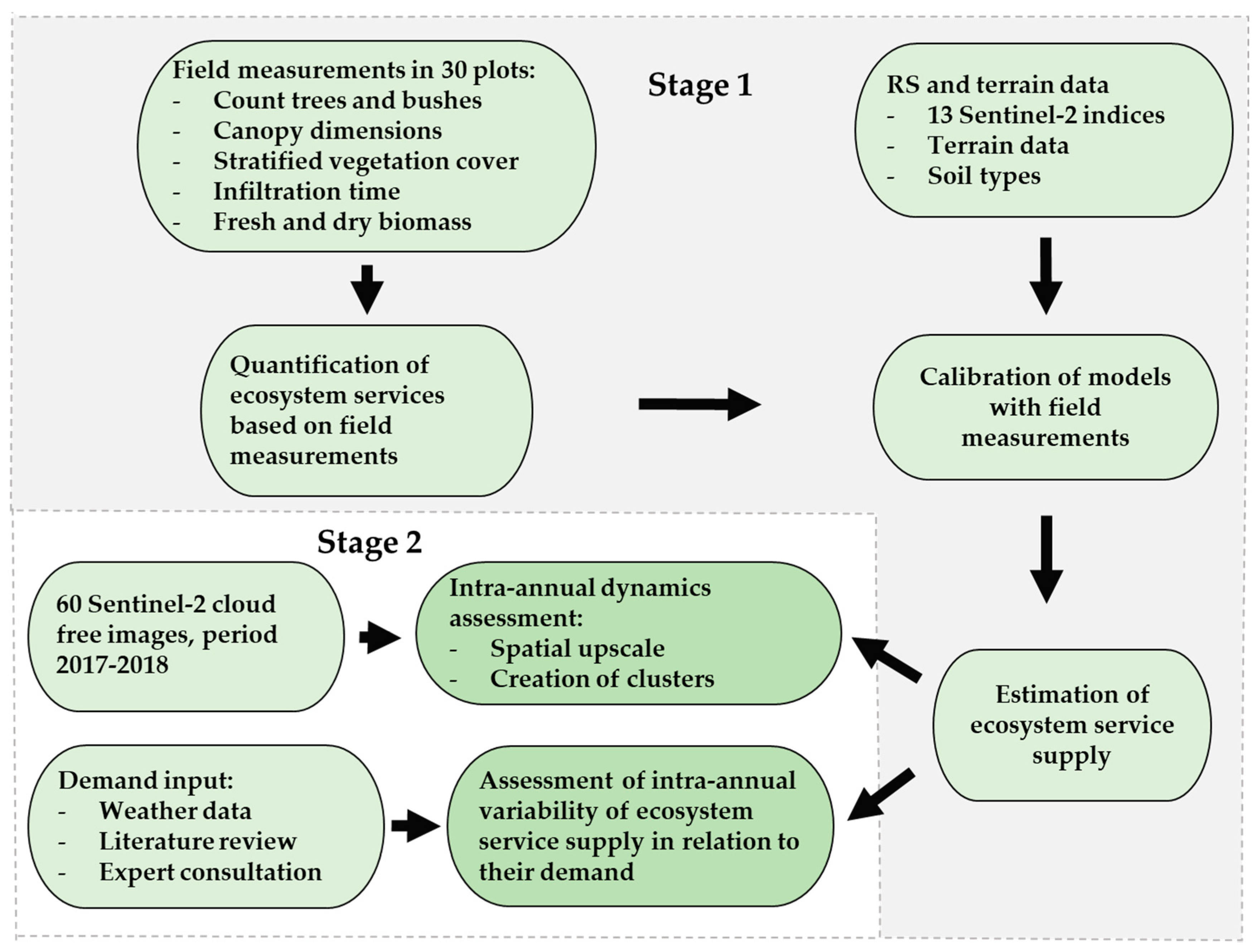
The general workflow of this study is presented in Figure 2. The first stage consisted of (1) collecting field, RS, and soil and terrain data; (2) calibrating Sentinel-2 models; and (3) estimating the supply of ecosystem services. This first stage is summarized in Section 2.2. and described in a previous study aiming to compare restoration interventions [68]. The second stage involved a temporal variability assessment in relation to the demand side of the studied ecosystem services.
2.3. RS to Capture Ecosystem Service Supply over Space and Time
To estimate ecosystem services indicators and build the models, we measured canopy dimensions, canopy cover, and infiltration in 30 plots distributed within the study area (Table 2). Plots were sampled in pairs, ensuring a similar slope angle, orientation, and geographical vicinity to avoid wide variations in soil and weather conditions. To validate the models, we used five-fold cross-validation, which we repeated 100 times [69]. Given the low number of plots, separating the 30 samples into training and validation samples would not be a valid approach, thus justifying the use of k-fold cross-validation. We combined the field-measured fractional vegetation cover of various forms of vegetation to calculate the stratified vegetation cover and quantify erosion prevention [41]. We measured the soil infiltration rates under different vegetation cover to assess the potential regulation of water flows, as infiltration levels in successfully revegetated landscapes are expected to increase over time due to higher soil macropores [70]. We used a previously developed allometric equation to estimate the biomass of rosemary based on the measured canopy dimensions [68], and to estimate the green biomass based on the measured vegetation cover for grasses and shrubs [71]. We used the calculated fresh plant biomass as an indicator for the production of essential oil derivatives and the green biomass to quantify the production of forage. Using the field-based ecosystem service estimations, we calibrated and tested the ability of the models to estimate ecosystem services based on 13 indices derived from Sentinel-2 level 2A images and a digital elevation model (see Section 2.3).
The second stage consisted of calculating the supply of ecosystem services for the whole study area using the models in Table 2 and estimating the variation of their supply for the years 2017 and 2018. To quantify how much the ecosystem service supply varies over time at the pixel level, we calculated per pixel the temporal standard deviation of each ecosystem service, separately for the years 2017 and 2018. We used a vegetation map as input to assess the supply of ecosystem services for all thicket vegetation in the area [72]. In some cases, built-up, agricultural areas, or vegetation along the river were misclassified as thicket on the vegetation map. To improve the vegetation map, the thicket cover class was manually corrected using vector files of rivers, roads, and agricultural lands provided by Living Lands (Table 3). We used Google Earth Pro to correct misclassified thicket vegetation in built-up areas.
We applied the ecosystem service models under the assumption that the RS models calibrated with the field data of 30 sampled plots can be spatially and temporally extrapolated to areas with the same vegetation type, similar land management, landscape, and weather characteristics. Using the collected data of rosemary fields from 2017 and 2018, we tested how well the model calibrated for 2018 was able to estimate the ecosystem service supply in 2017. The mean fresh aboveground biomass (fAGB) measured in the field in 2017 was 196.1 g m−2. Our RS-model predictions underestimated the provision of fAGB by 29 g m−2 on average (15%), which is within the reasonable limits for temporal extrapolation of the equations.
Our RS-based method also allows identification of the differences in ecosystem service provision between and within land cover classes. To explore the intra-annual variation within a single land cover type, we grouped each vegetation cover into five clusters. The clustering was calculated using as input the time series of estimated ecosystem service indicators derived from the 60 cloud-free Sentinel-2 images acquired in 2017 and 2018 for the study area. The clustering was performed separately for each ecosystem service, and based on how similar pixels were in their temporal behavior of the RS-derived ecosystem service values. This was achieved using ISODATA unsupervised classification [73]. We used a maximum of 50 iterations and a convergence threshold of 1. For each ecosystem service, we derived five clusters. This number was selected somewhat arbitrarily but was generally guided by our knowledge of the area to distinguish the main location clusters with differential temporal behavior for that ecosystem service. The resulting clusters were then used to spatially illustrate (1) the annual variation measured as the annual standard deviation of the ecosystem service indicators at the pixel level, and (2) describe the monthly changes of these clusters and relate them with the demand side of the assessed ecosystem services. The latter is described in the following section.
To obtain one mid-month ecosystem service indicator value, for each cluster and indicator, we interpolated the mean supply using the Akima’s univariate interpolation and smoothing method [74], which uses a non-linear algorithm consisting of a set of third-degree polynomials applied to successive intervals of given points. The interpolated values were calculated using the ‘akimaInterp’ function of the R Package ‘pracma’ for regular or irregular gridded input data [75]. We plotted the monthly supply of ecosystem services to illustrate the intra-annual behavior of each ecosystem service between the selected trend classes during the years 2017 and 2018. To compare the variation of different ecosystem services and to understand the intra-annual relative variability of the resulting clusters, we calculated the coefficient of determination for the years 2017 and 2018.
2.4. Intra-Annual Dynamics of the Supply and Demand of Ecosystem Services
In this study, the demand of ecosystem services is defined as the moment at which ES are benefitted from in a particular area over a given time period [76]. By estimating the monthly demand for ecosystem services throughout the year, we analyzed the relationships between the timing of ecosystem services’ peak availability and the period with the highest demand. The data source for the estimation of the ecosystem service demand included biophysical data, a literature review, and expert consultation (Table 3).
To illustrate when water erosion prevention is mostly needed, we averaged the daily rain records of six stations located across the study area and extracted the monthly maximum and the cumulative rainfall (mm) [56]. Pastures and rosemary fields are located in the lower parts of the valley and are prone to heavy wind erosion and soil deterioration when the finer particles are blown away [77]. We considered the monthly maximum wind speed (m s−1) as a source quantitative proxy of the main agent of wind erosion [78]. For the demand of the regulation of water flows, we used the cumulative and maximum monthly rainfall since higher infiltration rates are needed in months of higher rainfall.
Regarding the demand for the provision of forage, we considered the average dry matter intake (DMI) in kg per day for an individual kudu (Tragelaphus strepsiceros) and Angora goat (Capra hircus aegagrus), representing one of the key wildlife species and small livestock species farmed in the study area, respectively. We did not consider the quality and palatability of the forage. In the case of the kudu, we used the seasonal DMI in proportion to body mass [79] and assumed a body weight of 250 kg for males and 200 kg for females. Across species of ungulates, the last gestating trimester and lactation are the biological stages when daily energy costs are the highest for females [80,81,82,83]. This energy demanding period occurs from December to February in the study area [84]. For our estimations, we assumed that calving occurred in January for both years. We considered increases of DMI for a gestating female of between 50% and 70% compared to a non-pregnant female between the last trimester of gestation and two months post-partum [82,85]. For goats, we assumed a bodyweight of 40 kg for a male and 35 kg for a female. We considered a constant DMI of 1.1 for a male goat and 1 kg/day for a female, assuming a diet containing 9 MJ/kg DM of metabolizable energy and 12% crude protein, gaining 25 g/day of non-fiber tissue, and producing 15 g/day of clean mohair fiber [86]. For a gestating goat, our estimations considered a peak DMI of 2.5 kg/day at two months after parturition and an increase DMI of 85% of the maximum value during the first month of lactation [87].
To illustrate the demand of materials for essential oil production accurately for the local conditions and management, the production manager from the Baviaanskloof Development Company for essential oil production (Devco) provided expert knowledge to understand the production goals of their rosemary fields and how they planned to manage their harvest timing throughout the year.
2.5. Data Description
Table 3 provides an overview of the data used in the two stages described in Section 2.2. For the first stage, we calculated spectral indices using a Sentinel-2 image from 24/06/2017 acquired over tile 34HGH, corresponding to the middle of the fieldwork period (May to July 2017). For the estimation of the biomass for essential oil production of rosemary, we collected additional field data in September–October 2018 to (1) build allometric equations to calculate the fresh biomass, and (2) to calibrate the models due to the lack of repetitions in 2017. To build the model for fresh rosemary biomass, we followed the same procedure described above using a Sentinel-2 image from 7/10/2018. In addition to the RS data, we extracted the slope (degrees), altitude (m), and aspect (north, east, south, west) from a 12.5-m resolution ALOS PALSAR-derived DEM [88].
As input for the intra-annual variability assessment, we selected 60 Sentinel-2 images that constituted all available cloud-free images over the entire study area during the years 2017 and 2018. We used 24 images for the year 2017 and 36 for 2018. The ESA Sen2Cor processor, available in the Sentinel Application Platform (SNAP) version 6.0.2, was used for the atmospheric and topographic correction of the Sentinel-2 top-of-atmosphere level 1C images [89], i.e., to generate level 2A products. All the bands from Sentinel-2 were resampled to 10 m before calculating the spectral indices. Finally, for the illustration of the demand, we collected biophysical information from weather stations, literature reviews, and expert consultation.

Table 3.
Data used in the different methodological stages as presented in Figure 2.
Table 3.
Data used in the different methodological stages as presented in Figure 2.
| Use | Variables | Data Description | Data Source |
|---|---|---|---|
| Input data | Vegetation types | Vector file | Provided by Living Lands [72] |
| Agricultural lands, rivers | Vector files | Provided by Living Lands | |
| Built-up areas | Vector files | Provided by Living Lands and Google Earth Pro | |
| Build models, Stage 1 | Spectral indices: 11 vegetation indices, one soil index and one water index | Sentinel-2 level 2A image from 24/06/2017 | [90] |
| Sentinel-2 level 2A image from 7/10/2018 (only for biomass for rosemary) | |||
| Slope, aspect, elevation | 12.5 m resolution ALOS PALSAR derived DEM | [88] | |
| Intra-annual variability, Stage 2 | IRECI, NDWI, NDI45 and MTCI | 60 cloud-free Sentinel-2 level 2A images, years 2017 and 2018 | [90] |
| Slope | 12.5 m resolution ALOS PALSAR derived DEM | [88] | |
| Demand assessment, Stage 2 | Monthly cumulative rainfall, maximum rainfall; maximum wind speed | Rain records of six stations (WRC, 2018); | [56] |
| Wind records (World Weather Online, 2019) | [78] | ||
| Monthly forage requirements | See Section 2.2 | See Section 2.2 | |
| Rosemary expected yields | Expert knowledge | Personal communication with production manager from Devco |
3. Results
3.1. RS to Capture Ecosystem Service Supply over Space and Time
Figure 3 shows the annual standard deviation per pixel of (a) erosion prevention, (b) regulation of water flows, and c) provision of forage calculated by the RS-based models for 36 moments in 2018. Higher standard deviations (red colors in the maps) indicate larger variability in the ecosystem service supply within 2018. The insets in the plots show the five clusters for thicket vegetation. Clusters’ numbers were ordered according to their level of provision of ecosystem services over time, with cluster 1 representing locations with low supply, and cluster 5 high supply. Heavily degraded areas with low or absent vegetation cover (cluster 1) presented a smaller variation in the ecosystem service supply in thicket vegetation throughout the year. On the other hand, areas having relatively higher erosion prevention (Figure 3a, cluster 5) also showed larger annual fluctuations in the ecosystem service supply. The results for 2017 are presented in the Supplementary Materials (Figures S3 and S4).
The distribution of the variation of the rosemary fields during 2018 (Figure 4a, b, c) as well as their respective clusters (Figure 4d–f). The clusters denote a large heterogeneity of biomass supply areas with similar temporal behavior within the agricultural fields. Field-specific causes exist for the within-field heterogeneity, such as concentrated runoff (Figure 4a) and the presence of different combinations of weeds and cover crops (Figure 4b).
3.2. Intra-Annual Dynamics of Supply and the Demand of Ecosystem Services
Figure 5 shows the monthly supply and demand for ecosystem services. The ecosystem service supply is shown per cluster in each graph. The right-side axes indicate the proxies used to describe the variability in demand. These graphs do not indicate whether the total supply and demand for ecosystem services in the area match, because the units between the two y-axes are different. Nonetheless, they do indicate if a moment of high demand coincides with a relatively higher level of provision. The coefficient of variation of each ecosystem service and vegetation cover type is described in Table 4 to compare the degree of annual variability between ecosystem service supplies, years, and demands.
Comparing thicket vegetation (Figure 5a,d,e) to agricultural fields (Figure 5b,c,f–h), intra-annual patterns of the ecosystem services supply in thicket vegetation showed a larger similarity between clusters. Agricultural fields also showed drastic changes in ecosystem service supply throughout the year, whereas gradual variations were present in thicket vegetation. Particularly low intra-annual variability of supply and similar clusters patterns were observed in the regulation of water flows. Clusters with overall larger provision of ecosystem services (clusters 4 and 5) generally presented more intra-annual variability of the ecosystem service supply than clusters with low ecosystem service supply. The timing in both the distribution and timing of peaks of the ecosystem service supply appeared to differ between the years 2017 and 2018. Clusters with the lowest provision of ecosystem services represented the larger proportion of the studied area. For example, thicket vegetation clusters 1 and 2 together accounted for 47% of the total area for erosion prevention, 73% for the regulation of water flows, and 66% of the provision of forage.
For erosion prevention in thicket, a mismatch in the peak ecosystem service supply and demand moments was observed during months of heavy rainfall (high demand) following dry periods of low supply of erosion prevention (e.g., January and September 2018, Figure 5a), especially for clusters with low vegetation cover (cluster 1,2). The prevention of wind erosion in agricultural fields has a relatively constant demand, so the temporal mismatches are characterized only by the supply of ecosystem services. Based on our assumptions and estimations, the periods of the high demand for forage by gestating kudu and Angora goat availability (spring and summer) did not match the peaks of supply in the thicket vegetation.
With regard to the demand for fresh biomass for essential oil production, the local producers aim to harvest four metric tons per hectare (400 g m−2) per year. They currently harvest once a year, cutting the branches higher than 20–30 cm from the ground, which, depending on the plant size, represents between 50% and 70% of the total fresh biomass. The producers are evaluating if harvesting two or three times a year could improve productivity. The variation between the ecosystem service supply clusters indicates that the best harvest moment varies across areas.
4. Discussion
4.1. RS to Capture Ecosystem Service Supply over Space and Time
The used Sentinel-2 images time series showed spatially diverse intra-annual changes in vegetation that affect the temporal supply of ecosystem services. This RS approach provided insights into where ecosystem services are supplied and how they vary throughout the year. We identified clusters with specific intra-annual ecosystem service behavior within a single vegetation type. These clusters not only reflected different levels of supply of ecosystem services in one moment but also denoted how (un)stable the supply of ecosystem services are in particular areas. The presented intra-annual assessment provides a better understanding of the spatial and temporal distribution of ecosystem services, helping to improve monitoring of agroecosystems for more precise and timely land management according to specific contexts. The commonly used static and aggregated approach that only considers the averages of ecosystem services per land cover per year misses this valuable information. For example, forage provision in the thicket in our study area ranged between 14.9 and 45.4 kg m−2 compared to an aggregated yearly average of 27.8 kg m−2.
In contrast to the resilience goals where little ecosystem service supply variability is regarded as a characteristic of more resilient ecosystems [91], in this study, we found that a large proportion of the assessed thicket was severely degraded, showing low supplies of ecosystem services and a low absolute intra-annual variation. To better understand this variation in ecosystem services, it is essential to consider that parts of the most heavily degraded areas have lost most of their soil. Even under optimal weather conditions, little vegetation can grow in areas where the soil is lost, and the ground is constituted mainly by parental rock and stones. Most of the observed intra-annual changes are produced by sporadic herbaceous growth and, secondly, by the regrowth of shrubs leaves. Therefore, the degree of variation of a particular cluster of erosion prevention and forage availability in thicket vegetation is an indicator of the presence of herbaceous vegetation and/or shrub regrowth. On the other hand, areas with a higher provision of ecosystem services presented a highly unstable provision of ecosystem services. These variations are mainly caused due to the growth of plants with annual phenological cycles, affecting the general vegetation composition throughout the year, and consequently, the retrieved RS index signal [92].
Unlike a previous study carried out in Spain, where higher infiltration rates were recorded in summer than in autumn due to the higher initial soil moisture content [19], based on our model we did not find evident seasonal changes in the supply of water flow regulation services. This could indicate that our simple model may not accurately represent variability in infiltration, given that our RS-based models were built using only field measurements in a dry period. Regardless of the estimated low intra-annual variation in the supply of water flow regulation services within thicket classes, the changes were even smaller in drier (2017) than in wetter (2018) years. In the model used to estimate the infiltration rate, we considered vegetation cover as the main factor affecting infiltration rates. However, the possible occurrence of soil crusting can drastically decrease infiltration rates [93]. We indirectly considered the effect of this soil surface crust by including the slope as an additional variable, where flat areas showed a higher tendency to develop an impermeable layer. However, the model for predicting the regulation of water flows can only explain 60% of the variability in infiltration rates. We also observed soils under greener vegetation do not necessarily have higher infiltration rates, limiting our current estimation of infiltration through Sentinel-2 indices.
The assessed agricultural lands showed substantial differences between their clusters due to diverse management practices and local conditions. The creation of clusters in agricultural fields, supported with field knowledge, allowed us to identify the proportion of crops, cover crop, and weeds during the assessed period. Knowing the composition of each cluster per field is crucial for the correct interpretation of results and could help to overcome the challenge of accurately estimating fresh biomass in heterogeneous and intercropped fields with Sentinel-2 images. Therefore, the creation of clusters could improve the estimation of ecosystem services that relate to particular vegetation types, such as the provision of forage by cover crops and biomass for essential oil production by rosemary plants.
4.2. Describing Intra-Annual Dynamics of Supply and the Demand of Ecosystem Services
This study illustrates the importance of considering the time of the year and the intra-annual variability of the supply of ecosystem services in relation to their dynamic demand. When the demands for ecosystem services vary, special attention is needed to identify possible mismatches of demand and supply. Land management and agricultural practices can help to minimize this temporal mismatch. For example, fodder storage can work as a buffer for periods of low supply to: (i) Directly complement the livestock requirements of forage during the gestating period; (ii) allow for the recovery of vegetation cover; and (iii) improve soil erosion control and regulation of water flows.
Several studies have shown how sustainable land management and ecological restoration can be oriented towards the promotion of ecosystem service supply in degraded ecosystems [55,94,95,96,97,98,99,100]. Considering the increasingly erratic global [101,102,103] and local weather behavior [104], additional efforts are needed to ascertain a sufficient supply of ecosystem services during periods of high demand. Grouping areas based on different temporal behavior in ecosystem service supply into clusters can assist in locating areas for specific management actions. Even though RS can be used to detect the location, size, and status of beneficiaries of ecosystem services [105,106,107], we focused the demand analysis on when ecosystem services are needed throughout the year. Regarding the spatial dimension, we assumed that ecosystem services are needed everywhere within the analyzed vegetation type. For example, vegetation cover is required within thicket vegetation to prevent soil erosion and regulate water flows. Still, weather conditions, such as rainfall and wind, would determine when vegetation cover is more critical. In the case of provisioning ecosystem services (forage and biomass for essential oil), a higher spatial resolution would be needed to capture animal movement or harvest activities in intercropped fields. Further attention is required on the feedback between demand and supply, including the effect of seasonal factors on the supply and demand of ecosystem services, and between different types of demand [34]. However, since RS is a physical-based approach for recording object and feature characteristics, it is generally more suitable for estimating the ecosystem service supply than their demand [24].
In this study, we assumed that our RS-models that were calibrated for 30 plots in 2017 could be spatially and temporally scaled-up to areas with similar vegetation characteristics. Potential error is introduced by these assumptions, in addition to the ecosystem service variation not captured by our RS models. In addition, we emphasize that this study did not intend to determine if particular levels of the supply of ecosystem services are sufficient for their demand at a given moment. We can only identify the temporal mismatch between the two. Moreover, because different units are used to assess the supply and demand of ecosystem services, absolute values of supply and demand cannot be directly compared. Additional fieldwork and data would be required to quantify the minimum supply for erosion prevention, regulation of water flows, fodder availability, or biomass for production that is required to satisfy specific demands. Finally, it is important to keep in mind that demand for the provision of forage in the study was estimated using several assumptions (e.g., the constant protein content of vegetation for the provision of forage, arbitrary animal species, and their body weight, calving months, diet composition). Therefore, even when our estimations provide an idea of forage demand variability, these values most likely differ from reality. For more accurate estimates, it would be necessary to include management details at the field or sub-field level and animal density information at the farm level.
5. Conclusions
This study aimed to illustrate the use and relevance of satellite time series to capture intra-annual variation in ecosystem services. Sentinel-2 satellite time series data can capture vegetation dynamics and, as such, can be used to assess the spatial and temporal variability of the ecosystem service supply. The consideration of the intra-annual dynamics of supply and demand provides a more realistic overview of the state of ecosystem services. It allows us to identify across locations the periods when the ecosystem service supply shows a mismatch with the demand. In addition, clustering locations based on temporal trajectories can help to capture heterogeneity within one land cover class. Understanding and accounting for this spatial and temporal variability can improve ecosystem service estimates compared to static land cover-based assessments. This study is a first step in RS-based approaches to assess the intra-annual dynamics of ecosystem service supply and demand. There are still several challenges to solve in the future related to improving the estimates of ecosystem service supply, especially when the ecosystem service is related to a specific species within a complex vegetation composition. Agricultural lands have both large intra-annual variability and large spatial differences in ecosystem service supply, highlighting the need for information on intra-annual and spatial variability in ecosystem service assessment. Quantitative assessments of the intra-annual dynamics of ecosystem service supplies related to their demand can support more effective monitoring and timely ecosystem-based management of agricultural landscapes. For their wellbeing, people need sufficient provision of ecosystem services and temporally reliable levels of ecosystem service supply that match their demand.
Supplementary Materials
Supplementary materials are available online at https://0-www-mdpi-com.brum.beds.ac.uk/2072-4292/12/4/710/s1.
Author Contributions
T.d.R.-M. contributed to the conceptualization, data curation, formal analysis, investigation; methodology, Writing—original draft, and visualization. L.W. contributed to Conceptualization, Investigation, Methodology, Supervision, Writing—review & editing. A.V.: Methodology, Supervision, Writing—review & editing. A.N.: Methodology, Supervision, Writing—review & editing. All authors have read and agreed to the published version of the manuscript.
Funding
None to be declared.
Acknowledgments
We are grateful to members of Living Lands in the Baviaanskloof Conservancy, South Africa for support in providing network and logistic facilitation, providing crucial background data, assistance for fieldwork facilitation, providing working facilities and the friendly and enabling environment. We extend our appreciation to Daniel Fourie, production manager of the Baviaanskloof Development Company (Devco) for his great support in providing valuable information, facilities and logistics to carry out our study on essential oil production. Finally, we would like to thank all the farmers involved for their cooperation, friendliness, accessibility and knowledge sharing during the field work.
Conflicts of Interest
The authors declare no conflict of interest associated with this publication. The funders had no role in the design of the study; in the collection, analyses, or interpretation of data; in the writing of the manuscript, or in the decision to publish the results. The authors declare that this manuscript is an original article, has not been published before, and is not currently being considered for publication elsewhere. The manuscript has been approved by all authors and tacitly by the responsible authorities where this work was carried out.
References
- FAO Food and Agriculture Organization. FAOSTAT Data on Land Use. Available online: http://www.fao.org/faostat/en/#data/EL (accessed on 24 November 2019).
- Power, A.G. Ecosystem services and agriculture: Tradeoffs and synergies. Philos. Trans. R. Soc. B Biol. Sci. 2010, 365, 2959–2971. [Google Scholar] [CrossRef]
- DeClerck, F.A.J.; Jones, S.K.; Attwood, S.; Bossio, D.; Girvetz, E.; Chaplin-Kramer, B.; Enfors, E.; Fremier, A.K.; Gordon, L.J.; Kizito, F.; et al. Agricultural ecosystems and their services: The vanguard of sustainability? Curr. Opin. Environ. Sustain. 2016, 23, 92–99. [Google Scholar] [CrossRef] [Green Version]
- Costanza, R.; de Groot, R.; Sutton, P.; van der Ploeg, S.; Anderson, S.J.; Kubiszewski, I.; Farber, S.; Turner, R.K. Changes in the global value of ecosystem services. Glob. Environ. Chang. 2014, 26, 152–158. [Google Scholar] [CrossRef]
- Pacheco, F.A.L.; Sanches Fernandes, L.F.; Valle Junior, R.F.; Valera, C.A.; Pissarra, T.C.T. Land degradation: Multiple environmental consequences and routes to neutrality. Curr. Opin. Environ. Sci. Health 2018, 5, 79–86. [Google Scholar] [CrossRef]
- Sutton, P.C.; Anderson, S.J.; Costanza, R.; Kubiszewski, I. The ecological economics of land degradation: Impacts on ecosystem service values. Ecol. Econ. 2016, 129, 182–192. [Google Scholar] [CrossRef]
- Costanza, R.; de Groot, R.; Braat, L.; Kubiszewski, I.; Fioramonti, L.; Sutton, P.; Farber, S.; Grasso, M. Twenty years of ecosystem services: How far have we come and how far do we still need to go? Ecosyst. Serv. 2017, 28, 1–16. [Google Scholar] [CrossRef]
- Wood, S.L.R.; Jones, S.K.; Johnson, J.A.; Brauman, K.A.; Chaplin-Kramer, R.; Fremier, A.; Girvetz, E.; Gordon, L.J.; Kappel, C.V.; Mandle, L.; et al. Distilling the role of ecosystem services in the Sustainable Development Goals. Ecosyst. Serv. 2018, 29, 70–82. [Google Scholar] [CrossRef] [Green Version]
- Mea, M.E.A. Millennium Ecosystem Assessment Ecosystems and Human Well-being: Synthesis; Island Press: Washington, DC, USA, 2005. [Google Scholar]
- De Groot, R.S.; Alkemade, R.; Braat, L.; Hein, L.; Willemen, L. Challenges in integrating the concept of ecosystem services and values in landscape planning, management and decision making. Ecol. Complex. 2010, 7, 260–272. [Google Scholar] [CrossRef]
- Grêt-Regamey, A.; Sirén, E.; Brunner, S.H.; Weibel, B. Review of decision support tools to operationalize the ecosystem services concept. Ecosyst. Serv. 2017, 26, 306–315. [Google Scholar] [CrossRef] [Green Version]
- Guerry, A.D.; Polasky, S.; Lubchenco, J.; Chaplin-Kramer, R.; Daily, G.C.; Griffin, R.; Ruckelshaus, M.; Bateman, I.J.; Duraiappah, A.; Elmqvist, T.; et al. Natural capital and ecosystem services informing decisions: From promise to practice. Proc. Natl. Acad. Sci. USA 2015, 112, 7348–7355. [Google Scholar] [CrossRef] [Green Version]
- Maes, J.; Egoh, B.; Willemen, L.; Liquete, C.; Vihervaara, P.; Schägner, J.P.; Grizzetti, B.; Drakou, E.G.; Notte, A.L.; Zulian, G.; et al. Mapping ecosystem services for policy support and decision making in the European Union. Ecosyst. Serv. 2012, 1, 31–39. [Google Scholar] [CrossRef]
- Andersson, E.; McPhearson, T.; Kremer, P.; Gomez-Baggethun, E.; Haase, D.; Tuvendal, M.; Wurster, D. Scale and context dependence of ecosystem service providing units. Ecosyst. Serv. 2015, 12, 157–164. [Google Scholar] [CrossRef]
- Vrieling, A.; Meroni, M.; Mude, A.G.; Chantarat, S.; Ummenhofer, C.C.; de Bie, K.C. Early assessment of seasonal forage availability for mitigating the impact of drought on East African pastoralists. Remote Sens. Environ. 2016, 174, 44–55. [Google Scholar] [CrossRef] [Green Version]
- Dadhwal, V.K. Crop growth and productivity monitoring and simulation using remote sensing and GIS. In Satellite Remote Sensing and GIS Applications in Agricultural Meteorology; Sivakumar, M.V.K., Roy, P.S., Harmsen, K., Saha, S.K., Eds.; World Meteorological Organisation: Geneva, Switzerland, 2004; pp. 263–289. [Google Scholar]
- Veloso, A.; Mermoz, S.; Bouvet, A.; Le Toan, T.; Planells, M.; Dejoux, J.F.; Ceschia, E. Understanding the temporal behavior of crops using Sentinel-1 and Sentinel-2-like data for agricultural applications. Remote Sens. Environ. 2017, 199, 415–426. [Google Scholar] [CrossRef]
- Alexandridis, T.K.; Sotiropoulou, A.M.; Bilas, G.; Karapetsas, N.; Silleos, N.G. The Effects of Seasonality in Estimating the C-Factor of Soil Erosion Studies. Land Degrad. Dev. 2015, 26, 596–603. [Google Scholar] [CrossRef]
- Cerdà, A. Seasonal variability of infiltration rates under contrasting slope conditions in southeast Spain. Geoderma 1996, 69, 217–232. [Google Scholar] [CrossRef] [Green Version]
- Vrieling, A.; de Jong, S.M.; Sterk, G.; Rodrigues, S.C. Timing of erosion and satellite data: A multi-resolution approach to soil erosion risk mapping. Int. J. Appl. Earth Obs. Geoinf. 2008, 10, 267–281. [Google Scholar] [CrossRef]
- Rau, A.L.; von Wehrden, H.; Abson, D.J. Temporal Dynamics of Ecosystem Services. Ecol. Econ. 2018, 151, 122–130. [Google Scholar] [CrossRef]
- Eigenbrod, F.; Armsworth, P.R.; Anderson, B.J.; Heinemeyer, A.; Gillings, S.; Roy, D.B.; Thomas, C.D.; Gaston, K.J. The impact of proxy-based methods on mapping the distribution of ecosystem services. J. Appl. Ecol. 2010, 47, 377–385. [Google Scholar] [CrossRef]
- Rieb, J.T.; Chaplin-Kramer, R.; Daily, G.C.; Armsworth, P.R.; Böhning-Gaese, K.; Bonn, A.; Cumming, G.S.; Eigenbrod, F.; Grimm, V.; Jackson, B.M.; et al. When, Where, and How Nature Matters for Ecosystem Services: Challenges for the Next Generation of Ecosystem Service Models. BioScience 2017, 67, 820–833. [Google Scholar] [CrossRef]
- Cord, A.F.; Brauman, K.A.; Chaplin-Kramer, R.; Huth, A.; Ziv, G.; Seppelt, R. Priorities to Advance Monitoring of Ecosystem Services Using Earth Observation. Trends Ecol. Evol. 2017, 32, 416–428. [Google Scholar] [CrossRef] [PubMed]
- IPBES. Summary for Policymakers of the Assessment Report on Land Degradation and Restoration of the Intergovernmental SciencePolicy Platform on Biodiversity and Ecosystem Services; Scholes, R., Montanarella, L., Brainich, A., Barger, N., Brink, B.T., Cantele, M., Erasmus, B., Fisher, J., Gardner, T., Holland, T.G., et al., Eds.; IPBES Secreteriat: Bonn, Germany, 2018; p. 44. [Google Scholar]
- Pascual, U.; Balvanera, P.; Díaz, S.; Pataki, G.; Roth, E.; Stenseke, M.; Watson, R.T.; Başak Dessane, E.; Islar, M.; Kelemen, E.; et al. Valuing nature’s contributions to people: The IPBES approach. Curr. Opin. Environ. Sustain. 2017, 26, 7–16. [Google Scholar] [CrossRef] [Green Version]
- Bennett, E.M.; Cramer, W.; Begossi, A.; Cundill, G.; Díaz, S.; Egoh, B.N.; Geijzendorffer, I.R.; Krug, C.B.; Lavorel, S.; Lazos, E.; et al. Linking biodiversity, ecosystem services, and human well-being: Three challenges for designing research for sustainability. Curr. Opin. Environ. Sustain. 2015, 14, 76–85. [Google Scholar] [CrossRef]
- Renard, D.; Rhemtulla, J.M.; Bennett, E.M. Historical dynamics in ecosystem service bundles. Proc. Natl. Acad. Sci. USA 2015, 112, 13411–13416. [Google Scholar] [CrossRef] [Green Version]
- Hein, L.; Bagstad, K.; Edens, B.; Obst, C.; De Jong, R.; Lesschen, J.P. Defining ecosystem assets for natural capital accounting. PLoS ONE 2016, 11, e0164460. [Google Scholar] [CrossRef] [Green Version]
- Biggs, R.; Schlüter, M.; Schoon, M.L. An introduction to the resilience approach and principles to sustain ecosystem services in social–ecological systems. In Principles for Building Resilience: Sustaining Ecosystem Services in Social-Ecological Systems; Biggs, R., Schlüter, M., Schoon, M.L., Eds.; Cambridge University Press: Cambridge, UK, 2015; pp. 1–31. ISBN 9781316014240. [Google Scholar]
- Folke, C.; Carpenter, S.R.; Walker, B.; Scheffer, M.; Chapin, T.; Rockström, J. Resilience thinking: Integrating resilience, adaptability and transformability. Ecol. Soc. 2010, 15, 20. [Google Scholar] [CrossRef]
- Hulme, M. Meet the humanities. Nat. Clim. Chang. 2011, 1, 177–179. [Google Scholar] [CrossRef]
- Rounsevell, M.D.A.; Dawson, T.P.; Harrison, P.A. A conceptual framework to assess the effects of environmental change on ecosystem services. Biodivers. Conserv. 2010, 19, 2823–2842. [Google Scholar] [CrossRef]
- Wolff, S.; Schulp, C.J.E.; Verburg, P.H. Mapping ecosystem services demand: A review of current research and future perspectives. Ecol. Indic. 2015, 55, 159–171. [Google Scholar] [CrossRef]
- De Araujo Barbosa, C.C.; Atkinson, P.M.; Dearing, J.A. Remote sensing of ecosystem services: A systematic review. Ecol. Indic. 2015, 52, 430–443. [Google Scholar] [CrossRef]
- Verbesselt, J.; Hyndman, R.; Newnham, G.; Culvenor, D. Detecting trend and seasonal changes in satellite image time series. Remote Sens. Environ. 2010, 114, 106–115. [Google Scholar] [CrossRef]
- Ayanu, Y.Z.; Conrad, C.; Nauss, T.; Wegmann, M.; Koellner, T. Quantifying and mapping ecosystem services supplies and demands: A review of remote sensing applications. Environ. Sci. Technol. 2012, 46, 8529–8541. [Google Scholar] [CrossRef]
- Weiss, M.; Jacob, F.; Duveiller, G. Remote sensing for agricultural applications: A meta-review. Remote Sens. Environ. 2020, 236, 111402. [Google Scholar] [CrossRef]
- Malmstrom, C.M.; Butterfield, H.S.; Barber, C.; Dieter, B.; Harrison, R.; Qi, J.; Riaño, D.; Schrotenboer, A.; Stone, S.; Stoner, C.J.; et al. Using remote sensing to evaluate the influence of grassland restoration activities on ecosystem forage provisioning services. Restor. Ecol. 2009, 17, 526–538. [Google Scholar] [CrossRef]
- Martínez-Harms, M.J.; Quijas, S.; Merenlender, A.M.; Balvanera, P. Enhancing ecosystem services maps combining field and environmental data. Ecosyst. Serv. 2016, 22, 32–40. [Google Scholar] [CrossRef] [Green Version]
- Zhongming, W.; Lees, B.G.; Feng, J.; Wanning, L.; Haijing, S. Stratified vegetation cover index: A new way to assess vegetation impact on soil erosion. Catena 2010, 83, 87–93. [Google Scholar] [CrossRef]
- Al-Gaadi, K.A.; Hassaballa, A.A.; Tola, E.; Kayad, A.G.; Madugundu, R.; Alblewi, B.; Assiri, F. Prediction of potato crop yield using precision agriculture techniques. PLoS ONE 2016, 11. [Google Scholar] [CrossRef]
- Clevers, J.G.P.W.; Kooistra, L.; van den Brande, M.M.M. Using Sentinel-2 data for retrieving LAI and leaf and canopy chlorophyll content of a potato crop. Remote Sens. 2017, 9, 405. [Google Scholar] [CrossRef] [Green Version]
- Moriondo, M.; Maselli, F.; Bindi, M. A simple model of regional wheat yield based on NDVI data. Eur. J. Agron. 2007, 26, 266–274. [Google Scholar] [CrossRef]
- Jetz, W.; Cavender-Bares, J.; Pavlick, R.; Schimel, D.; Davis, F.W.; Asner, G.P.; Guralnick, R.; Kattge, J.; Latimer, A.M.; Moorcroft, P.; et al. Monitoring plant functional diversity from space. Nat. Plants 2016, 2, 1–5. [Google Scholar]
- Shen, H.; Meng, X.; Zhang, L. An Integrated Framework for the Spatio-Temporal-Spectral Fusion of Remote Sensing Images. IEEE Trans. Geosci. Remote Sens. 2016, 54, 7135–7148. [Google Scholar] [CrossRef]
- Kassouk, Z.; Mabrouki, R.; Mougenot, B.; Lili Chabaane, Z. Annual and seasonal agriculture land-use mapping using remote sensing in case of arid region. In EGU General Assembly Conference Abstracts; EGU: Viena, Austria, 2018; Volume 20, p. 13677. [Google Scholar]
- Tewkesbury, A.P.; Comber, A.J.; Tate, N.J.; Lamb, A.; Fisher, P.F. A critical synthesis of remotely sensed optical image change detection techniques. Remote Sens. Environ. 2015, 160, 1–14. [Google Scholar] [CrossRef] [Green Version]
- Mandanici, E.; Bitelli, G. Preliminary comparison of sentinel-2 and landsat 8 imagery for a combined use. Remote Sens. 2016, 8, 1014. [Google Scholar] [CrossRef] [Green Version]
- Sakowska, K.; Juszczak, R.; Gianelle, D. Remote Sensing of Grassland Biophysical Parameters in the Context of the Sentinel-2 Satellite Mission. J. Sens. 2016. [Google Scholar] [CrossRef] [Green Version]
- Berger, M.; Moreno, J.; Johannessen, J.A.; Levelt, P.F.; Hanssen, R.F. ESA’s sentinel missions in support of Earth system science. Remote Sens. Environ. 2012, 120, 84–90. [Google Scholar] [CrossRef]
- Drusch, M.; Del Bello, U.; Carlier, S.; Colin, O.; Fernandez, V.; Gascon, F.; Hoersch, B.; Isola, C.; Laberinti, P.; Martimort, P.; et al. Sentinel-2: ESA’s Optical High-Resolution Mission for GMES Operational Services. Remote Sens. Environ. 2012, 120, 25–36. [Google Scholar] [CrossRef]
- Vargas, L.; Willemen, L.; Hein, L. Assessing ecosystem capacity to supply ecosystem services over time using remote sensing and the ecosystem accounting approach. Environ. Manag. 2019, 63, 1–15. [Google Scholar] [CrossRef] [Green Version]
- Crane, W. Biodiversity conservation and land rights in South Africa: Whither the farm dwellers? Geoforum 2006, 37, 1035–1045. [Google Scholar] [CrossRef] [Green Version]
- Petz, K.; Glenday, J.; Alkemade, R. Land management implications for ecosystem services in a South African rangeland. Ecol. Indic. 2014, 45, 692–703. [Google Scholar] [CrossRef]
- WRC Water Research Commission. Annual Report; WRC: Pretoria, South Africa, 2018. [Google Scholar]
- Jansen, H. Water for Food and Ecosystems in the Baviaanskloof Mega Reserve Land and Water Resources Assessment in the Baviaanskloof, Eastern Cape. Province, South Africa. Alterra-Report 1218; Alterra, Wageningen UR: Wageningen, The Netherlands, 2008. [Google Scholar]
- Van Luijk, G.; Cowling, R.M.; Riksen, M.J.P.M.; Glenday, J. Hydrological implications of desertification: Degradation of South African semi-arid subtropical thicket. J. Arid Environ. 2013, 91, 14–21. [Google Scholar] [CrossRef]
- Vlok, J.H.J.; Euston-Brown, D.I.W.; Cowling, R.M. Acocks’ Valley Bushveld 50 years on: New perspectives on the delimitation, characterisation and origin of subtropical thicket vegetation. S. Afr. J. Bot. 2003, 69, 27–51. [Google Scholar] [CrossRef] [Green Version]
- Havstad, K.M.; Herrick, J.E.; Schlesinger, W.H. Desert rangelands, degradation and nutrients. In Rangeland Desertification; Springer: Dordrecht, The Netherlands, 2000; pp. 77–87. [Google Scholar]
- Powell, M.J. Restoration of Degraded Subtropical Thickets in the Baviaanskloof Megareserve; Rhodes University: Grahamstown, South Africa, 2009; pp. 1–151. [Google Scholar]
- Stuart-Hill, G.C. Effects of Elephants and Goats on the Kaffrarian Succulent Thicket of the Eastern Cape, South Africa. J. Appl. Ecol. 1992. [Google Scholar] [CrossRef]
- Lechmere-Oertel, R.G.; Kerley, G.I.H.; Cowling, R.M. Patterns and implications of transformation in semi-arid succulent thicket, South Africa. J. Arid Environ. 2005, 62, 459–474. [Google Scholar] [CrossRef]
- Sigwela, A.M.; Kerley, G.I.H.; Mills, A.J.; Cowling, R.M. The impact of browsing-induced degradation on the reproduction of subtropical thicket canopy shrubs and trees. South Afr. J. Bot. 2009, 75, 262–267. [Google Scholar] [CrossRef]
- Mills, A.J.; Turpie, J.K.; Cowling, R.M.; Marais, C.; Kerley, G.I.H.; Lechmere-Oertel, R.G.; Sigwela, A.M.; Powell, M. Assessing costs, benefits, and feasibility of restoring natural capital in Subtropical Thicket in South Africa. Restoring Nat. Cap. Sci. Bus. Pract. Sci. Pract. Ecol. Restor. Ser. 2007, 2, 179–187. [Google Scholar]
- Mills, A.J.; Robson, A. Survivorship of spekboom (Portulacaria afra) planted within the subtropical thicket restoration programme. South Afr. J. Sci. 2017, 113, 3–5. [Google Scholar] [CrossRef] [Green Version]
- Van der Vyver, M.L.; Cowling, R.M.; Mills, A.J.; Difford, M. Spontaneous return of biodiversity in restored subtropical thicket: Portulacaria afra as an ecosystem engineer. Restor. Ecol. 2013, 21, 736–744. [Google Scholar] [CrossRef]
- Del Río-Mena, T.; Willemen, L.; Vrieling, A.; Nelson, A. Remote sensing for mapping ecosystem services to support evaluation of ecological restoration interventions in an arid landscape. Ecol. Indic. 2020, 113, 106182. [Google Scholar] [CrossRef]
- Efron, B.; Gong, G. A leisurely look at the bootstrap, the jackknife, and cross-validation. Am. Stat. 1983, 37, 36–48. [Google Scholar]
- Colloff, M.J.; Pullen, K.R.; Cunningham, S.A. Restoration of an Ecosystem Function to Revegetation Communities: The Role of Invertebrate Macropores in Enhancing Soil Water Infiltration. Restor. Ecol. 2010, 18, 65–72. [Google Scholar] [CrossRef]
- Flombaum, P.; Sala, O.E. A non-destructive and rapid method to estimate biomass and aboveground net primary production in arid environments. J. Arid Environ. 2007, 69, 352–358. [Google Scholar] [CrossRef]
- Hoare, D.B.; Mucina, L.; Rutherford, M.C.; Vlok, J.H.J.; Euston-Brown, D.I.W.; Palmer, A.R.; Powrie, L.W.; Lechmere-Oertel, R.G.; Procheş, Ş.M.; Dold, A.P.; et al. Albany Thicket Biome. In The vegetation of South Africa, Lesotho and Swaziland. Strelitzia 19.; Mucina, L., Ruther, Eds.; South African National Biodiversity Institute: Pretoria, South Africa, 2006. [Google Scholar]
- Memarsadeghi, N.; Mount, D.M.; Netanyahu, N.S.; Le Moigne, J. A fast implementation of the isodata clustering algorithm. Proc. Int. J. Comput. Geometry Appl. 2007. [Google Scholar] [CrossRef]
- Akima, H. A New Method of Interpolation and Smooth Curve Fitting Based on Local Procedures. J. ACM JACM 1970, 17, 589–602. [Google Scholar] [CrossRef]
- Borchers, H.W. Package ‘pracma’. Available online: https://cran.r-project.org/package=pracma (accessed on 19 July 2019).
- Burkhard, B.; Kroll, F.; Nedkov, S.; Müller, F. Mapping ecosystem service supply, demand and budgets. Ecol. Indic. 2012, 21, 17–29. [Google Scholar] [CrossRef]
- Lal, R. Soil degradation by erosion. Land Degrad. Dev. 2001, 12, 519–539. [Google Scholar] [CrossRef]
- World Weather Online Baviaanskloof Farming Community, Eastern Cape, South Africa Weather. Available online: https://www.worldweatheronline.com/baviaanskloof-farming-community-weather-averages/eastern-cape/za.aspx (accessed on 6 August 2019).
- Owen-Smith, N. Foraging responses of kudus to seasonal changes in food resources: Elasticity in constraints. Ecology 1994, 75, 1050–1062. [Google Scholar] [CrossRef]
- Pekins, P.J.; Smith, K.S.; Mautz, W.W. The energy cost of gestation in white-tailed deer. Can. J. Zool. 1998, 76, 1091–1097. [Google Scholar] [CrossRef]
- Parker, K.L.; Barboza, P.S.; Gillingham, M.P. Nutrition integrates environmental responses of ungulates. Funct. Ecol. 2009, 23, 57–69. [Google Scholar] [CrossRef]
- Oftedal, O.T. Pregnancy and Lactation. In Bioenergetics of Wild Herbivores; Hudson, R.J., White, R.G., Eds.; CRC Press: Boca Raton, FL, USA, 2018; pp. 215–238. [Google Scholar]
- Robbins, C.T.; Robbins, B.L. Fetal and Neonatal Growth Patterns and Maternal Reproductive Effort in Ungulates and Subungulates. Am. Nat. 1979, 114, 101–116. [Google Scholar] [CrossRef]
- Perrin, M.R. The social organisation of the greater kudu Tragelaphus strepsiceros (Pallas 1766). Trop. Zool. 1999, 12, 169–208. [Google Scholar] [CrossRef] [Green Version]
- Hanley, T.A.; Rogers, J.J. Estimating Carrying Capacity with Simultaneous Nutritional Constraints; United States Department of Agriculture: Washington, DC, USA, 1989; Volume 485. [Google Scholar]
- Luo, J.; Goetsch, A.L.; Nsahlai, I.V.; Moore, J.E.; Galyean, M.L.; Johnson, Z.B.; Sahlu, T.; Ferrell, C.L.; Owens, F.N. Voluntary feed intake by lactating, Angora, growing and mature goats. Small Rumin. Res. 2004, 53, 357–378. [Google Scholar] [CrossRef]
- Sauvant, D.; Morand-Fehr, P.; Giger-Reverdin, S. Dry matter intake of adult goats. In Goat nutrition; EAAP Publication: Wageningen, The Netherlands, 1991; pp. 25–36. [Google Scholar]
- Geophysical Institute of the University of Alaska Fairbanks Alaska Satellite Facility (ASF) Data Portal. Available online: https://vertex.daac.asf.alaska.edu/# (accessed on 2 July 2018).
- European Space Agency (ESA) Sen2Cor. Available online: http://step.esa.int/main/third-party-plugins-2/sen2cor/ (accessed on 18 June 2018).
- Copernicus Open Access Hub. Available online: https://scihub.copernicus.eu/dhus/#/home (accessed on 6 August 2019).
- CGIAR. Ecosystem Services and Resilience Framework: CGIAR Research Program on Water, Land and Ecosystems (WLE); CGIAR: Colombo, Sri Lanka, 2014; ISBN 9789290908050. [Google Scholar]
- Schmidt, H.; Karnieli, A. Remote sensing of the seasonal variability of vegetation in a semi-arid environment. J. Arid Environ. 2000, 45, 43–59. [Google Scholar] [CrossRef] [Green Version]
- Bradford, J.M.; Ferris, J.E.; Remley, P.A. Interrill soil erosion processes: I. Effect of surface sealing on infiltration, runoff, and soil splash detachment. Soil Sci. Soc. Am. J. 1987, 51, 1566–1571. [Google Scholar] [CrossRef]
- Munang, R.; Thiaw, I.; Alverson, K.; Mumba, M.; Liu, J.; Rivington, M. Climate change and Ecosystem-based Adaptation: A new pragmatic approach to buffering climate change impacts. Curr. Opin. Environ. Sustain. 2013, 5, 67–71. [Google Scholar] [CrossRef]
- Harris, J.A.; Hobbs, R.J.; Higgs, E.; Aronson, J. Ecological restoration and global climate change. Restor. Ecol. 2006, 14, 170–176. [Google Scholar] [CrossRef]
- Keesstra, S.; Nunes, J.; Novara, A.; Finger, D.; Avelar, D.; Kalantari, Z.; Cerdà, A. The superior effect of nature based solutions in land management for enhancing ecosystem services. Sci. Total Environ. 2018, 610, 997–1009. [Google Scholar] [CrossRef] [Green Version]
- Barral, M.P.; Rey Benayas, J.M.; Meli, P.; Maceira, N.O. Quantifying the impacts of ecological restoration on biodiversity and ecosystem services in agroecosystems: A global meta-analysis. Agric. Ecosyst. Environ. 2015, 202, 223–231. [Google Scholar] [CrossRef] [Green Version]
- Benayas, J.; Newton, A.C.; Diaz, A.; Bullock, J.M. Enhancement of biodiversity and ecosystem services by ecological restoration: A meta-analysis. Science 2009, 325, 1121–1124. [Google Scholar] [CrossRef]
- Schulte, R.P.O.; Creamer, R.E.; Donnellan, T.; Farrelly, N.; Fealy, R.; O’Donoghue, C.; O’hUallachain, D. Functional land management: A framework for managing soil-based ecosystem services for the sustainable intensification of agriculture. Environ. Sci. Policy 2014, 38, 45–58. [Google Scholar] [CrossRef] [Green Version]
- Tscharntke, T.; Klein, A.M.; Kruess, A.; Steffan-Dewenter, I.; Thies, C. Landscape perspectives on agricultural intensification and biodiversity - Ecosystem service management. Ecol. Lett. 2005, 8, 857–874. [Google Scholar] [CrossRef]
- Fjelde, H.; von Uexkull, N. Climate triggers: Rainfall anomalies, vulnerability and communal conflict in Sub-Saharan Africa. Polit. Geogr. 2012, 31, 444–453. [Google Scholar] [CrossRef]
- Mirhosseini, G.; Srivastava, P.; Stefanova, L. The impact of climate change on rainfall Intensity-Duration-Frequency (IDF) curves in Alabama. Reg. Environ. Chang. 2013, 13, 25–33. [Google Scholar] [CrossRef]
- Kirby, J.M.; Mainuddin, M.; Mpelasoka, F.; Ahmad, M.D.; Palash, W.; Quadir, M.E.; Shah-Newaz, S.M.; Hossain, M.M. The impact of climate change on regional water balances in Bangladesh. Clim. Chang. 2016, 135, 481–491. [Google Scholar] [CrossRef]
- Milgroom, J.; Giller, K.E. Courting the rain: Rethinking seasonality and adaptation to recurrent drought in semi-arid Southern Africa. Agric. Syst. 2013, 118, 91–104. [Google Scholar] [CrossRef]
- Elvidge, C.D.; Baugh, K.; Zhizhin, M.; Hsu, F.C.; Ghosh, T. VIIRS night-time lights. Int. J. Remote Sens. 2017, 38, 5860–5879. [Google Scholar] [CrossRef]
- Jean, N.; Burke, M.; Xie, M.; Davis, W.M.; Lobell, D.B.; Ermon, S. Combining satellite imagery and machine learning to predict poverty. Science 2016, 353, 790–794. [Google Scholar] [CrossRef] [Green Version]
- Patela, N.N.; Angiuli, E.; Gamba, P.; Gaughan, A.; Lisini, G.; Stevens, F.R.; Tatem, A.J.; Trianni, G. Multitemporal settlement and population mapping from landsatusing google earth engine. Int. J. Appl. Earth Obs. Geoinf. 2015, 35, 199–208. [Google Scholar] [CrossRef] [Green Version]
Figure 1.
Study area in the Baviaanskloof Hartland Bawarea Conservancy in South Africa. The shading illustrates the terrain relief.
Figure 1.
Study area in the Baviaanskloof Hartland Bawarea Conservancy in South Africa. The shading illustrates the terrain relief.

Figure 2.
General workflow. Stage 1 consists of the collection of field, RS, and terrain data to build models and estimate ecosystem services. Stage 2 is the temporal variability assessment in relation to the demand of studied ecosystem services.
Figure 2.
General workflow. Stage 1 consists of the collection of field, RS, and terrain data to build models and estimate ecosystem services. Stage 2 is the temporal variability assessment in relation to the demand of studied ecosystem services.

Figure 3.
Standard deviation of (a) erosion prevention, (b) regulation of water flows, and (c) provision of forage for the year 2018 at the pixel level (10 m2) in thicket. The inset sections show the spatial distribution of the five trend classes within thicket, each showing different levels of annual variation.

Figure 4.
Standard deviation of biomass for essential oil production for 2018 (a–c) at the pixel level (10 m2) in agricultural lands. Panels (d–f) show the respective spatial distribution of the five clusters within the rosemary fields, showing different levels of annual variation.
Figure 4.
Standard deviation of biomass for essential oil production for 2018 (a–c) at the pixel level (10 m2) in agricultural lands. Panels (d–f) show the respective spatial distribution of the five clusters within the rosemary fields, showing different levels of annual variation.

Figure 5.
Temporal variation during the years 2017 and 2018 of the supply and demand of erosion prevention in five classes of erosion prevention (a–c), regulation of water flows (d), provision of forage (e–g), and biomass for essential oil production (h). Str.VC: Stratified vegetation cover.
Figure 5.
Temporal variation during the years 2017 and 2018 of the supply and demand of erosion prevention in five classes of erosion prevention (a–c), regulation of water flows (d), provision of forage (e–g), and biomass for essential oil production (h). Str.VC: Stratified vegetation cover.

Table 1.
Ecosystem services evaluated in the study area. Str.VC: Stratified vegetation cover.
| Ecosystem Service | Ecosystem Service Indicator | Evaluated Vegetation Types |
|---|---|---|
| Erosion prevention | Stratified vegetation cover index (% Str.VC) | Thicket, pastures and rosemary fields |
| Regulation of water flows | Soil infiltration rate (cm h−1) | Thicket |
| Provision of forage | Green biomass (kg m−2) | Thicket, pastures and rosemary fields |
| Biomass for essential oil production | Fresh biomass (g m−2) | Rosemary fields |
Table 2.
The selected ecosystem service linear models based on Sentinel-2 and terrain variables; RMSE: root mean squared error; fAGB; fresh aboveground biomass [68].
Table 2.
The selected ecosystem service linear models based on Sentinel-2 and terrain variables; RMSE: root mean squared error; fAGB; fresh aboveground biomass [68].
| Ecosystem Service | Indicator | R2 | Standardized RMSE | Explanatory Variable | β Estimate | Partial R2 | df |
|---|---|---|---|---|---|---|---|
| Erosion prevention | Stratified vegetation cover (%) | 0.81 | 0.07 | Intercept | −1.08 | 30 | |
| IRECI | 27.35 | 0.81 | |||||
| Regulation of water flows | Infiltration rate (cm hr−1) | 0.61 | 0.24 | Intercept | 0.96 | 17 | |
| NDWI | 3.01 | 0.31 | |||||
| Slope | 0.04 | 0.36 | |||||
| Provision of forage | Green biomass (kg m−2) | 0.89 | 0.10 | Intercept | 2.91 | 28 | |
| NDI45 | 120.08 | 0.38 | |||||
| NDWI | 43.16 | 0.6 | |||||
| Slope | 0.24 | 0.16 | |||||
| Biomass for essential oil production | Total fAGB (g m−2) | 0.71 | 0.26 | Intercept | −705.09 | ||
| MTCI | 368.1 | 0.38 | 21 | ||||
| Slope | 90.85 | 0.33 |
Table 4.
Average coefficient of variation of supply and demand between clusters in thicket, pastures, and rosemary fields during 2017 and 2018. Standard deviation (Std.dev.).
Table 4.
Average coefficient of variation of supply and demand between clusters in thicket, pastures, and rosemary fields during 2017 and 2018. Standard deviation (Std.dev.).
| Ecosystem Service | Vegetation Type | Coefficient of Variation of Supply 2017 ± Std.dev. between Clusters | Coefficient of Variation of Supply 2018 ± Std.dev. between Clusters | Coefficient of Variation of Demand |
|---|---|---|---|---|
| Erosion prevention | Thicket | 0.28 ± 0.08 | 0.25 ± 0.08 | 1.06/0.91 * |
| Pastures | 0.39 ± 0.19 | 0.46 ± 0.18 | 0.12/0.25 * | |
| Rosemary | 0.37 ± 0.14 | 0.49 ± 0.14 | 0.12/0.25 * | |
| Regulation of water flows | Thicket | 0.07 ± 0.03 | 0.12 ± 0.02 | 1.07/0.99 1 |
| Provision of forage | Thicket | 0.28 ± 0.05 | 0.24 ± 0.03 | 0.28/0.26 2 |
| Pastures | 0.41 ± 0.13 | 0.36 ± 0.11 | 0.28/0.26 2 | |
| Rosemary | 0.53 ± 0.12 | 0.45 ± 0.14 | 0.28/0.26 2 | |
| Biomass for essential oil production | Rosemary | 0.77 ± 0.27 | 0.42 ± 0.18 | na |
1 Values for 2017/2018 respectively. 2 Values for gestating Angora goat/kudu respectively.
© 2020 by the authors. Licensee MDPI, Basel, Switzerland. This article is an open access article distributed under the terms and conditions of the Creative Commons Attribution (CC BY) license (http://creativecommons.org/licenses/by/4.0/).
Share and Cite
MDPI and ACS Style
del Río-Mena, T.; Willemen, L.; Vrieling, A.; Nelson, A. Understanding Intra-Annual Dynamics of Ecosystem Services Using Satellite Image Time Series. Remote Sens. 2020, 12, 710. https://0-doi-org.brum.beds.ac.uk/10.3390/rs12040710
AMA Style
del Río-Mena T, Willemen L, Vrieling A, Nelson A. Understanding Intra-Annual Dynamics of Ecosystem Services Using Satellite Image Time Series. Remote Sensing. 2020; 12(4):710. https://0-doi-org.brum.beds.ac.uk/10.3390/rs12040710
Chicago/Turabian Styledel Río-Mena, Trinidad, Louise Willemen, Anton Vrieling, and Andy Nelson. 2020. "Understanding Intra-Annual Dynamics of Ecosystem Services Using Satellite Image Time Series" Remote Sensing 12, no. 4: 710. https://0-doi-org.brum.beds.ac.uk/10.3390/rs12040710
Note that from the first issue of 2016, this journal uses article numbers instead of page numbers. See further details here.