Development of Global Tropospheric Empirical Correction Model with High Temporal Resolution


1
School of Geodesy and Geomatics, Wuhan University, Wuhan 430079, China
2
Key Laboratory of Geospace Environment and Geodesy, Ministry of Education, Wuhan University, Wuhan 430079, China
3
Key Laboratory of Precise Engineering and Industry Surveying, National Administration of Surveying, Mapping and Geoinformation, Wuhan 430079, China
*
Author to whom correspondence should be addressed.
Remote Sens. 2020, 12(4), 721; https://0-doi-org.brum.beds.ac.uk/10.3390/rs12040721
Submission received: 21 January 2020
/
Revised: 14 February 2020
/
Accepted: 18 February 2020
/
Published: 21 February 2020
Abstract
:The accuracy of global tropospheric empirical models depends on the model expression and the modeling data sources. Although the current temporal resolution of available models is usually one day, it is anticipated that this will be improved in the future. To achieve compatibility with future high temporal-resolution data sources, this study develops a new global tropospheric correction model, the Wuhan-University Global Tropospheric Empirical Model (WGTEM). Evaluation of WGTEM model expression determines that it has better precision than other models, and this is attributed to its ability to consider diurnal variations in meteorological parameters and the double-peak daily variation in air pressure, which are not concerned in other models. The external accuracy of the WGTEM was evaluated after modeling with the European Centre for Medium-range Weather Forecasts (ECMWF) ERA-Interim products, and results show its accuracy exceeds that of the current ITG model and its Zenith Tropospheric Delay (ZTD) performance is also superior.
1. Introduction
Most of the Earth’s weather occurs in the troposphere, and as such, it is an essential component of the Earth’s space environment. It contains approximately 75% of the entire mass of the atmosphere and plays a vital role in regulating global atmospheric radiation, the energy balance, and the water cycle [1,2]. Signals from the Global Navigation Satellite System (GNSS) are affected as satellites pass through the troposphere, which results in a considerable range delay. However, this tropospheric delay can be obtained by GNSS technology and subsequently used to calculate atmospheric water vapor, and the ability to detect water vapor is now reliant on GNSS-derived water vapor [3,4]. In addition, key tropospheric parameters (such as temperature, air pressure, water vapor pressure, and atmospheric weighted average temperature) can be used to provide tropospheric delay correction for space technologies such as GNSS and Very Length Baseline Interferometry (VLBI), and also used in weather and climate change forecasts [5]. To enable Precise Point Positioning (PPP) and long-baseline relative positioning, it is necessary to estimate tropospheric delay [6,7,8,9,10]. As it is hard to obtain meteorological parameters because of the economic cost, the initial value of tropospheric delay is normally determined based on standard atmospheric parameters [11,12,13,14]; however, as the results obtained have a lower accuracy, a longer convergence period is always required for GNSS positioning. With the increasing application of PPP [15,16,17,18,19], in order to improve the convergence speed of PPP [20,21], the accuracy of the troposphere model needs to be higher.
To resolve the problem of inaccurate tropospheric delay based on standard atmospheric parameters, early research aimed to establish global empirical models that do not require meteorological parameters. For example, the University of New Brunswick (UNB) Series model, which has a 2-cm tropospheric zenith delay average error within North America, was initially proposed by Collins and Langley [22,23] for the United States wide-area augmentation system, and the European Geo-stationary Navigation Overlay System (EGNOS) model [24] was developed as a simplified UNB3 model for regions including Europe and Japan [25,26]. Additionally, Krueger et al. [27] established a tropospheric model using the Numerical Weather Model (NWM) product from the United States National Centre for Environmental Prediction (NCEP) named TropGrid. The TropGrid model achieved a horizontal resolution of 1° × 1°, which improved the global average accuracy by 25% compared to EGNOS. Schüler [28] then upgraded the TropGrid model and established a new empirical model, TropGrid2. Another widely used model, known as the Global Pressure and Temperature (GPT) model, was established by Böhm [29,30] using the NWM product ERA-40 from the ECMWF; Lagler et al. [31] then resolved some of the model’s deficiencies and constructed a new empirical model known as GPT2. Böhm et al. [32] subsequently added the water vapor reduction rate and atmospheric weighted average temperature to GPT2 to develop the GPT2w model, which is characterized by its 1° × 1° horizontal resolution. The annual period, semi-annual period, and daily variation characteristics of tropospheric parameters were considered in the development of a new tropospheric correction model known as the Improved Tropospheric Grid (ITG) by Yao et al. [33], in which the amplitude and initial phase of daily variation items were estimated as periodic functions. The ITG model achieved a 3.73 cm Zenith Tropospheric Delay (ZTD) global average accuracy.
Two critical factors that require consideration when constructing tropospheric correction models are the model expression and the modelling of data sources. Most empirical tropospheric correction models are expressed in a global grid form, and their horizontal resolution can be improved by incorporating data sources within the global grids. The temporal resolution is vitally important in the global tropospheric empirical model, and most common global high-precision tropospheric empirical models currently use NWM products as the modeling data sources, which have a six-hourly temporal resolution. However, with the rapid development of science and technology, it will soon be possible to model data sources with a higher precision and at higher temporal and spatial resolutions, and it is thus necessary to design a model that is capable of working with such improvements. This paper therefore proposes a new global tropospheric correction model featuring piecewise modeling. Section 2 presents the construction of several existing empirical models and the new model. Model evaluations are then presented in Section 3, and the conclusion is given in Section 4.
2. Materials and Methods
This section introduces several existing tropospheric empirical models, followed by the proposed Wuhan-University Global Tropospheric Empirical Model (WGTEM).
2.1. GPT Series Model
The output parameters of the GPT model included temperature, air pressure, and mapping function coefficients in forms of nine-order nine-time spherical harmonic functions. The ERA-40 product was fitted with the least-squares principle for model coefficient estimation. The GPT model provided temperature and air pressure at the average sea level, and an elevation reduction process was required to provide values at specified altitude. The GPT2 model is an upgraded and merged version of the GPT and the Global Mapping Function (GMF), and it provides parameters such as temperature, air pressure, the temperature lapse rate, water vapor pressure, and mapping function coefficients. The GPT2 model expression is shown as
where represents the tropospheric parameter of interest; is the average annual value; (, ) and (, ) are annual and semi-annual variation amplitudes, respectively; and doy is the day of year.
The GPT2 model had a 5° × 5° horizontal resolution, and the bilinear interpolation method was recommended to calculate values for any region of interest. However, although the model expression of the GPT2w model is consistent with that of GPT2, it has two more output parameters: The atmospheric weighted average temperature and the decreasing rate of water vapor. Furthermore, the GPT2w model provided a denser horizontal resolution of 1° × 1° (together with one of 5° × 5°).
2.2. TropGrid2 Model
Tropospheric parameters provided by the TropGrid2 model included temperature, air pressure, atmospheric weighted average temperature, and Zenith Wet Delay (ZWD). Based on 1° × 1° grids, the TropGrid2 model considered annual and daily variations and used the amplitude and initial phase of daily variation as the parameters for annual variation. The model expression is shown in Equation (2) as
where represents the tropospheric parameter of interest; is the average annual value; hod is the hour of day; (b, c) is the amplitude and initial phase of the daily variation item; and , b, and c are annual variation change functions, which follow the computational scheme that is only sketched for here:
where is the average annual value; (, ) is the amplitude and initial phase of the annual variation item.
2.3. ITG Model
With respect to the limitations of the GPT and TropGrid2 model, Yao et al. established a new tropospheric error correction model, the ITG model, which adopts a wide variety of modeling data sources from ECMWF Era-interim products (temperature, the temperature reduction rate, air pressure, atmospheric weighted average temperature, and ZWD). It also uses a superior model expression that contains annual variation items, semi-annual variation items, and daily variation items, as shown in Equation (4),
where is an average annual value; (,) is the amplitude and initial phase of the annual variation item; (,) is the amplitude and initial phase of the semi-annual variation phase; (,) is the amplitude and initial phase of the daily variation item; and
The ITG model used a grid form in for global expression, and its resolution can be customized on demand. Four grid points can be used to determine the altitude of a target station, and the bilinear interpolation method can be used for interpolation.
2.4. The proposed WGTEM
Three existing empirical tropospheric models are introduced above. However, they all have certain limitations. Specifically, the GPT2 series model fails to represent daily variations in tropospheric parameters; the TropGird2 model does not consider semi-annual periodic variation and its daily variation term can only reflect simple cosine changes; and similar to the TropGird2 model, the daily variation of the ITG model can only reflect simple cosine changes. To overcome these limitations, this section proposes a new global high temporal resolution tropospheric correction model, the WGTEM, and provides the model expression.
The meteorological parameters will have apparent daily periodicity due to the influence of the earth’s rotation, and there will be differences in the annual and semi-annual cycle parameters at different times of the day. WGTEM is mainly composed of annual mean value, annual periodic cosine function, and semi-annual periodic cosine function. The WGTEM model reflects the daily variation characteristics of meteorological parameters by modeling data at different times of the day, as shown in Equation (6),
where , and are the different hours of day; and other variables have the same meanings previously defined. The number of equations in formula (6) depends on the temporal resolution of the modeling data and the diurnal variation characteristics of the meteorological parameters. When the values of the meteorological parameters to be expressed are the same at different times of the day, there will only be one equation in formula (6), and the model expression of WGTEM is the same as that of GPT2. The WGTEM model is implemented by the following steps:
- (1)
- Search for 10 adjacent modeling epochs close to the t epoch to be evaluated , ~ , the epoch t is between and .
- (2)
- The tropospheric parameters at these 10 epochs are then calculated using the model expression (6) and the model coefficient.
- (3)
- The distance-dependent interpolation algorithm is subsequently employed to obtain the value at the t epoch.
WGTEM modeling parameters include the surface temperature, air pressure, and ZWD and temperature lapse rate coefficients. It should be noted that the calculated temperature, air pressure, and ZWD coefficients are those at the earth surface. To obtain the temperature coefficient at the user altitude, it is necessary to conduct the altitude-dependent reduction,
where is the temperature (k) at altitude (m); T is the temperature (k) at h altitude (m); is the temperature lapse rate (k/m) given by the WGTEM model.
Similar to the GPT2w model (Böhm et al., 2015), the air pressure is calculated by using an exponential function to reduce the value at the earth surface to a specific altitude as
where P and are the air pressure (hPa) at h and altitude (m), respectively; is the average gravitational acceleration with a value of 9.80655 m/s2; dMtr is the molar mass of dry air with a value of 28.695 × 10⁻³ kg/mol; Rg is the general gas constant with a value of 8.3143 J/Kmol; Tv is the virtual temperature (K) as
where the temperature (Kelvin) at altitude h0 (m) is T0, and Q is specific humidity (kg/kg).
The WGTEM ZWD altitude reduction conforms to the same method as that used with the TropGrid2 model (Schüler et al., 2014), and it uses an exponential function to reduce ZWD at the surface to a specific altitude as
where ZWD and are the Zenith Wet Delay (mm) of the elevation h and h0 (m), respectively; is the ZWD atmospheric elevation with a value of 2000 m.
ECMWF ERA-Interim products from 2001–2010 with a spatial resolution of 2.5° × 2.5° and 6-h temporal resolution were selected to construct the WGTEM model. Model coefficients at each grid point over the globe were calculated by fitting the time series with the least-squares method.
3. Results and Discussion
This section firstly evaluates the WGTEM model expression using ECMWF ERA-Interim products and NOAA (National Oceanic and Atmospheric Administration) data as the reference, and the external accuracy of the WGTEM is then verified using a comparison with NOAA meteorological measurements and International GNSS Service (IGS) final ZTD products.
3.1. Evaluation of Model Expression
To compare the proposed WGTEM model with existing models, this study utilized the same data sources, ECMWF ERA-Interim products from 2001–2010, to re-build these models. The modeling parameters used were temperature and air pressure, and the ECMWF ERA-Interim products in 2012 were used to validate the performances.
The temperature results of annual global 10,153 grids with respect to the ECMWF data were firstly analyzed, and the statistical results for each model are shown in Table 1, where the biases of all models are seen to be similar, with a mean value of 0.06 °C. The mean Root Mean Square (RMS) of WGTEM was 2.85°C, which was lower than that of any other model, and the accuracy of RMS accuracy had a percentage superior accuracy compared to the following models of 11% (GPT2), 8% (TropGrid2), and 1% (ITG).
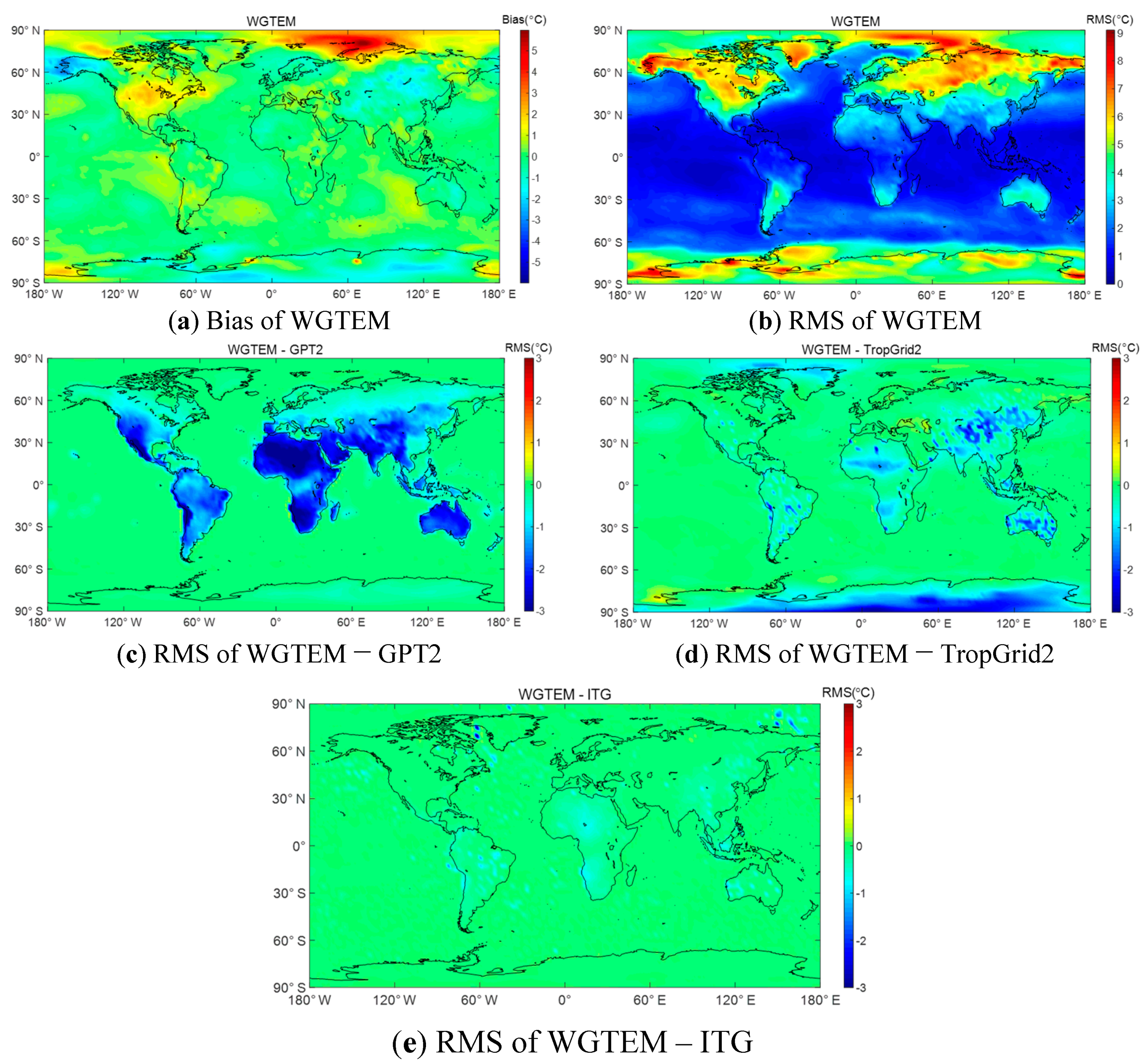
Figure 1 shows the global distribution of WGTEM temperature accuracy and global RMS differences with respect to other models, where a negative value indicates a higher accuracy. The figure shows that the accuracy at low latitudes was superior to that at high latitudes, and the accuracy for marine areas was higher than for land areas. It can also be seen from Figure 1c that the WGTEM accuracy in land areas was greatly improved compared to GPT2 (by over 2 °C). The most significant RMS improvement is seen in Africa, i.e., the Sahara Desert with a maximum value of 4.16 °C. For marine areas, the WGTEM model results were comparable with those of GPT2, and this was due to the stable diurnal temperature difference in marine areas. WGTEM also considered diurnal variations in temperature, whereas GPT2 did not. Therefore, WGTEM was more accurate than GPT2 for land areas. Although TropGrid2 concerned the diurnal variations and believed that the daily amplitude and the peak time of diurnal variation terms have annual periodic variation, it ignored the semi-annual periodic variation in temperature, which may cause deviations when estimating other periodic item coefficients. It is also evident from Figure 1d that TropGrid2 was less accurate than WGTEM for certain land areas, including most of the Antarctic region and part of the Arctic region (the RMS difference is 2.90 °C). This fact is mainly due to the obvious semi-annual periodic variation in temperature caused by the polar day and polar night phenomena in the Arctic. Moreover, it is worth mentioning that the TropGrid2 model was less accurate than GPT2 in most of the Arctic and Antarctic areas. In addition, WGTEM was more accurate in some areas than the ITG model.
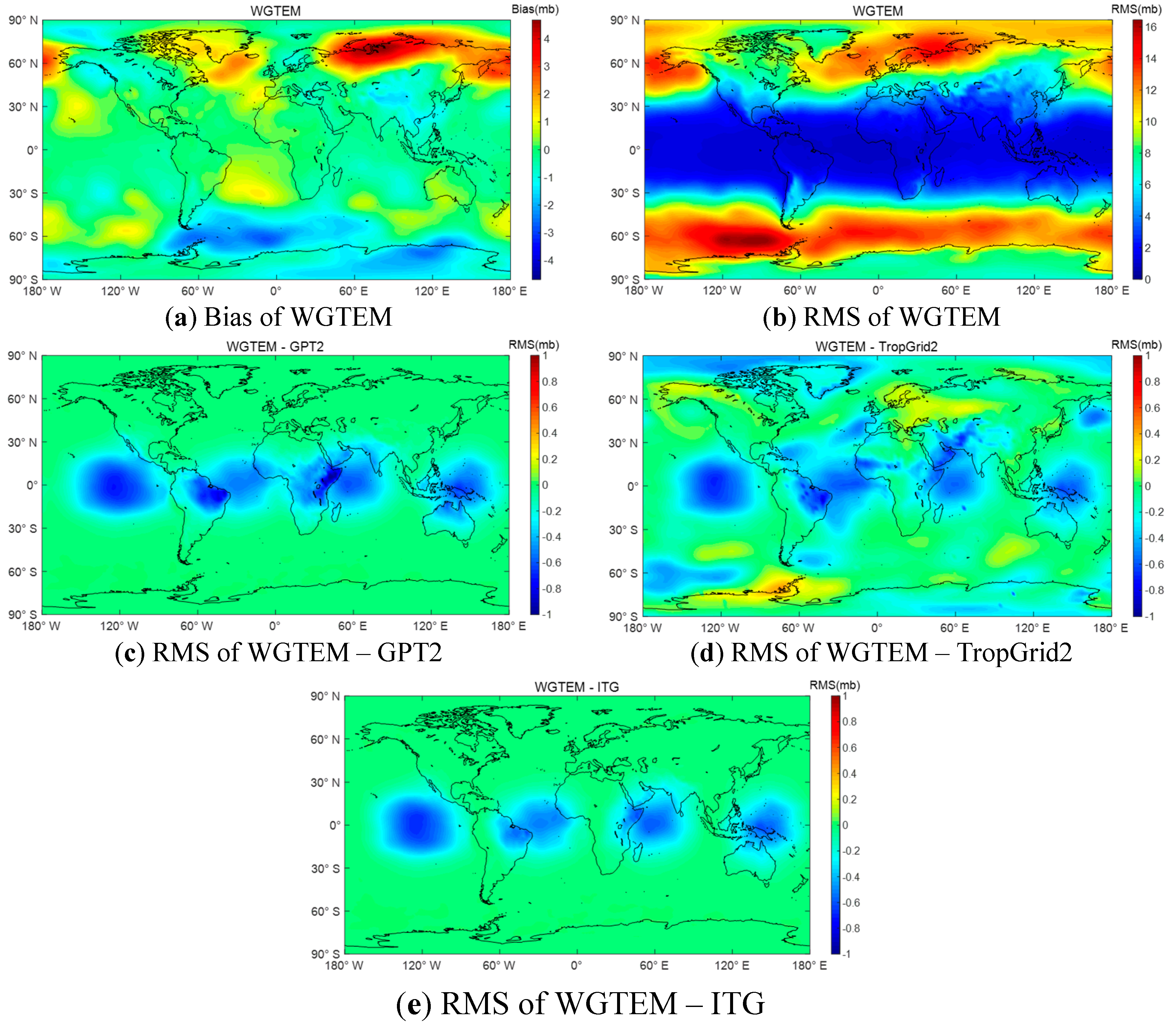
For the re-established air pressure model, statistical results with respect to the ECMWF reference are shown in Table 2. The global distribution of WGTEM air pressure accuracy and RMS differences are shown in Figure 2.
From Table 2, it can be revealed that the biases of all models were very similar, while the mean RMS value (6.95 mb) of WGTEM was the smallest and that of TropGrid2 (7.10 mb) was the largest. Figure 2 shows the overall trend in the WGTEM model’s air pressure accuracy, which demonstrates that it decreased with a rise in latitude. WGTEM improved the air pressure accuracy over GPT2 at the equator, with a maximum RMS improvement of 0.97 mb. Since it had the largest solar elevation angle close to the equator, the diurnal variation in air pressure was the most obvious, due to the effect of the sun: Therefore, the highest improvement with the WGTEM model was seen at the equator and its surrounding areas. Figure 2d displays that the WGTEM not only outperformed the TropGrid2 model at the equator, but also provided improved accuracy in the Arctic and Antarctic regions, with a maximum RMS improvement of 0.85 mb. TropGrid2 was less accurate than the other three models around the globe because it ignored the semi-annual periodic variation. The WGTEM model also had a superior air pressure accuracy over the ITG model at the equator, with a maximum RMS improvement of 0.68 mb. It is worth mentioning that there were two peaks and valleys in the daily variation of air pressure; but, the diurnal variation items of TropGrid2 and ITG can only reflect the changes in peak and valley once. Nonetheless, WGTEM can reflect two peaks and valleys in the daily variation of air pressure, which is consistent with the actual air pressure pattern. Therefore, the WGTEM model was more highly accurate in the term of air pressure.
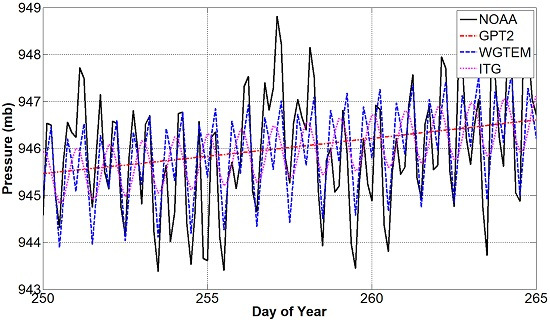
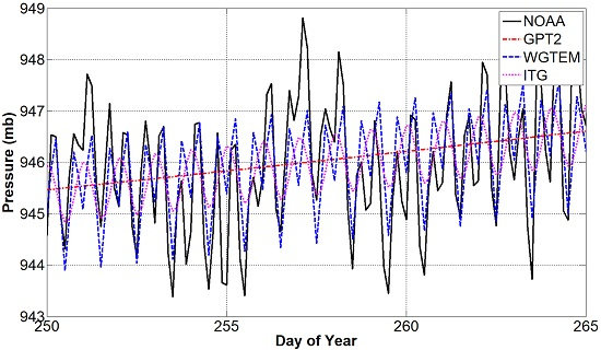
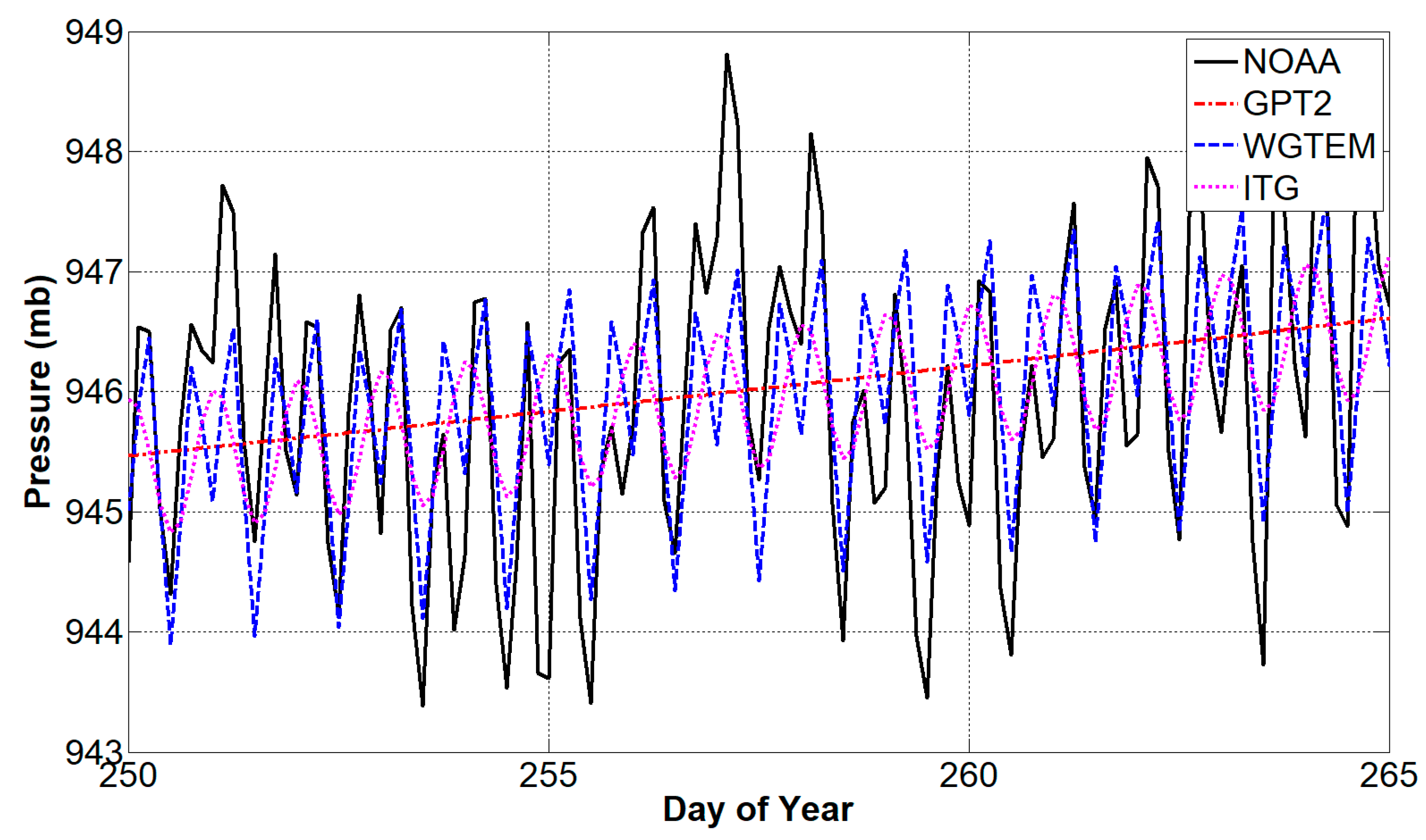
NOAA provides surface hourly/sub-hourly meteorological data for many stations globally. The air pressure at the meteorological station in Begumpet of day of year (DOY) 250–265 in 2012 was selected for analysis (see Figure 3), and the air pressure value was calculated for the same location and time using the WGTEM and GPT2 model.
Figure 3 displays the double-peak air pressure pattern during the daytime. The GPT2 model can only reflect the overall trend of this period and ITG can only reflect the single peak and valley. In contrast, WGTEM can show the double peaks and valleys of daily air pressure. Therefore, the performance of the WGTEM model expression was superior to that of GPT2, TropGrid2, and ITG.
3.2. External Accuracy Evaluation of WGTEM
To further analyze the validity, applicability, and superiority of the developed WGTEM model, this section validates the WGTEM’s accuracy using external data sources as references, including NOAA meteorological measurements and IGS final ZTD products. As the ITG model had already been proven to be more accurate than the GPT2 and the TropGrid2 models (Yao et al., 2015), the following section only focuses on a comparison between the WGTEM and ITG models.
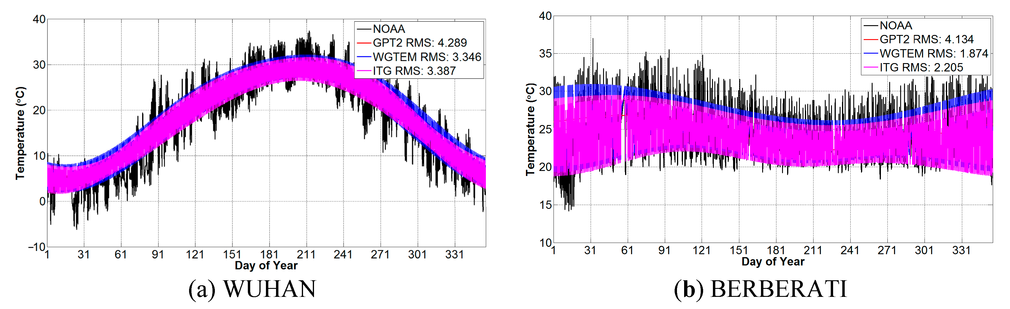
Two IGS Station located in Wuhan China and BERBERATI in Africa were selected to analyze the temperature provided by each model in 2012, as shown in Figure 4.
As can be seen from Figure 4, the WGTEM model’s accuracy is 3.3 °C at Wuhan station, which is comparable with that of ITG. Both values are larger than GPT2 by 1 °C. At BERBERATI station, the WGTEM accuracy reaches 1.9 °C, whereas that of ITG is 2.2 °C and GPT2 is 4.1 °C: Therefore, the WGTEM has an 18% and 21% accuracy improvement over ITG and GPT2, respectively.
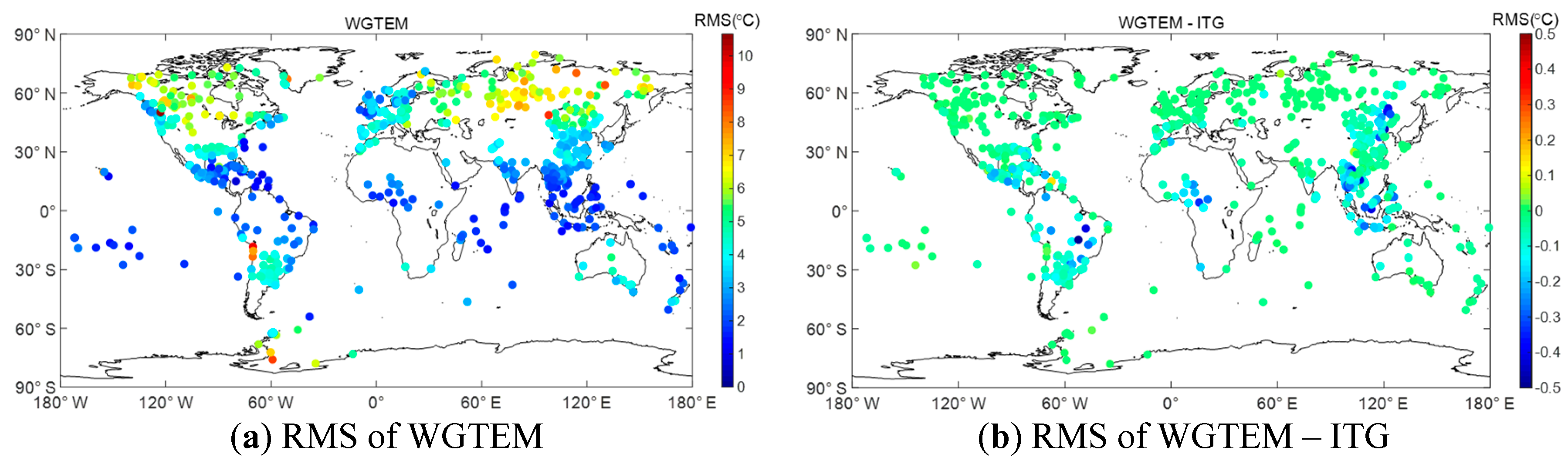
Next, we verify the WGTEM and ITG temperatures using NOAA data from 698 globally distributed meteorological stations in 2012 as a reference, and the statistical results are summarized in Table 3. Figure 5 shows the RMS of each station and the global distribution of temperature RMS differences between the WGTEM and ITG models.
Table 3 shows that the mean RMS of WGTEM at 698 stations was 3.81 °C and the bias was −0.26 °C; therefore, its accuracy was slightly better than that of ITG model. Figure 5 clearly shows that WGTEM temperature accuracy was highly related to latitude: The accuracy in low-latitude areas was evidently higher than that in high-latitude areas. Although the ITG model already considered the various periodic characteristics of temperature, WGTEM provided superior accuracy at some stations, with a maximum improvement of over 0.5 °C.
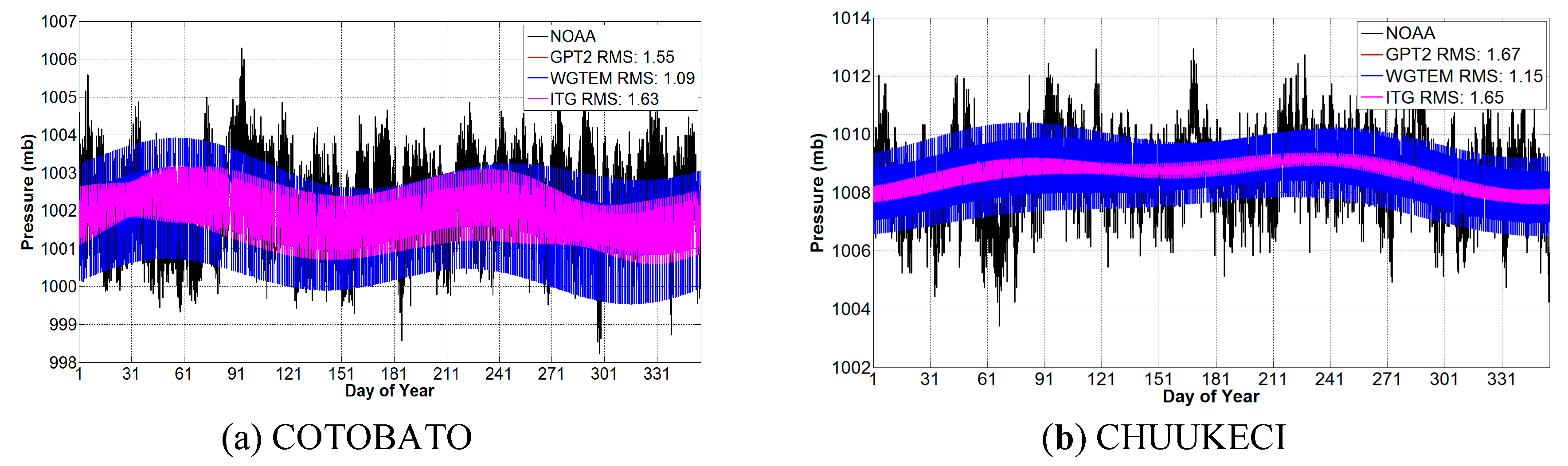
To analyze the air pressure accuracy, the COTOBATO station in the Philippines and the CHUUKECI station in Pacific Ocean were selected. Their air pressure series changes in 2012 are shown in Figure 6. The figure shows that the annual WGTEM RMS accuracy was 1.09 hPa at COTOBATO station, whereas that of GPT2 and ITG were 1.55 hPa and 1.63 hPa, respectively. In a word, WGTEM had the highest accuracy at this station. In addition, the ITG model was less accurate than GPT2, which is probably because the ITG did not consider the double-peak characteristics of air pressure. The annual RMS for WGTEM was 1.15 hPa at CHUUKECI station, whereas that of GPT2 and ITG was 1.67 hPa and 1.65 hPa, respectively. WGTEM was therefore still the most accurate model, and the accuracies of the ITG and GPT2 model were similar to each other.
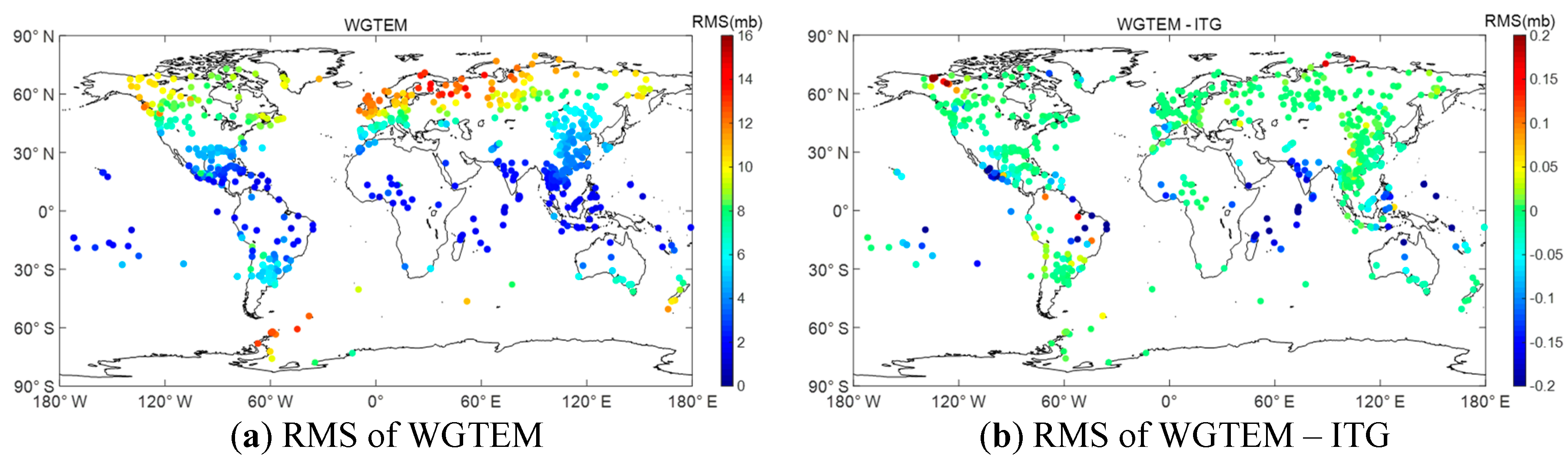
The air pressure comparison results are provided in Table 4 and Figure 7. The results in Table 4 show that the WGTEM model gave the optimal performance, with a mean/maximum/minimum bias of −0.2/7.8/−8.3 hPa, respectively. As for RMS, the mean value was 5.9 hPa, the maximum was 14.5 hPa, and the minimum was 1.1 hPa. Figure 7 shows the pattern of WGTEM air pressure is the same as that for temperature. To be specific, the accuracy decreased gradually with ascending latitude, and the accuracy at the equator reached 1.1 hPa. In addition, the model’s accuracy decreased significantly to 14.5 hPa in the Arctic owing to the dramatic dynamic change in air pressure. The negative difference between WGTEM and ITG shows that the WGTEM model was more accurate than the ITG. It is also clear that the WGTEM model’s accuracy was better than that of the ITG at some stations in the middle and low latitudes, with a maximum improvement of about 0.5 hPa.
Finally, the accuracy of WGTEM ZTD was analyzed and compared with that of the ITG model. One-year ZTD products for 274 IGS stations with a 1-h time resolution were selected, and the statistical results are listed in Table 5. Figure 8 depicts the RMS global distribution map for the WGTEM’s ZTDs at all stations as well as the differences between the results and ZTD RMS of the ITG model.
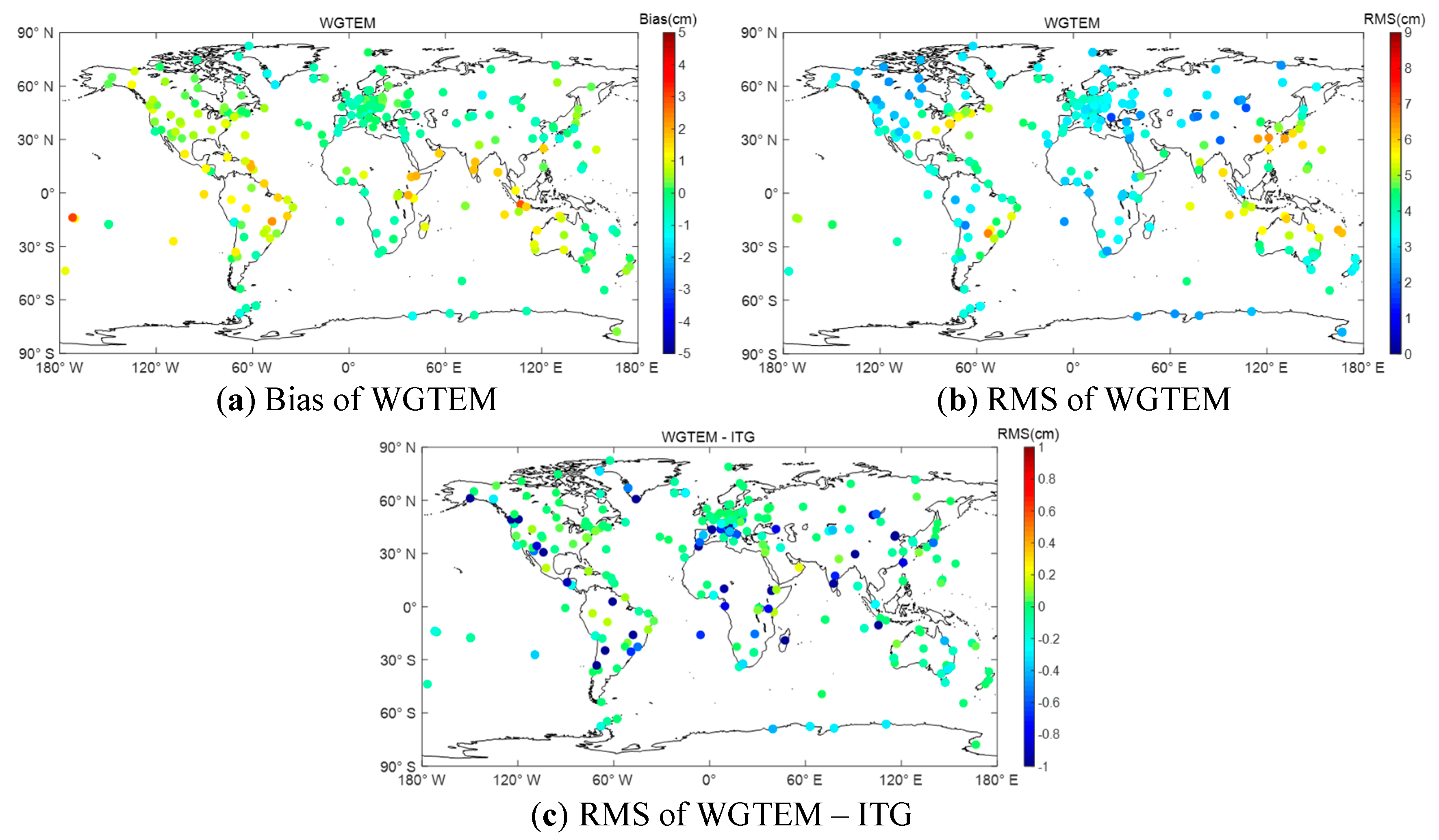
From Table 5, it is evident that the mean/maximum/minimum bias value of WGTEM ZTDs was 0.18/3.07/1.54 cm, respectively. The mean value of 274 for the RMS was 3.82 cm. In contrast, the mean bias of the ITG model was 0.05 cm, and the mean RMS value was 4.04 cm.
The WGTEM global bias map is shown in Figure 8a, where a positive bias indicates that the actual value was larger than empirical value and vice versa. It can be clearly seen from the figure that most stations with positive biases were located at the equator. As the highest ZHD accuracy was identified at the equator, it could be inferred that the mean empirical ZWD value is smaller than the actual value in 2012. The WGTEM global RMS map is depicted in Figure 8b. The WGTEM model had the highest accuracy in Europe, where the RMS of most stations was less than 4 cm. However, the accuracies of stations located in Asia, the east coast of the United States, and northern Australia were relatively low, with RMS values larger than 6 cm. The analysis of the ITG model in 2012 was similar to the RMS global distribution map. The differences were that the ITG model was built on ECWMF ERA-interim data, which have different accuracies in different regions around the world. A comparison between the RMS figures of WGTEM and ITG shows that the accuracy of WGTEM was superior at many stations, by a maximum of 3 cm. The accuracy was also comparatively improved at 20 stations by more than 1 cm, and by more than 0.5 cm at 47 stations. These results indicate that the WGTEM model expression was greatly improved compared to that of the ITG, with respect to ZTD.
In summary, the superiority of the WGTEM model expression makes it more accurate than the other three models described in Section 2. With the rise in accuracy and temporal resolution of data sources in the future, the WGTEM model’s accuracy will be accordingly improved due to the application of piecewise modeling.
4. Conclusions
The accuracy of tropospheric empirical model key parameters is highly reliant on the model expression and the modeling data sources employed. To ensure compatibility with high temporal resolution data sources in the future, this study proposes a new global tropospheric correction model, WGTEM, which is based on piecewise modeling. The WGTEM model expressions were evaluated using ERA-Interim and NOAA data.
Results show that the WGTEM model expressions are more accurate than the existing models including GPT2 Series Model, TropGrid2, and ITG. The external accuracy of the WGTEM model was then verified using NOAA meteorological measurements and IGS final ZTD products, and the results show that the accuracies of WGTEM temperature and air pressure are both better than those of the ITG model. At last, the ZTD accuracy was verified using IGS tracking station data, and results show that the ZTD expression of the WGTEM model is better than that of the ITG model. In addition, the mean bias and RMS of ZTD were 0.18 cm and 3.82 cm, respectively. The enhancement of the WGTEM model expression makes it more accurate than ITG model. The ITG model has an annual period term, a semi-annual period, and a daily period term, but the temporal resolution of its daily period term is very low. The temporal resolution of the ITG model is limited, and its accuracy will not increase with the temporal resolution of the modeling data sources employed. Compared with ITG, the accuracy of WGTEM can be improved mainly due to its self-adaptive temporal resolution.
When the temporal resolution of the modeling data source is improved in the future, the temporal resolution and accuracy of WGTEM can be further improved. It is also anticipated that with future improvements in the precision and temporal resolution of data sources, the accuracy and temporal resolution of WGTEM model will also steadily increase. Any reader can update the WGTEM model coefficients with new available data.
Author Contributions
Data curation, W.P.; formal analysis, Y.Y.; investigation, C.X.; methodology, Q.Z.; software, J.S.; validation, C.X.; writing—original draft, J.B.; writing—review and editing, C.X. All authors have read and agreed to the published version of the manuscript.
Funding
This research was supported by the National Natural Science Foundation of China (Nos. 41721003, 41874033, 41804038 and 41604002).
Acknowledgements
The authors would like to thank ECMWF and NOAA for providing experimental data.
Conflicts of Interest
The authors declare no conflict of interest.
References
- Rocken, C.; Van Hove, T.; Ware, R. Near real—Time GPS sensing of atmospheric water vapor. Geophys. Res. Lett. 1997, 24, 3221–3224. [Google Scholar] [CrossRef] [Green Version]
- Allan, R.P. The role of water vapour in Earth’s energy flows. Surv. Geophys. 2012, 33, 557–564. [Google Scholar] [CrossRef] [Green Version]
- Bevis, M.; Businger, S.; Chiswell, S.; Herring, T.A.; Anthes, R.A.; Rocken, C.; Ware, R.H. GPS meteorology: Mapping zenith wet delays onto precipitable water. J. Appl. Meteorol. 1994, 33, 379–386. [Google Scholar] [CrossRef]
- Duan, J.; Bevis, M.; Fang, P.; Bock, Y.; Chiswell, S.; Businger, S.; McClusky, S. GPS meteorology: Direct estimation of the absolute value of precipitable water. J. Appl. Meteorol. Clim. 1996, 35, 830–838. [Google Scholar] [CrossRef] [Green Version]
- Jacob, D. The role of water vapour in the atmosphere. A short overview from a climate modeller’s point of view. Phys. Chem. Earth Part A Solid Earth Geod. 2001, 26, 523–527. [Google Scholar] [CrossRef]
- Cai, C.; Gao, Y. Precise point positioning using combined GPS and GLONASS observations. Positioning 2007, 1, 13–22. [Google Scholar] [CrossRef] [Green Version]
- Collins, P.; Lahaye, F.; Héroux, P.; Bisnath, S. Precise point positioning with ambiguity resolution using the decoupled clock model. In Proceedings of the 21st international technical meeting of the satellite division of the Institute of Navigation (ION GNSS 2008), Savannah, GA, USA, 16–19 September 2008. [Google Scholar]
- Li, X.; Ge, M.; Zhang, H.; Wickert, J. A method for improving uncalibrated phase delay estimation and ambiguity-fixing in real-time precise point positioning. J. Geod. 2013, 87, 405–416. [Google Scholar] [CrossRef]
- Li, X.; Ge, M.; Dai, X.; Ren, X.; Fritsche, M.; Wickert, J.; Schuh, H. Accuracy and reliability of multi-GNSS real-time precise positioning: GPS, GLONASS, BeiDou, and Galileo. J. Geod. 2015, 89, 607–635. [Google Scholar] [CrossRef]
- Lu, C.; Zus, F.; Ge, M.; Heinkelmann, R.; Dick, G.; Wickert, J.; Schuh, H. Tropospheric delay parameters from numerical weather models for multi-GNSS precise positioning. Atmos. Meas. Tech. 2016, 9, 5965. [Google Scholar] [CrossRef] [Green Version]
- Hopfield, H.S. Two-quartic Tropospheric Refractivity Profile for Correcting Satellite Data. J. Geophys. Res. 1969, 74, 4487–4499. [Google Scholar] [CrossRef]
- Saastamoinen, J. Atmospheric correction for the troposphere and stratosphere in radio ranging satellites. Use Artif. Satell. Geod. 1972, 15, 247–251. [Google Scholar]
- Ifadis, I. The Atmospheric Delay of Radio Waves: Modelling the Elevation Dependence on a Global Scale; Technical Report No. 38L; School of Electrical and Computer Engineering, Chalmers University of Technology: Goteburg, Sweden, 1986. [Google Scholar]
- Askne, J.; Nordius, H. Estimation of Tropospheric Delay for Microwaves from Surface Weather Data. Radio Sci. 1987, 22, 379–386. [Google Scholar] [CrossRef]
- Wang, G.Q. Millimeter-accuracy GPS landslide monitoring using Precise Point Positioning with Single Receiver Phase Ambiguity (PPP-SRPA) resolution: A case study in Puerto Rico. J. Geod. Sci. 2013, 3, 22–31. [Google Scholar] [CrossRef]
- Rabbou, M.A.; El-Rabbany, A. PPP accuracy enhancement using GPS/GLONASS observations in kinematic mode. Positioning 2015, 6, 1–6. [Google Scholar] [CrossRef] [Green Version]
- Maciuk, K. GPS-only, GLONASS-only and combined GPS + GLONASS absolute positioning under different sky view conditions. Tehnički Vjesnik 2018, 25, 933–939. [Google Scholar]
- Ge, Y.; Dai, P.; Qin, W.; Yang, X.; Zhou, F.; Wang, S.; Zhao, X. Performance of multi-GNSS precise point positioning time and frequency transfer with clock modeling. Remote Sens. 2019, 11, 347. [Google Scholar] [CrossRef] [Green Version]
- Wu, Q.; Sun, M.; Zhou, C.; Zhang, P. Precise point positioning using dual-frequency GNSS observations on smartphone. Sensors 2019, 19, 2189. [Google Scholar] [CrossRef] [Green Version]
- Shi, J.; Gao, Y. A troposphere constraint method to improve PPP ambiguity-resolved height solution. J. Navig. 2014, 67, 249–262. [Google Scholar] [CrossRef]
- Shi, J.; Xu, C.; Guo, J.; Gao, Y. Local troposphere augmentation for real-time precise point positioning. Earth Planets Space 2014, 66, 30. [Google Scholar] [CrossRef] [Green Version]
- Collins, J.P.; Langley, R.B. A Tropospheric Delay Model for the User of the Wide Area Augmentation System; Department of Geodesy and Geomatics Engineering, University of New Brunswick: Fredericton, NB, Canada, 1997. [Google Scholar]
- Collins, J.P.; Langley, R. The residual tropospheric propagation delay: How bad can it get? Proceedings of Ion GPS; Institute of Navigation: Manassas, VA, USA, 1998; Volume 11, pp. 729–738. [Google Scholar]
- Penna, N.; Dodson, A.H.; Chen, W. Assessment of EGNOS Tropospheric Correction Model; ION GPS: Nashville, TN, USA, 1999; pp. 14–17. [Google Scholar]
- Penna, N.; Dodson, A.; Chen, W. Assessment of EGNOS tropospheric correction model. J. Navig. 2001, 54, 37–55. [Google Scholar] [CrossRef] [Green Version]
- Ueno, M.; Hoshinoo, K.; Matsunaga, K.; Kawai, M.; Nakao, H.; Langley, R.B.; Bisnath, S.B. Assessment of atmospheric delay correction models for the Japanese MSAS. In Proceedings of the 14th International Technical Meeting of the Satellite Division of The Institute of Navigation, Salt Lake City, UT, USA, 11–14 September 2001; pp. 2341–2350. [Google Scholar]
- Krueger, E.; Schueler, T.; Hein, G.W.; Martellucci, A.; Blarzino, G. Galileo Tropospheric Correction Approaches Developed within GSTB-V1. Proceedings of ENC-GNSS 2004, Rotterdam, The Netherlands, 16–19 May 2004; Available online: https://www.researchgate.net/profile/Torben_Schueler/publication/228730717_Galileo_Tropospheric_Correction_Approaches_Developed_within_GSTB-V1/links/09e4150880fbbbaca7000000/Galileo-Tropospheric-Correction-Approaches-Developed-within-GSTB-V1.pdf (accessed on 14 February 2020).
- Schüler, T. The TropGrid2 standard tropospheric correction model. GPS Solut. 2014, 18, 123–131. [Google Scholar] [CrossRef]
- Böhm, J.; Heinkelmann, R.; Schuh, H. Short note: A global model of pressure and temperature for geodetic applications. J. Geod. 2007, 81, 679–683. [Google Scholar] [CrossRef]
- Kouba, J. Testing of Global Pressure/Temperature (GPT) Model and Global Mapping Function (GMF) in GPS analyses. J. Geod. 2009, 83, 199–208. [Google Scholar] [CrossRef]
- Lagler, K.; Schindelegger, M.; Boehm, J.; Krasna, H.; Nilsson, T. GPT2: Empirical slant delay model for radio space geodetic techniques. Geophys. Res. Lett. 2013, 40, 1069–1073. [Google Scholar] [CrossRef] [Green Version]
- Böhm, J.; Möller, G.; Schindelegger, M.; Pain, G.; Weber, R. Development of an improved empirical model for slant delays in then troposphere (GPT2w). GPS Solut. 2015. [Google Scholar] [CrossRef] [Green Version]
- Yao, Y.; Xu, C.; Shi, J.; Cao, N.; Zhang, B.; Yang, J. ITG: A new global GNSS tropospheric correction model. Sci. Rep. 2015, 5, 10273. [Google Scholar] [CrossRef] [Green Version]
Figure 1.
Global distribution of temperature accuracy for Wuhan-University Global Tropospheric Empirical Model (WGTEM) and global RMS differences with reference to other models, validated by ECMWF data.
Figure 1.
Global distribution of temperature accuracy for Wuhan-University Global Tropospheric Empirical Model (WGTEM) and global RMS differences with reference to other models, validated by ECMWF data.

Figure 2.
Global distribution of air pressure accuracy for WGTEM and global RMS differences with other models, validated by ECMWF data.
Figure 2.
Global distribution of air pressure accuracy for WGTEM and global RMS differences with other models, validated by ECMWF data.

Figure 3.
Air pressure time series from National Oceanic and Atmospheric Administration (NOAA) and three models at meteorological station in Begumpet during day of year (DOY) 250–264 in 2012.
Figure 3.
Air pressure time series from National Oceanic and Atmospheric Administration (NOAA) and three models at meteorological station in Begumpet during day of year (DOY) 250–264 in 2012.

Figure 4.
Temperature series in 2012 from NOAA, GPT2 model, WGTEM, and Improved Tropospheric Grid (ITG) model at two International GNSS Service (IGS) stations.
Figure 4.
Temperature series in 2012 from NOAA, GPT2 model, WGTEM, and Improved Tropospheric Grid (ITG) model at two International GNSS Service (IGS) stations.

Figure 5.
Temperature RMS from WGTEM at each station, and comparison of global temperature RMS differences between ITG model and WGTEM validated by NOAA data.
Figure 5.
Temperature RMS from WGTEM at each station, and comparison of global temperature RMS differences between ITG model and WGTEM validated by NOAA data.

Figure 6.
Air pressure time series changes at Chuukeci and Cotobato Stations in 2012 from NOAA, and comparison between GPT2 model, WGTEM, and ITG model results for both stations.
Figure 6.
Air pressure time series changes at Chuukeci and Cotobato Stations in 2012 from NOAA, and comparison between GPT2 model, WGTEM, and ITG model results for both stations.

Figure 7.
Air pressure RMS from WGTEM at each station, and comparison with RMS from ITG model, validated by NOAA data.
Figure 7.
Air pressure RMS from WGTEM at each station, and comparison with RMS from ITG model, validated by NOAA data.

Figure 8.
ZTD bias and RMS from WGTEM at each station and comparison with RMS from ITG model, validated by NOAA data.
Figure 8.
ZTD bias and RMS from WGTEM at each station and comparison with RMS from ITG model, validated by NOAA data.


Table 1.
Root Mean Square (RMS) of temperature results from different models validated by European Centre for Medium-range Weather Forecasts (ECMWF) data.
Table 1.
Root Mean Square (RMS) of temperature results from different models validated by European Centre for Medium-range Weather Forecasts (ECMWF) data.
| Model | RMS (°C) | ||
|---|---|---|---|
| Mean | Max | Min | |
| GPT2 | 3.20 | 9.32 | 0.46 |
| TropGrid2 | 3.11 | 9.07 | 0.47 |
| ITG | 2.89 | 9.11 | 0.44 |
| WGTEM | 2.85 | 9.10 | 0.43 |
Table 2.
RMS of air pressure results from different models validated by ECMWF data.
| Model | RMS (mb) | ||
|---|---|---|---|
| Mean | Max | Min | |
| GPT2 | 7.04 | 16.45 | 0.82 |
| TropGrid2 | 7.10 | 16.63 | 0.77 |
| ITG | 7.03 | 16.40 | 0.78 |
| WGTEM | 6.95 | 16.45 | 0.75 |
Table 3.
Bias and RMS of temperature statistics from WGTEM and ITG models validated by NOAA data.
| Model | Bias (°C) | RMS (°C) | ||||
|---|---|---|---|---|---|---|
| Mean | Max | Min | Mean | Max | Min | |
| WGTEM | −0.26 | 6.86 | −9.14 | 3.81 | 10.66 | 0.67 |
| ITG | −0.27 | 6.84 | −9.14 | 3.87 | 10.66 | 0.69 |
Table 4.
Bias and RMS of air pressure results from different models validated by NOAA data.
| Model | Bias (hPa) | RMS (hPa) | ||||
|---|---|---|---|---|---|---|
| Mean | Max | Min | Mean | Max | Min | |
| WGTEM | −0.2 | 7.8 | −8.3 | 5.9 | 14.5 | 1.1 |
| ITG | −0.2 | 7.8 | −8.3 | 6.0 | 14.6 | 1.4 |
Table 5.
Bias and RMS of Zenith Tropospheric Delay (ZTD) results from WGTEM and ITG models validated by IGS ZTD products.
Table 5.
Bias and RMS of Zenith Tropospheric Delay (ZTD) results from WGTEM and ITG models validated by IGS ZTD products.
| Model | ZTD Bias (cm) | ZTD RMS(cm) | ||||
|---|---|---|---|---|---|---|
| Mean | Max | Min | Mean | Max | Min | |
| WGTEM | 0.18 | 3.07 | −1.54 | 3.82 | 6.62 | 1.65 |
| ITG | 0.05 | 4.71 | −4.57 | 4.04 | 6.62 | 1.70 |
© 2020 by the authors. Licensee MDPI, Basel, Switzerland. This article is an open access article distributed under the terms and conditions of the Creative Commons Attribution (CC BY) license (http://creativecommons.org/licenses/by/4.0/).
Share and Cite
MDPI and ACS Style
Xu, C.; Yao, Y.; Shi, J.; Zhang, Q.; Peng, W. Development of Global Tropospheric Empirical Correction Model with High Temporal Resolution. Remote Sens. 2020, 12, 721. https://0-doi-org.brum.beds.ac.uk/10.3390/rs12040721
AMA Style
Xu C, Yao Y, Shi J, Zhang Q, Peng W. Development of Global Tropospheric Empirical Correction Model with High Temporal Resolution. Remote Sensing. 2020; 12(4):721. https://0-doi-org.brum.beds.ac.uk/10.3390/rs12040721
Chicago/Turabian StyleXu, Chaoqian, Yibin Yao, Junbo Shi, Qi Zhang, and Wenjie Peng. 2020. "Development of Global Tropospheric Empirical Correction Model with High Temporal Resolution" Remote Sensing 12, no. 4: 721. https://0-doi-org.brum.beds.ac.uk/10.3390/rs12040721
Note that from the first issue of 2016, this journal uses article numbers instead of page numbers. See further details here.