Extraction of Yardang Characteristics Using Object-Based Image Analysis and Canny Edge Detection Methods


1
School of Earth Sciences, China University of Geosciences, Wuhan 430074, China
2
Guangdong Provincial Key Laboratory of Marine Biotechnology, Institute of Marine Sciences, Shantou University, Shantou 515063, China
3
College of Geology Engineering and Geomatics, Chang’an University, Xi’an 710054, China
4
School of Geodesy and Geomatics, Wuhan University, Wuhan 430074, China
*
Author to whom correspondence should be addressed.
Remote Sens. 2020, 12(4), 726; https://0-doi-org.brum.beds.ac.uk/10.3390/rs12040726
Submission received: 31 December 2019
/
Revised: 18 February 2020
/
Accepted: 20 February 2020
/
Published: 22 February 2020
(This article belongs to the Special Issue Remote Sensing of Dryland Environment)
Abstract
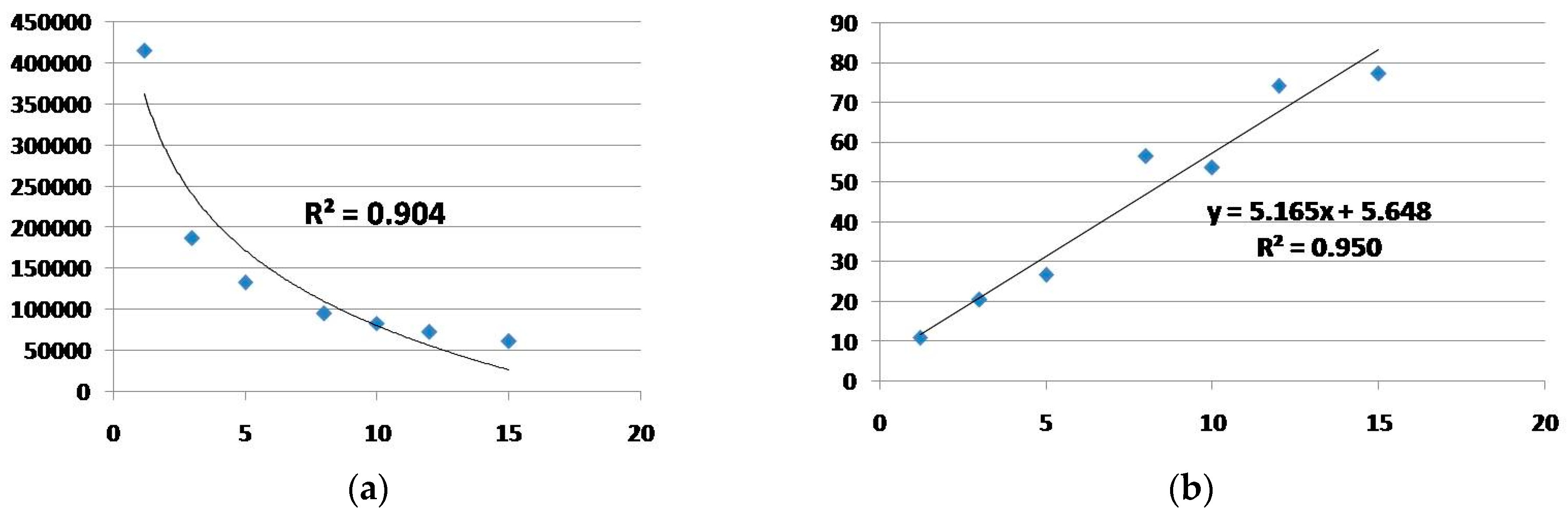
:Parameters of geomorphological characteristics are critical for research on yardangs. However, methods which are low-cost, accurate, and automatic or semi-automatic for extracting these parameters are limited. We present here semi-automatic techniques for this purpose. They are object-based image analysis (OBIA) and Canny edge detection (CED), using free, very high spatial resolution images from Google Earth. We chose yardang fields in Dunhuang of west China to test the methods. Our results showed that the extractions registered an overall accuracy of 92.26% with a Kappa coefficient of agreement of 0.82 at a segmentation scale of 52 using the OBIA method, and the exaction of yardangs had the highest accuracy at medium segmentation scales (138, 145). Using CED, we resampled the experimental image subset to a series of lower spatial resolutions for eliminating noise. The total length of yardang boundaries showed a logarithmically decreasing (R2 = 0.904) trend with decreasing spatial resolution, and there was also a linear relationship between yardang median widths and spatial resolutions (R2 = 0.95). Despite the difficulty of identifying shadows, the CED method achieved an overall accuracy of 89.23% with a kappa coefficient of agreement of 0.72, similar to that of the OBIA method at medium segmentation scale (138).
1. Introduction
Yardangs are wind-eroded ridges that develop at a range of scales, from meters to kilometers in length, and meters to tens of meters in height [1,2]. They originate from a number of formative processes, including wind abrasion, deflation, fluvial erosion, mass movements, and weathering [2,3,4,5,6,7,8]. Abrasion is the most important process in shaping yardangs [7], while deflation may be important in the evolution of yardangs found in less indurated lacustrine material [8]. Temporary runoff may accelerate the formation of yardangs during the initial stages of their development [8]. Mega-yardangs are distributed in Central Asia, western Afghanistan, Lut Desert of southern Iran, Western Desert of Egypt etc., and they tend to occur in relatively homogeneous rocks, sites of active dune accumulation, and in hyper-arid and trade wind areas [4].
Since the 1900s, researchers have conducted numerous studies on the distributions [4,9], definitions [10,11,12,13], morphological characteristics [7,9,14,15,16], formation ages [15,17,18], and formative processes [19,20,21,22,23] of yardang landforms in different locations.
With the advance of remote sensing, we can obtain more information about yardangs: (1) Different yardang landforms have been found on other planets, such as Mars [24,25,26], Titan [27], and Venus [24,25,26]; (2) new methods can be used to investigate the characteristics of yardangs, such as unmanned aerial vehicles [23,28], very high-resolution images from Google Earth [14], photogrammetry and GIS (Geographic Information System) technologies [29].
Geomorphological characteristic parameters (e.g., area, length, width, length/width ratio, long-axis strike, etc.) are critical factors for yardang research. As a kind of wind erosion landform, the long-axis strike of yardangs always aligns with the prevailing wind direction and can be used to reconstruct the local wind direction [30]. A teardrop shape that approaches an ideal 1:4 length/width (l/w) ratio based on aerodynamic considerations represents a mature stage of yardang evolution [7]. Hu et al. [14] classified yardangs into four types, while Wang et al. [23] classified yardangs into 11 types out of four main groups based on their l/w ratios and morphologies, in Qaidam basin.
Previous researchers usually calculated these yardang parameters using field surveys [30,31]. Studies on yardangs have increasingly benefitted from remote sensing techniques, such as photographic surveys [29,32], manual extraction from very high-resolution images from Google Earth [14,16] and UAV(unmanned aerial vehicle) images [23,28]. However, these methods are costly and inefficient. Recently, some researchers have focused on automatic or semi-automatic methods for the extraction of yardangs. Ehsani and Quiel [33] characterized yardangs using self-organizing maps and SRTM (Shuttle Radar Topography Mission) data. They showed that all yardangs were clearly recognized when their widths were larger than the spatial resolution of DEM (Digital Elevation Model) data (90 m/pix) and that most terrestrial yardangs’ widths are smaller than the free-access DEM’s resolution (30/90 m/pix). The ellipse-fitting method can be used for calculating the morphological parameters of yardangs based on DEM extracted from UAV images [28]. The lengths of the long and short axes of the fitted ellipses represent the length and width of yardangs, and the slope of the long axes represents the orientation of yardangs. But it is time-consuming and expensive for getting UAV images.
For the past 20 years, Object-based image analysis (OBIA) has represented a new paradigm in remote sensing and GIS science. An increasing number of empirical studies have demonstrated the advantages that OBIA methods offer over the traditional pixel-based methods [34]. OBIA is primarily applied for classifications of high (spatial) resolution images, and the main advantage is that a series of morphological, contextual, and textural characteristics of the input data can be effectively used [35,36]. OBIA has shown great potentials for the extraction of yardangs. Google Earth can offer free, large scale, and very high spatial resolution images [37], and provides a good data source for yardang mapping. Researchers can obtain ideal classification results by analyzing the spectral, textural, and geometrical features in very high-resolution images [38]. Yardangs always have several obvious features in very high-resolution images (Figure 1). They tend to be brighter than other objects and have regular shapes and specific directions. Yardangs have obvious textural features different from other objects due to their uneven surface, which can also be used for extraction.
The Canny edge detection algorithm [39] is widely used to locate sharp intensity changes and to detect object boundaries in an image [40]. Zhao et al. [28] first used it for acquiring the edge of yardangs in 15-m medium-resolution Landsat 8 OLI data. Images of 15-m spatial resolution may lead to low accuracy for the extraction of micro-yardangs.
Despite numerous descriptions of yardangs in Dunhuang of west China, extracting of yardang parameters is still limited. For example, Dong et al. [20] measured yardang attributes but did not describe the extraction method. Niu [29] calculated yardang parameters (area, perimeter, length, width, height, and long-axis direction) but based this on photogrammetry and GIS technologies.
We here seek to fill this important research niche by focusing on: (1) extraction of yardang parameters using a very high spatial resolution image subset in Google Earth based on OBIA and Canny edge detection (CED) methods; (2) discussing the relationship between segmentation scale, spatial image resolution, and yardang size.
2. Materials
2.1. The Study Area
The study area is located in the northwest of Dunhuang, Gansu Province, China, 160 km away from Dunhuang City [41], the northeast margin of Tibetian Plateau. It is characterized by a typical arid climate, with mean annual temperature and precipitation of 9.2 °C and 44.5 mm, respectively. The mean annual evaporation is 2444 mm [42]. The main landform types in the area are yardangs, black gobi in the corridors among yardangs, sand ripples, and dunes (barchans, transverse and linear sand dunes) [43].Yardangs have developed on interbedded strata of hard, cemented lacustrine/fluvial deposits and loose soft aeolian deposits [20]. The height of the yardangs ranges from 10 to 20 m, and length ranges from 10 to 1800 m, and their width ranges from 5 to 300 m [20].
2.2. Data
The very high spatial resolution image subset for this study was acquired in Google Earth. It was free downloaded using the website (www.91weitu.com). The image subset was captured in May 2016, only available in R (red) G (green) B (blue) bands (no sensor and bands information), with a resolution of 1.19 m. The projection used was the WGS 1984 Web Mercator Auxiliary Sphere. The image was re-projected to the UTM (Universal Transverse Mercator) Zone 46N system with WGS 1984 Datum, presenting an area of approximately 5.04 km2 (Figure 1).
3. Methods
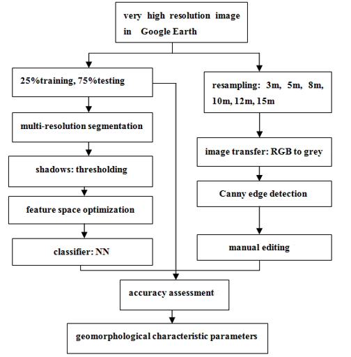
In our study, two methods (OBIA and CED) were used for extracting yardang parameters. For the OBIA method, the whole image subset was split into four parts, one part for training, and the others for testing. In this work, the eCognition software system was used to complete the OBIA classification. For the CED method, we first coarsened the image subset’s resolution to reduce image noise. The extraction process was completed in MATLAB 2016. Detailed classification and extraction steps are listed in (Figure 2).
3.1. OBIA Method
3.1.1. Image Segmentation
Image segmentation is the creation of image objects according to specific criteria. The multi-resolution segmentation algorithm was used in the study. It is a bottom-up region-merging technique starting with one-pixel objects and well used for detecting object boundaries [44]. The algorithm is controlled by three user-defined parameters: scale, shape, and compactness. The scale parameter determines the maximum standard deviation of heterogeneity for image objects. The higher is the value, the larger the generated image objects. The shape parameter defines the textural heterogeneity of the resulting image objects. If we wanted to make more use of spectral information, the shape value would have to be lower. The compactness value optimizes the image objects in regards to overall compactness and smoothing borders [45]. The values of shape and compactness parameters are on a scale (0, 1).
In our study, the yardangs had an obvious spectral difference from other objects, and the shapes of segmentation objects can reflect the original geometry of yardangs, so the shape parameter was set to 0.1 with less weight. The compactness parameter was set to 0.5, balancing compactness and smoothness.
ESP (estimation of scale parameter) is a tool to estimate scale parameter for multi-resolution image segmentation. The fundamental idea of this tool is in the following: multi-resolution segmentation is a bottom-up process in which objects are merged from small to large, and the criterion for merging is the heterogeneity of image objects. Local variance (LV) of image object heterogeneity can be expressed as the mean standard deviation of image objects at the same level. In general, with the increase of segmentation scale, LV will present a stable change process. On the contrary, when the segmentation scale is close to the optimal scale of ground objects, LV will have a large change. The rate of change of LV (ROC-LV) can well reflect this process, and the peaks of ROC-LV indicate the scales at which the image can be segmented [46].
where L = LV at the target level and L − 1 = LV at the next lower level, LV represents the pixels’ average variance of gray value in the image objects.
3.1.2. Shadow Detection
An obvious characteristic of yardang shadows is that their brightness values are significantly lower than those of other categories. Thus, it is easy to extract them using brightness information. We calculated the maximum brightness value of shadows in the training area, then used the thresholds to separate them from other objects.
There are two types of shadows: (1) true shadows next to the yardangs, (2) false shadows on the yardangs caused by the undulation of the surface, which should be classified as yardangs after accuracy assessment.
3.1.3. Object Features
Object features are the basis for image analysis and information extraction. One of the main advantages of OBIA is that a variety of spectral, textural, and geometric features can be extracted from segmented image objects and can be utilized in classification [47].
The spectral features refer to grey-level values in image bands. Common spectral features include meaning, standard deviation (SD), brightness, and maxdiff (see below). Mean and SD are the mean value and standard deviation of the pixel grey values for one object in each band. Brightness is the mean object grey value of all bands. Maxdiff represents the ratio of the maximum and minimum mean value difference to the brightness [48].
Textural features describe the spatial arrangements of grey-level values and spatial correlation among image objects [49]. The grey level co-occurrence matrix (GLCM) [50] is the most commonly used method for texture feature analysis. Main textural measures such as homogeneity (Hom), entropy (Ent), contrast (Con), mean, and standard deviation (Std) can be extracted based on GLCM [51]. As the alignment of yardangs in the study area was almost from north to south, we selected directions from 0° to 135° with 45° intervals (0° in the north), which were either parallel to or perpendicular to the alignment of yardangs for calculating textural features. All of them could be calculated in five ways depending on the directions: 0°, 45°, 90°, 135°, and all (summing up the four directional GLCM textures).
Geometric features mainly reflect the geometric parameters of the objects. A set of geometry features such as area, compactness, density, main direction, roundness, and shape index can be calculated. Compactness, density, and roundness are features used to measure the irregularity of the edge of the object. The shape index reflects the smoothness of the object boundary.
3.1.4. Feature Space Optimization
A separability and thresholds (SEaTH) algorithm [52] was used for the feature space optimization in our study. It is a statistical method based on training sample data. Jeffries–Matudita distance (J) on a scale [0, 2] measures the separability between classes. For two classes C1 and C2, the greater J measures, the better the separability. J can be computedfrom
and
where mi and (i = 1,2) respectively represent the mean and variance of a given feature for two classes.
3.1.5. Classification
In order to classify segmented image objects with their selected features determined by the aforementioned feature selection techniques, a nearest neighbor (NN) classifier was employed. NN classifier, one of the simplest algorithms, is a Euclidean distance-based algorithm, assigns an unlabelled image pixel (or object) the class label of its nearest neighboring pixels (or objects) in the feature space [47].
3.2. CED Method
High-resolution images contain a large amount of object information, but there are also a lot of noise (e.g., linear textures on yardangs and shadows around them) that affect the extraction accuracy. This noise cannot be eliminated easily by the conventional methods (expanding filter radius and increasing threshold). In this section, we proposed the CED method based on resampling to reduce noise and improve the efficiency of boundary extraction (Figure 2).
3.2.1. Resampling
Bilinear interpolation was applied for the resampling. This involves a linear interpolation by using pixel values of four adjacent points and assigning different weights according to their distance from the interpolation point [53]. This method has an average low-pass filtering effect, and the edges are smoothed to produce a coherent output image. The original image was resampled to six different spatial resolution images: 3 m, 5 m, 8 m, 10 m, 12 m, and 15 m.
3.2.2. RGB to Greyscale Transferring
As the CED method usually detects object boundaries using greyscale images, the RGB image should be converted into greyscale. A weighted average method was used to complete the image conversion [54]. The determination of band weights takes into account the physiological characteristics of human eyes. Human vision has the highest sensitivity to green, followed by red, and the lowest sensitivity to the blue [55]. The conversion formula is listed as follows
where Grey is the brightness of the pixel in the greyscale images, and R, G, B are brightness values of the red, green, and blue bands of the same pixel in color images.
3.2.3. Canny Edge Detection
The detection process consisted of four steps: (1) utilized a Gaussian filter to smooth the image and remove noise; (2) calculated the gradient amplitude and direction with the finite-difference of the first partial derivative at each pixel; (3) non-maximum suppressed the gradient amplitude; and (4), applied double thresholds to determine and connect potential edges [40,56].
3.2.4. Manual Editing
After the edge extraction was completed, we needed several steps of manual editing to acquire the accurate boundary of yardangs: (1) selected appropriately closed, U- and V-shaped yardang boundaries in different edge detection results achieved from different spatial resolution images using manual interpretation; (2) merged all of the boundaries together, selected one detected from higher resolution image if the boundaries overlapped; (3) connected breakpoints, checked topology, made sure each yardang boundary was closed, then converted all of the yardang boundaries to polygons.
3.3. Accuracy Assessment
The confusion matrix method is widely used to verify the classification accuracy of remote sensing images [57]. This method calculates the accuracy by comparing the actual classification of each sample in the ground with the corresponding classification in the classification result image. The confusion matrix was also used to calculate the producer’s accuracy (PA), user’s accuracy (UA), overall accuracy (OA), and kappa coefficient. The OA and Kappa coefficient are employed to provide a summary measure of classification stability [58]. PA represents the probability that a class is correctly classified as the real result, while UA represents the probability that a class is correctly classified as the image classification result [59].
In order to ensure the reliability of accuracy assessment result, the randomly selected sample points must satisfy two conditions: (1) a minimum of 50 sample points for each category [45]; (2) the minimum total number of sample points (n) can be calculated by
where o is the expressed overall accuracy, z is percentile from a standard normal distribution (z = 1.96 for a 95% confidence interval), and d is the desired half-width of the confidence interval [59].
In our study, we set o = 80%, z = 1.96, d = 2.5%, and calculated n = 984. We first randomly selected 3000-pixel samples from the whole image, and then deleted the samples in the training area, achieved a total number of 2247, including corridor (1617), yardang (578), and shadow (52). The total number of samples and a minimum number of samples for each category satisfied the two conditions.
4. Results
4.1. Segmentation and Classification
Based on the ESP tool, we got several results (34, 52, 80, 114, 138, 145, 208, 257) using the initial inputs: the size of the increasing scale parameter 5, starting scale parameter 10.
When SC = 34, 52, the image objects had relatively small areas and were fragmented. Most feature categories were composed of multiple polygon objects, while only a few scattered features were represented by individual polygons. When SC ≥ 80, shadows formed single polygons, some yardang polygons were relatively complete. When SC ≥ 208, smaller yardangs were neglected due to an increased segmentation scale (Figure 3a–d).
In this research, the following 40 dimensions features were selected to calculate J distance: spectral features (mean layers1, 2, and 3, SD layer 1, 2, and 3, brightness, and maxdiff), GLGM textural features (mean, Hom, Ent, Con, Std, and all of them calculated in five directions), and geometric features (area, compactness, density, main direction, roundness, and shape index).
In general, the more features selected, the higher the accuracy of classification is achieved. However, there will be a large amount of information redundancy as the number of features increases, and classification will take longer, especially for the texture features. We set the maximum feature dimension to 10 considering the time cost and classification accuracy. The best feature groups are listed in (Table 1).
4.2. Accuracy Evaluation
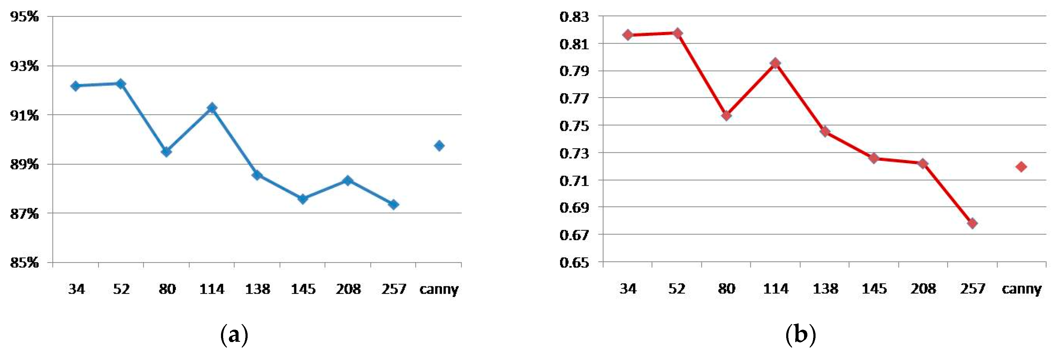
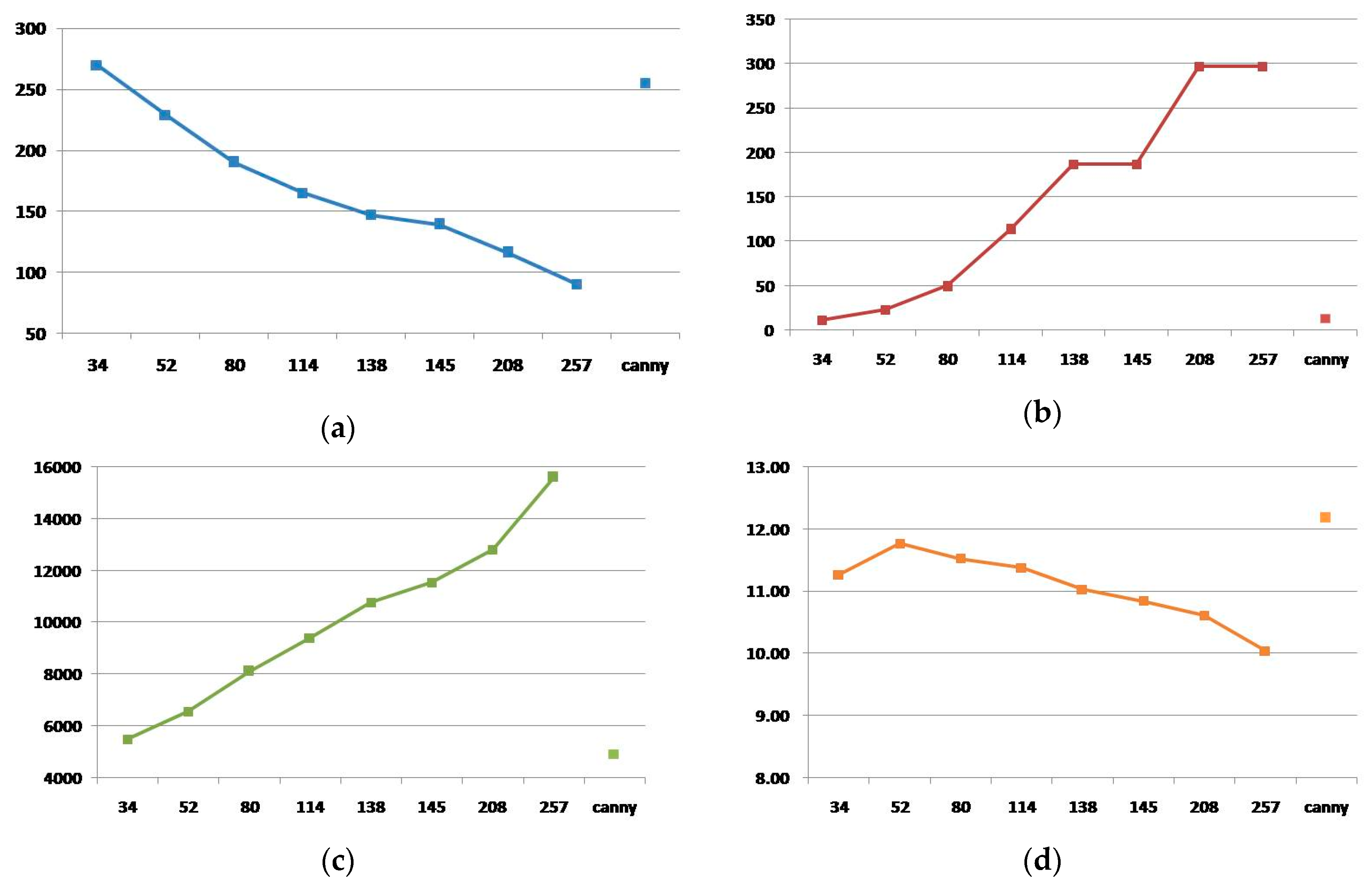
Figure 5 shows OA, kappa coefficients of agreement, PA, and UA assessed classifications generated by the two methods. As expected, a smaller segmentation scale (SC = 34, 52) yields higher accuracy, the highest overall accuracy of 92.26% with a Kappa of 0.82 was achieved. The results also demonstrate that the overall accuracy and kappa coefficient shows a declining trend with increasing scale (Figure 5a,b).
With an increase of segmentation scale, PA and UA of the three classes (corridor, yardang, and shadow) showed a different tendency. PA of corridor first decreased and then increased, reaching the lowest points (SC = 138, 145) with the values of 87.45%, 86.2%, while the variation trend of yardang’ PA was opposite to that of the corridor (Figure 5c). PA of yardang first increased and then decreased, reaching the highest points (SC = 138, 145) with the values of 98.26% and 98.17%. The variation trends of UA for the two classes (corridor and yardang) were opposite to that of PA. According to the confusion matrix (Appendix Table A1(1)–(8)), we can explain this strange phenomenon. With the increase of segmentation scale, the number of samples in diagonal (confusion matrix) for yardang first increased and then decreased, reaching the highest points (SC = 138, 145), while the number of samples in diagonal for corridor first decreased and then increased, reaching the lowest points (SC = 138, 145). With the increase of segmentation scale, corridors can easily be mistaken for yardangs as the dunes in the corridors have similar spectral and textural properties to yardangs. This phenomenon increases the number of samples in calculating UA and reduces the UA of yardangs.
Shadows generally have small areas. As the segmentation scale becomes larger, they are gradually divided into other categories, and the total number also decreases. So the PA of shadows shows an obvious decreasing trend, while the UA changes greatly (Figure 5c,d).
Different categories have different optimal segmentation scales, which depend on the size of the categories and the image characteristics. Accuracy is a good criterion to evaluate the optimal scale. In general, we will achieve a higher accuracy of the classification results when the segmentation scale is closer to the size of the optimal scale [60]. In our study, the three categories (corridor, yardang, and shadow) have different optimal scales according to the PA and values in the diagonal of the confusion matrix. Yardangs have the highest classification accuracy under medium segmentation scales (SC = 138, 145), while corridors should use smaller or larger segmentation scales to get a higher classification result. Since the size of shadows was obviously smaller than others, the smallest segmentation scale (SC = 34) was beneficial to the shadows.
Despite being unable to recognize shadows, the CED method achieved an overall accuracy of 89.23% with a kappa coefficient of 0.72 (Figure 5a,b; Appendix Table A1(9)), similar to that of a medium segmentation scale (SC = 138). For the CED method, the category of the corridor had higher PA and UA than the OBIA method (Figure 5c,d), as the manual interpretation could eliminate the phenomenon that dunes divided into yardangs. Though the category of yardang had a higher UA than the OBIA method, its PA was lower (the value 71.99% was similar to that of the largest segmentation scale (257)), indicating it is easy to miss yardangs using the CED method.
4.3. Geomorphological Characteristic Parameters
For the OBIA method, several manual editing steps are required to ensure the accuracy of the characteristic geomorphological parameters calculated on the basis of yardangs extracted: (1) We merged same-class adjacent objects; (2) re-labeled the shadows and corridors inside the yardangs into yardangs; (3) deleted the misclassified yardangs, but did not modify the yardang boundaries.
After extracting of yardangs from the very high-resolution image subset, with each being seen as a single object, we could calculate their geometric parameters (i.e., area, length, width, length/width ratio, and orientation). These parameters were calculated in units of pixels in the software, eCognition. We could get the characteristic geomorphological parameters of yardangs after converting the pixels into meters.
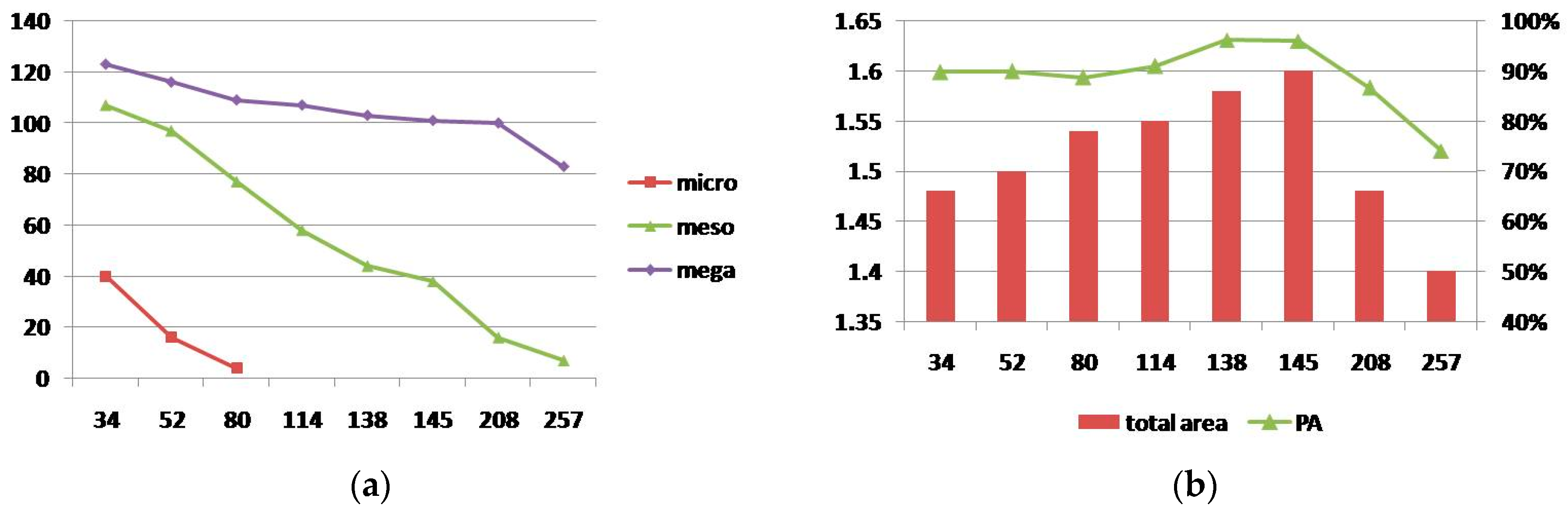
Figure 6 shows several morphological parameters of yardangs: total number, minimum area, mean area, and median direction. Larger segmentation scale generally leads to a smaller number of image objects with larger areas [48], so the total number of yardangs decreases while minimum area and mean area increase as the segmentation scale increases. CED method obtains satisfactory results, and the values of the three parameters (i.e., total number, minimum area, and mean area) are close to those of the smallest segmentation scale (SC = 34). The values of the median direction using the two methods were around 11°, which was similar to the calculated result by Dong et al. [20].
5. Discussion
5.1. The Effect of Segmentation Scales
Based on the size of the area, all of the yardangs could be divided into three sub-categories: micro-yardang (area ≤ 100 m2), meso-yardang (100m2 < area < 1000 m2), and mega-yardang (area ≥ 1000 m2). We wanted to analyze the relationship between yardang size and segmentation scale.
Figure 7a demonstrates the total number of the three types of yardangs under different segmentation scales. With an increase of segmentation scale, the number of the three types of yardangs decreased, micro-yardangs could only be identified using the smaller segmentation scale (SC = 34, 52, 80), only several meso-yardangs could be extracted under the highest segmentation scale (SC = 257).
Figure 7b shows that the PA of yardang extraction had a strong correlation with the total area. With an increase of segmentation scale, both of them demonstrated a tendency of initial increase (reaching the highest points when SC = 138, 145), followed by a decrease.
5.2. The Effect of Spatial Resolution
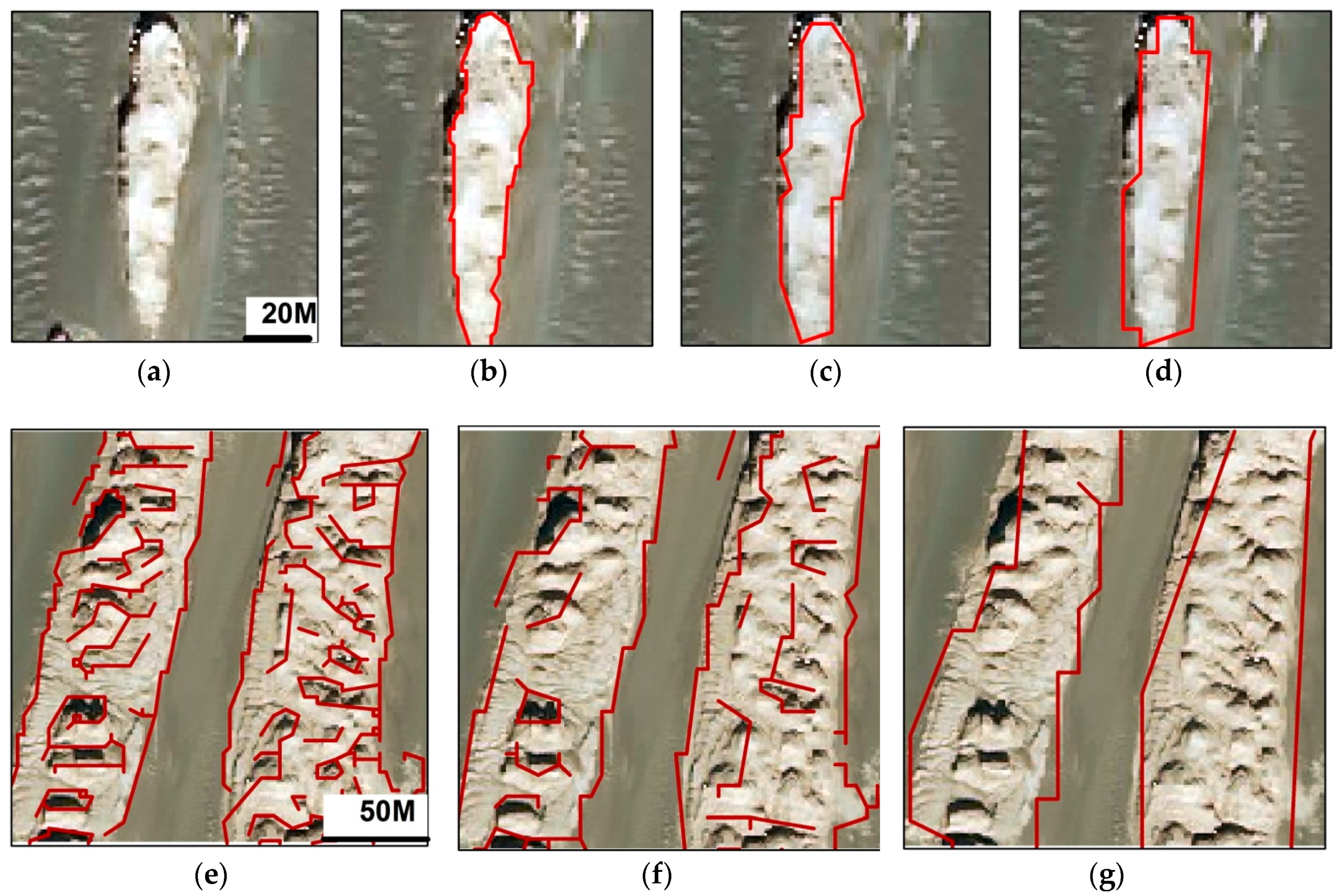
Using the resample method, the smoothing effects caused by the decrease (coarsening) of spatial resolution can reduce the spectral difference among yardangs, and it is easier to distinguish the boundaries of yardangs. With the decreasing of spatial resolution, the image information gradually decreases, and the edges of yardangs become clearer (Figure 8e–g). We analyzed the relationship between the total length of the extracted boundaries and the spatial resolution via Figure 9a, whereas a logarithmically decreasing trend is shown (R2 = 0.904).
The spatial resolution had a significant influence on the extraction of yardangs. For the same yardang, if the images with different resolutions could extract it in complete boundaries, then we could achieve more accuracy using the higher (finer) spatial resolution image (Figure 8a–d). Especially for mega yardangs, the boundaries became much clearer as the spatial resolution decreased (Figure 8e–g). Huang and Wu [60] concluded that spatial resolution has a linear relationship with the accuracy of the extracted objects. Ehsani and Quiel [33] showed that yardangs could be clearly recognized when their widths larger than the spatial resolution of DEM using a self organizing map method. In our study, we also analyzed the relationship between yardang size and spatial resolution. Figure 9b shows a linear relationship between the median widths of extracted yardangs and spatial resolutions (R2 = 0.95).
6. Conclusions
Two methods, which are efficient, low-cost, and semi-automatic, were proposed for extracting yardang parameters in this research. Using the OBIA classification method, we integrated geometric, spectral, and textural features to construct the feature space.Yardangs could be easily extracted from the very high spatial resolution image subset from Google Earth. The segmentation scale was the key factor in determining the size of yardangs. With an increase of segmentation scale, the number of the three types of yardangs decreased, micro-yardangs (area ≤ 100 m2) could only be identified using the smaller segmentation scale (SC = 34, 52, 80), while only several meso-yardangs (100 m2 < area < 1000 m2) could be extracted with the highest segmentation scale (SC = 257).
Using the CED method, resampling the image subset to a series of lower spatial resolution ones could effectively reduce noise. The total length of the yardang boundaries showed a logarithmically decreasing (R2 = 0.904) trend with decreasing spatial resolution. There is also a linear relationship between the median widths of yardangs and spatial resolutions (R2 = 0.95).
Confusion matrices were used to verify classification accuracies. The OBIA method achieved the highest overall accuracy of 92.26% with a Kappa of 0.82 at a smaller segmentation scale (SC = 52). Despite being unable to extract shadows, the CED method achieved an overall accuracy of 89.23% with a kappa coefficient of 0.72, similar to that of the OBIA method working at a medium segmentation scale (SC = 138).
Comparing the geomorphological characteristic parameters of yardangs using the two methods, the CED method gave rises to satisfactory results, and the values of the three parameters considered (i.e., total number, minimum area, and mean area) are close to those obtained using OBIA method atthe smallest segmentation scale (SC = 34). OBIA is more automatic, while CED is simpler but relies more on manual interpretation.
Author Contributions
Z.L. proposed and organized the research; W.Y. and W.Z. performed the experiments; J.Z. refined the experimental design. All authors contributed to writing the paper. All authors have read and agree to the published version of the manuscript.
Funding
This research was supported by the National Natural Science Foundation of China (No.41471375 and 41290252), and the Funding Program of International Exchanges and Cooperation for Graduate Students at CUG.
Acknowledgments
We thank Mahmoud Abbas for improving the English of an early version.
Conflicts of Interest
The authors declare no conflict of interest
Appendix A

Table A1.
Confusion matrix and accuracy assessment results using the two methods: (1)–(8) the OBIA method with different segmentation scales (SC) ((1) SC = 34,(2) SC = 52, (3) SC = 80, (4) SC = 114, (5) SC = 138, (6) SC = 145, (7) SC = 208, (8) SC = 257), and (9) Edge detection result using the CED method. Producer’s accuracy (PA), user’s accuracy (UA), and overall accuracy (OA).
| (1) | (2) | ||||||||
| corrider | yardang | shadow | sum | corrider | yardang | shadow | sum | ||
| corrider | 1512 | 51 | 2 | 1565 | corrider | 1514 | 52 | 5 | 1571 |
| yardang | 103 | 519 | 10 | 632 | yardang | 102 | 520 | 8 | 630 |
| shadow | 2 | 8 | 40 | 50 | shadow | 1 | 6 | 39 | 46 |
| sum | 1617 | 578 | 52 | sum | 1617 | 578 | 52 | ||
| PA | 93.50% | 89.80% | 76.92% | PA | 93.63% | 89.97% | 75.00% | ||
| UA | 96.61% | 82.12% | 80.00% | UA | 96.37% | 82.54% | 84.78% | ||
| OA | 92.17% | OA | 92.26% | ||||||
| kappa | 0.8161 | kappa | 0.8175 | ||||||
| (3) | (4) | ||||||||
| corrider | yardang | shadow | sum | corrider | yardang | shadow | sum | ||
| corrider | 1463 | 61 | 4 | 1528 | corrider | 1497 | 48 | 8 | 1553 |
| yardang | 153 | 513 | 13 | 679 | yardang | 119 | 526 | 16 | 661 |
| shadow | 1 | 4 | 35 | 40 | shadow | 1 | 4 | 28 | 33 |
| sum | 1617 | 578 | 52 | sum | 1617 | 578 | 52 | ||
| PA | 90.48% | 88.75% | 67.30% | PA | 92.58% | 91.00% | 53.85% | ||
| UA | 95.75% | 75.55% | 87.50% | UA | 96.40% | 79.58% | 84.85% | ||
| OA | 89.50% | OA | 91.28% | ||||||
| kappa | 0.7572 | kappa | 0.7955 | ||||||
| (5) | (6) | ||||||||
| corrider | yardang | shadow | sum | corrider | yardang | shadow | sum | ||
| corrider | 1414 | 18 | 7 | 1439 | corrider | 1394 | 19 | 7 | 1420 |
| yardang | 202 | 556 | 25 | 783 | yardang | 222 | 555 | 26 | 803 |
| shadow | 1 | 4 | 20 | 25 | shadow | 1 | 4 | 19 | 24 |
| sum | 1617 | 578 | 52 | sum | 1617 | 578 | 52 | ||
| PA | 87.44% | 96.20% | 38.46% | PA | 86.20% | 96.02% | 36.54% | ||
| UA | 98.26% | 71.00% | 80.00% | UA | 98.17% | 69.12% | 79.17% | ||
| OA | 88.56% | OA | 87.58% | ||||||
| kappa | 0.7454 | kappa | 0.726 | ||||||
| (7) | (8) | ||||||||
| corrider | yardang | shadow | sum | corrider | yardang | shadow | sum | ||
| corrider | 1478 | 76 | 19 | 1573 | corrider | 1529 | 150 | 25 | 1704 |
| yardang | 138 | 501 | 27 | 666 | yardang | 88 | 428 | 21 | 537 |
| shadow | 1 | 1 | 6 | 8 | shadow | 0 | 0 | 6 | 6 |
| sum | 1617 | 578 | 52 | sum | 1617 | 578 | 52 | ||
| PA | 91.40% | 86.68% | 11.54% | PA | 94.55% | 74.05% | 11.54% | ||
| UA | 93.96% | 75.23% | 75.00% | UA | 89.73% | 79.70% | 100.00% | ||
| OA | 88.34% | OA | 87.36% | ||||||
| kappa | 0.7223 | kappa | 0.6782 | ||||||
| (9) | |||||||||
| corrider | yardang | shadow | sum | ||||||
| corrider | 1562 | 135 | 44 | 1741 | |||||
| yardang | 55 | 443 | 8 | 506 | |||||
| shadow | 0 | 0 | 0 | 0 | |||||
| sum | 1617 | 578 | 52 | ||||||
| PA | 96.60% | 76.64% | 0.00% | ||||||
| UA | 89.72% | 87.55% | |||||||
| OA | 89.23% | ||||||||
| kappa | 0.7199 | ||||||||
References
- Fox, R.W.; McDonald, A.T. Introdution of Fluid Mechanics; Wiley: New York, NY, USA, 1973. [Google Scholar]
- Laity, J.E. Landforms of aeolian erosion. In Geonorphology of Desert Environments; Abrahams, A.D., Parsons, A.J., Eds.; Chapman and Hall: London, UK, 1994; Volume 674. [Google Scholar]
- Goudie, A.S. Wind Erosional Landforms: Yardangs and Pans; Wiley: Chichester, UK, 1999. [Google Scholar]
- Goudie, A.S. Mega-Yardangs: A Global Analysis. Geogr. Compass 2007, 1, 65–81. [Google Scholar] [CrossRef]
- Laity, J.E. Wind erosion in drylands. In Arid Zone Geomorphology: Process, Form and Change in Drylands, 3rd ed.; Thomas, D.S.G., Ed.; John Wiley & Sons, Ltd.: London, UK, 2011; pp. 539–567. [Google Scholar] [CrossRef]
- McCauley, J.F.; Grolier, M.J.; Breed, C.S. Yardangs. In Geomorphology in Arid Regions; Allen and Unwin: London, UK, 1977. [Google Scholar]
- Ward, A.W. Evolution of the yardangs at Rogers Lake, California. Geol. Soc. Am. Bull. 1984, 7, 829–837. [Google Scholar] [CrossRef]
- Laity, J.E. Landforms, Landscapes, and Processes of Aeolian Erosion. In Geomorphology of Desert Environments; Parsons, A.J., Ed.; Springer Science: New York, NY, USA, 2009; pp. 597–627. [Google Scholar] [CrossRef]
- Halimov, M.F.F. 8 yardangs types in central-Asia. Z. Geomorphol. 1989, 2, 205–217. [Google Scholar]
- Blackwelder, E. Yardangs. Bull. Geol. Soc. Am. 1934, 45, 159–165. [Google Scholar] [CrossRef]
- Cooke, R.U.; Warren, A.; Andrew, S.G. Desert Geomorphology; UCL Press: London, UK, 1993. [Google Scholar]
- Hedin, S. Central Asia and Tibet; Scribners: New York, NY, USA, 1903. [Google Scholar]
- Brookes, I.A. Aeolian erosional lineations in the Libyan Desert, Dakhla Region, Egypt. Geomorphology 2001, 39, 189–209. [Google Scholar] [CrossRef]
- Hu, C.; Chen, N.; Kapp, P.; Chen, J.; Xiao, A.; Zhao, Y. Yardang geometries in the Qaidam Basin and their controlling factors. Geomorphology 2017, 299, 142–151. [Google Scholar] [CrossRef]
- Gutiérrez-Elorza, M.; Desir, G.; Gutiérrez-Santolalla, F. Yardangs in the semiarid central sector of the Ebro Depression (NE Spain). Geomorphology 2002, 44, 155–170. [Google Scholar] [CrossRef]
- Li, J.; Dong, Z.; Qian, G.; Zhang, Z.; Luo, W.; Lu, J.; Wang, M. Yardangs in the Qaidam Basin, northwestern China: Distribution and morphology. Aeolian Res. 2016, 20, 89–99. [Google Scholar] [CrossRef]
- Clarke, M.L.; Wintle, A.G.; Lancaster, N. Infra-red stimulated luminescence dating of sands from the Cronese basins, Mojave desert. Geomorphology 1996, 1–3, 199–205. [Google Scholar] [CrossRef]
- Sebe, K.; Csillag, G.; Ruszkiczay-Rüdiger, Z.; Fodor, L.; Thamó-Bozsó, E.; Müller, P.; Braucher, R. Wind erosion under cold climate: A Pleistocene periglacial mega-yardang system in Central Europe (Western Pannonian Basin, Hungary). Geomorphology 2011, 134, 470–482. [Google Scholar] [CrossRef]
- Barchyn, T.E.; Hugenholtz, C.H. Yardang evolution from maturity to demise. Geophys. Res. Lett. 2015, 42, 5865–5871. [Google Scholar] [CrossRef]
- Dong, Z.; Lv, P.; Lu, J.; Qian, G.; Zhang, Z.; Luo, W. Geomorphology and origin of Yardangs in the Kumtagh Desert, Northwest China. Geomorphology 2012, 139–140, 145–154. [Google Scholar] [CrossRef]
- Mainguet, M. Un etonnantpaysage:lescanneluresgreseuse du Bembeche. Ann. Geogr. 1970, 79, 58–66. [Google Scholar] [CrossRef]
- Wang, Z.T.; Wang, H.T.; Niu, Q.H.; Dong, Z.B.; Wang, T. Abrasion of yardangs. Phys. Rev. E 2011, 84, 31304. [Google Scholar] [CrossRef] [PubMed]
- Wang, J.; Xiao, L.; Reiss, D.; Hiesinger, H.; Huang, J.; Xu, Y.; Zhao, J.; Xiao, Z.; Komatsu, G. Geological Features and Evolution of Yardangs in the Qaidam Basin, Tibetan Plateau (NW China): A Terrestrial Analogue for Mars. J. Geophys. Res. Planets 2018, 123, 2336–2364. [Google Scholar] [CrossRef]
- Greeley, R.; Bender, K.; Thomas, P.E. Wind-Related Features and Processes on Venus: Summary of Magellan Results. Icarus 1995, 2, 399–420. [Google Scholar] [CrossRef]
- Baker, V.R. The geomorphology of Mars. Prog. Phys. Geogr. 1981, 4, 473–513. [Google Scholar] [CrossRef]
- Xiao, L.; Wang, J.; Dang, Y.; Cheng, Z.; Huang, T.; Zhao, J.; Xu, Y.; Huang, J.; Xiao, Z.; Komatsu, G. A new terrestrial analogue site for Mars research: The Qaidam Basin, Tibetan Plateau (NW China). Earth Sci. Rev. 2017, 164, 84–101. [Google Scholar] [CrossRef]
- Paillou, P.; Seignovert, B.; Radebaugh, J.; Wall, S. Radar scattering of linear dunes and mega-yardangs: Application to Titan. Icarus 2016, 270, 211–221. [Google Scholar] [CrossRef] [Green Version]
- Zhao, Y.; Chen, N.; Chen, J.; Hu, C. Automatic extraction of yardangs using Landsat 8 and UAV images: A case study in the Qaidam Basin, China. Aeolian Res. 2018, 33, 53–61. [Google Scholar] [CrossRef]
- Niu, Q. Formation and Evolution Process of yardang Landforms—A Case Study in DunhuangYardang National Geo-Park; Cold and Arid Regions Environmental and Engineering Research Institute (CAREERI), Chinese Academy of Sciences (CAS): Lanzhou, China, 2011. [Google Scholar]
- Ritley, K. Yardangs and dome dunes northeast of tavanhar, gobi, mongolia. GSA Abstr. Programs 2004, 4, 33–36. [Google Scholar]
- Arlegui, L.E.; Soriano, M.A. Characterizing lineaments from satellite images and field studies in the central Ebro basin (NE Spain). Int. J. Remote Sens. 1998, 19, 3169–3185. [Google Scholar] [CrossRef]
- Qu, J.; Niu, Q.; Gao, D. Formation and Development Processes Pattern of DunhuangYardang Landforms; Geological Publishing House: Beijing, China, 2014. [Google Scholar]
- Ehsani, A.H.; Quiel, F. Application of Self Organizing Map and SRTM data to characterize yardangs in the Lut desert, Iran. Remote Sens. Environ. 2008, 112, 3284–3294. [Google Scholar] [CrossRef]
- Blaschke, T. Object based image analysis for remote sensing. ISPRSJ. Photogramm. 2010, 65, 2–16. [Google Scholar] [CrossRef] [Green Version]
- Georganos, S.; Grippa, T.; Vanhuysse, S.; Lennert, M.; Shimoni, M.; Kalogirou, S.; Wolff, E. Less is more: Optimizing classification performance through feature selection in a very-high-resolution remote sensing object-based urban application. Gisci. Remote Sens. 2018, 55, 221–242. [Google Scholar] [CrossRef]
- Cheng, J.; Bo, Y.; Zhu, Y.; Ji, X. A novel method for assessing the segmentation quality of high-spatial resolution remote-sensing images. Int. J. Remote Sens. 2014, 35, 3816–3839. [Google Scholar] [CrossRef]
- Liu, K.; Ding, H.; Tang, G.; Song, C.; Liu, Y.; Jiang, L.; Zhao, B.; Gao, Y.; Ma, R. Large-scale mapping of gully-affected areas: An approach integrating Google Earth images and terrain skeleton information. Geomorphology 2018, 314, 13–26. [Google Scholar] [CrossRef]
- Guo, Z.; Shao, X.; Xu, Y.; Miyazaki, H.; Ohira, W.; Shibasaki, R. Identification of Village Building via Google Earth Images and Supervised Machine Learning Methods. Remote Sens. Basel 2016, 8, 271. [Google Scholar] [CrossRef] [Green Version]
- Canny, J.F. A computation approach to edge detection. IEEE Trans. Pattern Anal. Mach. Intell. 1986, 8, 670–700. [Google Scholar] [CrossRef]
- Ding, L.; Goshtasby, A. On the Canny edge detector. Pattern Recognit. 2000, 34, 721–725. [Google Scholar] [CrossRef]
- Wang, Y.; Wu, F.; Zhang, X.; Zeng, P.; Ma, P.; Song, Y.; Chu, H. Formation and evolution of yardangs activated by Late Pleistocene tectonic movement in Dunhuang, Gansu Province of China. J. Earth Syst. Sci. 2016, 125, 1603–1614. [Google Scholar] [CrossRef] [Green Version]
- Yuan, X. The classification, Evaluation and the Sustainable Development of Geoheritages in Dunhuang; Yardang National Geopark: Gansu, China, 2014. [Google Scholar]
- Wu, F.; Ma, P.; Qiu, Z. Dunhuang Global Geopark of China; Geological Publishing House: Beijing, China, 2015. [Google Scholar]
- Benz, U.C.; Hofmann, P.; Willhauck, G.; Lingenfelder, I.; Heynen, M. Multi-resolution, object-oriented fuzzy analysis of remote sensing data for GIS-ready information. ISPRS J. Photogramm. 2004, 58, 239–258. [Google Scholar] [CrossRef]
- Myint, S.W.; Gober, P.; Brazel, A.; Grossman-Clarke, S.; Weng, Q. Per-pixel vs. object-based classification of urban land cover extraction using high spatial resolution imagery. Remote Sens. Environ. 2011, 115, 1145–1161. [Google Scholar] [CrossRef]
- Drǎguţ, L.; Tiede, D.; Levick, S.R. ESP: A tool to estimate scale parameter for multiresolution image segmentation of remotely sensed data. Int. J. Geogr. Inf. Sci. 2010, 24, 859–871. [Google Scholar] [CrossRef]
- Colkesen, I.; Kavzoglu, T. Selection of Optimal Object Features in Object-Based Image Analysis Using Filter-Based Algorithms. J. Indian Soc. Remote 2018, 46, 1233–1242. [Google Scholar] [CrossRef]
- Stumpf, A.; Kerle, N. Object-oriented mapping of landslides using Random Forests. Remote Sens. Environ. 2011, 2564–2577. [Google Scholar] [CrossRef]
- Zhang, C.; Li, G.; Cui, W. High-Resolution Remote Sensing Image Change Detection by Statistical-Object-Based Method. IEEE J. Stars 2018, 11, 2440–2447. [Google Scholar] [CrossRef]
- Haralick, R.M.; Shanmugam, K.; Dinstein, I. Textural Features for Image Classification. IEEE Trans. Syst. Man Cybern. 1973, 6, 610–621. [Google Scholar] [CrossRef] [Green Version]
- Huang, X.; Wen, D.; Li, J.; Qin, R. Multi-level monitoring of subtle urban changes for the megacities of China using high-resolution multi-view satellite imagery. Remote Sens. Environ. 2017, 196, 56–75. [Google Scholar] [CrossRef]
- Nussbaum, S.; Niemeyerb, I.; Canty, M.J. SEaTH—A new tool for automated feature extraction in the context of object-based image analysis for remote sensing. In Proceedings of the 1st International Conference on Object-based Image Analysis, Salzhourg, Austria; 2006. [Google Scholar]
- Zhang, Z.; Yu, T.; Meng, Q.; Hu, X.; Li, C. Image quality evalution of multi-scale resampling in geometric correction. J. Huazhong Norm. Univ. 2013, 47, 426–430. [Google Scholar]
- Lu, H.; Liu, Q.; Wang, Y.; Deng, X. A two-stage parametric subspace model for efficient contrast-preserving decolorization. Front. Inf. Technol. Electron. Eng. 2017, 18, 1874–1882. [Google Scholar] [CrossRef]
- Liu, Q.; Jiang, T. A study of translation arithmetic between color image and grey image. J. Wuhan Univ. Technol. 2003, 27, 344–346. [Google Scholar]
- Hao, M.; Shi, W.; Ye, Y.; Zhang, H.; Deng, K. A novel change detection approach for VHR remote sensing images by integrating multi-scale features. Int. J. Remote Sens. 2019, 40, 4910–4933. [Google Scholar] [CrossRef]
- Foody, G.M. Harshness in image classification accuracy assessment. Int. J. Remote Sens. 2008, 29, 3137–3158. [Google Scholar] [CrossRef] [Green Version]
- Kim, M.; Madden, M.; Warner, T.A. Forest Type Mapping using Object-specific Texture Measures from Multispectral Ikonos Imagery: Segmentation Quality and Image Classification Issues. Photogramm. Eng. Remote Sens. 2009, 75, 819–829. [Google Scholar] [CrossRef] [Green Version]
- Olofsson, P.; Foody, G.M.; Herold, M.; Stehman, S.V.; Woodcock, C.E.; Wulder, M.A. Good practices for estimating area and assessing accuracy of land change. Remote Sens. Environ. 2014, 148, 42–57. [Google Scholar] [CrossRef]
- Huang, H.; Wu, B. Analysis to the Relationship of Feature Size, Objects Scales, Image Resolution. Remote Sens. Technol. Appl. 2006, 21, 243–248. [Google Scholar]
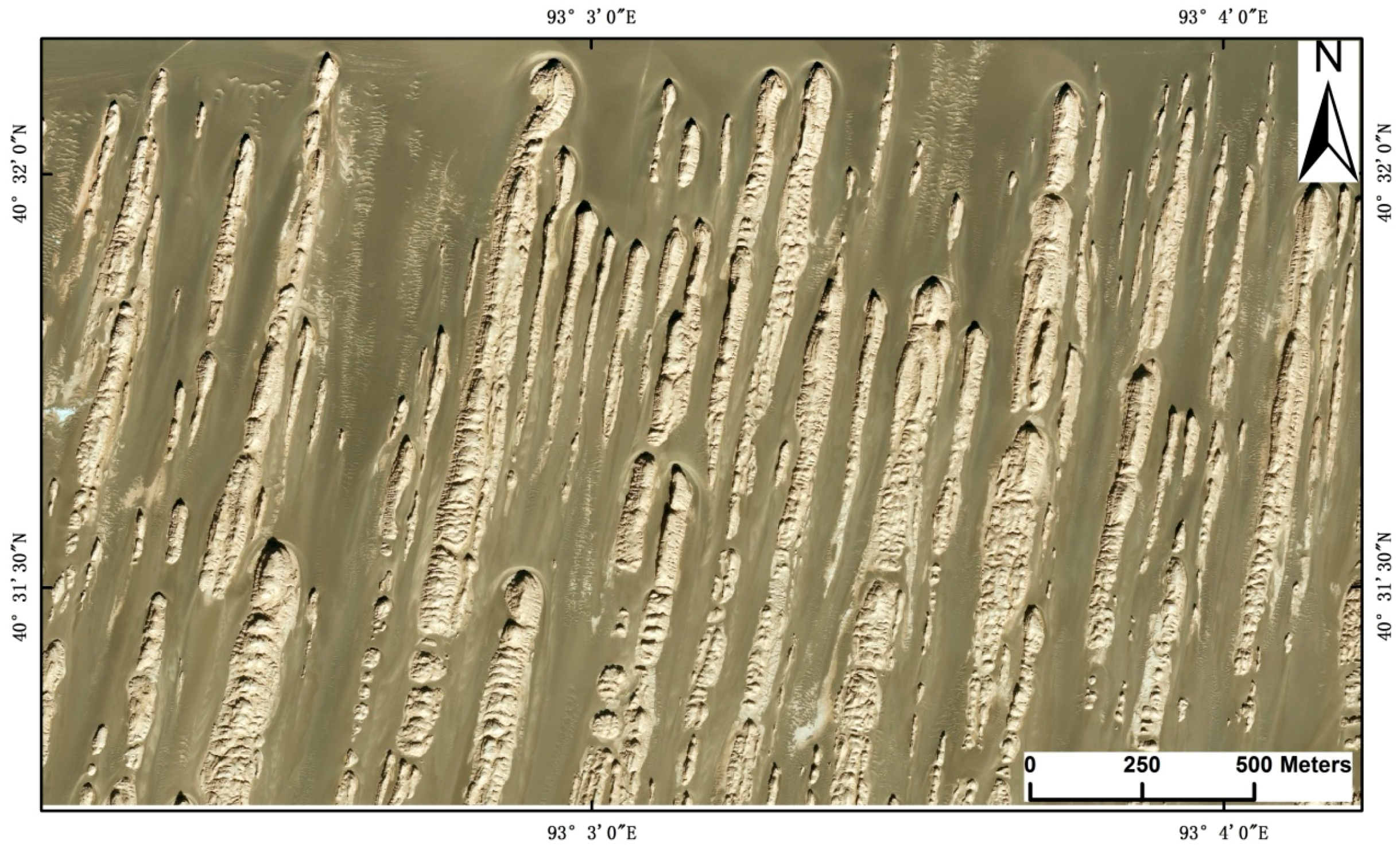
Figure 1.
The original very high-resolution image subset fromGoogle Earth (displayed in true color) of the study area.
Figure 1.
The original very high-resolution image subset fromGoogle Earth (displayed in true color) of the study area.

Figure 2.
Overview of the methods.

Figure 3.
Object levels with different segmentation scales (SC): (a) SC = 34, (b) SC = 80, (c) SC = 138, and (d) SC = 208.
Figure 3.
Object levels with different segmentation scales (SC): (a) SC = 34, (b) SC = 80, (c) SC = 138, and (d) SC = 208.


Figure 4.
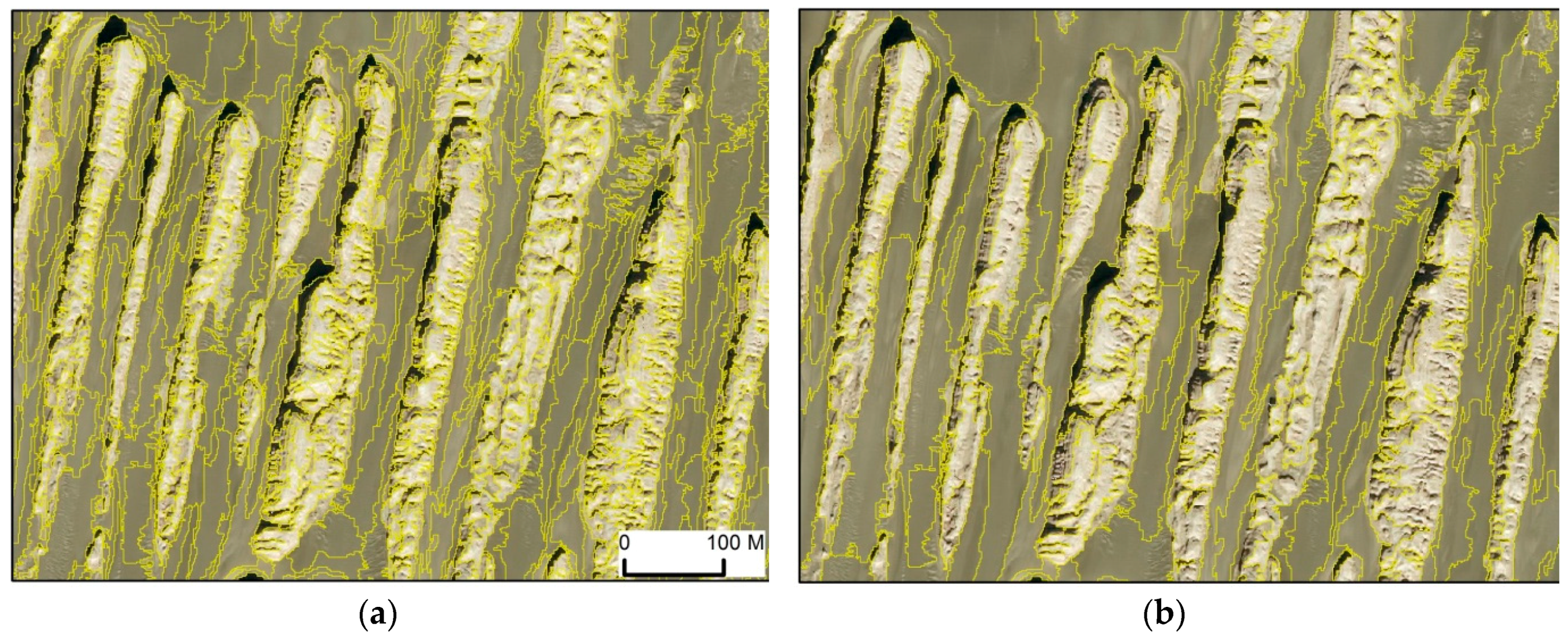
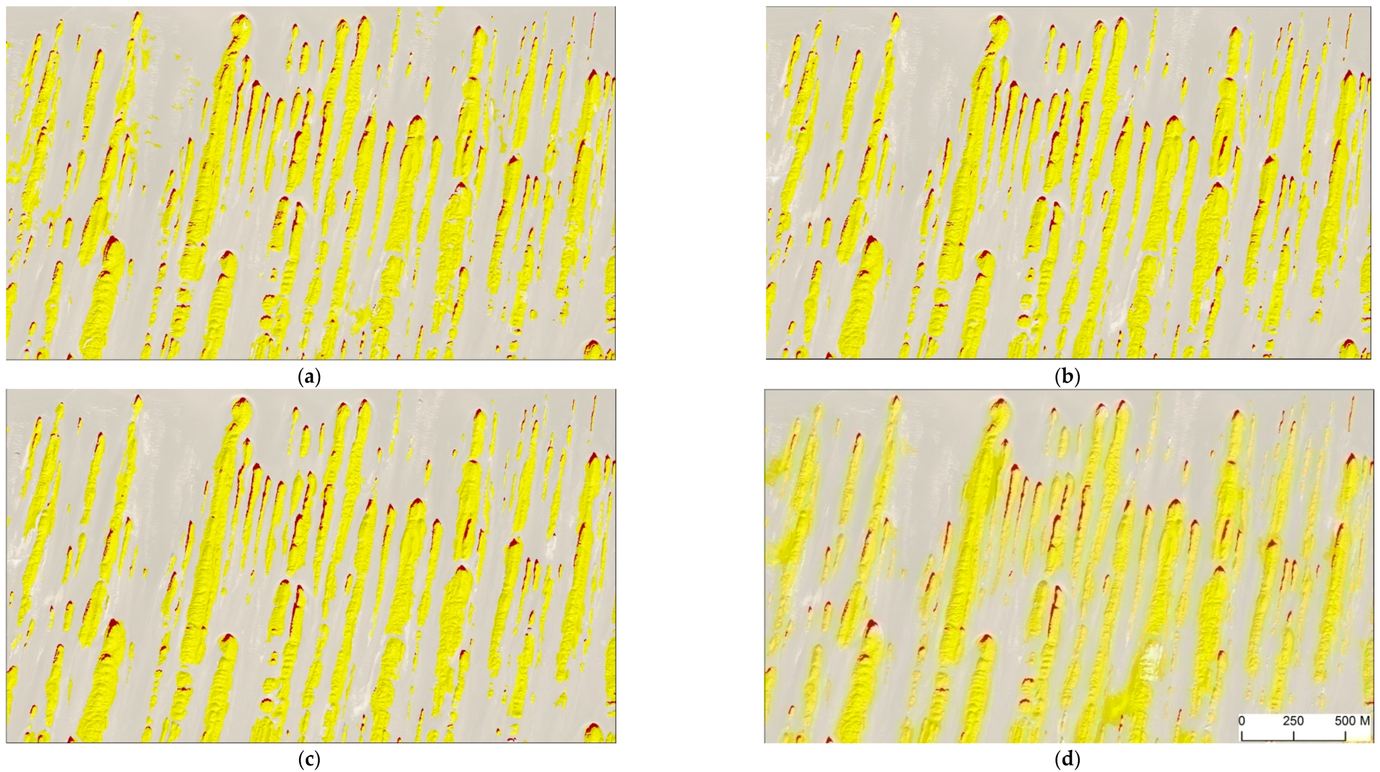
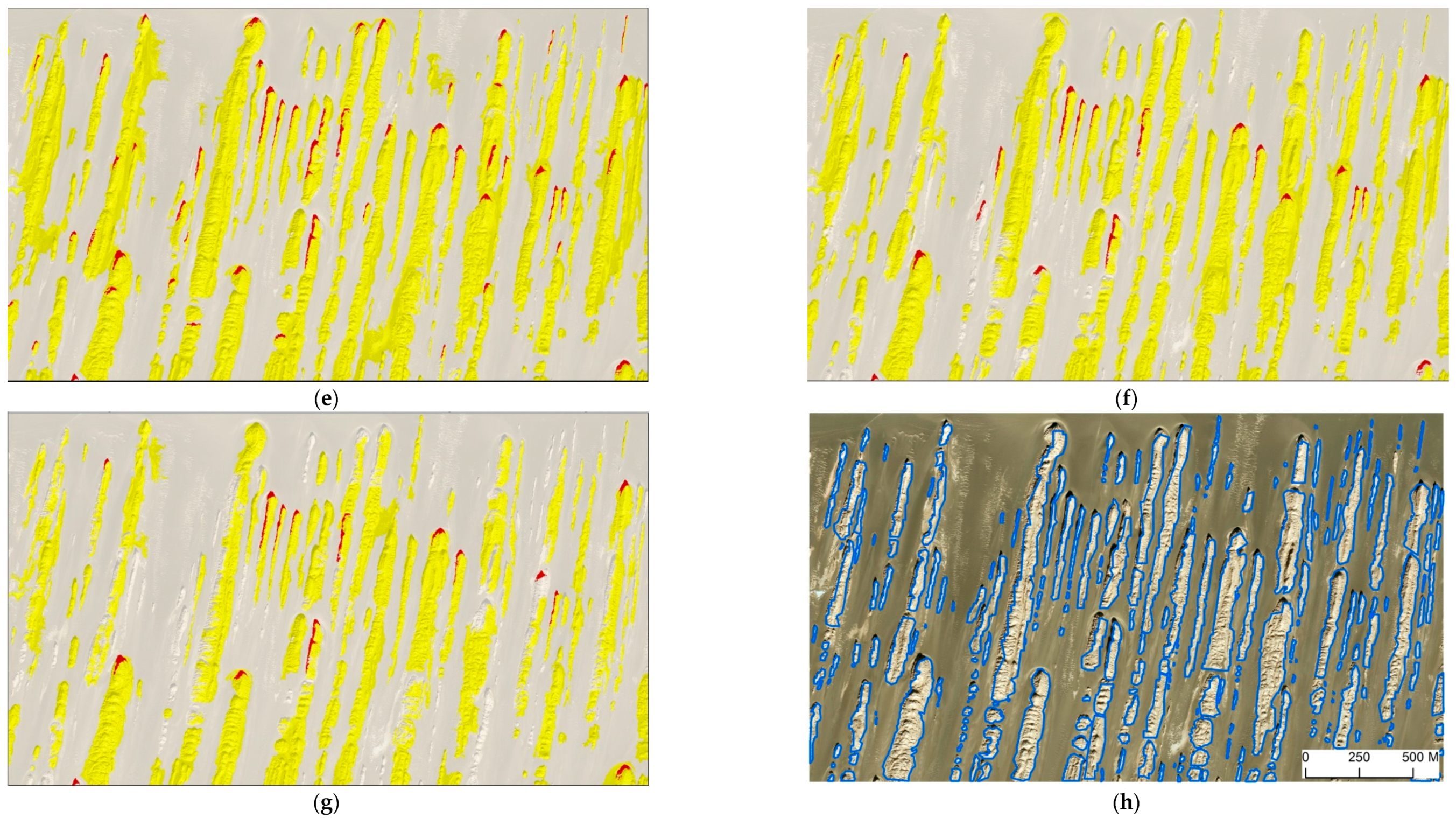
Classification results showing three classes, yardang (yellow), shadow (red), and corridor (light grey) using the two methods: (a)–(g) Object-based image analysis (OBIA) method with different segmentation scales (SC) ((a) SC = 34, (b) SC = 52, (c) SC = 80, (d) SC = 114, (e) SC = 145, (f) SC = 208, (g) SC = 257),and (h) Edge detection result using the Canny edge detection (CED) method.
Figure 4.
Classification results showing three classes, yardang (yellow), shadow (red), and corridor (light grey) using the two methods: (a)–(g) Object-based image analysis (OBIA) method with different segmentation scales (SC) ((a) SC = 34, (b) SC = 52, (c) SC = 80, (d) SC = 114, (e) SC = 145, (f) SC = 208, (g) SC = 257),and (h) Edge detection result using the Canny edge detection (CED) method.


Figure 5.
Accuracy curves with different segmentation scales and Canny edge detection: (a) OA, (b) Kappa, (c) PA, and (d) UA.
Figure 5.
Accuracy curves with different segmentation scales and Canny edge detection: (a) OA, (b) Kappa, (c) PA, and (d) UA.


Figure 6.
Statistical summary of a few yardang morphological parameters in the study area using the two methods: (a) the total number, (b) minimum area (m2), (c) mean area (m2), and (d) median direction (°).
Figure 6.
Statistical summary of a few yardang morphological parameters in the study area using the two methods: (a) the total number, (b) minimum area (m2), (c) mean area (m2), and (d) median direction (°).

Figure 7.
(a) The relationship between the total number of three types of yardangs under the different segmentation scales, (b) The relationship between the producer’s accuracy and the total area of yardang extraction.
Figure 7.
(a) The relationship between the total number of three types of yardangs under the different segmentation scales, (b) The relationship between the producer’s accuracy and the total area of yardang extraction.

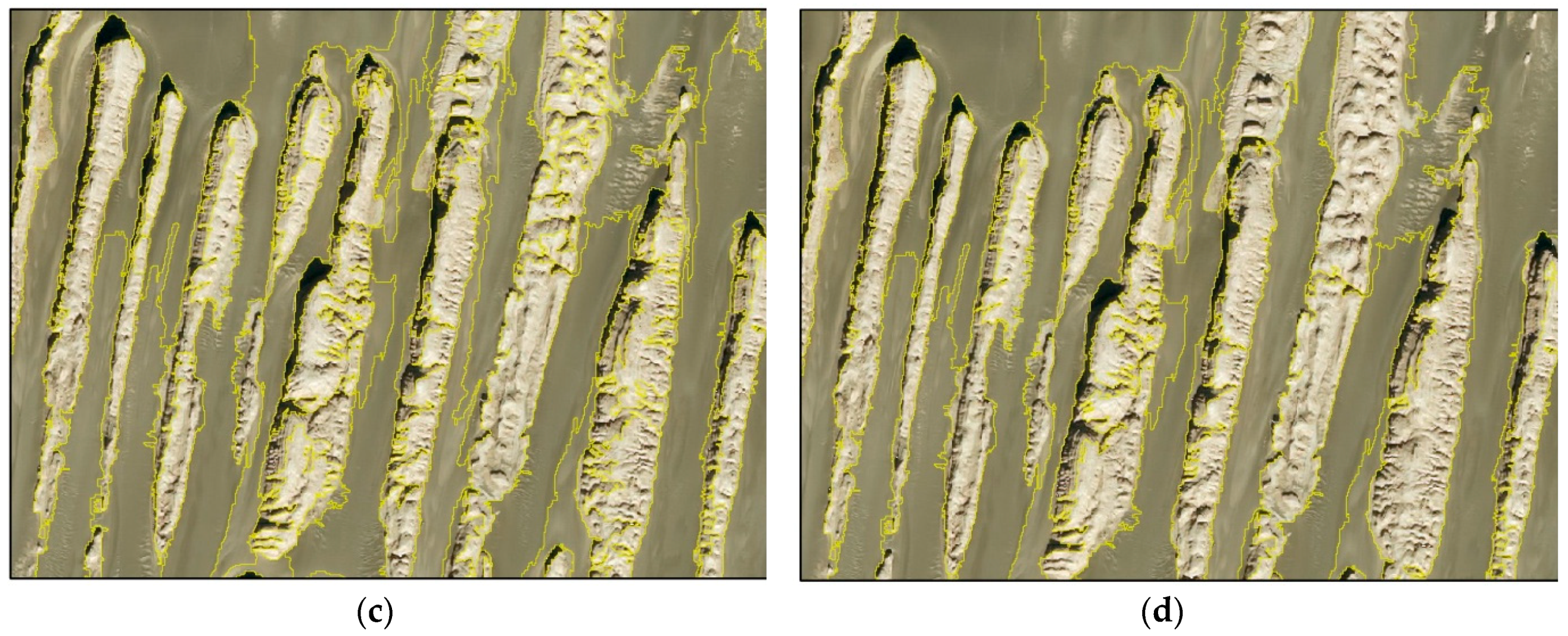
Figure 8.
The results of CED method with different spatial resolutions: (a) The original very high-resolution image subset in Google Earth, (b) 1.19 m, (c) 3 m, (d) 5 m, (e) 3 m, (f) 5 m, and (g) 10 m.
Figure 8.
The results of CED method with different spatial resolutions: (a) The original very high-resolution image subset in Google Earth, (b) 1.19 m, (c) 3 m, (d) 5 m, (e) 3 m, (f) 5 m, and (g) 10 m.

Figure 9.
(a) The relationship between the total length of the extracted boundaries and the spatial resolutions, (b) A linear relationship between the median widths of extracted yardangs using different spatial resolutions.
Figure 9.
(a) The relationship between the total length of the extracted boundaries and the spatial resolutions, (b) A linear relationship between the median widths of extracted yardangs using different spatial resolutions.

Table 1.
Optimization feature space under different segmentation scales (SC).
| SC = 34 | SC = 52 | SC = 80 | SC = 114 | SC = 138 | SC = 145 | SC = 208 | SC = 257 | |
|---|---|---|---|---|---|---|---|---|
| Spectral | SD layer (1,3) | SD layer (3) | SD layer (2,3) | SD layer (1,2) | SD layer (1,2, and 3) | SD layer (1,3) | SD layer (3) | SD layer (2,3) |
| mean layer (2) | mean layer (3) | mean layer (3) | mean layer (3) | mean layer (3) | mean layer (1,2, and 3) brightness | |||
| Texture | Hom (0°,45°) | Hom (0°,45°,all) | Hom (0°,45°,all) | Hom (0°,135°,all) | Hom (45°,135°) | Hom (45°,135°) | Hom (0°,45°) | Hom (0°) |
| mean (135°) | Con (0°) | Mean (0°,45°) | mean (0°) | mean (0°) | Con (0°) | |||
| Ent (all) | Ent (all) | Ent (all) | Ent (all) | Ent (0°) | Ent (45°) | Ent (0°) | ||
| Std (0°) | Con (45°) | |||||||
| Geometry | area | area | area | area | area | area | area | area |
| main direction | roundness | compactness | compactness | compactness | compactness | compactness | ||
| density | density | shape index | shape index density roundness | shape index |
© 2020 by the authors. Licensee MDPI, Basel, Switzerland. This article is an open access article distributed under the terms and conditions of the Creative Commons Attribution (CC BY) license (http://creativecommons.org/licenses/by/4.0/).
Share and Cite
MDPI and ACS Style
Yuan, W.; Zhang, W.; Lai, Z.; Zhang, J. Extraction of Yardang Characteristics Using Object-Based Image Analysis and Canny Edge Detection Methods. Remote Sens. 2020, 12, 726. https://0-doi-org.brum.beds.ac.uk/10.3390/rs12040726
AMA Style
Yuan W, Zhang W, Lai Z, Zhang J. Extraction of Yardang Characteristics Using Object-Based Image Analysis and Canny Edge Detection Methods. Remote Sensing. 2020; 12(4):726. https://0-doi-org.brum.beds.ac.uk/10.3390/rs12040726
Chicago/Turabian StyleYuan, Weitao, Wangle Zhang, Zhongping Lai, and Jingxiong Zhang. 2020. "Extraction of Yardang Characteristics Using Object-Based Image Analysis and Canny Edge Detection Methods" Remote Sensing 12, no. 4: 726. https://0-doi-org.brum.beds.ac.uk/10.3390/rs12040726
Note that from the first issue of 2016, this journal uses article numbers instead of page numbers. See further details here.