Article

Mitigation of Short-Term Temporal Variations of Receiver Code Bias to Achieve Increased Success Rate of Ambiguity Resolution in PPP

1
College of Geology Engineering and Geomatics, Chang’an University, Xi’an 710054, China
2
Department of Geomatics Engineering, University of Calgary, Calgary, AB T2N 1N4, Canada
3
National Key Laboratory of Geo-Information Engineering, Xi’an 710054, China
4
Xi’an Research Institute of Surveying and Mapping, Xi’an 710054, China
*
Author to whom correspondence should be addressed.
Submission received: 20 January 2020 / Revised: 25 February 2020 / Accepted: 26 February 2020 / Published: 2 March 2020

Abstract

:
Ambiguity resolution (AR) is critical for achieving a fast, high-precision solution in precise point positioning (PPP). In the standard uncombined PPP (S-UPPP) method, ionosphere-free code biases are superimposed by ambiguity and receiver clock offsets to be estimated. However, besides the time-constant part of the receiver code bias, the complex and time-varying term in receivers destroy the stability of ambiguities and degrade the performance of the UPPP AR. The variation of receiver code bias can be confirmed by the analysis in terms of ionospheric observables, code multipath (MP) of the Melbourne–Wübbena (MW) combination and the ionosphere-free combination. Therefore, the effect of receiver code biases should be rigorously mitigated. We introduce a modified UPPP (M-UPPP) method to reduce the effects of receiver code biases in ambiguities and to decouple the correlation between receiver clock parameters, code biases, and ambiguities parameters. An extra receiver code bias is set to isolate the code biases from ambiguities. The more stable ambiguities without code biases are expected to achieve a higher success rate of ambiguity resolution and a shortened convergence time. The variations of the receiver code biases, which are the unmodeled errors in measurement residuals of the S-UPPP method, can be estimated in the M-UPPP method. The maximum variation of the code biases is up to 16 ns within two-hour data. In the M-UPPP method, the averaged epoch residuals for code and phase measurements recover their zero-mean features. For the ambiguity-fixed solutions in the M-UPPP method, the convergence times are 14 and 43 min with 17.7% and 69.2% improvements compared to that in the S-UPPP method which are 17 and 90 min under the 68% and 95% confidence levels.

1. Introduction

A major problem in facilitating precise point positioning (PPP) ambiguity resolution is that the undifferenced ambiguities are not integer values, due to the existence of the code and phase delay biases [1,2,3,4,5,6]. Fractional-cycle biases (FCB) in global navigation satellite system (GNSS) phase measurements must therefore be corrected or removed in order to recover the integer property of ambiguities [2,7,8,9,10,11,12]. In fact, these biases are hardware-dependent and exist in all receivers and satellites [13]. Furthermore, it is not possible to uniquely determine the integer values of ambiguities due to their linear correlation with the code and phase hardware-induced biases [14,15].
Code and phase biases are difficult to estimate with the undifferenced model, as they are highly correlated with clock offsets [16,17,18,19,20,21]. The International GNSS Service (IGS) has routinely generated differential code bias (DCB) products, in some case to compensate the code biases for aligning the observables and clocks or for using external ionospheric information [22]. The average monthly stability by daily DCB indices that are calculated as the standard deviation (STD) of the daily satellite DCBs are 0.11, 0.18, 0.17, and 0.14 ns for GPS, GLONASS, BDS, and Galileo over a two-year span from 2013 to 2014, respectively [23]. In fact, GNSS satellite DCBs remain fairly stable over considerable periods of time for different GNSS constellations [24,25,26,27]. Satellite DCBs can be treated as time-constant terms over a one-day period in the positioning process [28]. According to the Ionospheric Associate Analysis Centers (IAACs) and fast precise point positioning (Fast-PPP) models, the daily accuracy of satellite DCBs is about 0.12–0.20 and 0.07 ns, respectively [28]. The receiver DCBs, however, have shown significant inter-day variability [28,29,30,31,32]. For instance, fluctuations greater than 9 ns were found between two consecutive hours, and this correlated with the receiver hardware updates and receiver temperature variations [24,30]. The authors of [29] demonstrated the DCB variation in a receiver might be up to 6.5 ns over the course of one day. The natures of the temporal scale variation of receiver code biases have already been analyzed by many previous studies, and many different approaches have been adopted to deal with them in ionosphere modeling [30,31,32].
In the standard uncombined PPP (S-UPPP) method that was proposed in [18,33], by using the IGS satellite precise orbits and clock offsets products, the satellite and receiver code biases are treated as constants that are coupled with clock offsets and ambiguities. With the IGS precise satellite clock and DCBs products, under the assumption that the satellite DCB is quite stable, only the receiver code bias should be rigorously analyzed. The receiver ionosphere-free combined code bias is lumped with the receiver clock offset parameters and ambiguities, while the ambiguities are estimated as constants and only assimilate the time-constant part of the ionosphere-free combined code bias. The time-varying code biases must be accommodated by the least-squares residuals or ionosphere parameters in the uncombined PPP (UPPP) method. However, the large fluctuation of the code biases over a short-time period destroys the time-constant nature of the ambiguities and achieves a suboptimum solution. To mitigate the receiver code biases, the authors of [2] estimated the single-differenced (between satellites) fractional-cycle biases from a network solution to recover the integer nature of the ambiguities at a single station. This method eliminated the effect of the receiver code biases in a network solution. However, the accuracy of ambiguity estimates of a single station is not adequate enough to obtain a fixed ambiguity resolution due to the effect of large code bias variations [5]. In the S-UPPP method with raw measurements, by using IGS satellite clock products and satellite code biases called (which are known as the satellite DCB) without satellite phase biases corrections, satellite phase biases and the ionosphere-free code biases are lumped into user phase ambiguities [11,15,16]. Though the single difference observables between satellites have been discussed in previous research, undifferenced equations are used in practical processes. Consequently, the receiver ionosphere-free code bias is lumped in with the receiver clock error parameter for code measurements. In carrier phase measurements, the same receiver clock errors are estimated. Hence, user ambiguities passively reduce the content of receiver ionosphere-free code bias to hold the carrier phase equation [33]. With the elevation-dependent weighting of carrier phase measurements, the large code bias variations affect ambiguity estimation, especially during the initial period of convergence. This negatively impacts the estimation of float ambiguities to create different ambiguities for fixing integer ambiguities. The integer recovery clock (IRC) method was proposed to estimate satellite phase clock offset products with fixed integer ambiguities. With those satellite clock offsets, which are known as integer phase clock offsets and include satellite fractional-cycle biases, code biases have been separated from the ambiguities, and the integer nature of ambiguities has been directly recovered. Meanwhile, the independent receiver phase and code clock offsets can be estimated [5]. The authors of [6] improved the IRC method, which is known as the decoupled clock model (DC) method, to estimate satellite code and phase clock offsets with integer ambiguity. Compared to the FCB method, the IRC and DC models regard the receiver code, the satellite code, and the phase biases as non-constant clock-like terms [16,34]. However, the estimation of the integer phase clock offset or decoupled satellite clock offset increases the computational burden, and these clock offset products are also not compatible with the IGS official clock offset products. These two methods are not flexible for common users. Though the satellite code bias has shown a high stability over a period of one day, the stability of receiver code bias is heavily dependent on receiver temperature variation and firmware quality [31,35,36]. Hence, only specific receivers whose code biases are stable over one day by preliminary analysis are used to estimate the satellite ephemeris and clock offsets or FCBs in a network solution [10]. However, a wide variety of receiver types are adopted for users, and their code biases properties are not explicit known, especially in real-time applications.
To confirm the variation of the receiver code bias, the ionospheric observables obtained from carrier-to-code leveling (CCL) and UPPP were analyzed to confirm the stability of the between-receiver differential code bias (BR-DCB). To exclude the effects of the code multipath (MP) and ionospheric delays, the Melbourne–Wübbena (MW) and ionosphere-free combinations can be used to present the code multipath [37]. To eliminate the adverse impact of the variability of receiver code biases on ambiguity estimations in PPP, a modified uncombined PPP (M-UPPP) model is introduced to separate the receiver code biases from the ambiguity parameters. By using a similar treatment as in the IRC and DC models for receiver clock offsets, the independent clock offset terms are introduced in the model for the code and phase measurements, respectively.
The following sections start with detailed formulations of the CCL method with the MW combination, the ionosphere-free code multipath, and the UPPP model. Then, the introduced M-UPPP method is presented with the key point of ambiguity datum. The data and experimental setup are introduced in the next section. In the subsequent section, the analysis of receiver code bias variations and positioning performance of the M-UPPP method are presented. The statistic results of the convergence time and the ambiguity fixing success rate when using the M-UPPP method applied to over 220 stations are also shown in this section. Finally, a discussion of the results, conclusions, and perspectives are provided.

2. Methods

Firstly, the linearized code and phase basic observation equations are derived. Then, the carrier-to-code leveling method and the uncombined PPP method are introduced to extract ionospheric observations for detecting receiver code bias variations. The geometry-free and ionosphere-free combinations are also adopted to evaluate the multipath measurements for detecting the receiver code bias variations. Additionally, through an analysis of related formulas, the M-UPPP method is be introduced to improve the performance of positioning and ambiguity resolution. In the following, the ambiguity datum of the M-UPPP method is explained.

2.1. Basic Code and Phase Observation Equations

The dual-frequency basic code and phase observation equations are described as:
{ P r , f s = ρ + c ( d t r d t s ) + T + γ f I r , 1 s                 + ( d r , f + δ d r , f ) ( d f s + δ d f s ) + m P , f s + ε P , f Φ r , f s = ρ + c ( d t r d t s ) + T γ f I r , 1 s + λ f N r , f s + ( b r , f + δ b r , f ) ( b f s + δ b r , f ) + m Φ , f s + ε Φ , f
where P r , f s is the code measurement at frequency f ( f = 1 , 2 ) for satellite s (m); Φ r , f s is the carrier phase measurement at frequency f ( f = 1 , 2 ) (m), ρ is the geometric range between receiver r and satellite s ; c is the speed of light in vacuum; d t r is the receiver clock offset; d t s is the satellite clock offset; T is the slant troposphere delay; I 1 is the ionospheric delay along the line-of-sight of receiver and satellite at the first frequency and γ f = λ f 2 / λ 1 2 ; λ f is the wavelength at frequency f (m); N r , f s is the phase ambiguity at frequency f (cycle); d r , f and d f s are the constant code biases at frequency f for the receiver and the satellite in meters, respectively; δ d r , f and δ d f s are corresponding time-varying terms; b r , f and b f s are the phase biases at frequency f for receiver and satellite in meters, respectively; δ b r , f and δ b f s are corresponding time-varying terms; m P , f s and m Φ , f s are the code and the phase multipath, respectively; and ε P , f and ε Φ , f are the noises of the code and carrier phase measurements.

2.2. Detection of Receiver Code Bias

2.2.1. Carrier-to-Code Leveling (CCL) Method

To analyze the receiver code biases, differences between two receivers’ ionospheric observables estimated from the CCL method are useful for detecting bias variations. The CCL method is commonly adopted to directly extract the ionospheric observables with code and phase geometry-free (GF) combinations. This geometry-free combination is illustrated in the following [38]:
P r , 4 s = P r , 2 s P r , 1 s = ( γ 2 1 ) I r , 1 s + ( D C B s + δ D C B s ) ( D C B r + δ D C B r ) + m r , P 4 s + ε P 4 Φ r , 4 s = Φ r , 1 s Φ r , 2 s = ( γ 2 1 ) I r , 1 s + ( λ 2 N r , 1 s λ 1 N r , 2 s ) + ( D P B r + δ D P B r ) ( D P B s + δ D P B s ) + m r , Φ 4 s + ε Φ 4
where P r , 4 s and Φ r , 4 s are the GF combinations for code and phase measurements, respectively; D C B r = d r , 1 d r , 2 and D C B s = d 1 s d 2 s are the constant differential code biases (DCB) for the receiver and the satellite, respectively, δ D C B r = δ d r , 1 δ d r , 2 and δ D C B s = δ d 1 s δ d 2 s are the time-varying terms; D P B r = b r , 1 b r , 2 and D P B s = b 1 s b 2 s are the differential phase biases (DPB) for the receiver and the satellite, respectively, with the time-varying terms δ D P B r = δ b r , 1 δ b r , 2 and δ D P B s = δ b 1 s δ b 2 s . Hence, we formulate the Melbourne–Wübbena (MW) combination in detail to analyze the GF ambiguity as:
λ 4 N r , 4 s = Φ r , 4 s P r , 4 s = λ 1 N r , 1 s λ 2 N r , 2 s + ( D P B r + δ D P B r ) ( D P B s + δ D P B s ) + ( D C B r + δ D C B r ) ( D C B s + δ D C B s ) + ( m r , Φ 4 s m r , P 4 s ) + ( ε r , Φ 4 ε r , P 4 )
In the CCL method, the phase measurement can be corrected by the averaged GF ambiguities. The carrier-phase smoothed code measurement can be formulated as:
L r , c c l s = Φ r , 4 s Φ r , 4 s P r , 4 s a r c = ( γ 2 1 ) I r , 1 s + D c c l s D r , c c l + d l e v e l i n g + m r , c c l s + ε c c l
where d l e v e l i n g denotes the leveling errors, which means the averaged ambiguity bias that is caused by the code biases and the multipath. For one satellite, it is a constant value over a continuous observation arc. We also define the receiver and satellite biases, the multipath and measurement noise terms in detail. The receiver bias is denoted as:
D r , c c l = ( D P B r D P B r ) + ( δ D P B r δ D P B r ) + ( D C B r + δ D C B r )
Similarly, we denote the satellite biases as:
D c c l s = ( D P B s D P B s ) + ( δ D P B s δ D P B s ) + ( D C B s + δ D C B s )
Additionally, we denote the multipath and the measurements noises as:
{ m r , c c l s = m r , Φ 4 s m r , Φ 4 s + m r , P 4 s ε c c l = ε Φ 4 ε Φ 4 + ε P 4
Hence, when considering all bias terms in the formulation, the ionospheric observables obtained in the CCL method include the slant total electron content (STEC), the receiver and satellite biases, leveling errors, and the multipath and measurements noises. The phase-multipath and measurement noise can be neglected because of the high precision of the phase measurements. Here, we also excepted the carrier phase multipath and measurement noise in our following analysis. Code multipath was eliminated due to averaging processing of GF combined ambiguities. As such, Equation (4) can be represented as:
L r , c c l s = ( γ 2 1 ) I r , 1 s + D c c l s D r , c c l + d l e v e l i n g
Consider that two receivers (marked A and B) create a short or a zero baseline. A single difference that cancels the STEC and satellite bias is built to evaluate the variation of the receiver bias, which mainly covers the receiver code bias, over a continuous observation arc. Hence, this single difference, called the between receiver differential code bias (BR-DCB), is presented as:
Δ L A B , c c l s = L A , c c l s L B , c c l s = ( D A , c c l D B , c c l ) + d A , l e v e l i n g d B , l e v e l i n g
From Equation (5), we know that if the time-varying part of differential phase bias is insignificant, the BR-DCB in Equation (9) for one satellite over a continuous arc is constant. All observations of satellites are useful to detect the behavior of the receiver code biases [26,29].

2.2.2. Ionosphere-Free Code and Phase Combinations

In ionosphere-free code and phase combinations, the first-order ionospheric delays are removed. We define the following terms as:
{ α 12 = γ 2 γ 2 1 β 12 = 1 1 γ 2 d r , i f = α 12 d r , 1 + β 12 d r , 2 δ d r , i f = α 12 δ d r , 1 + β 12 δ d r , 2 d i f s = α 12 d 1 s + β 12 d 2 s δ d i f s = α 12 δ d 1 s + β 12 δ d 2 s b r , i f = α 12 b r , 1 + β 12 b r , 2 δ b r , i f = α 12 δ b r , 1 + β 12 δ b r , 2 b i f s = α 12 b 1 s + β 12 b 2 s δ b i f s = α 12 δ b 1 s + β 12 δ b 2 s
where α 12 and β 12 are ionosphere-free combination coefficients on each frequency that are used to formulate the ionosphere-free code and phase bias, respectively, for satellite, receiver constant, and time-varying terms. We used the ionosphere-free phase combination minus the code combination to analyze the variation of ionosphere-free code biases and the ionosphere-free code multipath. Here, we also neglected the carrier phase multipath and measurements noise.
L P c i f = Φ r , i f s P r , i f s = λ i f N i f + ( b r , i f + δ b r , i f ) ( b i f s + δ b i f s ) ( d r , i f + δ d r , i f d i f s δ d i f s ) + m r , P i f s
We used this difference to analyze the ionosphere-free code bias variations and be free of ionospheric delays effects.

2.2.3. Uncombined PPP Method

The unknown parameters, receiver and satellite clock offsets, code and phase delay biases, and ambiguities in Equation (1) are correlated. Hence, these parameters cannot be simultaneously estimated in a least-squares adjustment. In practice, only the coordinates, the tropospheric zenith wet delay, receiver clock error, ionospheric delays and ambiguity parameters are estimated in the UPPP method. In practice, the satellite clock offsets are corrected by IGS precise clock products. The satellite clock parameters are still exhibited in equations for the convenient analysis of other parameters. The code biases are assimilated into the clock offsets. Due to just one clock offset parameter for code and phase measurements, the ambiguities, code and phase biases are combined as one parameter. Considering the time-varying phase bias, the estimated clock parameters are defined as [16,39]
{ d t ˜ r = d t r + ( d r , i f + δ b r , i f ) / c d t ˜ s = d t s + ( d i f s + δ b i f s ) / c
where d t ˜ r and d t ˜ s are reparametrized clock offsets for the receiver and the satellite, respectively. While ionospheric delays are eliminated by the ionospheric-free combination, these delays have to be estimated in case of raw observations in the UPPP method without the extra ionospheric information constraints [40]. In the UPPP method, the ionospheric delays and ambiguities are reparametrized as
{ I ˜ r , 1 s = I r , 1 s 1 γ 2 1 ( D C B r D C B s ) + 1 γ 2 1 ( δ D P B r δ D P B s ) N ˜ r , f s = N r , f s + ( b r , f b f s ) / λ f ( d r , i f d i f s ) / λ f γ f γ 2 1 ( D C B r D C B s ) / λ f
where I ˜ r , 1 s is the reparametrized ionospheric delay parameter and N ˜ r , f s is the reparametrized ambiguity parameter. Hence, the S-UPPP model with code and phase measurements can be expressed as [16,39]:
{ P r , f s = ρ + c ( d t ˜ r d t ˜ s ) + T + γ f I ˜ r , 1 s                 + e P , f Φ r , f s = ρ + c ( d t ˜ r d t ˜ s ) + T γ f I ˜ r , 1 s + λ f N ˜ r , f d + ε Φ , f e P , f = δ d r , f δ d f s + δ b i f s δ b r , i f γ f γ 2 1 ( δ D P B r δ D P B s ) + ε P , f
where e P , f denotes the code measurement residuals. In Equations (13) and (14), the ionospheric delays and ambiguity parameters are estimated together with the receiver constant code bias. This assumption is based on the fact that the time-varying code bias should be assimilated into the code residuals due to the far-weak weights posed on code measurements. Hence, the time-varying code bias on each frequency is completely assimilated into the code residuals e P , f . However, the code biases d r , f , δ d r , f , and ambiguity N r , f s are strongly correlated. The effects on ambiguity estimation of code bias variation should not be neglected. With extreme variations of code bias in a short time, the model in Equation (14) would not achieve an optimal solution. In fact, large variation of code bias in short time degrade the estimation accuracy of ionospheric delays and ambiguities. The unmodeled variations of the receiver code bias in this S-UPPP must be rigorously taken into consideration. Hence, we introduce the M-UPPP model according to the PPP-RTK method [11,12] and the DC model [6].

2.3. Modified Uncombined PPP Model with Estimation of Receiver Code Bias

2.3.1. Modified Uncombined PPP Model

In the S-UPPP model, we assume that the constant code bias is assimilated into the clock offsets and ambiguities, while the time-varying code bias is assimilated into code residuals [16]. To consider the effects of code bias on estimation of clock offsets and ambiguities, the M-UPPP method is introduced to decrease the correlation between code bias and ambiguity. In fact, the hardware biases for satellites are stable enough to meet the previous assumption, while the variability of the receiver code biases is relatively conspicuous. Consequentially, the time-constant character of ambiguities are affected by the variational receiver code biases. Therefore, it is important to separate most code bias components from ambiguities in carrier phase observation. Similar as in the DC method for decoupling the code and phase clock parameters, we isolated receiver code bias from the phase ambiguities to improve the performance of PPP or ambiguity resolution. Here, we define the d r , P as the difference of the code and phase receiver clocks, which denotes the relative receiver code bias. Hence, Equation (14) can be expressed as:
{ P r , f s = ρ + c ( d t r , Φ + d r , P d t ˜ s ) + T + γ f I ˜ r , 1 s                   + e P , f Φ r , f s = ρ + c ( d t r , Φ           d t ˜ s ) + T γ f I ˜ r , 1 s + λ f N ˜ r , f s + ε Φ , f
where the ambiguity term N ˜ r , f s is denoted as:
{ N ˜ r , f s = N r , f s + ( b r , f b f s ) / λ f + d i f s / λ f γ f γ 2 1 ( D C B r D C B s ) / λ f e P , f = γ f γ 2 1 δ D C B r δ d f s + δ b i f s δ b r , i f γ f γ 2 1 ( δ D P B r δ D P B s ) + e P , f
where e P , f is the new code residuals in the M-UPPP method. Compared to ambiguity parameter in Equation (13), the ambiguity in Equation (16) is free of the effects of ionosphere-free receiver combined code bias. As already proposed [11,18], if ionospheric delay corrections are available, the receiver DCB can be estimated as an unknown parameter in the UPPP method. Hence, the receiver code bias, D C B r is separated from ambiguities parameters. With ionospheric constrained information, ambiguities are rigorously treated as constant and are free of all receiver code bias content [11,12].

2.3.2. Ambiguity Datum Fixing and Receiver Code Bias Content

Though the code biases in the M-UPPP method have been separated from the ambiguities, the lack of datum for receiver phase clock offset and ambiguities should be taken into consideration. If the ambiguities have been fixed to a determined value, the phase clock offset parameter can be fixed to a specific value without the help of code measurement. With this specific datum of ambiguity, a full-rank solution can be established from the first epoch of the PPP processing. Furthermore, the new receiver phase clock offset is not the real value of the receiver clock offset for phase measurements because of the referenced ambiguity datum shift of satellite s from its real value to an initial value. Hence, the phase clock offset d t r , Φ is denoted as:
{ Δ N = N r e a l s N r e f s d t r , Φ = d t r , Φ + δ b r , i f + λ Δ N / c
where the ambiguity shift difference is Δ N between real value N r e a l s and datum value referent N r e f s satellite s , and d t r , Φ is the real phase clock offset. Similarly, the code clock offset d t r , P is denoted as:
d t r , P = d t r , P + ( δ b r , i f + d r , i f + δ d r , i f ) / c
where d t r , P is the real code clock offset and d r , i f and δ d r , i f denote the constant ionosphere-free combined code bias and its time-varying term, respectively. The code clock offset is set as the combination of phase clock offset and their difference. Hence, the code clock offset is denoted as:
{ d t r , P = d t r , Φ + d r , P d r , P = d t r , P + ( d r , i f + δ d r , i f ) / c d t r , Φ λ Δ N / c
where the estimable d r , P is the difference between the code clock offset and phase clock offset that was introduced in Equation (15). Hence, the new combined code bias d r , P mainly contains the ionosphere-free code bias and the ambiguity datum difference. Note that the time-varying code bias term, δ d r , f , which is assimilated in code residuals in Equation (14), is estimated in d r , P . The remaining code bias in code residuals is the time-varying receiver DCB, in which fluctuation is less insignificant. The variable quantity of the time-varying code bias d r , P is not determinable because it is dependent on the quality of receiver hardware. Hence, it is estimated as random parameter as the receiver clock offset.
For the introduction of estimable receiver code bias and existence of ambiguity datum, the estimable ambiguities are denoted as:
{ N e s t s = N r e f s N e s t i = N r e a l i Δ N , i s
where N e s t s and N e s t i are the estimable ambiguities for reference satellite s and rover satellite i , respectively. Note that N e s t s is fixed to the datum value of reference satellite s .
With the float ambiguities solution, the FCB products are used to recover the integer nature of ambiguities [2,10,41]. Firstly, the float ambiguities solution is estimated in the Kalman filter by using the UPPP method. Then, the FCB products are used to correct these float ambiguities and recover their integer nature. Based on these corrected ambiguities, the search strategy based on the least-squares ambiguity decorrelation adjustment (LAMBDA) method is applied to search for the optimal integer solution by using the integer least-squares (ILS) estimator [41,42]. Moreover, the ratio-test upon the estimated ambiguities is adopted to decide whether to accept or not the integer solution [43]. Finally, the integer solution of the ambiguities is used to constrain the observation equation as virtual observation. In this study, the empirical threshold of the ratio-test was 2.0. To improve the ambiguity success fixing rate, a partial ambiguity resolution was applied with the LAMBDA method [44].

3. Data and Experiments

In this study, the datasets were collected from IGS Global Data Center at CDDIS (Crustal Dynamics Data Information System) for FCB estimation, ionospheric observables extraction, and PPP process on 10 April 2017 (DOY 100, 2017). At the server end, 162 globally distributed stations were selected to estimate the FCB corrections that are displayed in Figure 1. With these reference stations data, the uncombined PPP was processed by utilizing GPS L1/L2 and P1/P2 observations with the process strategies listed in Table 1. Based on the data processing results, the float undifferenced and uncombined ambiguities on each station were put together into the FCB estimator. A Kalman filter was used to estimate the FCB products with a 15 min interval by using the linear combinations of uncombined ambiguities by the coefficient (4, −3) and (1, −1) for the dual frequency data [2,9,10,42]. The details of the FCB estimation are presented in Figure 2. Furthermore, without the estimation of FCB product, the published products, e.g., the phase clock/bias products estimated in Wuhan University (ftp://igs.gnsswhu.cn/pub/whu/phasebias), were also useful to directly achieve the ambiguity resolution [45].
To access the variation of receiver code biases, we calculated the ionospheric observable differences between two stations by using CCL and the UPPP method of a short baseline, as described in Table 2. Without the ionosphere corrections to constrain the ionospheric delay parameters in the uncombined PPP method, the receiver DCB was lumped into the ionospheric delay terms in Equation (13). In a short baseline, we assumed that the ionospheric delay for the same satellite within a similar environment was identical. Hence, the different ionospheric observables between receivers indicated the relative variation of receiver code biases, as presented in Equations (9) and (11). In order to avoid the effect of severe ionospheric disturbances, the disturbance storm index (Dst) and Kp index during this period are presented in Figure 3 and are used to show the geomagnetic activities. In Figure 3, the absolute Dst index maximum is below 16 nT, while the Kp index maximum is below 2, which indicates a relatively quiet geomagnetic activity condition.
Considering the effects of receiver code bias variation on ambiguities and ionospheric delays estimation, the M-UPPP method was introduced to evaluate the improved positioning performance with a large number of globally distributed stations. The data from 220 globally distributed stations (which were not used in FCB estimation), shown in Figure 4, were processed by utilizing the S-UPPP and M-UPPP methods with ambiguity resolution. The 24-h data were divided into three-hour sessions. Each session was treated as an independent arc. Afterwards, the processing was re-initialized. The positioning accuracy, convergence time and ambiguity success fixing rate were evaluated with these data.
For the data processing, the final orbit products with 15 min intervals and clock offset products with 30 s intervals, which were downloaded from the CODE (Center for Orbit Determination in Europe) Analysis Center, were used to keep compatibility. The fractional cycle biases, estimated as shown in Figure 2, were used to achieve the ambiguity resolution [8,10]. The satellite DCBs were corrected by IGS products. It has to be noted that no external ionosphere information was taken into account.

4. Results

Firstly, the code bias variations were analyzed with CCL and the UPPP method by using the single different ionospheric observables. Furthermore, to exclude the multipath effects as reasons for code bias variations, the MW and ionosphere-free combination code multipaths were used. Then, we analyzed the variations of ambiguities and residuals from code and phase measurements that were caused by the code bias in detail with one station data. With the M-UPPP method, the ionospheric observables were reprocessed and compared with that obtained from the S-UPPP method. To further analyze the effects of code biases on ambiguity resolutions from the UPPP method, we accessed 220 permanent station data on 10 April 2017, from the globally distributed IGS network. We processed these data with the S-UPPP and M-UPPP methods. Statistic results were generated to analyze the positioning accuracy with different methods. Meanwhile, comparisons of the convergence time and ambiguity fixing success rate are also presented.

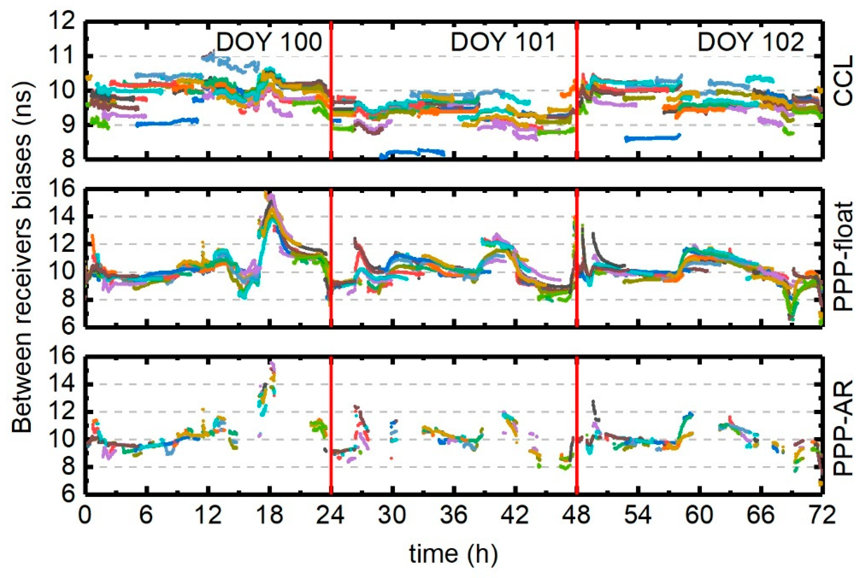
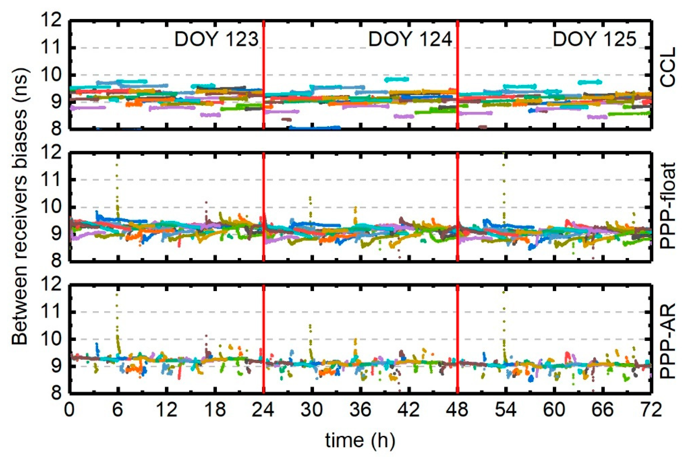
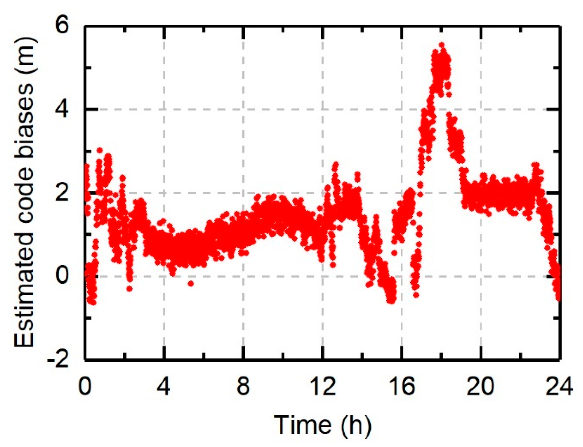
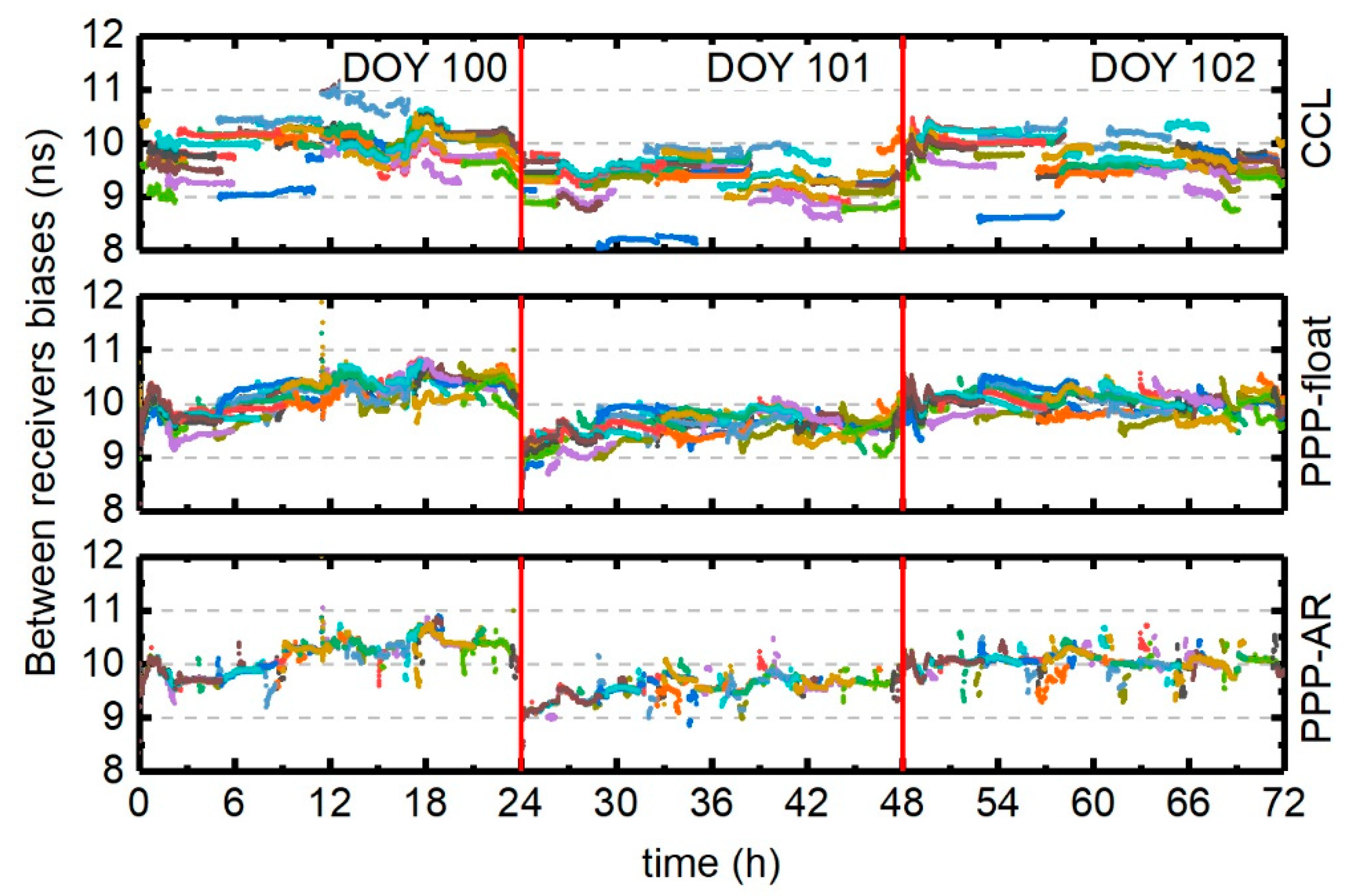
4.1. Analysis of Receiver Biases Variation

4.1.1. Leveling Errors for Analysis of Receiver Biases

Here, the CCL and S-UPPP methods were used to directly extract the ionospheric observables to analyze the BR-DCB by using the stations in Table 2. For Figure 5, the BR-DCBs were estimated with the CCL method, S-UPPP float-ambiguity solutions, and fixed-ambiguity solutions, which are marked as “CCL,” ”PPP-float,” and “PPP-AR,” respectively, over three consecutive days from DOY 100 to 102, 2017. In the CCL solutions, the significant fluctuations in one satellite continuous observation arc indicated that the time-varying amplitude of differential phase biases were noticeable. The main trend also showed the shift of the receiver code bias. In Equation (5), the receiver code bias of each satellite was averaged to remove the multipath effects and fluctuations of the time-varying term. In the CCL method, we could not confirm the details of receiver time-varying code biases. In the S-UPPP method, the ionospheric observables were estimated epoch by an epoch with receiver code bias. For the S-UPPP float solutions, the fluctuation of the BR-DCB is more significant than that in CCL method. In S-UPPP fixed-ambiguity resolution, the ambiguity resolution failed during periods of large variations of code biases. However, as seen in Figure 6, without a large variation of receiver bias, the BR-DCBs in the CCL and S-UPPP solutions was highly consistent and the fixed-ambiguity solutions had the best performance. Compared with the solutions in Figure 6 from DOY 123 to 125, 2017, it can be seen that the fluctuations of the code bias in Figure 5 had clear negative effects for extracting ionospheric delays and ambiguity resolutions in the S-UPPP method. Additionally, the fluctuation of receiver code bias in three consecutive days did not show periodic variations. Some researchers have shown that this variation is caused by local receiver equipment and temperature changes [30,46,47,48].

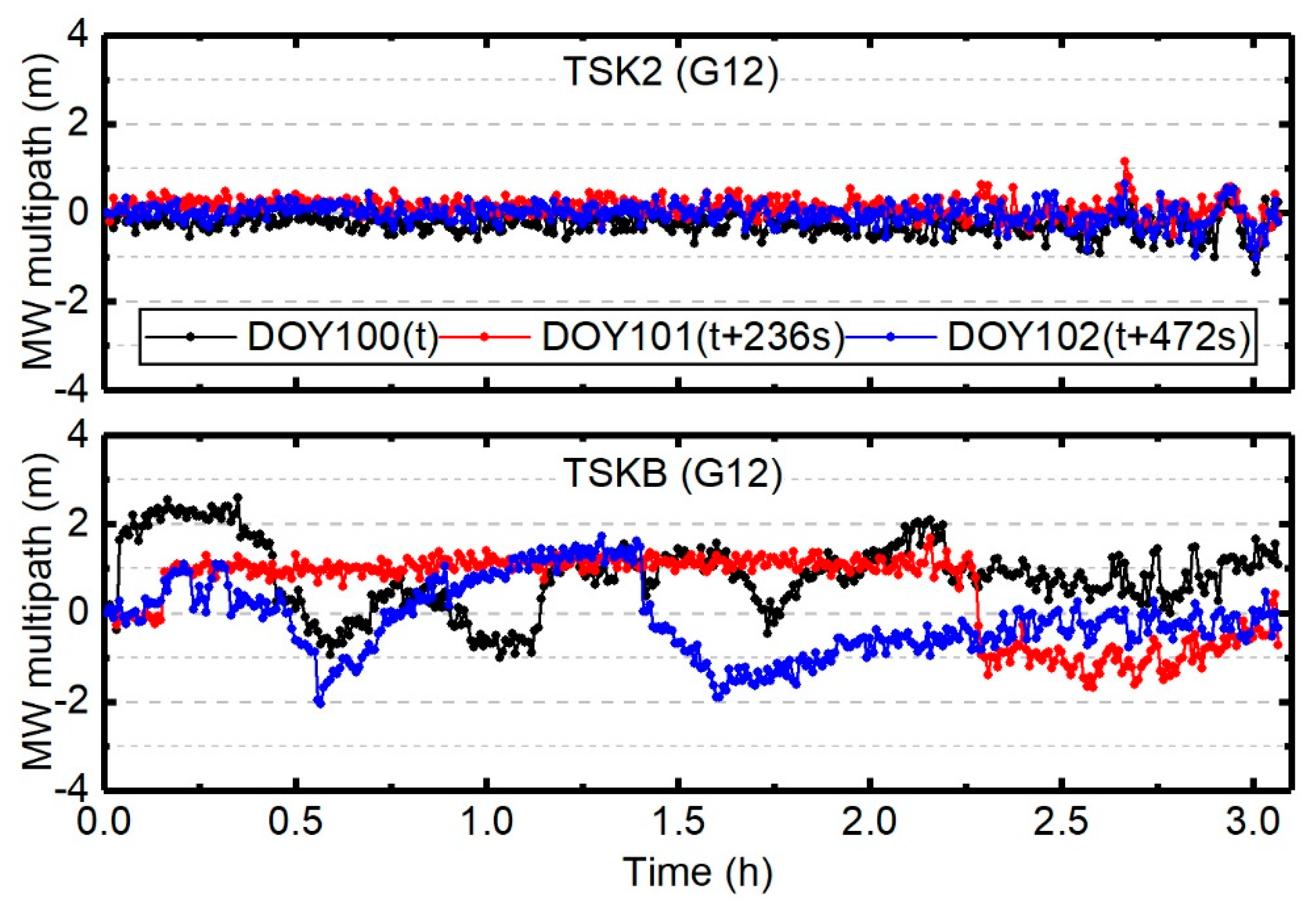
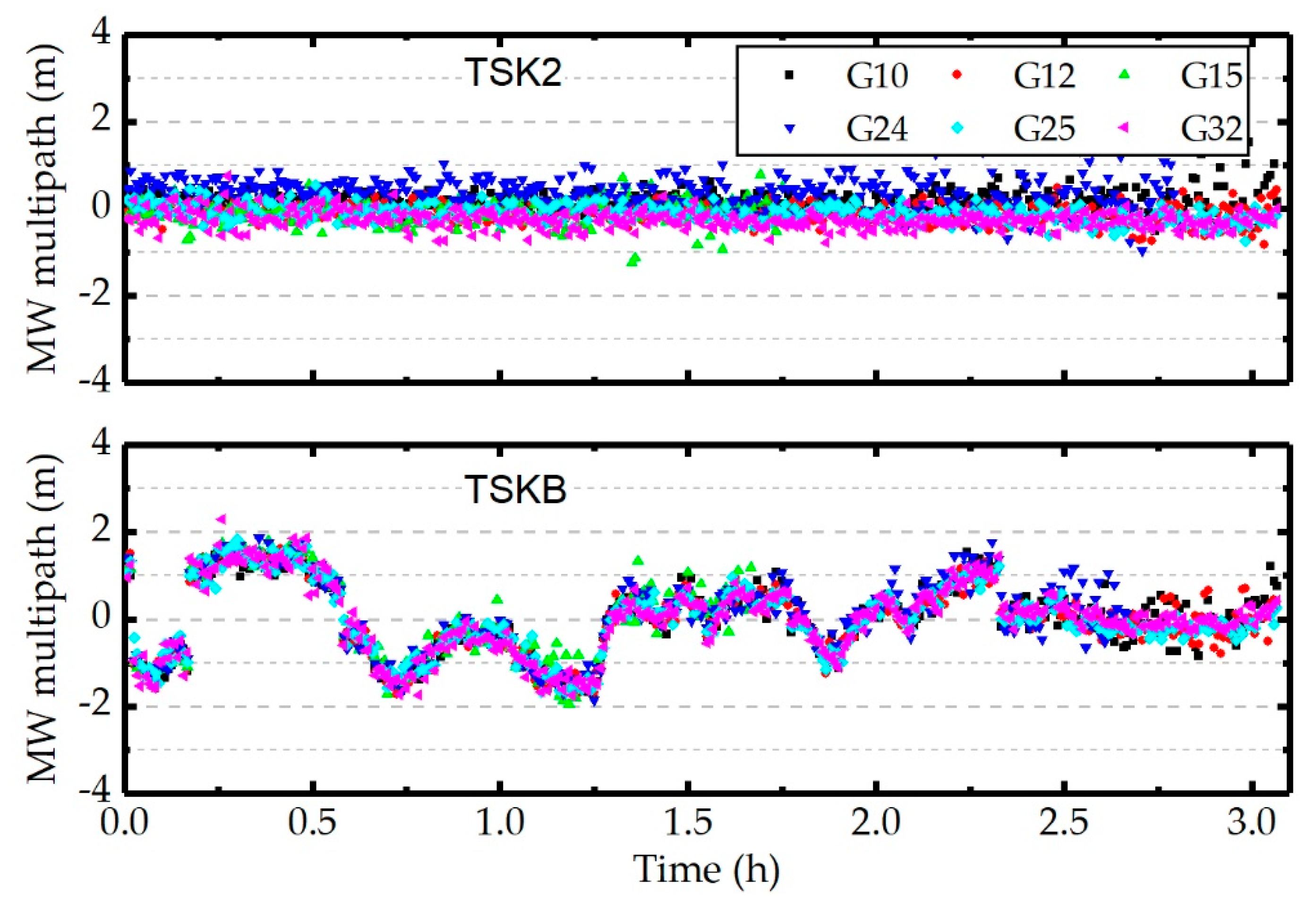
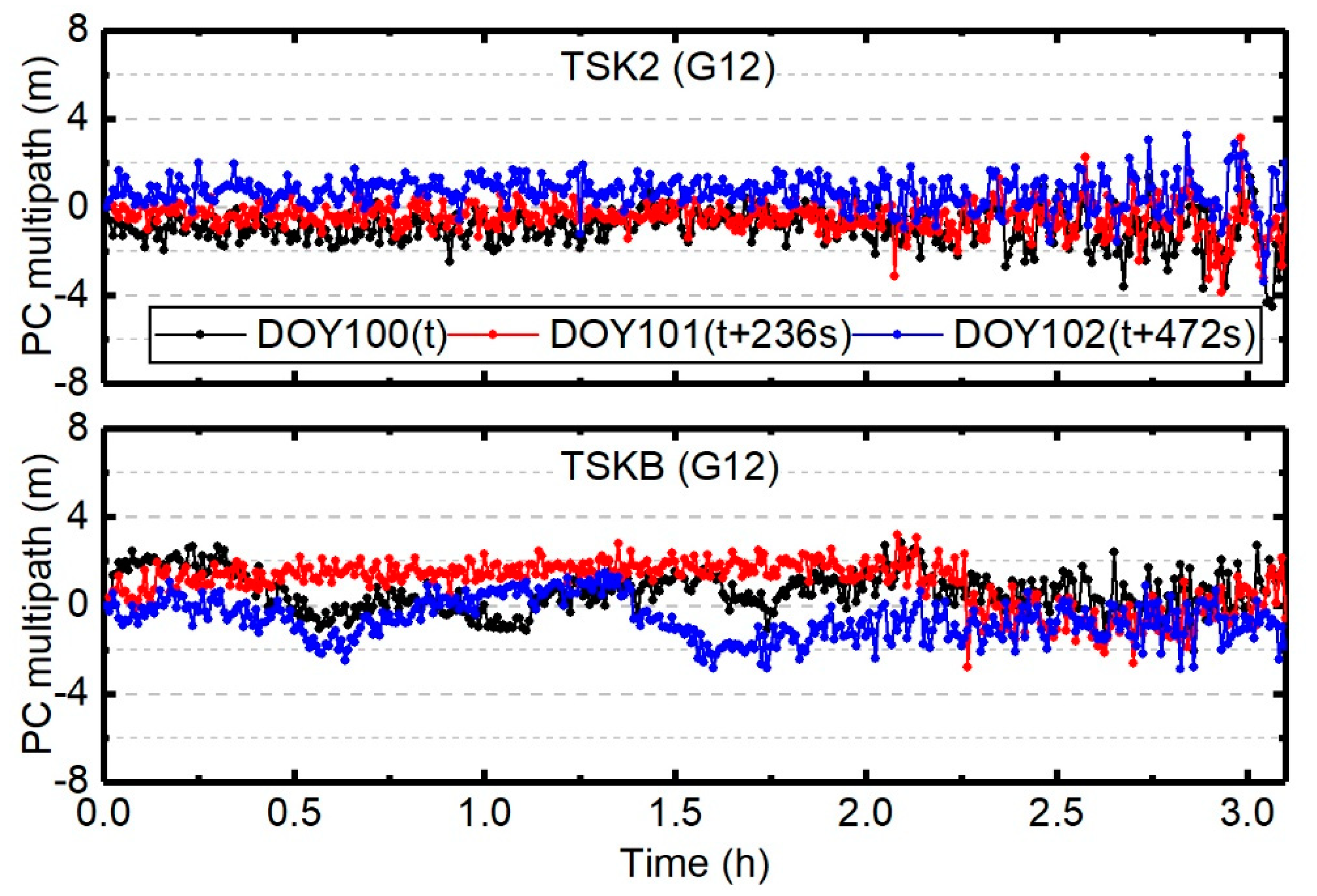
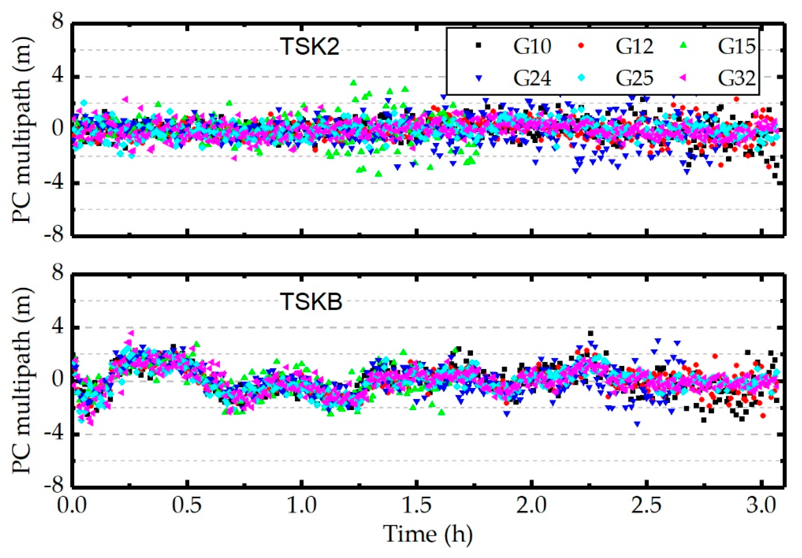
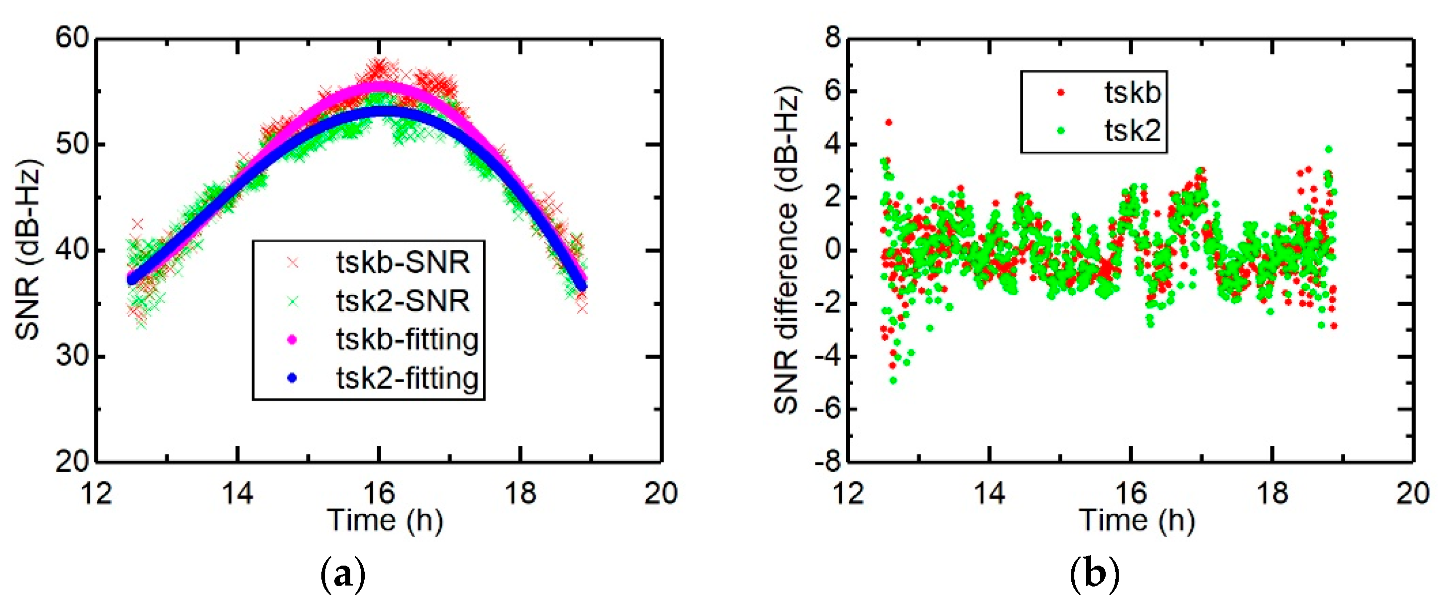
4.1.2. Multipath Analysis

In the CCL method, the BR-DCB is free of the code multipath. Hence, we did not confirm that the DCB variations were mainly caused by the code multipath. Free of ionospheric delays effects, the MW combination in Equation (3) and ionosphere-free combination in Equation (11) were adopted to calculate the code multipath. For Figure 7, the satellite PRN 12 was selected to present the MW code multipath over three consecutive sidereal days in stations TSK2 and TSKB. Compared with TSK2, the MW code multipath results in TSKB with large fluctuation indicated that there must have been some bias in the TSKB code multipath. In Equation (3), this variation may have been caused by the receiver phase and code time-varying terms or the code multipath. The effect of the code multipath was mainly created from certain low-elevation directions. The measurements in this experiment were collected from two static IGS receivers. Therefore, the geometry of the satellite-receiver rays repeated every sidereal day. However, in Figure 7, the station TSKB did not show the MP-repeatability of sidereal days like in the TSK2 results. In Figure 8, six satellite results indicate that this variation must have been a receiver-dependent bias.
In Equation (15), the M-UPPP method was mainly used to remove the ionosphere-free code bias from ambiguities. Hence, the ionosphere-free combination was the proper method to analyze the code bias and the multipath. For Figure 9, the satellite PRN 12 was selected to show the ionosphere-free code multipath over three consecutive days. Similarly, as in the MW combination, the inconsistent fluctuation in TSKB on each sidereal day indicated that the receiver code bias variation must have existed in this multipath. In Figure 10, six satellite results show consistent trends in one day, and these indicated that the receiver-dependent code bias had to be taken into consideration.
Furthermore, to analyze the effect of the multipath errors, signal-to-noise ratio (SNR) measurements were used to analyze the difference between the different receivers. For Figure 11a, the satellite PRN 13 was selected to present the SNR measurements. The major trends could be removed by polynomial fit so that the multipath errors were mainly reflected in the periodic fluctuations of SNR residuals. In Figure 11b, the SNR residuals, after removing the major trends, had the same distributions and variations. At the same time, the two stations had the same satellite distributions with a distance of less than 36.2 m. With the statistical analysis of all satellite in one day, the SNR residuals of all satellites for the two receivers did not have significantly differences. Hence, the variations of the single different ionospheric observables were mainly caused by receiver-dependent code biases.
Similar variations of the single different receiver code biases in Figure 5 have also been found in previous research [24,29,30]. Variations of about 9 ns in [24] and 6.5 ns in [29] for receiver code bias fluctuations within two consecutive hours were already published. Hence, the fluctuation amplitude of receiver code bias depends on receiver-specific conditions, such as hardware version or temperature variations [23]. The effect on positioning of this code bias variations is analyzed in detail in the following.

4.2. The Receiver Biases Effect on PPP with Single Station

The time-varying parts of the code biases are unmodeled errors, a fact that is reflected in the residuals or assimilated into other parameters after adjustment. The TSKB station can be used to analyze the difference between the standard and modified UPPP methods.

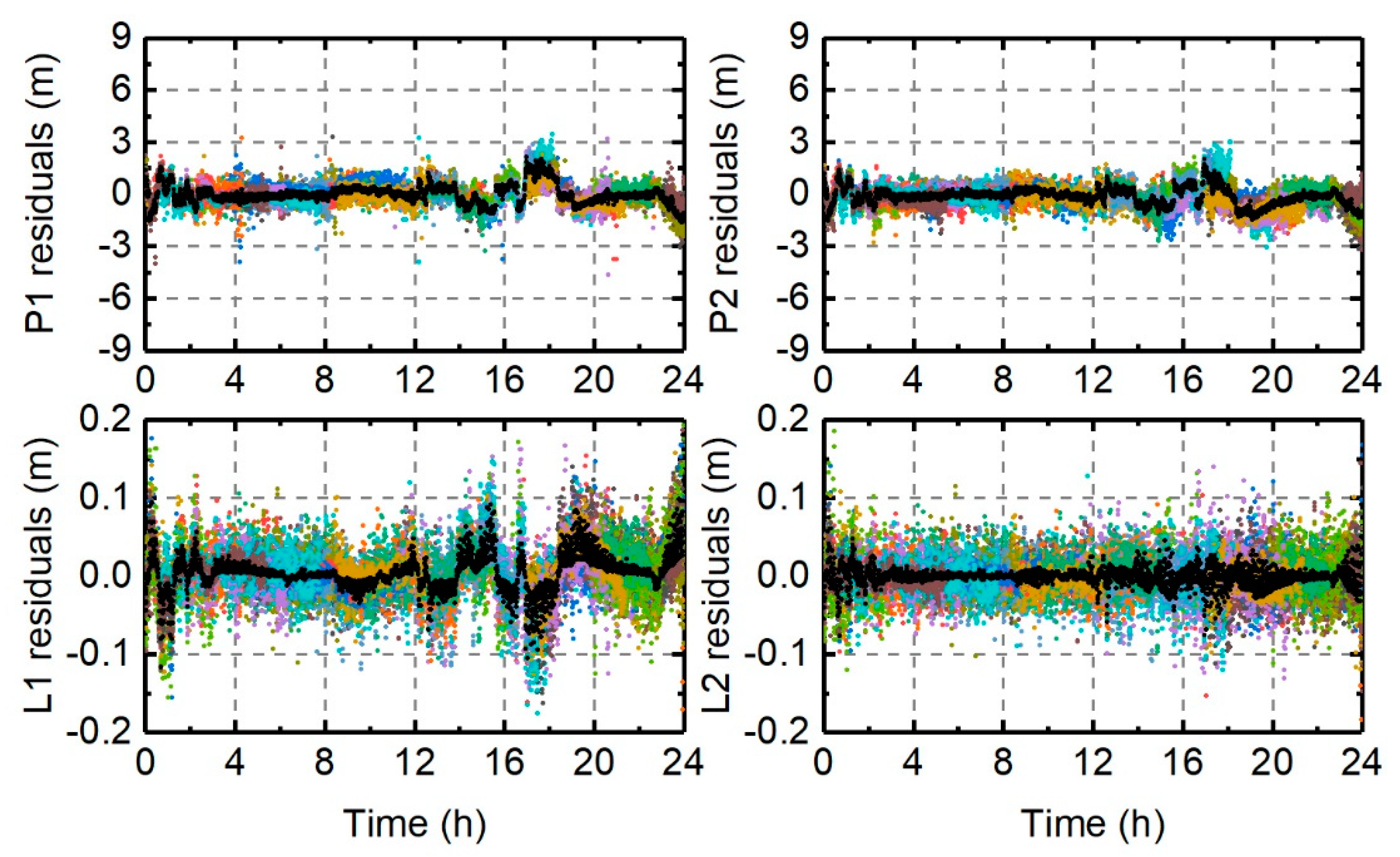
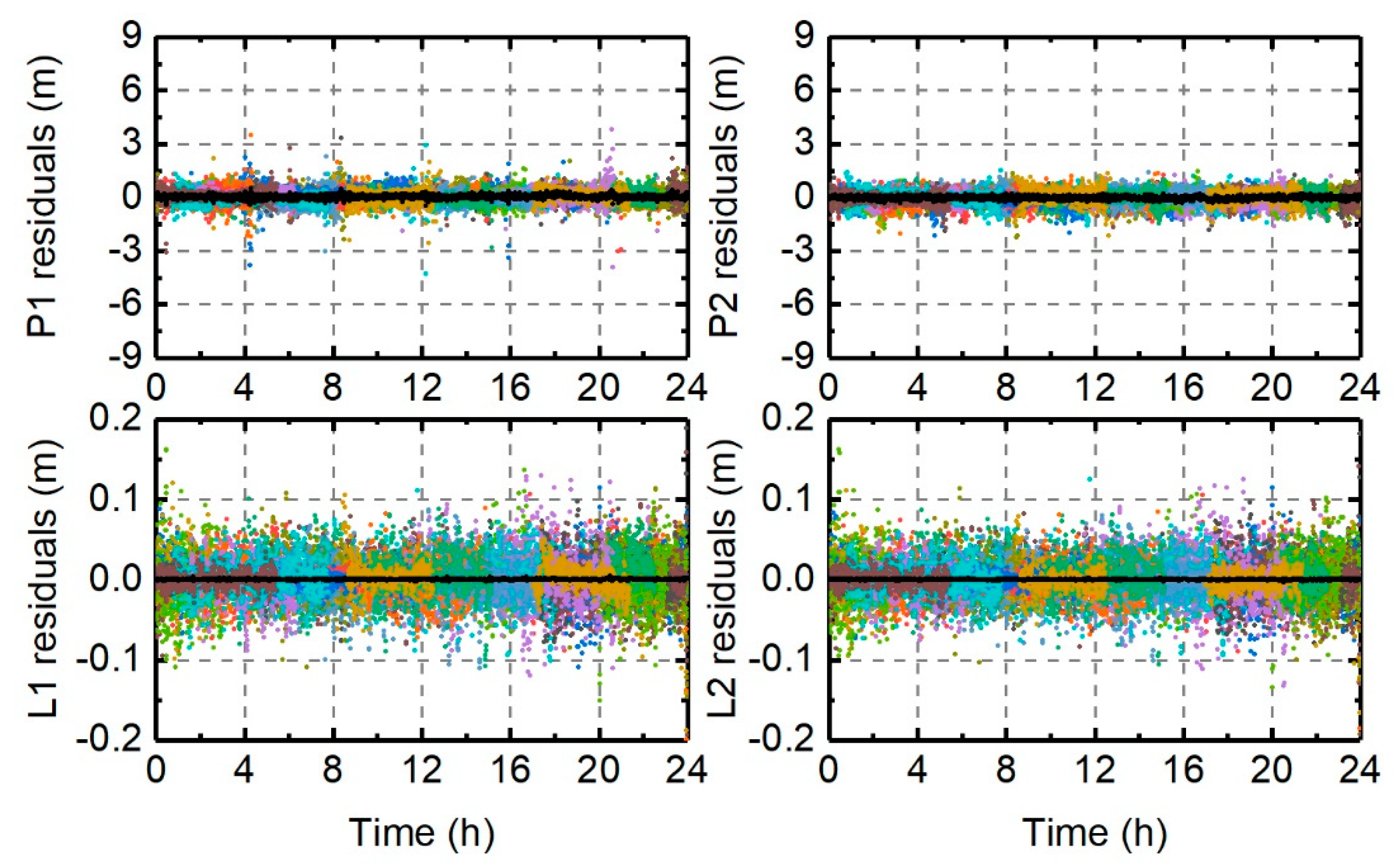
4.2.1. Measurements Residuals

With the assumption that the code biases are constant over time, the S-UPPP model cannot capture the receiver clock offset to a level of accuracy that corresponds to phase observations [49]. The receiver clock offset datum is determined by the code observations, but its accuracy is mainly improved by phase measurements. However, constant combined parameters of ambiguities and code biases cannot represent the variations of code biases over time. Consequentially, the unmodeled errors are assimilated into the residuals, and it is improper to represent combined ambiguity parameters as constants. This is shown in Figure 12.
In the S-UPPP method, the obvious variations in residuals destroyed the Gaussian white noise distribution of the code measurement residuals, although the residuals were expected to be zero-mean. Meanwhile, the abnormal residuals also showed in phase measurements from 16:00 to 20:00 and at the beginning and ending stages. In the M-UPPP method, the unmodeled errors were estimated, and the code and phase residuals had an ideal distribution with zero-mean, as seen in Figure 13.
In Equation (15), the ionosphere-free combined code biases can be directly estimated by M-UPPP. As can be seen in Figure 14, the estimated code biases from the M-UPPP method showed large variations over 4.8 m within two hours, a trend which is the same as in the code residuals of the S-UPPP method. This variation trend is also presented in the BR-DCB of Figure 5. This indicates that the time-varying code bias actually has a negative effect on ambiguity resolution.

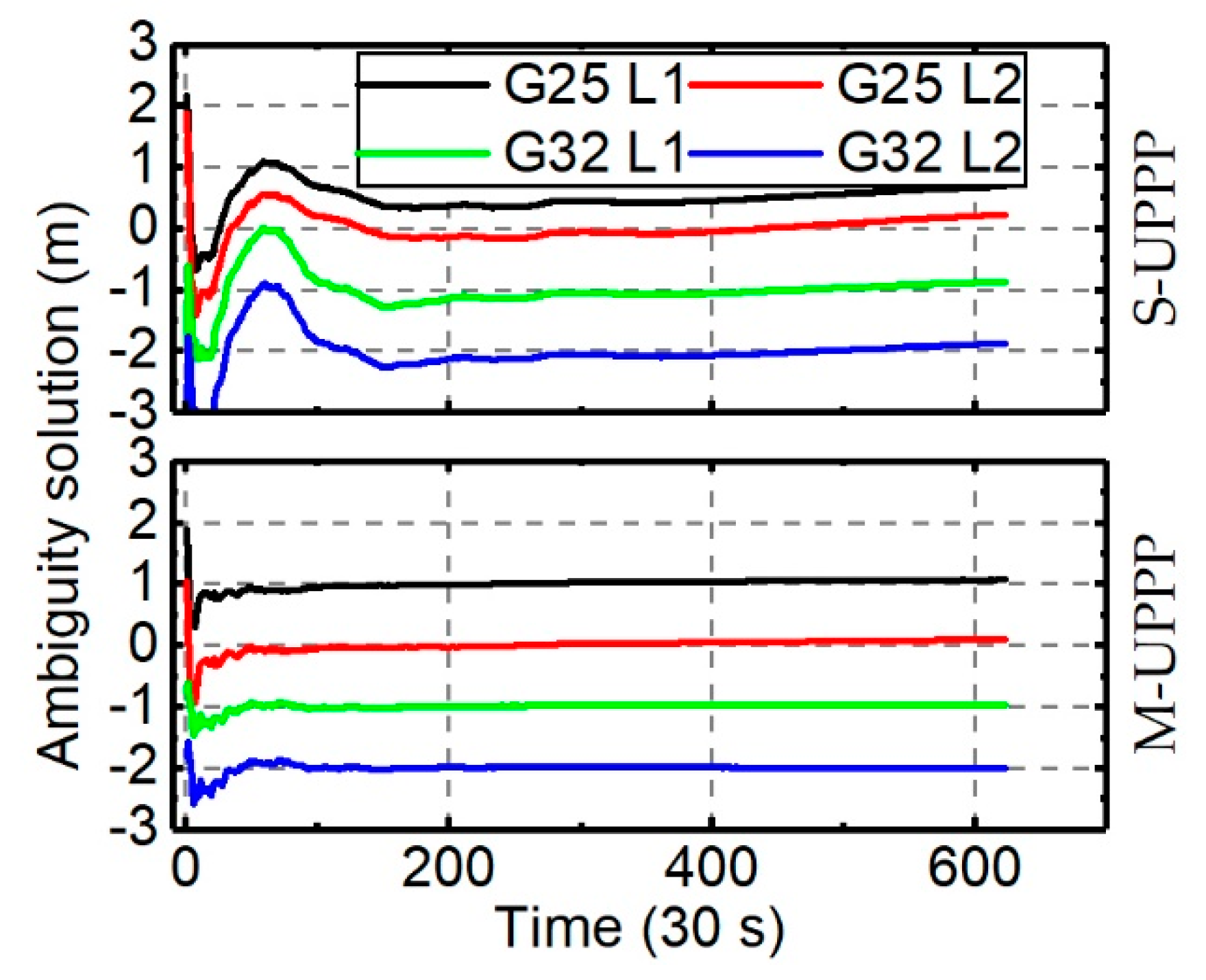
4.2.2. Ambiguity Solutions

At the same time, the isolation of the code biases from ambiguity recovers the strongly stable feature of ambiguities that can be estimated as constant parameters. In Figure 15 (top panel), the large fluctuations represented in the S-UPPP ambiguities of each frequency signal must have hampered the ambiguities to achieve quick convergence. The M-UPPP method enhanced the performance of ambiguities with a constant stable feature in a short time, as shown in Figure 15 (bottom panel).
Firstly, the static positioning improvement on TSKB with the M-UPPP method is shown in Figure 16. The M-UPPP method improved the three-dimensional positioning accuracy from 2.99 to 0.79 cm for the float solution, with a 73.6% improvement, and from 3.17 to 0.85 cm for the fixed solution, with a 73.2% improvement. In the east and up components, large fluctuations vanished in the beginning and at the end of the processing ambiguity float and fixed solutions.
From the static solution, the effects of varying receiver code biases in the UPPP method could be confirmed. These effects were also found in the positioning solutions of the dynamic mode in Figure 17. Significant improvements were found in the M-UPPP method. The large positioning errors were caused by the variation of receiver code biases. The variation of positioning errors was consistent with the variation of the code bias that is shown in Figure 14. The large fluctuations of positioning errors and code bias started at about 16:00. This indicates that the estimation of the ambiguities and coordinate parameters was strongly affected by the large code bias variations in the dynamic positioning mode. Unlike in the static model, the positioning errors were recovered to a regular level along with diminishing receiver code bias variations. The maximum of the positioning errors was about 3.9 m from 16:00 to 20:00.

4.3. Extraction of Ionospheric Observable from M-UPPP

With the above analysis, the accuracy of ionospheric observables that were extracted from the S-UPPP method was degraded by the time-varying receiver code bias. By using the M-UPPP method, we isolated the ionosphere-free combined receiver code bias from ambiguities and ionospheric delays in order to improve the positioning results in TSKB. Hence, the ionospheric observables estimated in the M-UPPP method should be improved. In Figure 18, the new BR-DCB results are presented to illustrate the high consistency between the CCL and M-UPPP methods in extracting the ionospheric observables. Though the time-varying differential phase bias remained in the ionospheric observables, it was quite smaller than the code bias. Additionally, we also obtained the best performance with the ambiguity resolution.

4.4. Receivers Biases Effects on PPP in Statistics Solutions

It has been proven that the M-UPPP method can improve positioning performance in one station, TSKB, from positioning experiments in the static and dynamic modes. To further analyze the effects of this method, we processed all 220 stations for statistic performance.

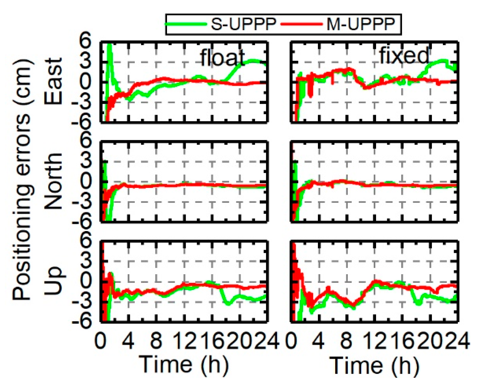
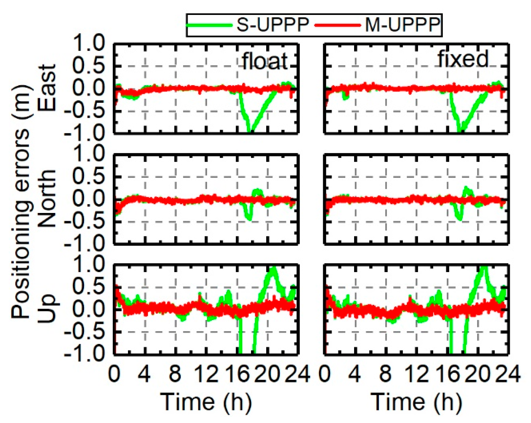
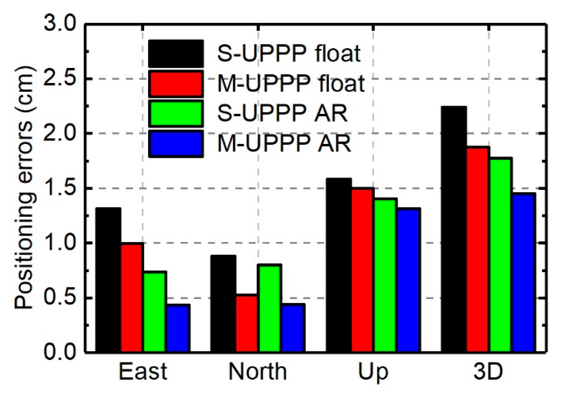
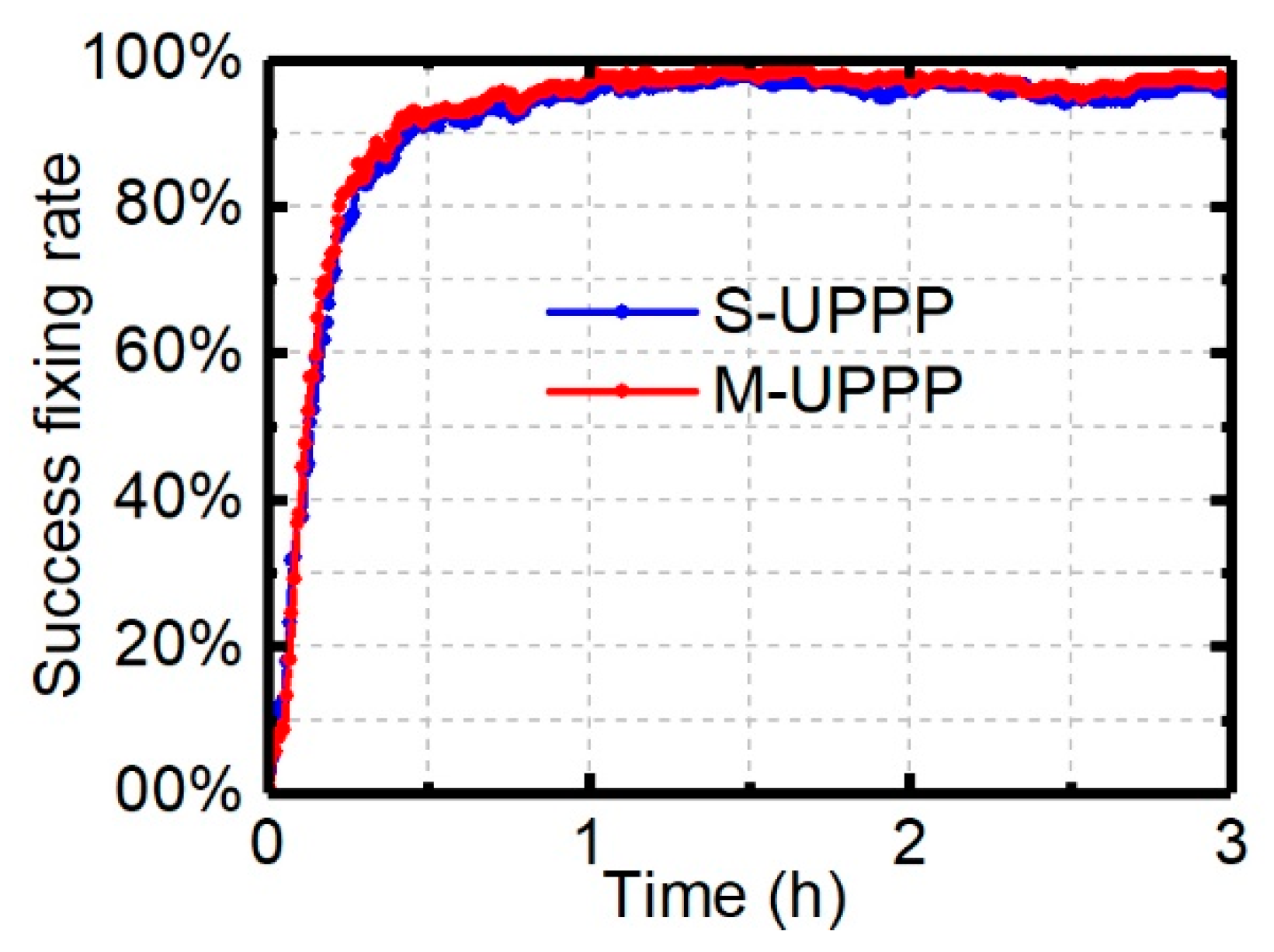
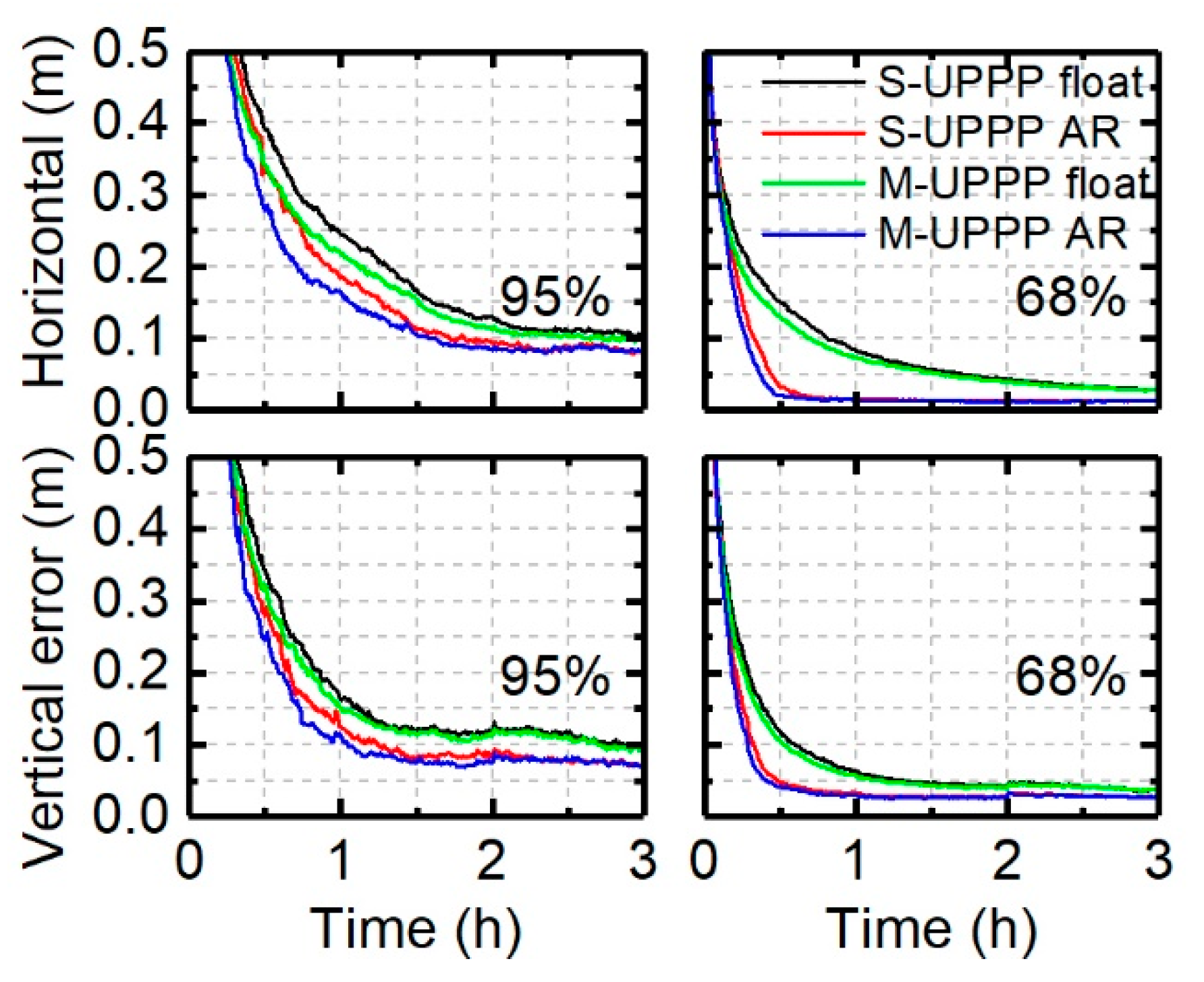
4.4.1. The Performance of Static Positioning

The histogram distribution, which was constructed from the mean value of different UPPP positioning results with a total of 1760 three-hour sessions, is displayed in Figure 19. The significant improvements are presented in the PPP AR, as compared with the float solutions. Compared with the S-UPPP method, the M-UPPP method had significant improvements for the float and fixed ambiguity solutions. The differences between the S-UPPP and M-UPPP methods are presented in Table 3. Compared with the standard UPPP AR, the accuracy was improved from 1.77 to 1.45 cm for the M-UPPP AR.
The positioning performance was evaluated at the 68% and 95% confidence levels in the static PPP model for the S-UPPP and M-UPPP methods in Figure 20. Inevitably, the fixed-ambiguity solutions had higher accuracies than the float solutions in most of periods. Compared with the S-UPPP method, significant improvements could be found over the processing period, especially in the initial phase. Furthermore, the improvements in the horizontal component were more significant than those in the vertical component. With the modified methods, a fast convergence could be achieved for the fixed-ambiguity solutions.
The ambiguity fixing success rate is defined as the ratio of the number of the fixed solutions to that of all solutions in one epoch. The fixed-ambiguity resolution in one epoch can be confirmed by a ambiguity resolution ratio that is larger than 2 and a difference of the absolute fixed positioning errors minus the float positioning errors of less than 3 cm. In Figure 21, similar slight improvements are presented for UPPP methods. In Table 4, the significant improvements in terms of convergence time are presented. Here, we define the convergence time as to when the averaged three-dimensional RMS was smaller than 10 cm in the static mode, smaller than 20 cm in the dynamic mode, and lasting for 10 continuous epochs [18,50,51]. Compared with the S-UPPP methods with the fixed-ambiguity solutions in which the convergence times were 90 and 17 min under the 95% and 68% confidence levels, it took 43 and 14 min for the M-UPPP method to converge to the defined accuracy. The convergence times of the float solutions were 111 and 36 min for the S-UPPP method and 81.5 and 31 min for the M-UPPP method under the 95% and 68% confidence levels, respectively. The M-UPPP method significantly improved the static positioning accuracy and shortened the convergence time.

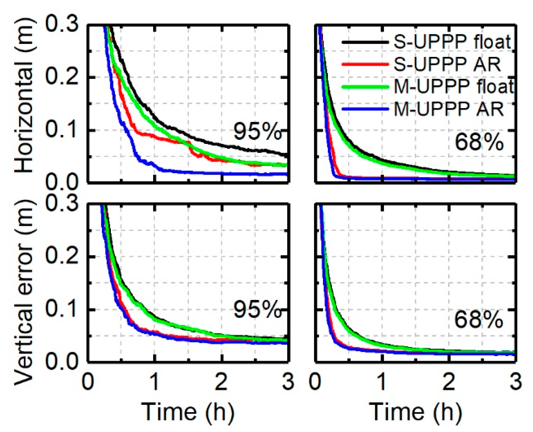
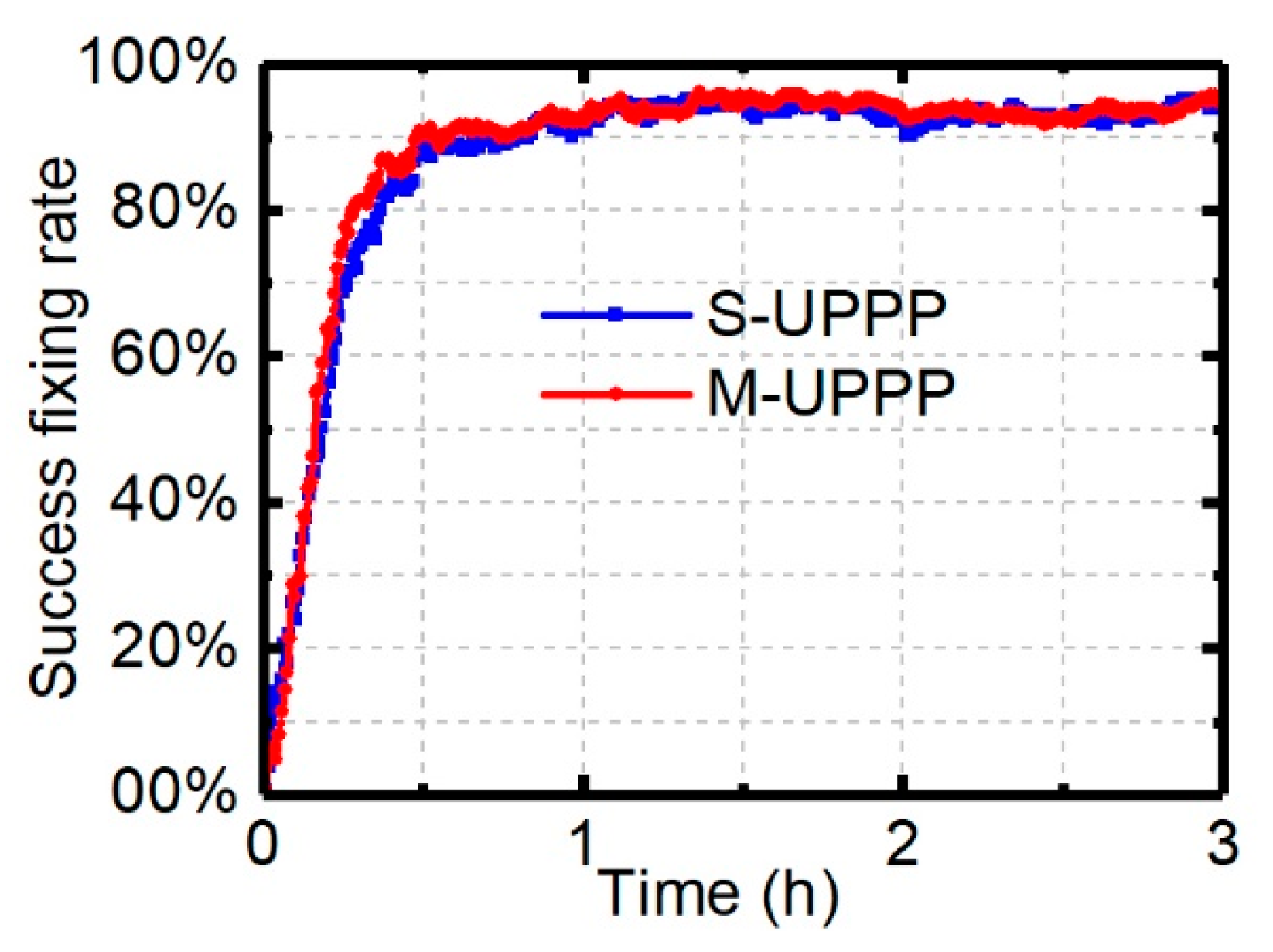
4.4.2. The Positioning Performance in Dynamic Mode

The dynamic experiments were processed with same data as in static experiments. Similar improvements to those in the static mode are presented in Figure 22. The improvement in the horizontal component was more significant than that in the vertical component. Slight improvements are also presented in Figure 23 for the M-UPPP method. The improvements in terms of convergence time are also shown in Table 5. For the dynamic mode, the threshold value of the convergence time was defined as 20 cm. Compared with the S-UPPP methods with the fixed-ambiguity solutions in which the convergence times were 70.5 and 20 min under the 95% and 68% confidence levels, it took 55.5 and 16 min for the M-UPPP method to converge to the defined accuracy, respectively. The convergence times of the float solutions were 89.5 and 34.5 min for the S-UPPP method and 77 and 28 min for the M-UPPP method under the 95% and 68% confidence levels, respectively. The M-UPPP method also significantly improved the dynamic positioning accuracy and shortened the convergence time.

5. Discussion

A high precision ambiguity solution is the main goal of ambiguity resolution in the PPP AR. In this study, we focused on the effect of receiver code biases in ambiguity resolution. With more reliable and stable ambiguity solutions, a faster PPP AR was achieved with a higher ambiguity fixing success rate. Long-term and short-term variations of receiver code biases have been demonstrated [23,24,29,30,31,35,36]. Due to the difficulty in the isolation of receiver code biases from observables and their receiver-dependent features, many researchers have not studied their absolute values and their effects on positioning performance. With the introduced method, the variation of receiver code bias can be directly estimated. Its effects on ambiguity resolution can be removed, which benefits the PPP AR. In Figure 10, it can be seen that variation of code bias was up to 4.8 m within the two-hour data for the PPP AR. After removing the code bias, the ambiguity parameters quickly achieved stable solutions. The improved performance of positioning could be found in the static and dynamic modes for the M-UPPP method. The variations of receiver code bias are dependent on the quality of equipment and on location environment. The effect of code bias on a single receiver is detailed here to present the effective performance of eliminating the effect of receiver code bias on positioning and ambiguity resolution. This method has been confirmed that it is effective in static and dynamic mode for PPP. Hence, the performance of the PPP AR in real-time applications should be further studied in next work.

6. Conclusions

This study introduced a modified method to mitigate the short-term temporal variations of receiver code bias for an increased ambiguity success fixing rate in PPP and improving positioning performance. We decoupled the receiver clock offset parameters with ambiguities and isolated the code biases from ambiguities. The effects of code biases can be removed from ambiguities, and the integer nature of ambiguities are easier to be recovered. We performed experiments by using the standard and modified methods in the UPPP model to present the code biases and evaluate the improvement in terms of convergence time and success rate of ambiguity resolution in static and dynamic PPP.
Based on the analysis of the measurement residuals, remarkable short-term temporal variations of the code biases up to 16 ns within two hours have been detected. These unmodeled errors also affect the phase measurement residuals. With the improved method, the code biases are removed from ambiguities and the ambiguities become more stable. For some special stations, the improvement of the positioning accuracy for the ambiguity float and fixed solutions is significant. It is valuable to rigorously take variations of code biases into consideration in UPPP processing.
With the observations from the IGS network, the improvement in terms of convergence time and success rate of ambiguity resolution are presented. Significant improvements of final ambiguity-float and ambiguity-fixed solutions for the M-UPPP method were achieved with three-hour data. In the S-UPPP method, the convergence times were 36 and 17 min for ambiguity float and fixed solutions, respectively, and these were 31 and 14 min in the M-UPPP method under the 68% confidence level. Higher ambiguity fixing success rates were also achieved at different times for the M-UPPP method. Under the 95% confidence level, the same trends are also clearly presented. By the dynamic PPP processing, similar improvements were found for the M-UPPP method. Hence, the improvement was significant for isolating the code biases from ambiguities and crucial to achieving a rapid ambiguity-fixed solution. When it comes to using the satellite clock offsets and phase biases products, the effects of code biases in network solutions should also be taken into heavier consideration, as will be done in future work.

Author Contributions

J.W., G.H. and P.Z. conceived and designed the experiments; J.W. performed the experiments, analyzed the data and wrote the paper; Y.Y., Q.Z. and Y.G. reviewed the paper. All authors have read and agreed to the published version of the manuscript.

Acknowledgments

This work was supported by the National Key Research and Development Program of China (2018YFC1505102), the Programs of the National Natural Science Foundation of China (41774025, 41731066, 41904039), Special Fund for Technological Innovation Guidance of Shaanxi Province (2018XNCGG05), the Special Fund for Basic Scientific Research of Central Colleges (Grant No. CHD300102269305, CHD300102268305, Chang’an University), the Grand Projects of the Beidou-2 System (GFZX0301040308) and the China Scholarship Council (award to Jin Wang for 2 year’s study abroad at the University of Calgary). We also thank the IGS and iGMAS authorities for providing the data for this study.

Conflicts of Interest

The authors declare no conflict of interest.

References

  1. Gabor, M.J.; Nerem, R.S. GPS Carrier Phase Ambiguity Resolution Using Satellite-Satellite Single Differences. In Proceedings of the ION GNSS 1999, Institute of Navigation, Nashville, TN, USA, 14–17 September 1999; pp. 1569–1578. [Google Scholar]
  2. Ge, M.; Gendt, G.; Rothacher, M.; Shi, C.; Liu, J. Resolution of GPS carrier-phase ambiguities in Precise Point Positioning (PPP) with daily observations. J. Geod. 2008, 82, 389–399. [Google Scholar] [CrossRef]
  3. Geng, J.; Teferle, F.N.; Shi, C.; Meng, X.; Dodson, A.H.; Liu, J. Ambiguity resolution in precise point positioning with hourly data. GPS Solut. 2009, 13, 263–270. [Google Scholar] [CrossRef] [Green Version]
  4. Li, X.; Ge, M.; Zhang, H.; Wickert, J. A method for improving uncalibrated phase delay estimation and ambiguity-fixing in real-time precise point positioning. J. Geod. 2013, 87, 405–416. [Google Scholar] [CrossRef]
  5. Laurichesse, D.; Mercier, F.; Berthias, J.P.; Bijac, J. Real Time Zero-difference Ambiguities Fixing and Absolute RTK. In Proceedings of the 2008 National Technical Meeting, The Institute of Navigation, San Diego, CA, USA, 28–30 January 2008; pp. 747–755. [Google Scholar]
  6. Collins, P.; Lahaye, F.; Heroux, P.; Bisnath, S. Precise Point Positioning with Ambiguity Resolution using the Decoupled Clock Model. In Proceedings of the ION GNSS 2008, Institute of Navigation, Savannah, GA, USA, 16–19 September 2008; pp. 1315–1322. [Google Scholar]
  7. Li, X.; Li, X.; Yuan, Y.; Zhang, K.; Zhang, X.; Wickert, J. Multi-GNSS phase delay estimation and PPP ambiguity resolution: GPS, BDS, GLONASS, Galileo. J. Geod. 2017, 92, 579–608. [Google Scholar] [CrossRef]
  8. Li, P.; Zhang, X.; Ren, X.; Zuo, X.; Pan, Y. Generating GPS satellite fractional cycle bias for ambiguity-fixed precise point positioning. GPS Solut. 2016, 20, 771–782. [Google Scholar] [CrossRef]
  9. Xiao, G.; Sui, L.; Heck, B.; Zeng, T.; Tian, Y. Estimating satellite phase fractional cycle biases based on Kalman filter. GPS Solut. 2018, 22, 82. [Google Scholar] [CrossRef]
  10. Wang, J.; Huang, G.; Yang, Y.; Zhang, Q.; Gao, Y.; Xiao, G. FCB estimation with three different PPP models: Equivalence analysis and experiment tests. GPS Solut. 2019, 23, 93. [Google Scholar] [CrossRef]
  11. Odijk, D.; Zhang, B.; Khodabandeh, A.; Odolinski, R.; Teunissen, P.J.G. On the estimability of parameters in undifferenced, uncombined GNSS network and PPP-RTK user models by means of S-system theory. J. Geod. 2016, 90, 15–44. [Google Scholar] [CrossRef]
  12. Teunissen, P.J.G.; Khodabandeh, A. Review and principles of PPP-RTK methods. J. Geod. 2015, 89, 217–240. [Google Scholar] [CrossRef]
  13. Teunissen, P.J.G.; Kleusberg, A. GPS for Geodesy, 2rd ed.; Springer: Berlin, Germany, 1998; pp. 188–194. [Google Scholar]
  14. Wang, M.; Gao, Y. An Investigation on GPS Receiver Initial Phase Bias and Its Determination. In Proceedings of the ION NTM 2007, The Institute of Navigation, San Diego, CA, USA, 22–24 January 2007; pp. 873–880. [Google Scholar]
  15. Kouba, J.; Héroux, P. Precise Point Positioning Using IGS Orbit and Clock Products. GPS Solut. 2001, 5, 12–28. [Google Scholar] [CrossRef]
  16. Geng, J.; Meng, X.; Dodson, A.H.; Teferle, F.N. Integer ambiguity resolution in precise point positioning: Method comparison. J. Geod. 2010, 84, 569–581. [Google Scholar] [CrossRef] [Green Version]
  17. Zhang, B.; Chen, Y.; Yuan, Y. PPP-RTK based on undifferenced and uncombined observations: Theoretical and practical aspects. J. Geod. 2018, 93, 1011–1024. [Google Scholar] [CrossRef]
  18. Zhou, F.; Dong, D.; Li, W.; Jiang, X.; Wickert, J.; Schuh, H. GAMP: An open-source software of multi-GNSS precise point positioning using undifferenced and uncombined observations. GPS Solut. 2018, 22, 23. [Google Scholar] [CrossRef]
  19. Fu, W.; Huang, G.; Zhang, Q.; Gu, S.; Ge, M.; Schuh, H. Multi-GNSS real-time clock estimation using sequential least square adjustment with online quality control. J. Geod. 2018, 93, 963–976. [Google Scholar] [CrossRef]
  20. Huang, G.; Cui, B.; Zhang, Q.; Fu, W.; Li, P. An Improved Predicted Model for BDS Ultra-Rapid Satellite Clock Offsets. Remote Sens. 2018, 10, 60. [Google Scholar] [CrossRef] [Green Version]
  21. Huang, G.; Yan, X.; Zhang, Q.; Liu, C.; Wang, L.; Qin, Z. Estimation of antenna phase center offset for BDS IGSO and MEO satellites. GPS Solut. 2018, 22, 49. [Google Scholar] [CrossRef]
  22. Hernández-Pajares, M.; Juan, J.M.; Sanz, J.; Orus, R.; Garcia-Rigo, A.; Feltens, J.; Komjathy, A.; Schaer, S.C.; Krankowski, A. The IGS VTEC maps: A reliable source of ionospheric information since 1998. J. Geod. 2009, 83, 263–275. [Google Scholar] [CrossRef]
  23. Wang, N.; Yuan, Y.; Li, Z.; Montenbruck, O.; Tian, B. Determination of differential code biases with multi-GNSS observations. J. Geod. 2016, 90, 209–228. [Google Scholar] [CrossRef]
  24. Li, M.; Yuan, Y.; Wang, N.; Liu, T.; Chen, Y. Estimation and analysis of the short-term variations of multi-GNSS receiver differential code biases using global ionosphere maps. J. Geod. 2018, 92, 889–903. [Google Scholar] [CrossRef]
  25. Sardón, E.; Zarraoa, N. Estimation of total electron content using GPS data: How stable are the differential satellite and receiver instrumental biases? Radio Sci. 1997, 32, 1899–1910. [Google Scholar] [CrossRef]
  26. Zhang, B.; Teunissen, P.J.G. Characterization of multi-GNSS between-receiver differential code biases using zero and short baselines. Sci. Bull. 2015, 60, 1840–1849. [Google Scholar] [CrossRef] [Green Version]
  27. Li, M.; Yuan, Y.; Wang, N.; Li, Z.; Li, Y.; Huo, X. Estimation and analysis of Galileo differential code biases. J. Geod. 2017, 91, 279–293. [Google Scholar] [CrossRef]
  28. Sanz, J.; Juan, J.M.; Rovira-Garcia, A.; González-Casado, G. GPS differential code biases determination: Methodology and analysis. GPS Solut. 2017, 21, 1549–1561. [Google Scholar] [CrossRef] [Green Version]
  29. Zhang, B.; Teunissen, P.J.G.; Yuan, Y. On the short-term temporal variations of GNSS receiver differential phase biases. J. Geod. 2017, 91, 563–572. [Google Scholar] [CrossRef] [Green Version]
  30. Zha, J.; Zhang, B.; Yuan, Y.; Zhang, X.; Li, M. Use of modified carrier-to-code leveling to analyze temperature dependence of multi-GNSS receiver DCB and to retrieve ionospheric TEC. GPS Solut. 2019, 23, 103. [Google Scholar] [CrossRef]
  31. Zhang, B.; Teunissen, P.J.G.; Yuan, Y.; Zhang, X.; Li, M. A modified carrier-to-code leveling method for retrieving ionospheric observables and detecting short-term temporal variability of receiver differential code biases. J. Geod. 2018, 93, 19–28. [Google Scholar] [CrossRef] [Green Version]
  32. Chen, L.; Yi, W.; Song, W.; Shi, C.; Lou, Y.; Cao, C. Evaluation of three ionospheric delay computation methods for ground-based GNSS receivers. GPS Solut. 2018, 22, 125. [Google Scholar] [CrossRef]
  33. Zhang, B. The Theory and Application Study of GNSS Undifferenced and Uncombined Precise Point Positioning. Ph.D. Thesis, Chinese Academy of Sciences, Wuhan, China, 2012. [Google Scholar]
  34. Shi, J.; Gao, Y. A comparison of three PPP integer ambiguity resolution methods. GPS Solut. 2014, 18, 519–528. [Google Scholar] [CrossRef]
  35. Kao, S.; Tu, Y.; Chen, W.; Weng, D.J.; Ji, S.Y. Factors affecting the estimation of GPS receiver instrumental biases. Surv. Rev. 2012, 45, 59–67. [Google Scholar] [CrossRef]
  36. Mohamed, A.; Ahmed, E.R. MGR-DCB: A precise model for multi-constellation GNSS receiver differential code bias. J. Navig. 2016, 69, 698–708. [Google Scholar] [CrossRef] [Green Version]
  37. Sanz, S.J.; Juan, Z.J.; Hernández-Pajares, M. GNSS Measurements and Data Preprocessing. In GNSS Data Processing; ESA Communications: Paris, France, 2013; Volume 1, pp. 77–78. [Google Scholar]
  38. Xiang, Y.; Gao, Y.; Shi, J.; Xu, C. Consistency and analysis of ionospheric observables obtained from three precise point positioning models. J. Geod. 2019, 93, 1161–1170. [Google Scholar] [CrossRef]
  39. Guo, J.; Geng, J. GPS satellite clock determination in case of inter-frequency clock biases for triple-frequency precise point positioning. J. Geod. 2018, 92, 1133–1142. [Google Scholar] [CrossRef]
  40. Zhang, H.; Gao, Z.; Ge, M.; Niu, X.; Huang, L.; Tu, R.; Li, X. On the Convergence of Ionospheric Constrained Precise Point Positioning (IC-PPP) Based on Undifferential Uncombined Raw GNSS Observations. Sensors 2013, 13, 15708–15725. [Google Scholar] [CrossRef] [PubMed] [Green Version]
  41. Li, P.; Zhang, X.; Ge, M.; Schuh, H. Three-frequency BDS precise point positioning ambiguity resolution based on raw observables. J. Geod. 2018, 92, 1357–1369. [Google Scholar] [CrossRef] [Green Version]
  42. Teunissen, P.J.G. The least-squares ambiguity decorrelation adjustment: A method for fast GPS integer ambiguity estimation. J. Geod. 1995, 70, 65–82. [Google Scholar] [CrossRef]
  43. Verhagen, S.; Teunissen, P.J.G. The ratio test for future GNSS ambiguity resolution. GPS Solut. 2013, 17, 535–548. [Google Scholar] [CrossRef]
  44. Li, P.; Zhang, X. Precise Point Positioning with Partial Ambiguity Fixing. Sensors 2015, 15, 13627–13643. [Google Scholar] [CrossRef] [Green Version]
  45. Geng, J.; Chen, X.; Pan, Y.; Zhao, Q. A modified phase clock/bias model to improve PPP ambiguity resolution at Wuhan University. J. Geod. 2019, 93, 2053–2067. [Google Scholar] [CrossRef]
  46. Mylnikova, A.A.; Yasyukevich, Y.V.; Kunitsyn, V.E.; Padokhin, A.M. Variability of GPS/GLONASS differential code biases. Results Phys. 2015, 5, 9–10. [Google Scholar] [CrossRef] [Green Version]
  47. Themens, D.R.; Jayachandran, P.T.; Langley, R.B. The nature of GPS differential receiver bias variability: An examination in the polar cap region. J. Geophys. Res. Space Phys. 2015, 120, 8155–8175. [Google Scholar] [CrossRef]
  48. Choi, B.-K.; Lee, S.J. The influence of grounding on GPS receiver differential code biases. Adv. Space Res. 2018, 62, 457–463. [Google Scholar] [CrossRef]
  49. Collins, P.; Bisnath, S.; Lahaye, F.; Héroux, P. Undifferenced GPS Ambiguity Resolution Using the Decoupled Clock Model and Ambiguity Datum Fixing. Navigation 2010, 57, 123–135. [Google Scholar] [CrossRef] [Green Version]
  50. Li, P.; Zhang, X. Integrating GPS and GLONASS to accelerate convergence and initialization times of precise point positioning. GPS Solut. 2014, 18, 461–471. [Google Scholar] [CrossRef]
  51. Lou, Y.; Zheng, F.; Gu, S.; Wang, C.; Guo, H.; Feng, Y. Multi-GNSS precise point positioning with raw single-frequency and dual-frequency measurement models. GPS Solut. 2016, 20, 849–862. [Google Scholar] [CrossRef]
Figure 1. Distribution of reference stations for fractional-cycle biases (FCB) estimation; 162 stations were chosen from the International GNSS (global navigation satellite system) Service (IGS) network as reference stations at the server end.
Remotesensing 12 00796 g001
Figure 2. Flowchart of FCB estimation based on the undifferenced and uncombined precise point positioning (PPP) method.
Remotesensing 12 00796 g002
Figure 3. Disturbance storm index (Dst) (a) and Kp index (b) to indicate the geomagnetic activity during the period of 10 April 2017 (DOY 100, 2017).
Remotesensing 12 00796 g003
Figure 4. Distribution of stations: 220 stations were chosen from the IGS network, excluding the stations in the reference network of the FCB estimation.
Remotesensing 12 00796 g004
Figure 5. Ionospheric biases between two receivers, TSKB and TSK2, from DOY 100 to 102, 2017 with carrier-to-code leveling (CCL) (top), PPP float (middle), and ambiguity resolved (bottom) solutions. The three day solutions are distinguished by red vertical lines. The colored dots indicate individual satellite biases.
Remotesensing 12 00796 g005
Figure 6. Ionospheric biases between two receivers, TSKB and TSK2, from DOY 123 to 125, 2017 with the CCL (top), PPP float (middle) and ambiguity resolved (bottom) solutions. The three day solutions are distinguished by red vertical lines. The colored dots indicate individual satellite biases.
Remotesensing 12 00796 g006
Figure 7. Multipath repeatability of satellite G12 Melbourne–Wübbena (MW) combinations (average reduced) in TSK2 (top) and TSKB (bottom) over three consecutive sidereal days from DOY 100 to 102, 2017. Note that datasets with 30 s samples were adapted to the plot. Actually, the time difference between two consecutive sidereal days was 240 s. The following is the same.
Remotesensing 12 00796 g007
Figure 8. Multipath of the MW combinations (average reduced) in TSK2 (top) and TSKB (bottom) with all observed satellites on DOY 100, 2017.
Remotesensing 12 00796 g008
Figure 9. Multipath repeatability of satellite G12 LC minus PC (average reduced) in TSK2 (top) and TSKB (bottom) over three consecutive sidereal days from DOY 100 to 102, 2017.
Remotesensing 12 00796 g009
Figure 10. Multipath of LC minus PC combinations (average reduced) in TSK2 (top) and TSKB (bottom) with all observed satellites on DOY 100, 2017.
Remotesensing 12 00796 g010
Figure 11. The signal-to-noise ratio (SNR) measurements (a) and their residuals after removing the major trends (b) for satellite PRN 13 of TSKB and TSK2.
Remotesensing 12 00796 g011
Figure 12. Residuals of the standard uncombined PPP (S-UPPP) method for code (top) and phase (bottom) measurements of two frequency signals. The black points are the averaged epoch residuals, and the colored dots indicate individual satellite residuals.
Remotesensing 12 00796 g012
Figure 13. Residuals of the modified UPPP (M-UPPP) method for code (top) and phase (bottom) measurements of two frequency signals. The black points are the averaged epoch residuals, and the colored dots indicate individual satellite residuals.
Remotesensing 12 00796 g013
Figure 14. Code biases estimated from the M-UPPP method.
Remotesensing 12 00796 g014
Figure 15. Ambiguity solutions of TSKB for the S-UPPP (top) and M-UPPP methods (bottom) for satellites PRN 25 and PRN 32.
Remotesensing 12 00796 g015
Figure 16. Static positioning comparison of the S-UPPP and M-UPPP methods for the ambiguity float (left) and fixed (right) solutions on TSKB.
Remotesensing 12 00796 g016
Figure 17. This figure is analogous to Figure 16, except that it shows the dynamic results of the comparison of the S-UPPP and M-UPPP methods for the ambiguity float (left) and fixed (right) solutions on TSKB.
Remotesensing 12 00796 g017
Figure 18. The between-receiver differential code bias (BR-DCB) between two receivers, TSKB and TSK2, from DOY 100 to 102, 2017 with the CCL (top), M-UPPP float (middle) and ambiguity resolved (bottom) solutions. The three day solutions are distinguished by red vertical lines. The colored dots indicate individual satellite biases.
Remotesensing 12 00796 g018
Figure 19. Averaged positioning RMS of the S-UPPP and M-UPPP for float and fixed ambiguity solutions with three-hour data.
Remotesensing 12 00796 g019
Figure 20. The static positioning accuracy of 220 stations for the S-UPPP and M-UPPP methods under the 95% and 68% confidence levels.
Remotesensing 12 00796 g020
Figure 21. Ambiguity success fixing rate of the S-UPPP and M-UPPP methods in the static mode.
Remotesensing 12 00796 g021
Figure 22. The dynamic positioning accuracy of 220 stations for the S-UPPP and M-UPPP methods (right) under the 95% and 68% confidence levels.
Remotesensing 12 00796 g022
Figure 23. Ambiguity success fixing rate of the S-UPPP and M-UPPP methods in the dynamic mode.
Remotesensing 12 00796 g023
Table 1. Data processing strategies on PPP processing, ionospheric observables, and FCB estimation.
ItemsStrategies
Data10 April 2017
Modestatic
Signal selectionGPS: L1/L2; P1/P2
ObservableRaw measurements for UPPP
Observation sampling rate30 s
Elevation cutoff7° for PPP processing;
15° for ionospheric observables;
30° for float ambiguities to participate in FCB estimation
Satellite orbit and clockIGS precise ephemeris and clock offsets
Tropospheric delayWet part estimated as random-walk process
Ionospheric delayEstimated as white noise
Satellite and receiver antennaCorrected with the values from IGS
Station coordinateFixed to reference position in IGS SINEX products for FCB estimation and ionospheric observables estimation; Estimated in PPP process
Receiver clockEstimated as white noise
Receiver code biasEstimated as white noise in proposed methods
Phase ambiguitiesEstimated as time-constant term
Ambiguity resolutionCorrected with FCBs; Ratio = 2, min satellite number for partial ambiguity resolution is 4
OthersRelativistic delay, Sagnac effect, phase windup effect and tide displacement are corrected with a model
Table 2. Information for TSKB–TSK2 short baseline.
NameLocationLength (m)ReceiverAntennaAntenna Additional Information
TSKB36.105°S, 140.087°E36.2TRIMBLE NETR9AOAD/M_TSpherical radome
TSK2TRM59800.00None
Table 3. Positioning mean accuracy of different PPP methods for the ambiguity float and fixed solutions.
ModeFloat (cm)AR (cm)
ENU3DENU3D
S-UPPP1.310.881.582.240.740.801.401.77
M-UPPP0.990.531.501.870.440.441.311.45
Table 4. The convergence times of the S-UPPP and M-UPPP methods for static positioning. (unit: min).
Confidence LevelSolutionsS-UPPPM-UPPPImprovement
95%float11181.526.6%
AR904352.2%
68%float363113.9%
AR171417.7%
Table 5. The convergence times of the S-UPPP and M-UPPP methods in dynamic mode. (unit: min).
Confidence LevelSolutionsS-UPPPM-UPPPImprovement
95%float89.57713.97%
AR70.555.521.28%
68%float34.52818.84%
AR201620.00%

