Detecting and Repairing Inter-system Bias Jumps with Satellite Clock Preprocessing


1
Institute of Space Sciences, Shandong University, Weihai 264209, China
2
German Research Centre for Geosciences GFZ, Telegrafenberg, 14473 Potsdam, Germany
*
Author to whom correspondence should be addressed.
Remote Sens. 2020, 12(5), 850; https://0-doi-org.brum.beds.ac.uk/10.3390/rs12050850
Submission received: 20 January 2020
/
Revised: 3 March 2020
/
Accepted: 4 March 2020
/
Published: 6 March 2020
(This article belongs to the Special Issue Real-time GNSS Precise Positioning Service and its Augmentation Technology)
Abstract
:The key to performing successful multi-GNSS (Global Navigation Satellite System) precise point positioning is calibrating ISB (inter-system bias) in different systems. We can use the method of modeling to eliminate the ISB error. However, the ISB series are commonly discontinuous, as they contain jumps and outliers caused by day boundaries, gaps, or outliers in the precise clock products, which will break the ability of modeling. Thus, before modeling the ISB, we must remove outliers and repair jumps to improve the ISB continuity and achieve a continuous and smooth ISB series. Preprocessing on precise clock products is focused on in this study for the detection of ISB jumps and their repair. From the results, a positive correlation is revealed within the residuals of satellite clock offset and ISB differences between adjacent days. This finding implies ISB continuity can be improved through the preprocessing of precise clock products. It is also found that the exact reason for the occurrence of ISB jumps is the presence of extrema (i.e., maximum or minimum points) in the frequency domain. From the clock data in the frequency domain, larger extrema are identified directly. Meanwhile, for the detection of smaller extrema, a robust estimation method based on the median filter was applied. Then, all smaller extrema were classified into three types. Different preprocessing methods were applied for every type. After that, a new preprocessed precise clock product was obtained. With this preprocessed satellite clock product, the ISB continuity was substantially improved, and the improvement in the ISB continuity can reach 85.1%, on the average. These results indicate that for detecting and repairing ISB jumps, the proposed preprocessing method on satellite clock products is very effective.
1. Introduction
GNSS (Global Navigation Satellite System) is developing quickly along with the modernizing of American GPS (global positioning system) and Russian GLONASS (global navigation satellite system) and the launching of Europe’s Galileo, China’s BDS (BeiDou navigation satellite system) with new frequency signals being transmitted. Thus, the increasing number of satellite and frequency data can be obtained and used. Together with the applications of the precise products from the IGS MGEX (International GNSS Service multi-GNSS experiment), numerous studies on the multi-system and multi-frequency combined positioning have been made [1]. A general multi-frequency modeling strategy for precise point positioning (PPP) ambiguity resolution was presented by Gu et al. [2]. Odolinski et al. [3] made a discussion on the RTK (real-time kinematic) research with four CDMA (code division multiple access) satellite systems. From the results, they found the combination of multi-system enhanced the RTK performance. Compared with the single GPS PPP, Chen et al. [4] found that GPS/BDS combined with PPP can achieve improvements on the positioning accuracy, reliability, and availability. Based on raw single-frequency and dual-frequency measurements, Lou et al. [5] carried out a study on multi-GNSS combined PPP performance. The results indicated that the improvement of the convergence time can reach 60%. Choy et al. [6] gave an overview of the present prospects of PPP in order to solve some common misconceptions regarding the multi-GNSS combined PPP.
Nevertheless, in integrated PPP, the biases among different systems greatly impact the positioning reliability and accuracy. Thus, these biases need to be carefully considered and calibrated. To cover these biases, the inter-system bias (ISB) is usually introduced [4,7]. Reference frame deviation, system time deviation, along with hardware delay bias all influence the ISB [8]. The ISB is related to the signal delay within the receiver, which is indicated by Montenbruck et al. [9]. ISB of GPS/Galileo or GPS/BDS estimated in the multi-GNSS PPP depends on the receiver types, and the difference possibly exceeds 100 ns, which is because different receiver types have different hardware delays [10]. Paziewski and Wielgosz [11] analyzed the characteristics of the ISB differences between Galileo and GPS. They also provided a study on ISB stability and found that the ISB is stable in the long-term in the double-difference positioning and related to the receiver type. Zhang et al. [12] analyzed the factors that affect the between-receiver differential phase biases (BR-DPB), from the results they found that BR-DPB varies a lot in a short period, and the changes of temperature are the main reasons for remarkable variability of BR-DPB. By using spectral analysis and least-squares estimation methods, short-term ISB was modeled and predicted effectively by Jiang et al. [13]. Furthermore, the ISB differences of code observations exhibit great stability from the results of standard deviation and intra-day variation, which means ISB is usually stable between adjacent days [14]. Jiang et al. [15] designed five schemes to evaluate the impacts of the different ISB stochastic models on GPS/BDS combined PPP. It was found that different ISB solution models were used during the generation of precise products in the analysis centers (ACs), and the consistency of ISB stochastic models between ACs and users showed an impact on combined PPP performance quality. It was noticed that, by definition, the ISB derived from relative positioning is fundamentally different from that from PPP.
It is possible to improve the convergence time and accuracy of combined PPP with a priori ISB constraining from the precise modeling [13]. For ISB modeling, continuous and smooth ISB series are necessary. Variation and gaps in precise clock products causing jumps in the ISB destroy its continuity. Therefore, in this study, to detect and repair jumps in the satellite clock products, a preprocessing method is presented to improve the continuity of ISB.
The paper is formed as hereunder: a brief introduction of the experimental data, the ISB estimating PPP model, and the processing techniques applied in the experiments are made. The motivation for making satellite clock product preprocessing to improve the ISB continuity is revealed and proposed in Section 2. Afterward, in Section 3, a series of procedures on the preprocessing of satellite clock products are performed. Also, a new processed satellite clock product is achieved. Then, the improvement of ISB continuity using the preprocessed clock product is investigated. Eventually, the conclusions and outlooks are given in Section 4.
2. Materials, Methods and Motivation
GNSS is facing remarkable challenges due to the modernization of GPS and GLONASS, along with the development of four other satellite systems: Galileo, BDS, QZSS (quasi-zenith satellite system), and IRNSS (Indian regional navigation satellite system). In order to analyze new satellites and signals to handle the solution by combined multiple GNSS observations, IGS (International GNSS Service) launched MGEX (multi-GNSS experiment). As the process developed during several years, a network of multi-GNSS monitoring stations was implemented around the world in parallel to the legacy IGS network for GPS and GLONASS. Continuous progress is made using new constellation data on precise point positioning, atmospheric research, and other applications with the supply of the precise orbit and clock products from the MGEX network [1].
2.1. Experimental Data
BDS and GPS observations during August 2015 from nine MGEX stations are applied here. These nine stations are HKSL, HKWS, HKOH, JFNG, SIN1, CUT0, NNOR, MAJU, and NAUR. Figure 1 includes all these stations’ distributions. According to the present distribution of the constellation of BeiDou satellites, these nine stations were chosen [16]. These stations are capable of observing four BDS satellites simultaneously. Among these stations, three individual receivers are installed. Table 1 includes details concerning the receivers at these nine stations.
2.2. Estimation Model and Processing Strategies
To attain the ISB series between the GPS and BDS, we carried out integrated PPP solutions using the data from the nine stations mentioned above. The ISB parameter was estimated together with other unknowns.
2.2.1. BDS/GPS PPP Model for ISB Estimation
Usually, to eliminate the first-order error of ionospheric delay, IF (ionosphere-free) linear combined phase and pseudorange observations are implemented in PPP. The observation functions in a single system within a receiver and a satellite are illustrated by [17]:
IF combined phase and pseudorange observations are and . The range between the satellite and receiver is expressed by . The light speed is shown by . Receiver clock error is expressed by and the satellite clock error is expressed by . The mapping function is and zenith tropospheric delay is . The subscripts and denote the parameters related to the receivers and satellites, respectively. , expresse phase hardware delay biases, and are pseudorange hardware delay biases. Ambiguity is denoted by and , is the residual unmodeled errors, including the measurement noise.
The pseudorange hardware delay biases and can be absorbed by the clock errors . In data processing, the carrier phase hardware delay biases and are not considered because they can be assimilated into ambiguity, as they are the satellite-dependency and stability over time [18,19]. Equation (1) can be expressed after implementing precise satellite orbit and clock products as:
In this case, is the newly formed receiver clock error and is the re-formed ambiguity.
While utilizing the precise products in Equation (2), satellite hardware delays can be neglected and are assimilated by precise satellite clock [20]. Equation (3) shows that ambiguity is not an integer feature anymore because of including bias term . It is defined as the uncalibrated phase delay error [21].
Comparing to the single system observation equations, the estimation of an extra ISB parameter is required in the BDS/GPS combined PPP model. The corresponding combined observation functions are illustrated as:
Here, is the common receiver clock error in GPS and BDS. GPS/BDS inter-system bias parameter is expressed by , which is also treated as an unknown parameter, and simultaneously estimated with other parameters, like receiver clock errors as well as coordinates. The superscript C means BDS, and G is GPS system. Thus, the vector of estimated parameters is:
In Equation (5), receiver position increments are separately expressed in three components .
2.2.2. Processing Strategies
The German Research Centre for Geosciences (GFZ) MGEX precise orbit and clock products, named GBM products, were applied in the processing. For the estimation of unknown parameters, the method of extended Kalman filter was employed. Along with other unknowns, GPS/BDS ISB was estimated as a piece-wise constant parameter every 5 min. For data processing, the code observation types C1C and C2W, and corresponding phase observation types L1C and L2W were applied in the GPS system, which are abbreviated as L1 and L2. For the BDS system, the code observation types C1I and C7I, together with phase types L1I and L7I were utilized with the abbreviation of B1 and B2. IF linear combination was implemented so that the first-order effect of ionospheric delay could be removed. The cutoff elevation angle was set to 7°. Estimation of zenith wet delays was treated as a random walk process. The constraint on processing noise was empirically set to 1 cm2/h. Elevation-dependent weighting for the observations was implemented while the elevations were below 30°, otherwise, the weight was set to 1. In BDS and GPS, the initial standard deviation of carrier phase observations was set to 0.003 m, as well as the pseudorange observations were set to 0.3 m. In BDS/GPS combined PPP, following the empirical model, the weights between GPS, MEO in BDS, IGSO in BDS, and GEO in BDS were set to 10:10:5:1, as orbit accuracy in GEO (geostationary orbit) satellites is at a lower level than the IGSO (inclined geostationary earth orbit) and the MEO (medium earth orbit) satellites [22]. In the case of each continuous satellite arc, phase ambiguity was estimated as a float constant. BDS/GPS observation models and data processing strategies are summarized in Table 2.
2.3. The Incentive of Precise Satellite Clock Preprocessing
The estimated BDS/GPS ISB series of all nine stations are expressed in Figure 2. Three types of series can be noticed here. The first one is equipped with Trimble NetR9 receivers, which include three different stations such as JFNG, SIN1, and CUT0. The second one consists of three stations HKSL, HKWS, and HKOH, which are installed with Leica GRX1200+GNSS receivers. The last one includes the rest of the stations NNOR, MAJU, and NAUR, which are equipped with SEPT PolaRx4/4TR receivers. Figure 2 illustrates that the ISB series for the same category receiver are similar to each other. That is because between two satellite systems, the hardware delay is the major component of ISB, and for the same category receiver, the hardware delay is theoretically similar. ISBs in epochs 4800 to 6400 are included in the red box, where two jumps are observed. In the enlarged view, they are more evident. Both the gaps appear in the junction of the day-pair 17/18 and 19/20 August. The irregular variations in the satellite clock are causing these gaps. There are mainly three kinds of these irregular variations: one is satellite clock PM (phase modulation), which is considered as the deviation between the initial and true phase, the other one is FM (frequency modulation), and the last one is the switch of the reference clock and the outliers. Usually, the satellite clock error is formed as a linear function with a first-order item and a constant term. The value of the constant term is considered as the phase term of satellite clock error, and the coefficient of first-order term, i.e., slope, is regarded as the frequency term. Therefore, PM means variation of constant term, and FM is the change of the coefficient of first-order term. Both of them can lead the irregular variation of satellite clock. The satellite clock is substituted as a known term into the processing equation for PPP processing. Estimated ISB varies correspondingly when satellite clock experiences jump due to linear dependence between them.
Analysis of correlation coefficients between clock offsets and ISB was carried out to verify the linear dependence between them. From the MGEX GFZ analysis center (GBM), BDS precise clock products during August 2015 are implemented here. The values of BDS satellite clock offsets from GBM products for C01–C14 are represented by Figure 3, except C13. We can see from Figure 3 that large data jumps and DIs (data interruptions) continually appear in the clock offsets of BDS satellites. The large clock jumps are defined as PMs. They happen more frequently in GEO satellites (C01–C05). Probable cause is that the GEO satellites perform more orbital maneuvers. As the magnitudes of PM and DI are huge in the satellite clock, they can be easily detected and marked in Figure 3. Table 3 summarizes these corresponding detected times of PM and DI.
Analyzing Figure 2, Figure 3 and Table 3, it can be noticed that, in Figure 2, the time when ISB jumps occur is not simultaneous with the time of PM happening from Figure 3 and Table 3. Based on the findings, it can be said that the true reason for ISB discontinuity is not the clock PM.
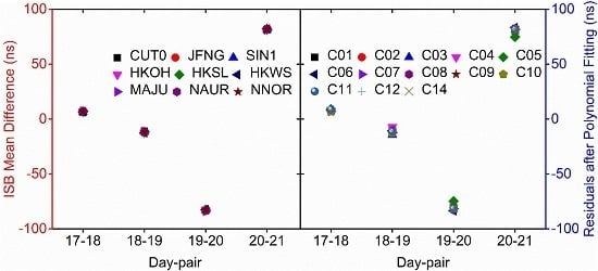
For further revelation of the linear dependency between satellite clock offsets and ISB, numerical verification was carried out. The test period for numerical verification was from 17 August to 21 August, which means that the experiments were carried out on the four day-pairs: August 17/18, 18/19, 19/20, and 20/21, 2015. Residual of the satellite clock offsets in a day-pair was calculated by making the difference between (predicted satellite clock from the polynomial fitting on basis of the satellite clocks from the last ten epochs on 1st day) and , which is the real satellite clock in the 1st epoch of 2nd day. The whole process is summarized as:
where denotes polynomial fitting using the satellite clock offsets from the last 10 epochs in the 1st day. By the extrapolation of , is derived. is the 1st epoch on the 2nd day. ISB difference between adjacent days is derived by:
The daily mean ISB value is indicated as . ISB value is expressed by with epoch number ranging from to . The subscript of a day-pair is expressed by and . ISB difference between the 1st and 2nd day is denoted as .
Figure 4 shows the ISB differences along with the satellite clock offset residuals in the four day-pairs. It is shown that ISB differences in these nine stations express different magnitudes in different day-pairs. In day-pairs 19/20 and 20/21, the most noticeable changes appear. It indicates that a large jump of satellite clock offsets occurred on 20 August, 2015. We checked the description comments on the reference clock in the header of the GBM product file, and concluded that the large jump is ascribed to the reference clock switch in the GBM precise clock product. The level of ISB differences in the nine stations is close in every day-pair. In addition, like the ISB difference, satellite clock offsets express the same phenomenon, which is for all satellites, the level of clock offsets residual is also close in each day-pair.
ISB differences among the nine stations and their statistics are illustrated in Table 4. At the same time, Table 5 includes satellite clock offset residuals and their statistics. Table 5 also includes some blank entries, which are due to the DI of the satellite clock in the adjacent days. Comparing Table 4 and Table 5, it is noticed that among all the four day-pairs, ISB differences at every station are correlated with the residuals of the satellite clock in all satellites. We can also see that if the satellite clock offset jumps take place, at the same time ISB jumps will appear. In the next part, we will make an analysis of the corresponding correlation coefficients.
Correlation coefficients were implemented as indicators of the correlation degree between two parameters. The correlation coefficients between the residuals of satellite clock offset in every satellite and ISB differences in every station were calculated from Table 4 and Table 5, and the results of correlation coefficients are shown in Table 6. Correlation analysis was only carried out using the satellites with residual data. It can be found from Table 6 that there is a strong positive correlation between every pair of the residual of satellite clock offset and ISB difference, since all the correlation coefficients are close to 1. In accordance with these findings, the incentive of satellite clock preprocessing becomes patently clear, which is to improve ISB continuity. In the next sections, we will present a detailed preprocessing process on the satellite clock to enhance ISB continuity.
3. Results and Discussion
In this section, a preprocessing method on the precise satellite products is proposed. First, the satellite clock product is converted from time domain into frequency domain, since it is more sensitive to the detection of ISB jumps. Then, extrema in the frequency domain clock data are detected and classified. After that, clock preprocessing is made to get a new preprocessed satellite clock product. At last, a test on the ISB continuity improvement is carried out after getting re-estimated ISB using processed satellite clock products.
3.1. Conversion from Time Domain into Frequency Domain
Larger clock jumps caused by considerable PMs can be easily detected in the time domain of the satellite clock in Figure 3. But as said before, the ISB continuity will not be destroyed by this type of clock jump. Thus, the true reason causing the ISB discontinuity needs to be found out. In addition, some smaller clock jumps can take place due to reference clock substitutions, weak PMs, clock day boundaries, which can be drowned in the large-scale satellite clock offset series. In order to overcome the above problems, the satellite clock is converted into the frequency domain from the time domain, since clock jumps, specifically small clock jumps, can be detected more sensitively by the satellite clock in the frequency domain.
Firstly, clock offset time series, excluding DIs as well as numerous PM epochs, are converted into CFD (clock frequency data). Fractional frequency data can be derived by taking the first differences of the phase data and dividing by the sampling interval , so it can be expressed as [23]:
Clock offset in the time domain in two adjacent epochs is expressed by and . Interval is set to five minutes. In the frequency domain, clock data is denoted as .
CFD series in August 2015 are shown in Figure 5. From Figure 5, we can see that the CFD series of every satellite has two extrema in epochs 5760 and 5472, the corresponding epoch date is the start time on 20 and 21 August, 2015. They are synchronous with the occurrence times of the most remarkable ISB gaps. Therefore, the true reason for those ISB jumps is the extrema in the CFD. It can be also noted that ISB continuity can be destroyed by other smaller extrema in the CFD as well. In another scope, it can be said that the most significant residuals of clock offset are indicated by the CFD extrema, and ISB differences between two adjacent epochs are considered as those ISB jumps. They have a great correlation. This finding deeply provides evidence of a strong correlation of the residuals of satellite clock offset with ISB differences.
3.2. Detection of Small Extrema in CFD
The median value is better able to reveal the characteristics of most data than the mean value. The median value more effectively avoids the impact of outliers. CFD extrema detection is more improved while applying the method of median filter-based robust estimation [24]. Small ISB jumps, which are not possible to observe directly from the CFD series, are detected by implementing this method. Following the median principle, the root mean square error of unit weight, marked with , is expressed as the normalized median for the absolute deviation between CFD and the median of CFD [25]. It is illustrated as:
CFD at epoch are indicated by . Median of is denoted by . The deviation between as well as is expressed as . The root mean square error of unit weight is expressed by . is considered as the threshold value. can be considered as an extremum of CFD if equation is satisfied. If not, is considered as a regular CFD point. An empirical model specifies the variability of . In this study, it is selected as 10, since we use the method of exhaustion with the value from 1 to 10 to check the result of extrema detection, and when the value is selected as 10, the performance of detection is best.
After the detections of CFD extrema, they will be classified by different causes. Depending on the types of CFD extrema, different preprocessing strategies on satellite clock products will be performed in the next section.
3.3. Classification of CFD Extrema and Clock Preprocessing
After the analysis, it is clear that clock jumps are caused by many reasons. For each of the reasons, the application of a different clock preprocessing strategy is necessary. These reasons are categorized after the detection of these CFD extrema. In the time domain, small PMs are the reasons for one kind of clock jump. They are not detected in the satellite clock offsets series. As PMs do not affect ISB continuity, preprocessing is not implemented for these types of extrema. The day boundaries of the clock caused by the daily solution strategy for the precise clock products result in the other kind of clock jump. The best solution to these types of extrema is to extend the estimation time period of satellite clock, e.g., one week or even one month. For these types of extrema, satellite clock offsets are not re-estimated in a long period in this discussion. Instead, two different strategies are implemented. Polynomial fitting using the previous data is utilized when the clock jump is over threshold value. We employ the clock data from the previous day as the essential data to fit a polynomial, then use this polynomial to predict the clock data for the next day. After that, the original satellite clock will be replaced with this predicted clock data to get a new clock product. If not, the original clock product is kept, as well as no processing implemented. The switch of the reference clock causes the last kind of clock jump. For these types of extrema, it is also solved by implementing the method of polynomial fitting.
Figure 6 illustrates the categorized types of extrema within CFD. We can see from Figure 6 that three different reasons mainly cause the extrema in CFD, which are: switches of the reference clock, clock day boundaries, and small PMs. When the reference clock is converted, extrema (jumps) will appear in each satellite. For these types of extrema, the magnitude is remarkable, so a method to generate a new satellite clock product by applying polynomial fitting is employed. In the current scenario of clock day boundaries, clock continuity will not be destroyed if the error is less than the threshold value, we apply no processing. Otherwise, the same polynomial fitting preprocessing procedure that is used for reference clock switches is utilized. The source of this threshold value is also from Equation (9), but in this part is selected as 3. In the case of the CFD extrema detection, the median filter is applied to detect the hidden smaller PMs in the time domain of satellite clock offsets. However, continuity of the estimated ISB is not affected by those small clock PMs, so we also make no processing.
A smooth and new clock product is gained once the preprocessing of satellite clock data is completed. After that, the ISB is re-estimated using the preprocessed satellite clock product, Figure 7 shows the new estimated ISB. Compared to the original ISB in Figure 2, the re-estimated ISB from this newly precise clock product has almost no jump, which is much more continuous and smoother.
3.4. Improvement of the ISB Continuity
For validating ISB continuity by applying the preprocessed satellite clock product, the statistical hypothesis technique is applied. The Equation (10) shows the statistics of the test (Zeng et al. 2017):
where represents the continuity factor. Variance on days and is denoted as and . The weighted ISB mean values on days and are and , which can be calculated from:
is the variance of ISB, and is the estimated ISB. The daily weighted mean value for ISB is expressed by .
Usually, means the critical value follows the normal distribution with the significance level . If the equation is satisfied, the ISB is discontinuous in two adjacent days, which means it varies greatly, or else ISB is continuous with no remarkable difference for two days. We can note that if the value of ISB continuity index is lower, the smoothness of ISB in two adjacent days is higher.
18 August and 20 August precise clock products were preprocessed previously in the above section. Thus, the test on 17–21 August was chosen here to analyze ISB continuity and its improvement. ISB series for HKSL, HKWS, HKOH, JFNG, SIN1, CUT0, NNOR, MAJU, and NAUR stations are illustrated in the top panel of Figure 8. Taking MAJU, CUT0 and HKOH stations as an example, their mean values and standard deviations are illustrated by the panel at the bottom. We can find from Figure 8 that on 18 and 20 August, the top panel shows the discontinuity of the ISB series. The mean of daily ISB values from the bottom panel further confirms this finding. Figure 9 shows the new ISB series after applying with the preprocessed precise clock products, along with the daily mean values. It is clear that the ISB discontinuity on 18 and 20 August was removed by the method of satellite clock preprocessing.
We designed two schemes to reveal the improvement of ISB continuity by the satellite clock preprocessing. In scheme a, the solution is using the original clock product. In scheme b, the results are applying with preprocessed clock products. The continuity factors for both schemes a and b are determined by Equation (10). The orange line in Figure 10 shows the calculated value of significant level 0.01 in normal distribution, which is 2.327.
ISB is regarded as continuous and stable in the adjacent days if the continuity factor is less than the critical value (2.327, the orange line). In scheme a, ISB in each adjacent day during the period of August 17–21 is discontinuous, as the continuity factor is all above the line of critical value. On the contrary, for scheme b, all the ISB continuity factors between adjacent days of August 17–21 are lower than the critical value, which means after satellite clock products are preprocessed, ISB continuity can be markedly improved. Table 7 includes the detailed statistics of the continuity factor. It is seen that, the same as in Figure 10, the ISB continuity can be significantly increased using scheme b. For day-pairs 17/18, 18/19, 19/20 and 20/21 August, the improvement rates are 62.4%, 79.5%, 99.6% and 99.0%. It can be concluded that it is possible to remarkably improve ISB continuity by applying preprocessing on precise satellite clock products.
4. Conclusions
In the time domain, large PMs as well as DIs in satellite clock products can be detected easily. However, it was found that PMs in satellite clock product were not the true cause for ISB jumps. Again, in the time domain, the linear correlation in satellite clock offsets and ISB was discussed. From the numerical results, a strong positive correlation was found between the residuals of satellite clock offset and ISB differences. Because of this, the method of making preprocessing on precise satellite clock products was proposed, which was used to remove the ISB discontinuity. Satellite clock data were converted from the time domain into the frequency domain. It made the detection of small jumps drowning in large-scale clock data much more sensitive. For detecting the clock jumps in the frequency domain data, a robust estimation method was applied, which was based on the median filter. After applying this method, we found that extrema in the data of the frequency domain were the real reason for ISB jumps. It was also found that clock day boundaries, reference clock switches, and small PMs were three individual reasons, which are categorized by the detection of smaller clock jumps. For all these three separate reasons, different strategies of clock preprocessing were implemented. After that, the re-estimation of ISB was performed using the preprocessed satellite clock product. From the ISB continuity improvement test, it was known that it was possible to improve the ISB continuity by 85.1% with the proposed preprocessing method on clock products. It showed the appropriateness of precise clock product preprocessing in terms of detecting and repairing the ISB jumps.
When we model ISB, ISB series need to be isolated into a number of components if the ISB series are discontinuous. But this problem can be overcome since we can apply the method of preprocessing on satellite clock products presented here. With this method, the smoother and continuous ISB series can be achieved. In that case, it is possible to obtain more sample points for modeling, as a result, the accuracy of modeling can also be enhanced. A future study on ISB modeling will be made using this method on the preprocessing of clock products.
Author Contributions
N.J. and Y.X. conceived and designed the study, made formal analysis, wrote the original draft; T.X. made some data analysis and visualization, and interpreted the results; G.X. and H.S. polished the manuscript. All authors have read and agreed to the published version of the manuscript.
Funding
This work is funded by National Key Research Program of China “Collaborative Precision Positioning Project” (2016YFB0501900), State Key Laboratory of Geo-Information Engineering, China (SKLGIE2017-Z-2-2), National Natural Science Foundation of China (41874032 and 41731069).
Conflicts of Interest
The authors declare no conflict of interest.
References
- Montenbruck, O.; Steigenberger, P.; Prange, L.; Deng, Z.; Zhao, Q.; Perosanz, F.; Romero, I.; Noll, C.; Stürze, A.; Weber, G.; et al. The Multi-GNSS Experiment (MGEX) of the International GNSS Service (IGS)–Achievements, prospects and challenges. Adv. Space Res. 2017, 59, 1671–1697. [Google Scholar] [CrossRef]
- Gu, S.; Lou, Y.; Shi, C.; Liu, J. BeiDou phase bias estimation and its application in precise point positioning with triple-frequency observable. J. Geod. 2015, 89, 979–992. [Google Scholar] [CrossRef]
- Odolinski, R.; Teunissen PJ, G.; Odijk, D. Combined BDS, Galileo, QZSS and GPS single-frequency RTK. GPS Solut. 2015, 19, 151–163. [Google Scholar] [CrossRef]
- Chen, J.; Wang, J.; Zhang, Y.; Yang, S.; Chen, Q.; Gong, X. Modeling and Assessment of GPS/BDS Combined Precise Point Positioning. Sensors 2016, 16, 1151. [Google Scholar] [CrossRef] [PubMed] [Green Version]
- Lou, Y.; Zheng, F.; Gu, S.; Wang, C.; Guo, H.; Feng, Y. Multi-GNSS precise point positioning with raw single-frequency and dual-frequency measurement models. GPS Solut. 2016, 20, 849–862. [Google Scholar] [CrossRef]
- Choy, S.; Bisnath, S.; Rizos, C. Uncovering common misconceptions in GNSS Precise Point Positioning and its future prospect. GPS Solut. 2017, 21, 13–22. [Google Scholar] [CrossRef]
- Li, X.; Zhang, X.; Ren, X.; Fritsche, M.; Wickert, J.; Schuh, H. Precise positioning with current multi-constellation Global Navigation Satellite Systems: GPS, GLONASS, Galileo and BeiDou. Sci. Rep. 2015, 5, 8328. [Google Scholar] [CrossRef] [PubMed]
- Torre, A.D.; Caporali, A. An analysis of intersystem biases for multi-GNSS positioning. GPS Solut. 2015, 19, 297–307. [Google Scholar] [CrossRef]
- Montenbruck, O.; Hauschild, A.; Hessels, U. Characterization of GPS/GIOVE sensor stations in the CONGO network. GPS Solut. 2011, 15, 193–205. [Google Scholar] [CrossRef]
- Tegedor, J.; Øvstedal, O.; Vigen, E. Precise orbit determination and point positioning using GPS, Glonass, Galileo and BeiDou. J. Geod. Sci. 2014, 4, 65–73. [Google Scholar] [CrossRef] [Green Version]
- Paziewski, J.; Wielgosz, P. Accounting for Galileo–GPS inter-system biases in precise satellite positioning. J. Geod. 2015, 89, 81–93. [Google Scholar] [CrossRef] [Green Version]
- Zhang, B.; Teunissen PJ, G.; Yuan, Y. On the short-term temporal variations of GNSS receiver differential phase biases. J. Geod. 2017, 91, 563–572. [Google Scholar] [CrossRef] [Green Version]
- Jiang, N.; Xu, Y.; Xu, T.; Xu, G.; Sun, Z.; Schuh, H. GPS/BDS short-term ISB modelling and prediction. GPS Solut. 2017, 21, 163–175. [Google Scholar] [CrossRef] [Green Version]
- Zeng, A.; Yang, Y.; Ming, F.; Jing, Y. BDS–GPS inter-system bias of code observation and its preliminary analysis. GPS Solut. 2017, 21, 1573–1581. [Google Scholar] [CrossRef]
- Jiang, N.; Xu, T.; Xu, Y.; Xu, G.; Schuh, H. Assessment of Different Stochastic Models for Inter-System Bias between GPS and BDS. Remote Sens. 2019, 11, 989. [Google Scholar] [CrossRef] [Green Version]
- Yang, Y.; Li, J.; Wang, A.; Xu, J.; He, H.; Guo, H.; Shen, J.; Dai, X. Preliminary assessment of the navigation and positioning performance of BeiDou regional navigation satellite system. Sci. China Earth Sci. 2014, 57, 144–152. [Google Scholar] [CrossRef]
- Zumberge, J.F.; Heflin, M.B.; Jefferson, D.C.; Watkins, M.M.; Webb, F.H. Precise point positioning for the efficient and robust analysis of GPS data from large networks. J. Geophys. Res. 1997, 102, 5005–5017. [Google Scholar] [CrossRef] [Green Version]
- Dach, R.; Schaer, S.; Lutz, S.; Meindl, M.; Beutler, G. Combining the Observations from Different GNSS. Agu. Fall Meet. Abstr. 2010, 12, 1–10. [Google Scholar]
- Geng, J.; Meng, X.; Dodson, A.H.; Teferle, F.N. Integer ambiguity resolution in precise point positioning: Method comparison. J. Geod. 2010, 84, 569–581. [Google Scholar] [CrossRef] [Green Version]
- Defraigne, P.; Bruyninx, C. On the link between GPS pseudorange noise and day-boundary discontinuities in geodetic time transfer solutions. GPS Solut. 2007, 11, 239–249. [Google Scholar] [CrossRef]
- Ge, M.; Gendt, G.; Rothacher, M.; Shi, C.; Liu, J. Resolution of GPS carrier-phase ambiguities in Precise Point Positioning (PPP) with daily observations. J. Geod. 2008, 82, 389–399. [Google Scholar] [CrossRef]
- Zhou, F.; Dong, D.; Li, P.; Li, X.; Schuh, H. Influence of stochastic modeling for inter-system biases on multi-GNSS undifferenced and uncombined precise point positioning. GPS Solut. 2019, 23, 59. [Google Scholar] [CrossRef]
- US Department of Commerce; NIST. Handbook of Frequency Stability Analysis; NIST: Gaithersburg, MD, USA, 2007; Volume 1065, pp. 1–123.
- Yang, Y.; He, H.; Xu, G. Adaptively robust filtering for kinematic geodetic positioning. J. Geod. 2001, 75, 109–116. [Google Scholar] [CrossRef]
- Huang, G.; Zhang, Q.; Li, H.; Fu, W. Quality variation of GPS satellite clocks on-orbit using IGS clock products. Adv. Space Res. 2013, 51, 978–987. [Google Scholar] [CrossRef]
Figure 1.
Geographic distribution of nine BeiDou navigation satellite system/global positioning system (BDS/GPS) stations. Three stations are marked red, which are Trimble receivers. Another three stations are marked blue, which are stations that have Leica receivers installed. The last three stations are marked green, which are SEPT receivers.

Figure 2.
Estimated ISBs at HKSL, HKWS, HKOH, JFNG, SIN1, CUT0, NNOR, MAJU, and NAUR stations. The squares pertain to Trimble receivers, the circles to Leica receivers, and the triangles to SEPT ones. The enlarged subfigure is the ISB gaps.
Figure 2.
Estimated ISBs at HKSL, HKWS, HKOH, JFNG, SIN1, CUT0, NNOR, MAJU, and NAUR stations. The squares pertain to Trimble receivers, the circles to Leica receivers, and the triangles to SEPT ones. The enlarged subfigure is the ISB gaps.

Figure 3.
Satellite clock offsets for the BDS system in the time domain through August 2015 with an interval of 5 min.
Figure 3.
Satellite clock offsets for the BDS system in the time domain through August 2015 with an interval of 5 min.

Figure 4.
The residuals of satellite clock and ISB differences in four day-pairs: August 17/18, 18/19, 19/20, and 20/21, 2015. The left panel is ISB differences, and the right panel shows satellite clock offset residuals.
Figure 4.
The residuals of satellite clock and ISB differences in four day-pairs: August 17/18, 18/19, 19/20, and 20/21, 2015. The left panel is ISB differences, and the right panel shows satellite clock offset residuals.

Figure 5.
BDS satellite clock in the frequency domain during August 2015.

Figure 6.
Clock functional data (CFD) extrema caused by three different reasons during August 2015. The causes, namely, clock day boundaries, switches of reference clocks, and small PMs, are displayed with various colors and symbols.
Figure 6.
Clock functional data (CFD) extrema caused by three different reasons during August 2015. The causes, namely, clock day boundaries, switches of reference clocks, and small PMs, are displayed with various colors and symbols.

Figure 7.
Re-estimated ISB series using preprocessed satellite clock products in HKSL, HKWS, HKOH, JFNG, SIN1, CUT0, NNOR, MAJU, and NAUR stations.
Figure 7.
Re-estimated ISB series using preprocessed satellite clock products in HKSL, HKWS, HKOH, JFNG, SIN1, CUT0, NNOR, MAJU, and NAUR stations.

Figure 8.
The mean values along with their standard deviations of original ISB series. The top panel displays original ISB series in all nine stations during 17–21 August. The mean values, standard deviations in MAJU, CUT0, and HKOH stations are illustrated in the bottom panel.
Figure 8.
The mean values along with their standard deviations of original ISB series. The top panel displays original ISB series in all nine stations during 17–21 August. The mean values, standard deviations in MAJU, CUT0, and HKOH stations are illustrated in the bottom panel.

Figure 9.
The mean values and their standard deviations for the new ISB series after the preprocessing of precise clock products in the top panel. The bottom panel shows mean values and standard deviations in MAJU, CUT0, and HKOH stations during 17–21 August.
Figure 9.
The mean values and their standard deviations for the new ISB series after the preprocessing of precise clock products in the top panel. The bottom panel shows mean values and standard deviations in MAJU, CUT0, and HKOH stations during 17–21 August.

Figure 10.
The values of the continuity factor for the two designed schemes (a, b). Three different signs are used to express MAJU, CUT0, and HKOH stations. The critical value for normal distribution with the significant value of 0.01 is expressed by the orange line.
Figure 10.
The values of the continuity factor for the two designed schemes (a, b). Three different signs are used to express MAJU, CUT0, and HKOH stations. The critical value for normal distribution with the significant value of 0.01 is expressed by the orange line.


Table 1.
Nine stations and their distributions, station names, receiver types, and firmware visions.
Table 1.
Nine stations and their distributions, station names, receiver types, and firmware visions.
| Station Name | Receiver Types and Firmware Ver. | Distributions |
|---|---|---|
| HKSL | Leica GRX1200 + GNSS/6.404 | 22.372N, 113.928E |
| HKWS | Leica GRX1200 + GNSS/6.404 | 22.434N, 114.335E |
| HKOH | Leica GRX1200 + GNSS/6.404 | 22.248N, 114.229E |
| JFNG | Trimble NeTR9/5.01 | 30.516N, 114.491E |
| SIN1 | Trimble NeTR9/5.01 | 1.343N, 103.679E |
| CUT0 | Trimble NeTR9/5.03 | 32.004S, 115.895E |
| NNOR | SEPT PolaRx4/2.9.0 | 31.049S, 116.193E |
| MAJU | SEPT PolaRx4TR/2.9.0Patch1 | 7.119N, 171.365E |
| NAUR | SEPT PolaRx4TR/2.9.0Patch1 | 0.552S, 166.926E |
Table 2.
Data processing strategies and observation models in BDS/GPS combined PPP.
| Items | Processing Strategies |
|---|---|
| Data | GPS + BDS in nine stations |
| Observations | Ionospheric-free linear combined phase and pseudorange data |
| Estimator | Extended Kalman filter (EKF) |
| Signal selection | BDS: B1/B2; GPS: L1/L2 |
| Interval rate | 30 s |
| Cut-off angle | 7° |
| Satellite orbit and clock | Fixed to GFZ MGEX (GBM) products |
| Zenith tropospheric delay/Mapping function | Zenith hydrostatic delay with Saastamoinen model, Zenith wet delay using random walk process with a constraint of 1 cm2/h; Global mapping function (GMF) is implemented as the mapping function |
| Ionospheric delay | The first-order error eliminated by the way of the ionospheric-free linear combination |
| Receiver phase center | In GPS, igs14.atx are used for phase center offset (PCO) and phase center variations (PCV) correction; In BDS, corrections are applied the same as GPS |
| Satellite phase center | igs14.atx are used for PCO and PCV correction |
| Windup effect | Corrected |
| Tidal effects | Corrected for solid tides, ocean loading, polar tides |
| Receiver clock | GPS receiver clock estimated as white noise |
| Inter-system bias (ISB) | Estimated as a piece-wise constant every 5 min (288 epochs one day) |
| Phase ambiguities | Estimated as constant in each arc |
Table 3.
The time of data interruption (DI) and phase modulation (PM) in the BDS satellite clock during August 2015. For brevity, the days of August are listed without the identification of the month. Satellites C08, C09, C10, and C14 are not listed here as they do not have any DI or PM.
Table 3.
The time of data interruption (DI) and phase modulation (PM) in the BDS satellite clock during August 2015. For brevity, the days of August are listed without the identification of the month. Satellites C08, C09, C10, and C14 are not listed here as they do not have any DI or PM.
| Satellite ID | Data Interruption (DI) Periods | Phase Modulation (PM) Points in the Time Domain | ||
|---|---|---|---|---|
| Periods | Corresponding Time (Day/Time in Aug. 2015) | Epoch | Corresponding Time (Day/Time in Aug. 2015) | |
| C01 | 3745–4032 | 14/00:00–14/23:55 | 5285 | 19/08:20 |
| 5185–5284 | 19/00:00–19/08:15 | |||
| C02 | 2176–2304 | 8/13:15–8/23:55 | 2305 | 9/00:00 |
| 3740–3745 | 13/23:35–14/00:00 | 3746 | 14/00:05 | |
| 5037–5472 | 18/11:40–19/23:55 | 5473 | 20/00:00 | |
| C03 | 865–1440 | 4/00:00–5/23:55 | 1441 2057 4932 5798 6718 | 6/00:00 8/03:20 18/02:55 21/03:05 24/07:45 |
| 2017–2056 | 8/00:00–8/03:15 | |||
| 4800–4931 | 17/15:55–18/02:50 | |||
| 5761–5797 | 21/00:00–21/03:00 | |||
| 6625–6717 | 24/00:00–24/07:40 | |||
| 8498–8928 | 30/12:05–31/23:55 | |||
| C04 | 4850–4896 | 17/20:05–17/23:55 | 4897 | 18/00:00 |
| 5761–5790 | 21/00:00–21/02:25 | 5791 | 21/02:30 | |
| C05 | 575–578 | 2/23:50–3/00:05 | 579 5185 6049 6774 | 3/00:10 19/00:00 22/00:00 24/12:25 |
| 2050–2054 | 8/02:45–8/03:05 | |||
| 2881–3168 | 11/00:00–11/23:55 | |||
| 5133–5184 | 18/19:40–18/23:55 | |||
| 5962–6048 | 21/16:45–21/23:55 | |||
| 6765–6773 | 24/11:40–24/12:20 | |||
| 8415–8425 | 30/05:10–30/06:00 | |||
| C06 | 577–653 | 3/00:00–3/06:20 | 654 | 3/06:25 |
| C07 | 7385–7396 | 26/15:20–26/16:15 | 7397 | 26/16:20 |
| C11 | 4765–4771 | 17/13:00–17/13:30 | 4772 6138 | 17/13:35 22/07:25 |
| 5074–5078 | 18/14:45–18/15:05 | |||
| 5206–5210 | 19/01:45–19/02:05 | |||
| 6049–6137 | 22/00:00–22/07:20 | |||
| 6442–6447 | 23/08:45–23/09:10 | |||
| C12 | 4897–4900 | 18/00:00–18/00:15 | 5185 | 19/00:00 |
| 5047–5184 | 18/12:30–18/23:55 | |||
Table 4.
ISB differences at nine stations in the day-pairs of August 17/18, 18/19, 19/20, and 20/21, 2015; unit: ns.
Table 4.
ISB differences at nine stations in the day-pairs of August 17/18, 18/19, 19/20, and 20/21, 2015; unit: ns.
| Day-Pairs | HKSL | HKWS | HKOH | JFNG | SIN1 | CUT0 | NNOR | MAJU | NAUR |
|---|---|---|---|---|---|---|---|---|---|
| 17–18 | 6.58 | 6.75 | 6.81 | 6.85 | 6.67 | 6.34 | 6.98 | 7.29 | 7.49 |
| 18–19 | −12.12 | −12.34 | −12.09 | −12.20 | −11.81 | −10.88 | −11.64 | −11.24 | −11.68 |
| 19–20 | −82.52 | −82.42 | −82.66 | −82.80 | −82.72 | −83.09 | −82.81 | −83.89 | −83.43 |
| 20–21 | 81.90 | 82.09 | 81.61 | 82.25 | 82.06 | 81.47 | 81.84 | 81.33 | 81.66 |
Table 5.
The residuals of satellite clock offset in the day-pairs of August 17/18, 18/19, 19/20, and 20/21, 2015 in BDS system; unit: ns.
Table 5.
The residuals of satellite clock offset in the day-pairs of August 17/18, 18/19, 19/20, and 20/21, 2015 in BDS system; unit: ns.
| Day-Pairs | C01 | C02 | C03 | C04 | C05 | C06 | |
| 17–18 | 7.37 | 9.02 | 7.92 | ||||
| 18–19 | −14.48 | −7.17 | −10.69 | ||||
| 19–20 | −80.95 | −79.38 | −74.81 | −83.41 | |||
| 20–21 | 80.95 | 79.38 | 74.81 | 83.41 | |||
| Day-Pairs | C07 | C08 | C09 | C10 | C11 | C12 | C14 |
| 17–18 | 7.03 | 7.83 | 6.36 | 6.97 | 8.65 | 7.40 | |
| 18–19 | −12.45 | −10.56 | −12.30 | −12.85 | −11.41 | −11.23 | |
| 19–20 | −81.66 | −82.61 | −81.46 | −81.68 | −81.47 | −81.98 | −81.15 |
| 20–21 | 81.66 | 82.61 | 81.46 | 81.68 | 81.47 | 81.98 | 81.15 |
Table 6.
The given value is 1-ρ, and ρ means the correlation coefficient between the residuals of satellite clock offset and ISB differences. So the smaller the given value, the closer the coefficient is to 1; unit: 10−5.
Table 6.
The given value is 1-ρ, and ρ means the correlation coefficient between the residuals of satellite clock offset and ISB differences. So the smaller the given value, the closer the coefficient is to 1; unit: 10−5.
| Correlation Coefficients | C06 | C07 | C08 | C09 | C10 | C11 | Mean |
|---|---|---|---|---|---|---|---|
| HKSL | −5 | −2 | −5 | −1 | −4 | −8 | −4 |
| HKWS | −7 | −1 | −7 | −1 | −2 | −8 | −4 |
| HKOH | −3 | −2 | −3 | −3 | −4 | −5 | −3 |
| JFNG | −5 | −1 | −5 | −1 | −3 | −7 | −4 |
| SIN1 | −3 | −3 | −3 | −2 | −6 | −8 | −4 |
| CUT0 | −2 | −16 | −2 | −13 | −22 | −17 | −12 |
| NNOR | −1 | −5 | −1 | −5 | −8 | −6 | −4 |
| MAJU | −2 | −18 | −2 | −20 | −23 | −8 | −12 |
| NAUR | −1 | −9 | −1 | −12 | −12 | −2 | −6 |
Table 7.
ISB continuity factors among four different day-pairs August 17/18, 18/19, 19/20 and 20/21. Scheme a is the ISB continuity factor from the original clock, and scheme b is the ISB continuity with the preprocessed clock.
Table 7.
ISB continuity factors among four different day-pairs August 17/18, 18/19, 19/20 and 20/21. Scheme a is the ISB continuity factor from the original clock, and scheme b is the ISB continuity with the preprocessed clock.
| Day-Pairs | 17/18 | 18/19 | 19/20 | 20/21 | ||||
|---|---|---|---|---|---|---|---|---|
| Station ID | a | b | a | b | a | b | a | b |
| HKSL | 2.55 | 1.09 | 4.69 | 1.07 | 37.39 | 0.03 | 36.46 | 0.28 |
| HKWS | 2.57 | 1.07 | 4.74 | 1.08 | 4.74 | 0.08 | 37.22 | 0.22 |
| HKOH | 3.12 | 1.22 | 5.41 | 1.18 | 41.00 | 0.01 | 39.04 | 0.44 |
| JFNG | 2.82 | 1.15 | 4.55 | 0.96 | 33.29 | 0.12 | 37.50 | 0.10 |
| SIN1 | 2.86 | 1.15 | 4.77 | 0.99 | 32.22 | 0.09 | 34.37 | 0.36 |
| CUT0 | 1.70 | 0.66 | 2.93 | 0.56 | 22.21 | 0.05 | 22.59 | 0.43 |
| NNOR | 2.52 | 0.88 | 4.08 | 0.78 | 28.41 | 0.15 | 28.41 | 0.43 |
| MAJU | 2.02 | 0.56 | 3.56 | 0.62 | 26.10 | 0.34 | 26.10 | 0.31 |
| NAUR | 2.16 | 0.63 | 3.73 | 0.64 | 25.77 | 0.13 | 25.24 | 0.32 |
| Mean | 2.48 | 0.93 | 4.27 | 0.88 | 27.90 | 0.11 | 31.88 | 0.32 |
| Improvement rate | 62.4% | 79.5% | 99.6% | 99.0% | ||||
© 2020 by the authors. Licensee MDPI, Basel, Switzerland. This article is an open access article distributed under the terms and conditions of the Creative Commons Attribution (CC BY) license (http://creativecommons.org/licenses/by/4.0/).
Share and Cite
MDPI and ACS Style
Jiang, N.; Xu, T.; Xu, Y.; Xu, G.; Schuh, H. Detecting and Repairing Inter-system Bias Jumps with Satellite Clock Preprocessing. Remote Sens. 2020, 12, 850. https://0-doi-org.brum.beds.ac.uk/10.3390/rs12050850
AMA Style
Jiang N, Xu T, Xu Y, Xu G, Schuh H. Detecting and Repairing Inter-system Bias Jumps with Satellite Clock Preprocessing. Remote Sensing. 2020; 12(5):850. https://0-doi-org.brum.beds.ac.uk/10.3390/rs12050850
Chicago/Turabian StyleJiang, Nan, Tianhe Xu, Yan Xu, Guochang Xu, and Harald Schuh. 2020. "Detecting and Repairing Inter-system Bias Jumps with Satellite Clock Preprocessing" Remote Sensing 12, no. 5: 850. https://0-doi-org.brum.beds.ac.uk/10.3390/rs12050850
Note that from the first issue of 2016, this journal uses article numbers instead of page numbers. See further details here.