Landsat 8 Virtual Orange Band for Mapping Cyanobacterial Blooms


Center for Geospatial Research, Department of Geography, University of Georgia, Athens, GA 30602, USA
*
Author to whom correspondence should be addressed.
Remote Sens. 2020, 12(5), 868; https://0-doi-org.brum.beds.ac.uk/10.3390/rs12050868
Submission received: 10 February 2020
/
Revised: 28 February 2020
/
Accepted: 5 March 2020
/
Published: 8 March 2020
(This article belongs to the Section Remote Sensing Communications)
Abstract
:The Landsat 8 Operational Land Imager (OLI) has a panchromatic band (503–676 nm) that can be used to derive a novel virtual orange band (590–635 nm) by using the multispectral green band and red band components. The orange band is useful for the accurate detection and quantification of phycocyanin (PC), an accessory pigment in toxin-producing cyanobacterial blooms, because of the specific light absorption characteristics of PC around 600–625 nm. In this study, we compared the Landsat 8 OLI’s and Sentinel-3 Ocean and Land Color Instrument’s (OLCI) derived orange band reflectance and PC products corresponding to a same-date overpass during a severe cyanobacterial bloom in Lake Erie, USA. The goal was to determine if the OLI’s virtual orange band can produce results equivalent to the OLCI’s actual orange band. Band-by-band match-ups used the OLI’s top-of-atmosphere (TOA) reflectance versus TOA reflectance from the OLCI, and surface reflectance (SR) from the OLI versus SR from the OLCI. A significant correlation was observed between the OLI’s and OLCI’s derived orange band TOA reflectance (R2 = 0.86; p < 0.001; NRMSE = 9.01%) and orange band SR (R2 = 0.93; p < 0.001; NRMSE = 20.23%). The PC map produced using the best-fit empirical models from both sensors showed similar PC spatial patterns and concentration levels in the western basin of Lake Erie. The results from this research are particularly important for the study of smaller inland waterbodies with the 30 m resolution of the OLI, which cannot be studied with the 300 m resolution of OLCI data, and for analyzing historical bloom events before the launch of the OLCI. Although more analysis and validation need to be conducted, this study opens up Landsat 8’s applicability in research on cyanobacterial harmful algal blooms (cyanoHABs).
Keywords:
cyanobacteria; phycocyanin; cyanoHABs; Lake Erie; Landsat 8 OLI; orange band; Sentinel 3-OLCI
1. Introduction
Cyanobacterial harmful algal blooms (cyanoHABs) have become a major concern for water resource managers, environmental agencies, and public health organizations across the globe because they pose serious health problems to humans and livestock via cyanotoxin production and result in significant negative economic impacts ($2.2 billion annually in the U.S. alone) [1,2]. CyanoHABs are comprised of photosynthesizing prokaryotic cyanobacteria that multiply rapidly in favorable environmental conditions to form harmful mats or blooms. Early detection and monitoring of cyanoHABs is critical for developing management strategies in advance, limiting their environmental exposure, and reducing the associated economic and health impacts. Many past studies have used phycocyanin (PC), an accessory pigment in cyanobacteria, as a proxy for the detection and monitoring of cyanoHABs, using their specific absorption feature around 600–625 nm in remotely sensed reflectance data [3,4,5]. Various remote sensing platforms, sensors, and techniques such as optical buoys, hyperspectral drones, and airborne and spaceborne sensors can use the 620 nm band to detect and quantify PC concentrations. However, only one operational satellite sensor from the European Space Agency (ESA), that is, the Sentinel-3 Ocean and Land Color Instrument (OLCI), has the 620 nm band, and none of the NASA operational satellite sensors do. Therefore, cyanoHAB detection and monitoring using satellite sensors is currently limited to large inland waterbodies with the coarse spatial resolution (300 m) of the OLCI and this, too, has been limited since its launch in 2016.
To overcome the above limitations, Castagna et al. [5] recently proposed the use of the Landsat 8 Operational Land Imager (OLI) to create a virtual orange band (band center: 613 nm; bandwidth 590–635 nm) at a 30 m spatial resolution using the panchromatic (pan), green, and red bands. Though the pan band is typically used for enhancing the spatial resolution to create “sharpened” images, it also contains spectral information that can be used to isolate a unique orange spectral channel. While the results of that [5] study are promising, their approach relied solely on an in situ dataset and simulated OLI data. In a second study, Castagna et al. [6] used satellite data to validate the OLI’s virtual band with same-date OLCI data. However, their study did not show a comparison between the estimated PC maps derived from the new virtual orange band and PC maps using the OLCI’s actual orange band. Therefore, we framed this study to go beyond an individual band comparison between the two sensors and compared various band combinations that can be used to derive PC concentration maps using these sensors. Although Castagna et al. [5] originally inspired this study, we uniquely demonstrate that the OLI’s virtual orange band can be used to derive PC concentrations similar to the OLCI’s actual orange band.
We aim to validate the approach of Castagna et al. [5] by using the OLCI’s orange band as reference data in order to test the efficacy of the OLI’s virtual orange band in a variety of contexts. By analyzing the difference in reflectance values between the OLI and OLCI for a same-date image, we can estimate the virtual orange band’s performance and potential for filling the data gap posed by the OLCI sensor. If the OLI’s virtual orange band can be shown as an acceptable replacement or predictor for the OLCI’s orange band, the spatial coverage, frequency, and volume of data available for cyanoHAB detection will increase dramatically. The use of OLI data for PC estimation would be particularly useful for studies requiring data between 2013 (after the ESA’s Medium Resolution Imaging Spectrometer (MERIS) data collection stopped and the beginning of the OLI) and 2016 (start of OLCI data acquisition), and for cyanoHAB detection in small- to medium-sized inland waterbodies.
2. Materials and Methods
2.1. Derivation of the OLI’s Orange Band
The approach of Castagna et al. [5] used a diverse in situ dataset of water leaving reflectance collected over Dutch and Belgian lakes. To derive the orange band, they divided the spectral response function (SRF) of the pan band into four components (Figure 1a). They subtracted contributions from the green (Component II) and red (Component IV) channels from the pan band, and the contribution from Component I was compensated in the multiple linear regression coefficients to derive the orange band using Equation (1):
where ρw is water leaving reflectance and parentheses represent the standard deviation for individual coefficients.
ρw(orange) = 2.4120(±0.1143)ρw(pan) − 0.9738(±0.0503)ρw(green) − 0.2999(±0.0667)ρw(red)
The coefficients from Equation (1) were implemented in the open source software ACOLITE (https://odnature.naturalsciences.be/remsem/software-anddata/acolite) to derive the virtual orange band from the OLI data. ACOLITE uses the dark spectrum fitting (DSF) atmospheric correction method by Vanhellemont [7]. The DSF combined with the relative SRF of the pan band was used for the atmospheric correction of the OLI’s pan band in ACOLITE, and subsequently the orange band was derived using Equation (1).
2.2. Correlation between OLI and OLCI Bands
To recreate and validate the approach of Castagna et al. [5], we considered the OLCI sensor as the reference since it has an orange band centered at 620 nm. First, the coincident cloud-free OLI (16:10:27 Z) and OLCI (17:19:35 Z) L1 data (both overpasses were on 26 September 2017) for Lake Erie’s western basin were downloaded from USGS EarthExplorer (https://earthexplorer.usgs.gov/) and EUMETSAT’s Copernicus Online Data Access (CODA) website (https://coda.eumetsat.int/#/home). Next, the OLI data were atmospherically corrected using ACOLITE software, and the OLCI data were atmospherically corrected using the iCOR (https://remotesensing.vito.be/case/icor) plugin in SNAP software (https://step.esa.int/main/toolboxes/snap/). We used two different software platforms for the atmospheric correction because atmospheric correction of the pan band is currently not available in the USGS Landsat 8 L2 data or in any other software except ACOLITE, which is required to derive the virtual orange band using Equation (1), and ACOLITE is not designed to process the OLCI data. The OLI’s pixels were spatially re-sampled to 300 m × 300 m (using the nearest neighborhood algorithm), and re-projected onto the World Geodetic System’s (WGS) 1984 geographic coordinate system to match the OLCI pixels. Top-of-atmosphere (TOA) reflectance and surface reflectance (SR) for the blue, green, orange, and red bands corresponding to 300 random pixels (Figure 1b) over Lake Erie were compared between the OLI and OLCI using a least-square regression. The band-to-band difference was assessed using percentage normalized root mean square error (%NRMSE) considering the OLCI as the reference sensor using Equation (2). The slope derived from the TOA regression was compared with the SR regression slope to observe the effect of atmospheric correction differences between the different software platforms.
where yi is TOA or SR corresponding to the OLI for the ith pixel of a particular band, xi is TOA or SR corresponding to the OLCI for the ith pixel of a particular band, n is the total number of pixels of a particular band, and xmax and xmin are the maximum and minimum values of the TOA or SR corresponding to a particular band of the OLCI.
Note that we did not do any cross-calibration between the two sensors because of the lack of in-situ reflectance data coincident to the satellite imageries. Therefore, we do not know which sensor’s reflectance is more accurate post atmospheric correction, and errors reported here are just the difference between the two sensors and not the actual error estimates.
2.3. PC Estimation Using the OLI and OLCI
The in situ PC data for Lake Erie is publicly available on NOAA’s Great Lakes Environmental Research Laboratory (GLERL) website (https://www.glerl.noaa.gov/res/HABs_and_Hypoxia/habsMon.html). For PC concentration measurements, water samples filtered through 47 mm GF/F filters (Whatman, 47 mm) were submerged in a phosphate buffer (Ricca Chemical, pH 6.8) using two freeze–thaw cycles, followed by sonication [8]. The extracted solutions were run through a Turner Aquafluor fluorometer, and fluorescence values were converted to PC concentrations using a calibration curve obtained from a series of dilutions of a commercial standard (Sigma-Aldrich) [9]. The cloud-free OLI and OLCI data corresponding to sampling dates or nearby dates were matched up with in situ data to establish an empirical relationship for PC estimation. A total of 16 (n = 16) PC data were matched-up with the OLI and OLCI derived SR (averaged 3 × 3 pixel window) data from three dates (22 August 2016, 26 September 2017, and 05 August 2018) of satellite overpasses. We tested various empirical models with the orange band combination to derive consistent PC maps from both the OLI and OLCI data. The PC maps derived from both sensors were compared qualitatively and quantitatively. We also created PC maps for past cyanoHABs in Lake Erie using OLI data for a period when the OLCI was not launched and discussed the potential issues with the PC model and what further improvements are needed in deriving the virtual orange band or the PC model. The overall processing steps involved in this study are presented in Figure 2.
3. Results
3.1. OLI and OLCI TOA Reflectance
The linear regression between the OLI- and OLCI-derived TOA reflectance showed a significant correlation (R2 = 0.86–0.90; p < 0.001) for each visible band (Figure 3a–d). However, a significant underestimation was observed in the OLI’s blue band (480 nm) compared to the OLCI’s blue band (490 nm) (Figure 3a). The major factors responsible for the differences between the two sensors are the differences in the band-wise signal-to-noise ratio (SNR), band center locations, bandwidth, and magnitude of the spectral response function. The difference between the TOA reflectance from both sensors decreased gradually with increasing wavelength. The differences seem to be related to residual Rayleigh scattering, which affects the shorter wavelengths more strongly compared to the longer wavelengths. This was further supported by error estimates (%NRMSE), which showed the blue band to have the highest error (24.96%) and the red band to have the lowest error (8.84%) (Table 1). The more important finding in this process was the reasonable error range for the orange band (9.01%), which is the focus of this study.
3.2. OLI and OLCI Surface Reflectance
TOA reflectance contains up to only 10% of the signal received from the water surface [10]; therefore, we compared the SR for both sensors. The SR comparison between the OLCI and OLI bands revealed a significant correlation for all visible bands (R2 = 0.81 to 0.95) (Figure 3e–h). In addition, the regression slopes remained similar before and after the atmospheric correction for all bands, suggesting consistent atmospheric correction regardless of the type of software used for both sensors (Figure 3a–h). The green bands for both sensors have the same band center (560 nm) and showed the lowest error (6.07%) compared to the other three bands (Table 1). The red band with the highest band center difference (10 nm) produced the highest error (27.93%) (Table 1). In addition, it was expected that the 665 nm band would absorb more light in bloom conditions compared to the 655 nm band, and that is evidenced in Figure 3h. The orange band (613 nm) resulted in a 20% error compared to the OLCI’s 620 nm band (Table 1). The 613 nm band showed higher reflectance compared to the 620 nm band (Figure 3g), which was also expected because 620 nm absorbs more light (PC absorption feature) in intense cyanoHAB conditions. Note that the errors reported here are relative to the OLCI’s SR, which may have its own residual errors.
3.3. Correlation between the OLI’s and OLCI’s SR Band Combinations
We compared several indices derived using the band combination of these sensors. Usually, band ratio, spectral shape, and band subtractions are the most commonly used band combinations for developing empirical water quality models [11,12,13]. The blue/green band ratio showed a significant correlation (R2 = 0.93; p < 0.001) between the OLCI and OLI (Figure 4a). Past studies have used the blue/green band ratio for quantifying algae blooms. However, the orange band (~620 nm) is specific to cyanobacterial blooms because of PC absorption and less interference from other phytoplankton pigments [13,14,15]. Therefore, PC-based semi-empirical models incorporating the orange band were investigated. Comparison between the OLCI’s and OLI’s orange/red band ratio showed a lower correlation (R2 = 0.28), but it was still significant (p < 0.01) (Figure 4b). The large difference in R2 is mainly because of band center differences between the two sensors. The spectral shape model by Qi et al. [12] showed a significant correlation (R2 = 0.73; p < 0.001) (Figure 4c). In addition, the inverse of band differences between orange and red showed a significant correlation (R2 = 0.61; p < 0.001) (Figure 4d). These results suggest that common empirical models using both sensors can be utilized to produce similar products if calibrated with the same in situ data. This is an important finding, which addresses the temporal data gap constraint experienced by Landsat to effectively monitor these high-frequency environmental phenomena.
4. Discussion
4.1. PC Model Comparison Using the OLI and OLCI
All band combinations investigated in this study were compared using in situ PC data and corresponding SR derived from the OLI’s and OLCI’s pixels. The orange/red band ratio (613/655 nm) resulted in the best fit model for the OLI (R2 = 0.55; p < 0.001) (Table 2). Many past studies have successfully used the band ratio for PC estimation [11,14,15,16]. For example, [11] used the band ratio (650/625 nm) for PC estimation in Carter Lake, and [16] found a significant correlation (R2 = 0.66; p < 0.001) between in situ PC and the band ratio (625/650 nm) in the Baltic Sea. However, in our study, the OLCI’s orange/red ratio (620/665 nm) showed an insignificant (R2 = 0.16; p = 0.11) correlation (Table 2). This result suggests the importance of differences in the band center (OLI: 655 nm; OLCI: 665 nm) and bandwidth (OLI: 640–670 nm; OLCI: 660–670 nm) between the OLI’s and OLCI’s spectral architecture. On the other hand, the normalized difference of the orange (620 nm) and red-edge (709 nm) band resulted in a significant correlation (R2 = 0.74; p < 0.001) for the OLCI (Table 2). Although these results show promise for cross-sensor calibration for PC estimation, more samples (coincident match-up data) are needed for a robust satellite-based PC model and for independent validation in the future. Moreover, for cross-calibration, a common software platform should be used in the future for atmospheric correction of both sensors to minimize the potential source of uncertainty that might arise using two different software platforms, as in this study.
4.2. PC Maps Using the OLI and OLCI
To observe the similarities in spatial patterns and concentration range, the best-fit PC models corresponding to the OLI and OLCI were implemented on a same-date overpass (26 September 2017) dataset. PC maps derived from both sensors showed a similar spatial pattern and concentration range (Figure 5a–d). Both PC maps followed the same bloom pattern observed in the corresponding true color images, which suggests that the PC model effectively isolated the bloom area. One noticeable difference between the OLI- and OLCI-derived PC maps was observed in the northernmost part of Lake Erie (Figure 5c,d), where the OLI showed higher PC values. This is mainly because of the underestimation of the orange band reflectance in colored dissolved organic matter (CDOM)-dominated waters (dark blue color regions in the true color images; Figure 5a,b), where maximum absorption occurs in the blue band. There is an overlap between a narrow spectral region (500–510 nm) of the OLI’s pan band with the OLI’s blue band (Figure 1a), which was not accounted for in the derivation of the virtual orange band. This could have resulted in a slight underestimation of orange band reflectance. In contrast to the OLI’s PC map, the OLCI’s true-orange-band-derived PC map did not show higher PC values in the same northernmost part of the lake. Further, the orange/red band ratio-based PC model was implemented on OLI data before 2016, a period for which OLCI data are not available. The PC map successfully captured the bloom area corresponding to the true color images (Figure 6a–d). However, it was observed that it produced higher PC values for the sediment-dominated regions (Figure 6a,b). This is mainly because of the underestimation of the orange band compared to the red band in sediment-dominated regions, which resulted in lower orange-red band ratio values and overestimated PC concentrations. The underestimation of the orange band in sediment-dominated regions might have resulted from the higher reflectance signal in the green band and differences in the spectral response function between the panchromatic band and corresponding green channel (Figure 1a). Therefore, caution must be taken in utilizing the orange band derived from the OLI sensor in both CDOM- and sediment-dominated regions. Further improvements are needed to overcome this issue in the future with flexible coefficients in the empirical orange band model (Equation (1)) for different water types.
There is certainly more work to be done in this area to further validate the OLI’s orange band retrieval method and its effectiveness in estimating PC concentrations. This study is a prototype which validated the orange band output for only one geographic location; unique features of other water bodies may enhance or deteriorate the performance of the orange band retrieval method. Intensive validation of this method will open up a number of possibilities for utilizing Landsat data to generate new information using overlapping bands. The scope of this study is not limited to only the OLI sensor, but can be used for other sensors such as the Landsat 7-ETM+ which has a panchromatic band (520–900 nm) overlapping with green (520–600 nm), red (630–690 nm), and NIR bands (770–900 nm). Retrieval of the orange band from Landsat 7 (600–630 nm) and Landsat 8 (590–635 nm) could help in creating a long-term time series of cyanoHABs for inland waterbodies, and fill the time gap between the Envisat-Medium Resolution Imaging Spectrometer’s (MERIS) expiration (2012) and Sentinel-3 OLCI’s launch (2016). Moreover, the 30 m spatial resolution of a Landsat would provide an opportunity to capture the cyanoHABs in small waterbodies, which currently cannot be studied using the 300 m spatial resolution of OLCI data.
5. Conclusions
This study validated the approach of Castagna et al. [5] to derive the OLI’s virtual orange band and its potential for PC estimation. The OLI and OLCI orange bands showed a significant correlation (R2 = 0.93; p < 0.001), suggesting that the OLI can serve as a reliable alternative and proxy for the OLCI’s orange data. The semi-empirical band ratio and band-difference-based PC models corresponding to the OLI and OLCI effectively captured the spatial pattern and concentration of a cyanobacteria bloom in the western part of Lake Erie. However, sediment-dominated regions resulted in erroneous PC estimation, which needs to be fixed in future studies by incorporating various optical water types to derive flexible coefficients in simulation of the OLI’s orange band.
Author Contributions
A.K. processed and analyzed the data; A.K. wrote the manuscript; D.R.M. reviewed and edited the manuscript; N.I. helped in processing and writing the manuscript; D.R.M. provided supervision; A.K. produced the visualization. All authors have read and agreed to the published version of the manuscript.
Funding
Partial funding for this work was provided by the National Science Foundation (NSF) (Grant #CCF-1442672) under the CyanoTRACKER project.
Conflicts of Interest
The authors declare no conflict of interest.
References
- Li, L.; Li, L.; Song, K. Remote sensing of freshwater cyanobacteria: An extended IOP inversion model of inland waters (IIMIW) for partitioning absorption coefficient and estimating phycocyanin. Remote Sens. Environ. 2015, 157, 9–23. [Google Scholar] [CrossRef]
- Duan, H.; Ma, R.; Hu, C. Evaluation of remote sensing algorithms for cyanobacterial pigment retrievals during spring bloom formation in several lakes of East China. Remote Sens. Environ. 2012, 126, 126–135. [Google Scholar] [CrossRef]
- Hunter, P.D.; Tyler, A.N.; Carvalho, L.; Codd, G.A.; Maberly, S.C. Hyperspectral remote sensing of cyanobacterial pigments as indicators for cell populations and toxins in eutrophic lakes. Remote Sens. Environ. 2010, 114, 2705–2718. [Google Scholar] [CrossRef] [Green Version]
- Yan, Y.; Bao, Z.; Shao, J. Phycocyanin concentration retrieval in inland waters: A comparative review of the remote sensing techniques and algorithms. J. Gt. Lakes Res. 2018, 44, 748–755. [Google Scholar] [CrossRef]
- Castagna, A.; Simis, S.; Dierssen, H.; Vanhellemont, Q.; Sabbe, K.; Vyverman, W. Extending the operational land imager/landsat 8 for inland water research: Retrieval of an orange band from pan and ms bands. In Proceedings of the Ocean Optics Conference (Ocean Optics XXIV), Dubrovnik, Croatia, 7–12 October 2018; Available online: https://oceanopticsconference.org/extended/Castagna_Alexandre.pdf (accessed on 8 June 2019).
- Castagna, A.; Simis, S.; Dierssen, H.; Vanhellemont, Q.; Sabbe, K.; Vyverman, W. Validation of the Operational Land Imager orange contra-band retrieval for inland water quality applications. In Proceedings of the Living Planet Symposium, Milan, Italy, 13–17 May 2019; Available online: https://eo.belspo.be/sites/default/files/content/LPS19/13.pdf (accessed on 10 December 2019).
- Vanhellemont, Q. Adaptation of the dark spectrum fitting atmospheric correction for aquatic applications of the Landsat and Sentinel-2 archives. Remote Sens. Environ. 2019, 225, 175–192. [Google Scholar] [CrossRef]
- Horváth, H.; Kovacs, A.W.; Riddick, C.; Présing, M. Extraction methods for phycocyanin determination in freshwater filamentous cyanobacteria and their application in a shallow lake. Eur. J. Phycol. 2013, 48, 278–286. [Google Scholar] [CrossRef] [Green Version]
- Ogashawara, I. The use of Sentinel-3 Imagery to monitor cyanobacterial blooms. Environments 2019, 6, 60. [Google Scholar] [CrossRef] [Green Version]
- Gordon, H.R. Atmospheric correction of ocean color imagery in the Earth Observing System Era. J. Geophys. Res. 1997, 102, 17081–17106. [Google Scholar] [CrossRef]
- Schalles, J.; Yacobi, Y. Remote detection and seasonal patterns of phycocyanin, carotenoid and Chl-a pigments in eutrophic waters. Ergeb. Limnol. 2000, 55, 153–168. [Google Scholar]
- Qi, L.; Hu, C.; Duan, H.; Cannizzaro, J.; Ma, R. A novel MERIS algorithm to derive cyanobacterial phycocyaninpigment concentrations in a eutrophic lake: Theoretical basis and practical considerations. Remote Sens. Environment 2014, 154, 298–317. [Google Scholar]
- Mishra, S.; Mishra, D.R. A novel remote sensing algorithm to quantify phycocyanin in cyanobacterial algal blooms. Environ. Res. Lett. 2014, 9, 114003. [Google Scholar] [CrossRef]
- Simis, S.G.H.; Peters, S.W.M.; Gons, H.J. Remote sensing of the cyanobacterial pigment phycocyanin in turbid inland water. Limnol. Oceanogr. 2005, 50, 237–245. [Google Scholar] [CrossRef]
- Mishra, S.; Mishra, D.R.; Schluchter, W.M. A novel algorithm for predicting phycocyanin concentrations in cyanobacteria: A proximal hyperspectral remote sensing approach. Remote Sens. 2009, 1, 758–775. [Google Scholar] [CrossRef] [Green Version]
- Wozniak, M.; Bradtke, K.M.; Darecki, M.; Krężel, A. Empirical Model for Phycocyanin Concentration Estimation as an Indicator of Cyanobacterial Bloom in the Optically Complex Coastal Waters of the Baltic Sea. Remote Sens. 2016, 8, 212. [Google Scholar] [CrossRef] [Green Version]
Figure 1.
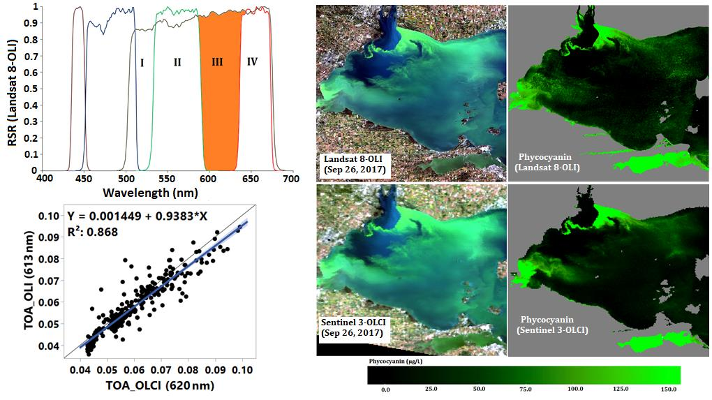
The Landsat 8 Operational Land Imager’s (OLI) relative spectral response (RSR) for visible wavelengths. (a) Castagna et al. [5] divided the RSR of the panchromatic band (503–676 nm) into four components (I, II, II, and IV), and Component III is the virtual orange band (590–635 nm). (b) The Landsat 8 OLI image (re-sampled to 300 m resolution) of the western basin of Lake Erie showing 300 random pixels used in deriving the virtual orange band.
Figure 1.
The Landsat 8 Operational Land Imager’s (OLI) relative spectral response (RSR) for visible wavelengths. (a) Castagna et al. [5] divided the RSR of the panchromatic band (503–676 nm) into four components (I, II, II, and IV), and Component III is the virtual orange band (590–635 nm). (b) The Landsat 8 OLI image (re-sampled to 300 m resolution) of the western basin of Lake Erie showing 300 random pixels used in deriving the virtual orange band.

Figure 2.
Overall schematic diagram of processing steps for Landsat 8 (LS8) OLI and Sentinel 3 (Sen3)-Ocean and Land Color Instrument (OLCI) data in this study. PC: phycocyanin; SR: surface reflectance; TOA: top-of-atmosphere.
Figure 2.
Overall schematic diagram of processing steps for Landsat 8 (LS8) OLI and Sentinel 3 (Sen3)-Ocean and Land Color Instrument (OLCI) data in this study. PC: phycocyanin; SR: surface reflectance; TOA: top-of-atmosphere.

Figure 3.
Regression between the OLCI- and OLI-derived TOA reflectance for the (a) blue, (b) green, (c) orange, and (d) red bands. Regression between the OLCI- and OLI-derived SR for the (e) blue, (f) green, (g) orange, and (h) red bands. Blue lines are trend lines and black lines are a 1:1 line for each band.

Figure 4.
Regression between the OLCI- and OLI-derived SR band ratio: (a) blue/green, (b) orange/red. (c) Spectral shape (SS) with orange band as the central wavelength; and (d) the band difference of the inverse of the orange and red bands.
Figure 4.
Regression between the OLCI- and OLI-derived SR band ratio: (a) blue/green, (b) orange/red. (c) Spectral shape (SS) with orange band as the central wavelength; and (d) the band difference of the inverse of the orange and red bands.

Figure 5.
(a) LS8-OLI and (b) Sen3-OLCI true color images from the same-date (26 September 2017) overpass during a cyanobacteria bloom in Lake Erie. The corresponding PC maps derived using (c) OLI and (d) OLCI data.
Figure 5.
(a) LS8-OLI and (b) Sen3-OLCI true color images from the same-date (26 September 2017) overpass during a cyanobacteria bloom in Lake Erie. The corresponding PC maps derived using (c) OLI and (d) OLCI data.

Figure 6.
LS8-OLI-derived PC maps corresponding to a cyanobacteria bloom in Lake Erie on (a,b) 10 October 2013 and (c,d) 27 September 2014. The turbid region (marked with a circle) showed lower values of the orange band compared to the red band and consequently higher PC estimation.
Figure 6.
LS8-OLI-derived PC maps corresponding to a cyanobacteria bloom in Lake Erie on (a,b) 10 October 2013 and (c,d) 27 September 2014. The turbid region (marked with a circle) showed lower values of the orange band compared to the red band and consequently higher PC estimation.


Table 1.
Bandwidth of various bands (band centers are in parentheses) corresponding to the OLCI and OLI and respective percentage normalized root mean square errors (%NRMSE) for TOA and surface reflectance comparison between the two sensors.
Table 1.
Bandwidth of various bands (band centers are in parentheses) corresponding to the OLCI and OLI and respective percentage normalized root mean square errors (%NRMSE) for TOA and surface reflectance comparison between the two sensors.
| Bands | OLCI (λ in nm) | OLI (λ in nm) | %NRMSE (TOA) | %NRMSE (SR) |
|---|---|---|---|---|
| Blue | 485–495 (490) | 450–510 (480) | 24.96% | 19.68% |
| Green | 555–565 (560) | 530–590 (560) | 14.10% | 6.07% |
| Orange | 615–625 (620) | 590–635 (613) | 9.01% | 20.23% |
| Red | 660–670 (665) | 640–670 (655) | 8.84% | 27.93% |
Table 2.
Various band-combination-based PC model comparisons for the OLI and OLCI sensors. A total of 16 (n = 16) in situ PC concentration (PC range: 0.23 to 170.39 µg/L) data were used in the regression analysis. The equations in bold were used to create the PC maps.
Table 2.
Various band-combination-based PC model comparisons for the OLI and OLCI sensors. A total of 16 (n = 16) in situ PC concentration (PC range: 0.23 to 170.39 µg/L) data were used in the regression analysis. The equations in bold were used to create the PC maps.
| Band Combination | Sensor | Model Equation | R2 | p-Value |
|---|---|---|---|---|
| Blue/Green | OLI | y = 2400.3e − 8.24x | 0.37 | 0.011 |
| OLCI | y = 4228.4e − 9.971x | 0.51 | 0.0017 | |
| Orange/Red | OLI | y = 3 × 10⁷e − 11.68x | 0.55 | <0.001 |
| OLCI | y = −79.6x + 151.49 | 0.16 | 0.11 | |
| Spectral Shape (Green, Orange, Red) | OLI | y = −6957.3x − 7.1553 | 0.35 | 0.014 |
| OLCI | y = 1.0326e − 247.3x | 0.24 | 0.053 | |
| (1/Orange)-(1/Red) | OLI | y = 8.8484x + 90.181 | 0.41 | 0.0069 |
| OLCI | y = 0.393x + 40.524 | 0.066 | 0.33 | |
| (Orange-Red Edge)/(Orange + Red Edge] | OLCI | y = 399.94x2 + 372x + 91.958 | 0.74 | <0.001 |
© 2020 by the authors. Licensee MDPI, Basel, Switzerland. This article is an open access article distributed under the terms and conditions of the Creative Commons Attribution (CC BY) license (http://creativecommons.org/licenses/by/4.0/).
Share and Cite
MDPI and ACS Style
Kumar, A.; Mishra, D.R.; Ilango, N. Landsat 8 Virtual Orange Band for Mapping Cyanobacterial Blooms. Remote Sens. 2020, 12, 868. https://0-doi-org.brum.beds.ac.uk/10.3390/rs12050868
AMA Style
Kumar A, Mishra DR, Ilango N. Landsat 8 Virtual Orange Band for Mapping Cyanobacterial Blooms. Remote Sensing. 2020; 12(5):868. https://0-doi-org.brum.beds.ac.uk/10.3390/rs12050868
Chicago/Turabian StyleKumar, Abhishek, Deepak R. Mishra, and Nirav Ilango. 2020. "Landsat 8 Virtual Orange Band for Mapping Cyanobacterial Blooms" Remote Sensing 12, no. 5: 868. https://0-doi-org.brum.beds.ac.uk/10.3390/rs12050868
Note that from the first issue of 2016, this journal uses article numbers instead of page numbers. See further details here.