X-Net-Based Radar Data Assimilation Study over the Seoul Metropolitan Area

Abstract

This study investigates the ability of the high-resolution Weather Research and Forecasting (WRF) model to simulate summer precipitation with assimilation of X-band radar network data (X-Net) over the Seoul metropolitan area. Numerical data assimilation (DA) experiments with X-Net (S- and X-band Doppler radar) radial velocity and reflectivity data for three events of convective systems along the Changma front are conducted. In addition to the conventional assimilation of radar data, which focuses on assimilating the radial velocity and reflectivity of precipitation echoes, this study assimilates null-echoes and analyzes the effect of null-echo data assimilation on short-term quantitative precipitation forecasting (QPF). A null-echo is defined as a region with non-precipitation echoes within the radar observation range. The model removes excessive humidity and four types of hydrometeors (wet and dry snow, graupel, and rain) based on the radar reflectivity by using a three-dimensional variational (3D-Var) data assimilation technique within the WRFDA system. Some procedures for preprocessing radar reflectivity data and using null-echoes in this assimilation are discussed. Numerical experiments with conventional radar DA over-predicted the precipitation. However, experiments with additional null-echo information removed excessive water vapor and hydrometeors and suppressed erroneous model precipitation. The results of statistical model verification showed improvements in the analysis and objective forecast scores, reducing the amount of over-predicted precipitation. An analysis of a contoured frequency by altitude diagram (CFAD) and time–height cross-sections showed that increased hydrometeors throughout the data assimilation period enhanced precipitation formation, and reflectivity under the melting layer was simulated similarly to the observations during the peak precipitation times. In addition, overestimated hydrometeors were reduced through null-echo data assimilation.

1. Introduction

Heavy rainfall is frequent over the Korean Peninsula during the summer, causing property damage and many human casualties. A total of 740 million dollars in property damage, including loss of drainage and inundation, was caused by heavy rainfall from 2 to 11 July and on 14 July 2017 [1]. Weather forecasts are directly related to the lives of individuals and organizations; thus, the importance of predicting heavy rainfall is increasing. However, meso-β-scale heavy rainfall has a radius of 10 to 100 km and a duration of tens of minutes to hours and is, thus, very difficult to predict because of wide variations in precipitation intensity and precipitation area depending on the region [2,3]. Therefore, research is needed to improve the predictive accuracy by assimilating observations with high spatio-temporal resolution into a numerical weather prediction (NWP) model.

Radar provides the three-dimensional distribution, intensity, and movement of precipitation and hydrometeors in the atmosphere at high resolution, which can elucidate meso-scale phenomena, utilized in NWP models to improve quantitative precipitation forecasts (QPFs) [4,5,6,7,8,9,10,11,12,13,14,15,16,17,18,19,20,21,22]. In addition, high-spatio-temporal-resolution radar information is provided in near real time that can be used for nowcasting (forecasts of up to 6 h) with NWP models [7,8,9,10,11,12,13,14,15,16,17,18,19,20,21,22].

To effectively simulate deep convective clouds during the cold rain process, both liquid and solid water particles must exist. Gao and Stensrud (2012) developed a reflectivity operator that classifies reflectivity information into hydrometeors (rain, snow, and hail) according to the temperature field of a numerical model [7]. By applying the reflectivity operator, the cold pool was simulated similarly to the real world, and the spin-up time was reduced to improve the analysis and prediction accuracy of short-lived storms. Wang et al. (2013) showed that the rain mixing ratio did not increase properly during radar data assimilation because of the linearization error of the reflectivity-to-rain mixing ratio [8]. The linearization error was improved by using the retrieved rain mixing ratio and water vapor from reflectivity. The role of a relative humidity operator is to provide a humid environment where precipitation can persist, assuming that the area where the reflectivity is greater than a certain threshold becomes saturated. Gao et al. (2019) used a coupled hybrid ensemble square root filter and three-dimensional ensemble-variational (EnSRF-En3DVar) radar data assimilation system to simulate a mesoscale convective system (MCS) in southeastern China on 5 June 2009 [9]. Radar data were assimilated to improve water vapor and hydrometeor mixing ratios (rainwater, snow, graupel, and hail). As a result, precipitation forecasting skills were improved and MCS was predicted more realistically.

While most radar data assimilation focused on assimilating the reflectivity and radial velocity according to the precipitation echoes [7,8,9,10,11,12,13,14,15,16,17,18], few studies attempted to assimilate non-precipitation echoes that are detected within the radar observation radius. Wattrelot et al. (2014) assimilated no precipitation information to the Application of Research to Operations at Mesoscale (AROME) using a one-dimensional Bayesian estimation of relative humidity and three-dimensional variational (3D-Var) data assimilation [19]. In one-dimensional Bayesian estimation, the non-precipitation information was assimilated with reflectivity to prevent positive relative humidity deviations from the analysis. The verification indices for precipitation forecast improved by further assimilating non-precipitation information. Min and Kim (2016) referred to areas without precipitation echoes as null-echo regions and developed methods to remove humidity and hydrometeors that were over-simulated in the non-precipitation echo area [20]. This approach inhibited incorrect model precipitation, improving the convective precipitation predictability, and its effect lasted up to 12 h. Gao et al. (2018) described reflectivity below 5 dBZ as non-precipitation echo and reduced bias and false alarm of precipitation by removing over-simulated humidity in the area where non-precipitation echo was located [21]. The neighborhood method was used to eliminate erroneous convection without affecting the actual convection. The water vapor mixing ratio was reduced to remove excessive simulated humidity.

Korea has an S-band radar observation network that can observe the entire Korean peninsula, and radar data with high spatio-temporal resolution are provided in near real time. However, most S-band radars are installed at the tops of mountains to prevent beam blockage and cannot observe the lower atmosphere in detail. To address these shortcomings, low-level boundary information is provided by deploying an X-band radar network (X-Net) in the Seoul metropolitan area. The Ministry of Environment (MOE) implemented a six-year project (2014–2019) to install an X-Net to complement the existing large S-band radars in the Seoul metropolitan area. The goal of this project was to improve the nowcasting capabilities of urban area flash flooding and QPF. Lee and Min (2019) conducted a numerical experiment to understand the effect of assimilating X-band radar reflectivity data as initial conditions (ICs) for simulating very-short-range convective rainfall in Seoul [10]. Lim et al. (2019) analyzed the characteristics of the microphysical processes of a severe winter storm by using high-resolution data from X-Net [4]. In addition, around 510 automated weather stations (AWS) were established across the Korean Peninsula to help clear gaps in ground observations and identify local weather phenomena. As such, a high-resolution observation network was established over the Korean Peninsula, providing information on the upper and lower levels of the atmosphere.

In this study, the ability of the high-resolution Weather Research and Forecasting (WRF) model to simulate summer precipitation with assimilation of X-Net data over the Seoul metropolitan area is examined. Numerical data assimilation (DA) experiments with X-Net radial velocity and reflectivity data for three summer monsoon events are evaluated. In addition to the conventional assimilation of radar data, which focus on assimilating the reflectivity and radial velocity of precipitation echoes, this study assimilates null-echoes and analyzes the effect of the null-echo data assimilation on short-term QPF. The null-echo data assimilation method developed by Min and Kim (2016) is applied to analyze the effect of non-precipitation information in events of over prediction of precipitation compared to conventional assimilation of radar data [20].

2. Data and Experimental Methods

2.1. Observation Data

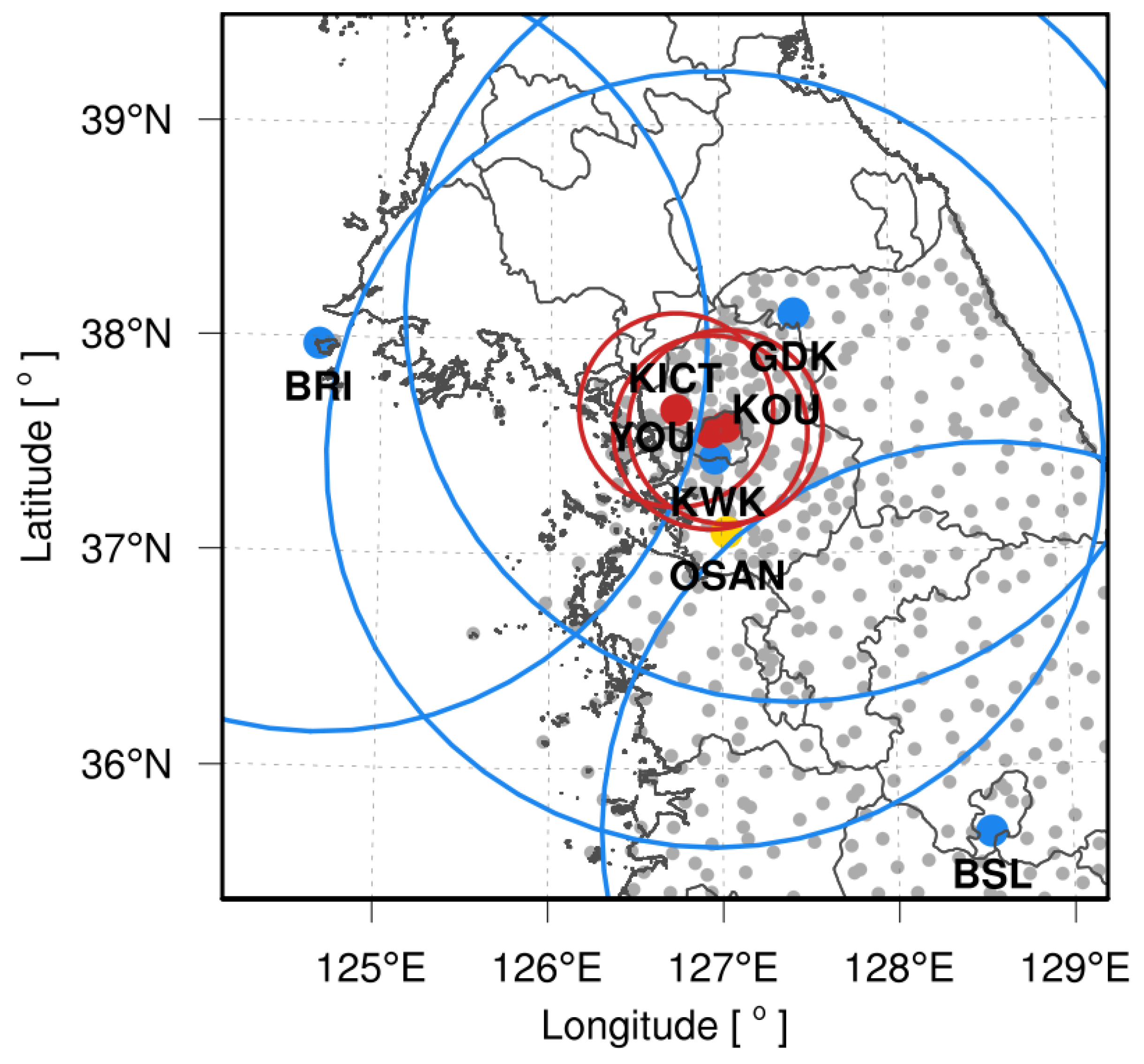
Figure 1 indicates the observation locations of the data that were used in this study. S-band radars on Baengnyeong Island (BRI), Kwanak Mountain (KWK), Gwangdeok Mountain (GDK), and Bisl Mountain (BSL), which are operated by the Korea Meteorological Administration (KMA) and the MOE and X-band radars (Korea Institute of Civil Engineering and Technology, KICT; Yonsei University, YOU; Korea University, KOU) in the Seoul metropolitan area were assimilated. We used the Kyungpook National University (KNU) fuzzy logic algorithm to perform a rigorous quality check (QC) on the radar data to remove the anomalous propagation (AP) of electromagnetic waves and non-meteorological echoes, such as ground clutter and chaffs [23]. Plan position indicator (PPI) data were quality-checked and processed to create radar CAPPI (constant altitude PPI) composite fields and interpolated onto a model grid of the same domain size and resolution as input fields (3 km for domain 2 and 1 km for domain 3). Surface AWS were assimilated to provide low-level observation information. AWS data were used within the model domain among 969 locations operated by the KMA (resolutions are the same as the CAPPI radar). Surface pressure, sea-level pressure, 10 min average wind speed and direction, temperature, and dew point temperature data were also interpolated onto a model grid. AWS precipitation data were used to verify the model’s accuracy, and Osan radiosonde data were used to verify the vertical profile of the atmospheric variables.

Table 1. Summary of observations used in this study.

Purpose	Observations	Variables	Horizontal Resolution	Vertical Resolution	Time Period	Time Resolution
Data assimilation	Radar	Reflectivity (dBZ), Doppler radial velocity (m·s−1)	1, 3 km *	200 m	3 h	30 min
	AWS	Surface pressure (hPa), sea level pressure (hPa), 10-min average wind speed (m·s−1) and direction (°), temperature and dew point temperature (K)		-
Verification		Precipitation (mm)	1 km *	-	9 h	1 h
	Radiosonde	Water vapor mixing ratio (g·kg−1), temperature (K), wind speed (m·s−1) and direction (°)	Point	50 hPa	0000 or 1200 UTC *

* Observations interpolated to model grid. UTC —Universal Coordinated Time.

summarizes the purpose, variables, and space–time resolutions of each observation used in this study.

In all three events considered, every 30 min, cycling of data assimilation is performed for 3 h, totaling six assimilation cycles. In each assimilation cycle, observations from radar reflectivity, radial velocity, and AWS observations are used.

2.2. WRF 3D-Var Assimilation System

The 3D-Var data assimilation method in WRF system is capable of assimilating all types of conventional observations, as well as radar data. The 3D-Var system combines the observations with background information on the model state and uses a linearized forecast model to ensure that the observations are given a dynamically realistic and consistent analysis field [10]. In this study, we used an incremental WRF 3D-Var data assimilation system [24,25]. The 3D-Var incremental system minimizes a scalar term called the cost function (or objective function, J), defined as a function of the analysis increment relative to the first gauss (background), using a linearized observation operator. The minimizations are subjected to the constraint of observation uncertainty, the difference between the observations, and the analysis projected to the observation space using the observations operator (H).

$$\mathrm{J}={\mathrm{J}}_{\mathrm{b}}+{\mathrm{J}}_{\mathrm{o}}=\frac{1}{2}{\nu }^T\nu +\frac{1}{2}\left(\mathrm{d}-{\mathrm{H}}^{\prime }\mathrm{U}\nu \right){\mathrm{R}}^{-1}\left(\mathrm{d}-{\mathrm{H}}^{\prime }\mathrm{U}\nu \right).$$

(1)

The terms J_o and J_b are the cost functions obtained from observation and background term, whereas R is the observation error covariance matrix. The term $\mathrm{d}={\mathrm{y}}_{\mathrm{o}}-\mathrm{H}\left({\mathrm{x}}_{\mathrm{b}}\right)$ is the innovation vector, which measures the departure of the observation ${\mathrm{y}}_{\mathrm{o}}$ and the background ${\mathrm{x}}_{\mathrm{b}}$, while ${\mathrm{H}}^{\prime }$ is the linearization of the nonlinear observation operator H. The term $\nu$ is the control variable, where $\nu ={\mathrm{U}}^{\prime }\left(\mathrm{x}-{\mathrm{x}}_{\mathrm{b}}\right)$, and U is the decomposition of the background error covariance B under the constrain $\mathrm{B}={\mathrm{UU}}^{\mathrm{T}}$. The covariance matrix for the regional background error statistics was calculated using National Meteorological Center (NMC) method [26] by taking 24 h and 12 h forecasts during the summer period (June, July, and August) for the chosen domain with five control variables. These are the stream function, unbalanced temperature, unbalanced surface pressure, unbalanced velocity potential, and pseudo-relative humidity. The minimization of cost is performed using the conjugate gradient method.

2.3. Radar Observation Operator

2.3.1. Radar Reflectivity Observation Operator

The radar reflectivity was partitioned into the reflectivity of each hydrometeor type based on the model background temperature by using the hydrometeor classification method and then converted to the hydrometeor mixing ratio.

The observed reflectivity (Z_o) was converted from dBZ to mm⁶·m⁻³, which is the unit for input reflectance (Z_e) and is expressed as

Z_o = 10 log₁₀ Z_e.

(2)

Z_e can be expressed as

Z_e = Z_r+ Z_ds+ Z_ws+ Z_g,

(3)

because it is a volume average that is observed by several hydrometeors, such as rain (r), dry snow (ds), wet snow (ws), and graupel (g) [27,28,29].

For the precipitation echo data assimilation (Z_o > −15 dBZ), Wang et al. (2013) classified hydrometeors by using the model’s temperature field (T (K)). Rain exists in a grid with a temperature of T ≥ 5 °C, and a grid temperature of −5°C < T < 5 °C assumes that rain, wet snow, hail, and dry snow can coexist (Equations (4)–(7)). The $\alpha$ in Equations (5)–(6) represents a value of zero at −5 °C with $\alpha$ = 1 at 5 °C, and it varies linearly between zero and one with the model temperature (Equation (8)).

Z_e = Z_r (5 °C ≤ T).

(4)

Z_e = α Z_r + (1 − α)[Z_ws + Z_g] (0 °C < T < 5 °C).

(5)

Z_e = α Z_r + (1 − α)[Z_ds + Z_g] (−5 °C < T < 0 °C).

(6)

Z_e = Z_ds + Z_g (T ≤ −5 °C).

(7)

$$\alpha =\frac{\mathrm{T}+5{}^{°}\mathrm{C}}{10{}^{°}\mathrm{C}}(-5{}^{°}\mathrm{C}<\mathrm{T}\le 5{}^{°}\mathrm{C}).$$

(8)

The reflectivity of the hydrometeors was converted into the mixing ratio (kg·kg⁻¹) of each hydrometeor by using the equation of the reflectivity–mixing ratio relationship. The hydrometeor mixing ratio was then used as an indirect assimilation method to assimilate reflectivity into the model [30].

$${\mathrm{q}}_{\mathrm{r}}={[{\mathrm{Z}}_{\mathrm{r}}({\rho }_{\mathrm{a}}\times {(3.63\times {10}^9)}^{-1}]}^{0.57},$$

(9)

$${\mathrm{q}}_{\mathrm{ws}}={[{\mathrm{Z}}_{\mathrm{ws}}({\rho }_{\mathrm{a}}\times {(4.26\times {10}^{11})}^{-1}]}^{0.57},$$

(10)

$$\mathrm{q}={[{\mathrm{Z}}_{\mathrm{ds}}({\rho }_{\mathrm{a}}\times {(9.80\times {10}^8)}^{-1}]}^{0.57},$$

(11)

$${\mathrm{q}}_{\mathrm{g}}={[{\mathrm{Z}}_g({\rho }_{\mathrm{a}}\times {(4.33\times {10}^8)}^{-1}]}^{0.57},$$

(12)

where $\rho$_a is the density (kg·m⁻³) of air. To create an environment in which convective clouds are actively maintained, the water vapor mixing ratio was nudged as the saturated water vapor mixing ratio when the observed reflectivity was greater than 30 dBZ. The saturated water vapor mixing ratio was calculated by using the Clausius–Clapeyron equation (e (hPa)) for water, and the water vapor saturation mixing ratio (q_s) was calculated as follows:

$$\mathrm{e}=6.112\times \exp [\frac{\mathrm{L}}{R_v}(\frac{1}{273.15}-\frac{1}{T})],$$

(13)

$${\mathrm{q}}_{\mathrm{s}}=\frac{ϵe}{p-\left(1-ϵ\right)e},$$

(14)

where L is 2.5 × 10⁶ J·kg⁻¹ by heat of evaporation, R_v represents the gas constant of water vapor (461.51 J·kg⁻¹·K⁻¹), $ϵ$ is the ratio of the gas constant of dry air to the gas constant of water vapor, and P (hPa) is the pressure of the model.

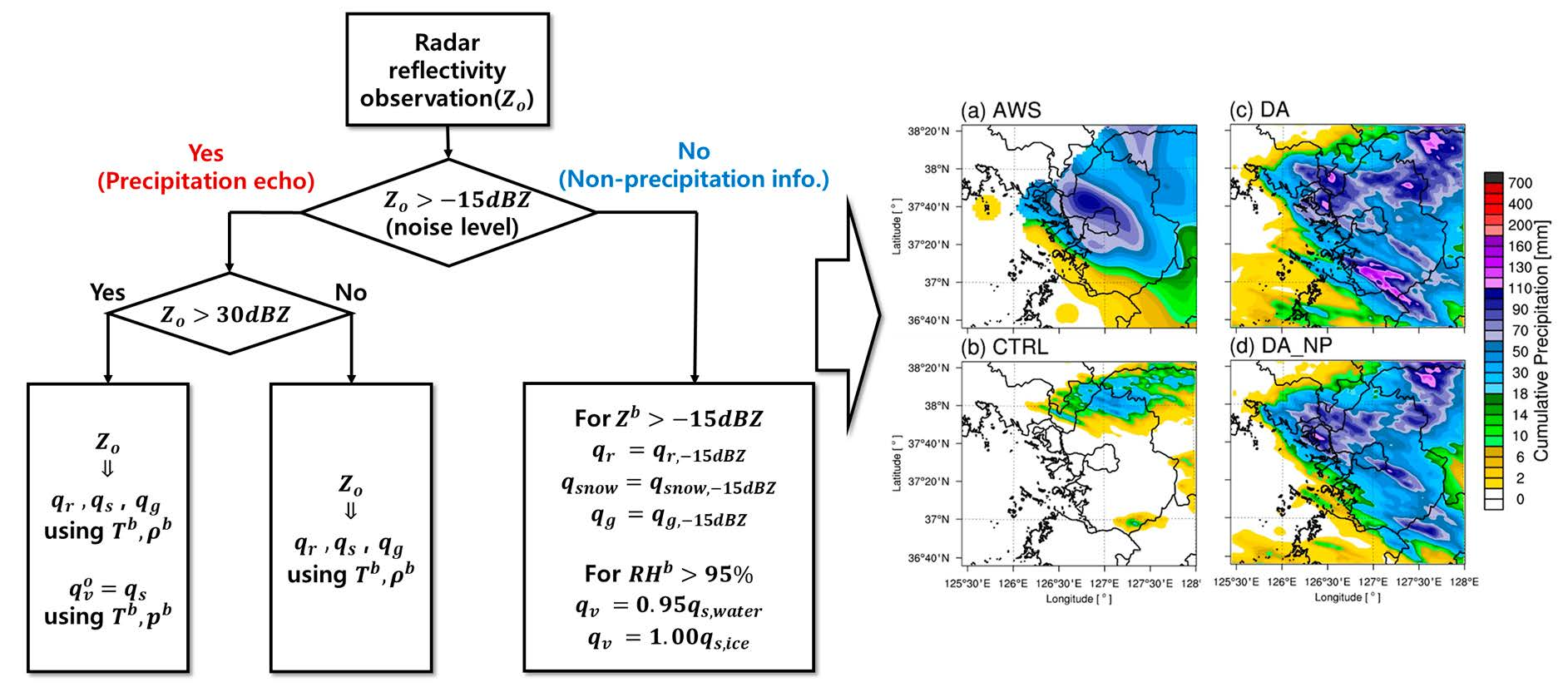
For the null-echo data assimilation with the observed Z_o < −15 dBZ, we substituted Z_e into Equations (9)–(12) with −15 dBZ when the model background reflectivity (Z_b) exceeded −15 dBZ and the corresponding value for each hydrometeor mixing ratio (q_x), which is expressed as

q_r = q_r,noise      Z_o < −15 dBZ, Z_b > −15 dBZ,

(15)

q_snow = q_snow,noise      Z_o < −15 dBZ, Z_b > −15 dBZ,

(16)

q_g = q_g,noise       Z_o < −15 dBZ, Z_b > −15 dBZ.

(17)

We assumed that only liquid clouds existed when the temperature of the model background was larger than or equal to 5 °C. In this criterion, the relative humidity for water vapor in the model (RH^b) was reduced to 95% when close to saturation. Assuming mostly solid cloud particles when the temperature was less than or equal to −5 °C, only the super saturated water vapor mixing ratio was removed. If the temperature of the background was between −5 °C and 5 °C, the two preceding criteria were mixed and added linearly according to the temperature of the background. In other words, no precipitation except clouds remained in the atmosphere.

$${\mathrm{q}}_{\mathrm{v}}=0.95\times {\mathrm{q}}_{\mathrm{s},\mathrm{water}}5{}^{°}\mathrm{C}\le \mathrm{T},$$

(18)

$${\mathrm{q}}_{\mathrm{v}}=\alpha (0.95\times {\mathrm{q}}_{\mathrm{s},\mathrm{water}})+(1-\alpha \left)\right(1.00\times {\mathrm{q}}_{\mathrm{s},\mathrm{ice}})-5{}^{°}\mathrm{C}<\mathrm{T}<5{}^{°}\mathrm{C},$$

(19)

$${\mathrm{q}}_{\mathrm{v}}=1.00\times {\mathrm{q}}_{\mathrm{s},\mathrm{ice}}\mathrm{T}\le -5{}^{°}\mathrm{C}.$$

(20)

The saturation mixing ratio for ice was obtained by using Equation (13) for ice (L is 2.83 × 10⁶ J·kg⁻¹, the latent heat of sublimation), and the water vapor pressure for ice was calculated with Equation (14). A schematic diagram for assimilating radar reflectivity with null-echo information is shown in Figure 2.

2.3.2. Doppler Radial Velocity Observation Operator

To assimilate the Doppler radar radial velocity (V_r), the wind variable of the model is converted to the Doppler radial velocity.

$${\mathrm{V}}_{\mathrm{r}}=\mathrm{u}\frac{\mathrm{x}-{\mathrm{x}}_{\mathrm{i}}}{{\mathrm{r}}_{\mathrm{i}}}+\mathrm{v}\frac{\mathrm{y}-{\mathrm{y}}_{\mathrm{i}}}{{\mathrm{r}}_{\mathrm{i}}}+\left(\mathrm{w}-V_T\right)\frac{\mathrm{z}-{\mathrm{z}}_{\mathrm{i}}}{{\mathrm{r}}_{\mathrm{i}}},$$

(21)

where u, v, and w (m·s⁻¹) are the wind components of the model, x, y, and z are the locations of the radars, x_i, y_i, and z_i are the locations of the radar observation data, r_i (m) is the distance between the radar and the observation point, and V_T (m·s⁻¹) is the terminal velocity. Sun and Crook (1998) terminal velocity equation was used to relate rainwater mixing ratio to V_T (Equation (22)) [31].

$${\mathrm{V}}_{\mathrm{T}}=5.40{\mathrm{aq}}_{\mathrm{r}}^{0.125},$$

(22)

where q_r is the rainwater mixing ratio (kg·kg⁻¹), and a is correctional term calculated using Equation (23).

$$\mathrm{a}={\left(\frac{{\mathrm{p}}_0}{\overline{\mathrm{p}}}\right)}^{0.4},$$

(23)

where ${\mathrm{p}}_0$ is ground pressure, and $\overline{\mathrm{p}}$ is state pressure (Pa). More detailed information on how the operator of Equation (21) is connected to the control variables can be found in Xiao et al. (2005) [22].

2.4. Model Configuration and Experimental Design

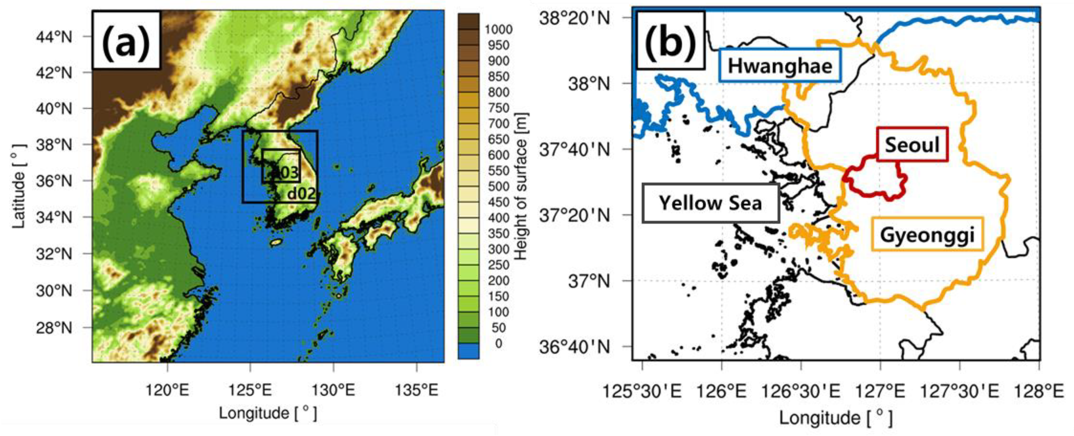
This study was conducted by using the WRF version 3.9.1 model, which was developed by the National Center for Atmospheric Research (NCAR) [32]. As shown in Figure 3, this model consisted of three nesting domains with resolutions of 9 km, 3 km, and 1 km, and it was centered over the Seoul metropolitan area, where heavy rainfall occurred. Cumulus parameterization was applied to all areas because the Multiscale Kain–Fritsch Scheme suitable for high-resolution models was used [33]. The WRF Double Moment 6 class (WDM6) scheme was employed for cloud microphysics processes, and the planetary boundary layer (PBL) used the Yonsei university (YSU) scheme [34,35]. A rapid radiative transfer model (RRTM) was selected for long-wave processes, and the Dudhia short-wave scheme was selected for short-wave processes [36,37]. Surface layer processes used the revised MM5 Monin–Obukhov scheme, and land surface processes utilized the Unified Noah land surface model [38,39]. The initial and boundary conditions were based on the NCEP GFS 0.25 Degree Global Forecast Grids Historical Archive, which has a resolution of 0.25° and was provided by the National Centers for Environmental Prediction/National Centers for Atmospheric Research (NCEP/NCAR). The model configurations are summarized in

Table 2. Summary of the Weather Research and Forecasting (WRF) v3.9.1 model configurations.

	D01	D02	D03
Resolution	9 km	3 km	1 km
Number of Grids	240 × 240 × 60	151 × 151 × 60	226 × 196 × 60
Cumulus	Multiscale Kain–Fritsch scheme
Microphysics	WRF Double Moment 6 class scheme
Planetary Boundary Layer	Yonsei University Scheme
Surface Layer	Revised MM5 Monin–Obukhov scheme
Land Surface	Unified Noah land surface model
Long-Wave Radiation	Rapid radiative transfer model scheme
Short-Wave Radiation	Dudhia scheme
Initial and Boundary Conditions	National Center for Environmental Prediction Global Forecast System 0.25 Degree Historical Archive

.

Three experiments were performed to compare the effects of data assimilation and null-echo data assimilation (

Table 3. Experimental design.

	Assimilated Observation Data
CTRL	No data assimilation
DA	AWS + radar radial velocity + radar reflectivity
DA_NP	AWS + radar radial velocity + radar reflectivity + null echoes

). The first experiment, the CTRL experiment, generated a 12 h forecast by using only the initial and boundary conditions without performing any data assimilation. The CTRL was set as a measure of the degree of improvement for the data assimilation experiments. The second experiment, referred to as DA, involved data assimilation as performed in the majority of studies with experiments that assimilate AWS data with radar radial velocities and precipitation echoes. The third experiment, DA_NP, further assimilated null-echo information into the model that already included precipitation echoes from DA. These two experiments (DA and DA_NP) assimilated observations into domains 2 and 3 for 3 h with cycling intervals of 30 min totaling six times, and a 9 h forecast field was created. This avoids the need for thinning the input data and allows more radar and AWS data to be used in the model since the data are interpolated in the pre-processing stage. Furthermore, it can reduce the moisture inconsistency between domain 2 and domain 3 that can lead to forecast degradation when two-way nesting is applied.

2.5. Description of the Cases

Three cases of heavy rainfall over the Seoul metropolitan area were selected to understand the predictability of NWP model forecasts with radar DA. These three cases were typical summertime convective systems along the Changma front in Korea. The forecast periods and characteristics of these cases are summarized in

Table 4. Selected cases for the numerical experiments and their storm characteristics.

	Forecast Period		Total Cumulative Precipitation (mm)	Maximum Rain Rate (mm·h−1)	Maximum CAPE * (J·kg−1)
	CTRL	DA and DA_NP
Case 1	2017.07.02.0600 UTC ~ 1800 UTC	2017.07.02.0900 UTC ~ 1800 UTC	55	55.0	1233
Case 2	2017.07.22.1800 UTC ~ 2017.07.23.0600 UTC	2017.07.22.2100 UTC ~ 2017.07.23.0600 UTC	110	67.0	1521
Case 3	2018.08.28.0600 UTC ~ 1800 UTC	2018.08.28.0900 UTC ~ 1800 UTC	180	73.0	1468

* CAPE—Convective Available Potential Energy

.

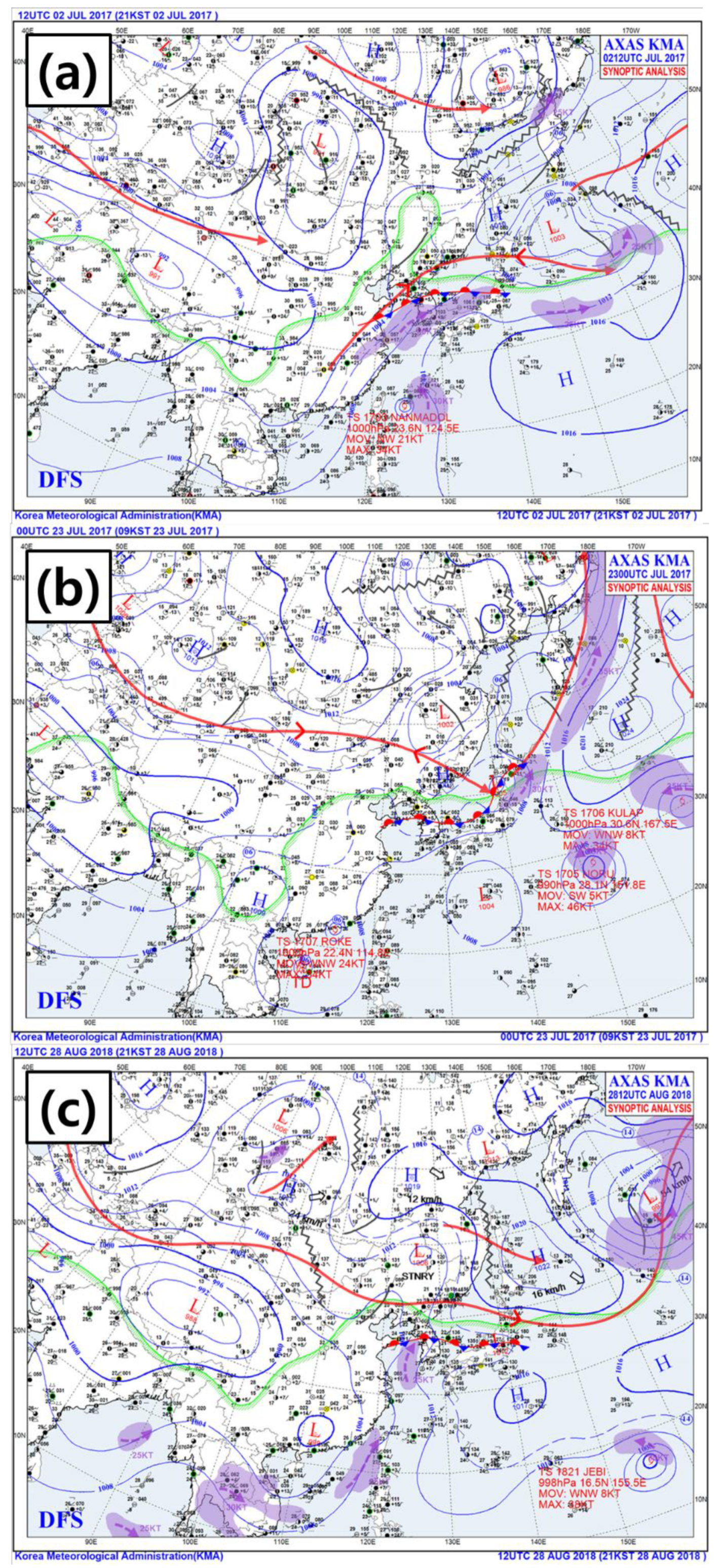
On 2 July 2018 (Case 1), the upper level trough (gray line) approached from the north, causing the atmosphere to become unstable (Figure 4a), and a large quantity of water vapor in the East China Sea moved into the Yellow Sea along the low-level jet (purple zones). The system had a typical Changma front signature during the summer monsoon period. The Seoul metropolitan area received 55.0 mm·h⁻¹ of rain. Similarly, on 22 July 2017 (Case 2), baroclinic instability that was created by an upper level trough and a pocket of cold air induced 67.0 mm·h⁻¹ of heavy rainfall during the case period (Figure 4b). On 28 August 2018 (Case 3), high pressure in the North Pacific extended westward and the monsoon front moved north with a low-level jet located in the West Sea (Figure 4c). Water vapor moved into the West Sea from the East China Sea along the low-level jet, and 4 × 10⁻⁵ s ⁻¹ of convergence occurred (not shown). This event caused another convective system along the Changma front. The convective system moved along the stationary monsoon front, causing up to 73.0 mm·h⁻¹ of heavy rainfall in the Seoul metropolitan area.

2.6. Evaluation Parameters

2.6.1. Accuracy Verification

For an objective comparison of the forecasts, we considered a couple of evaluation parameters as described below. Quantitative error verification was performed by using the cumulative precipitation from AWS data and the model simulations. The mean absolute error (MAE) and root-mean-square error (RMSE) can be defined as in Equations (24)–(26).

$$\mathrm{Bias}={\mathrm{P}}_{\mathrm{i}}-{\mathrm{O}}_{\mathrm{i}},$$

(24)

$$\mathrm{MAE}=\frac{1}{{\mathrm{N}}_{\mathrm{k}}}{\sum }_{i=1}^n\left|{\mathrm{P}}_{\mathrm{i}}-{\mathrm{O}}_{\mathrm{i}}\right|,$$

(25)

$$\mathrm{RMSE}=\sqrt{\frac{1}{{\mathrm{N}}_{\mathrm{k}}}{\sum }_{i=1}^n{\left({\mathrm{P}}_{\mathrm{i}}-{\mathrm{O}}_{\mathrm{i}}\right)}^2},$$

(26)

where ${\mathrm{P}}_{\mathrm{i}}$ is the predicted precipitation (mm), ${\mathrm{O}}_{\mathrm{i}}$ is the observed precipitation from AWS (mm), and N is the number of horizontal grids in the model.

Verification was performed to evaluate the occurrence of model precipitation compared to the AWS observations. A contingency matrix for skill score calculations is shown in

Table 5. Contingency table matrix (2 × 2) for skill score calculations.

		Observation		Total
		Yes	No
Forecast	Yes	Hits = A	False alarms = B	Forecast Yes
	No	Misses = C	Correct negative = D	Forecast No
Total		Observed Yes	Observed No	Total = N

.

Accuracy determines whether the same forecast or non-forecast occurred, as expressed in Equation (27). Values closer to one indicate higher accuracy.

$$\mathrm{Accuracy}=\frac{\mathrm{A}+\mathrm{D}}{\mathrm{A}+\mathrm{B}+\mathrm{C}+\mathrm{D}}.$$

(27)

The critical success index (CSI) is an indicator that focuses on accurately predicting precipitation. The ratio of precipitation prediction (Equation (28)) is sensitive to A and becomes lower when B and C occur. A perfect prediction of precipitation has a value of one.

$$\mathrm{CSI}=\frac{\mathrm{A}}{\mathrm{A}+\mathrm{B}+\mathrm{C}}.$$

(28)

The equitable threat score (ETS) is similar to the CSI but removes the contribution from S_f (Equation (29)), which is an accidental hit, with higher accuracy approaching one (Equation (30)).

$${\mathrm{S}}_{\mathrm{f}}=\frac{\left(\mathrm{A}+\mathrm{C}\right)\left(\mathrm{A}+\mathrm{B}\right)}{\left(\mathrm{A}+\mathrm{B}+\mathrm{C}+\mathrm{D}\right)}.$$

(29)

$$\mathrm{ETS}=\frac{\mathrm{A}-{\mathrm{S}}_{\mathrm{f}}}{\mathrm{A}+\mathrm{B}+\mathrm{C}-{\mathrm{S}}_{\mathrm{f}}}.$$

(30)

2.6.2. Space- and Time-Averaged Comparison Fields

(a) Contoured Frequency by Altitude Diagram (CFAD)

A CFAD is a contour plot that displays the frequency distribution of reflectivity in an area of detectable echo volume at each vertical height. Many studies showed that CFADs are a convenient tool to examine the characteristics of storms, especially in terms of their temporally averaged evolution [40,41,42,43]. Min et al. (2015) showed that CFADs can assess the characteristics of microphysics schemes in simulating summer monsoon and convective precipitation using radar observations [43].

A CFAD begins with a histogram calculation that uses a constant reflectivity bin width within a constant vertical volume. The CFAD ignores the horizontal echo structure and summarizes the frequency distribution information in a single two-dimensional plot. In this study, the radar and simulated reflectivity of the CFAD was −16 dBZ or greater, with a bin width of 0.5 dBZ and vertical intervals of 250 m. The histograms were normalized by the total number of points at each vertical level, and the results were converted into percentage values. The average reflectivity (dBZ1) and the average of the reflectivity factor in linear units (dBZ2, in mm⁻⁶·m⁻³) for each height were calculated as follows:

$$\mathrm{dBZ}1\mathrm{k}=\frac{1}{{\mathrm{N}}_{\mathrm{k}}}{\sum }_{i=1}^n{\mathrm{dBZ}}_{\mathrm{i}},$$

(31)

$$\mathrm{dBZ}2\mathrm{k}=10\times {\log }_{10}\left(\frac{1}{{\mathrm{N}}_{\mathrm{k}}}{\sum }_{i=1}^n{10}^{0.1\times {\mathrm{dBZ}}_{\mathrm{i}}}\right),$$

(32)

where N is the total number of points at each height (level). The linear unit reflectivity factor was used to better identify the location of the bright band (BB). This phenomenon is caused by melting ice particles through the 0 °C isotherm layer. In addition, we calculated the cumulative reflectivity frequencies of the 25th, 50th, and 75th percentiles, which were included in each of the CFAD plots.

(b) Time–Height Cross-Sections (THCS)

A time–height cross-section diagram is useful to identify the duration of precipitation and the various echo tops of the precipitating system [43]. This type of diagram is used to augment CFADs, which do not reveal the time evolution characteristics of reflectivity (i.e., precipitation) that are related to phase errors when simulating any storm. We calculated the THCS of the simulated reflectivity with a 1 h temporal resolution, whereas the radar observations had 20 min resolution (temporal). Additionally, all the observed datasets were vertically interpolated to 250 m from their native polar and model sigma vertical coordinates to the same vertical resolution. The range was limited to an approximately 100,000-m radius. The melting level in the time–height cross-section is represented by a dashed line that stretches horizontally with higher reflectivity below the neighboring area.

3. Results

3.1. Increment of the Analysis Field

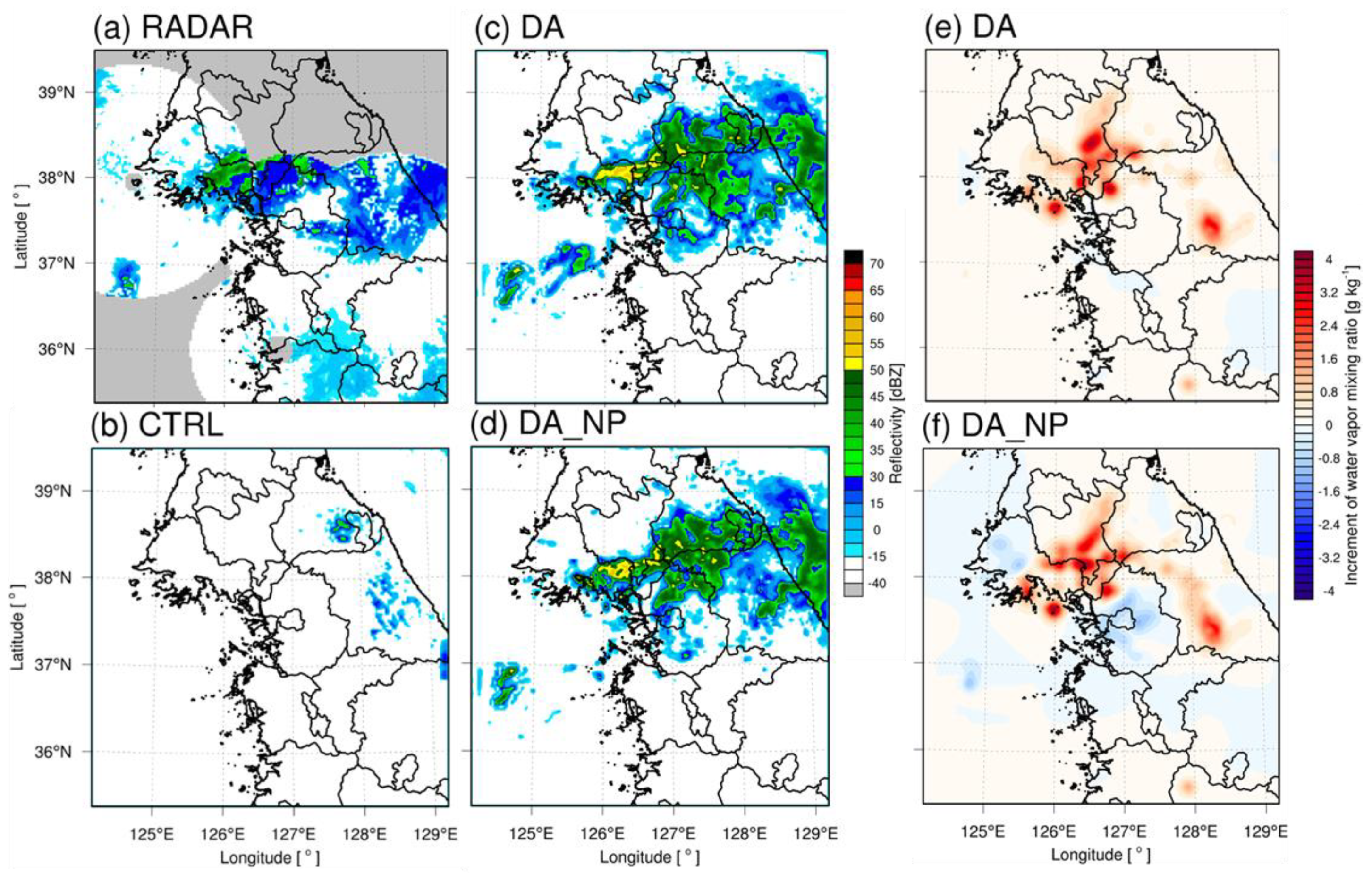
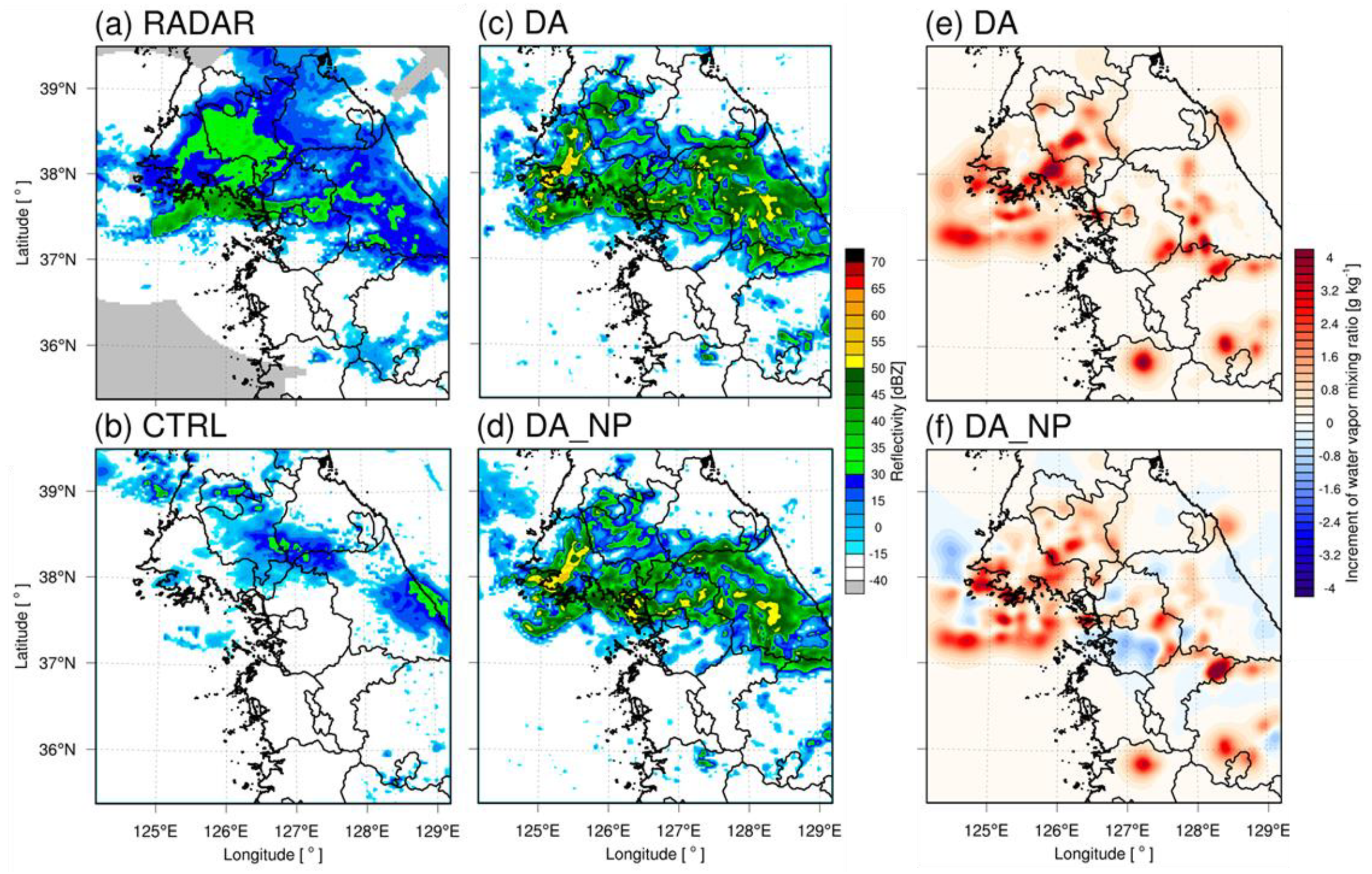
The predicted accuracy of a numerical forecast model depends on the fidelity of the analysis field. The horizontal increments of the DA and DA_NP analysis fields at the last cycle time were analyzed to understand changes in the analysis fields following the assimilation experiments. Figure 5, Figure 6 and Figure 7 show the radar, CTRL, DA, and DA_NP reflectivity (dBZ) and increments of the water vapor mixing ratio (g·kg⁻¹) for DA and DA_NP at 2.0 km above sea level. Figure 5 shows the results for 0900 UTC 2 July 2017. Reflectivity greater than 30 dBZ was observed in the West Sea and inland areas of the Korean Peninsula. The CTRL simulated reflectivity greater than 30 dBZ over the West Sea, but its area was smaller than that of the observations. DA and DA_NP, which included data assimilation, simulated greater reflectivity over the West Sea than the CTRL and were closer to the observations. The water vapor mixing ratio increased where the reflectivity was located in DA and DA_NP because of the effect of radar data assimilation. No water vapor reduction occurred in DA_NP because no over-simulated reflectivity was observed in the region where the reflectivity was below −15 dBZ. On 2100 UTC 22 July 2017, reflectivity greater than 30 dBZ was observed along the demilitarized zone (DMZ), and DA and DA_NP simulated reflectivity above 30 dBZ in the same area but the CTRL never simulated reflectivity (Figure 6). The water vapor mixing ratio in DA and DA_NP increased in the area where the precipitation echo was located. Reflectivity below −15 dBZ was dominant in central Gyeonggi Province and Seoul. However, DA overestimated echoes above 30 dBZ. Because of the null-echo data assimilation, the water vapor mixing ratio of DA_NP was reduced to eliminate over-simulated reflectivity. At 0900 UTC 28 August 2018, over 30 dBZ of a well-defined precipitation echo along the frontal boundary (the Changma front) was observed in the West Sea (Figure 7). The CTRL did not simulate the arc-shaped echoes that developed and migrated over the West Sea. In contrast, DA and DA_NP simulated these arc-shaped echoes. However, echoes that did not exist in the radar observations were simulated in southern Gyeonggi because echoes were over-predicted in DA and DA_NP. In DA_NP, the water vapor mixing ratio was reduced after assimilating non-precipitation echo data.

3.2. Distribution of the Cumulative Precipitation

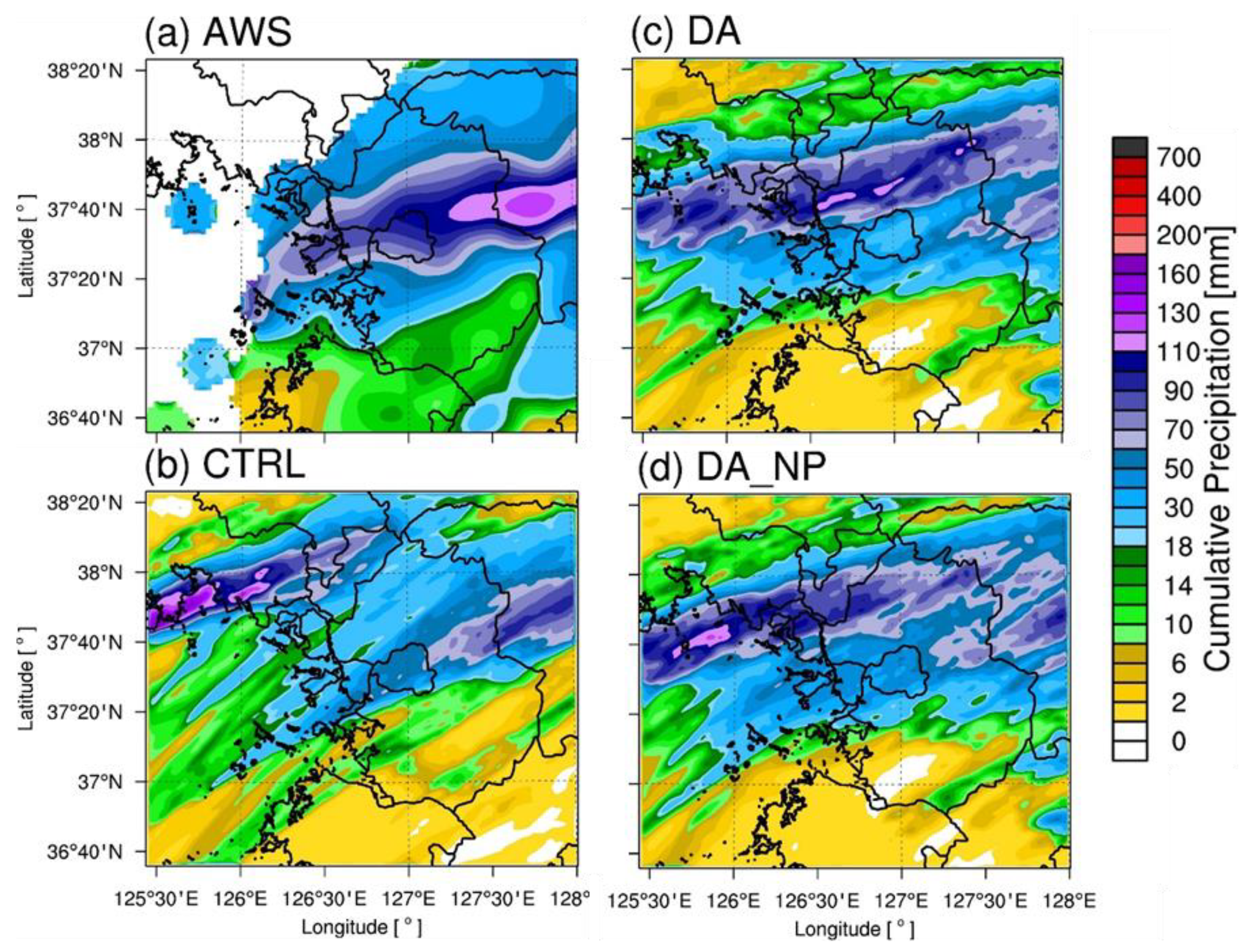
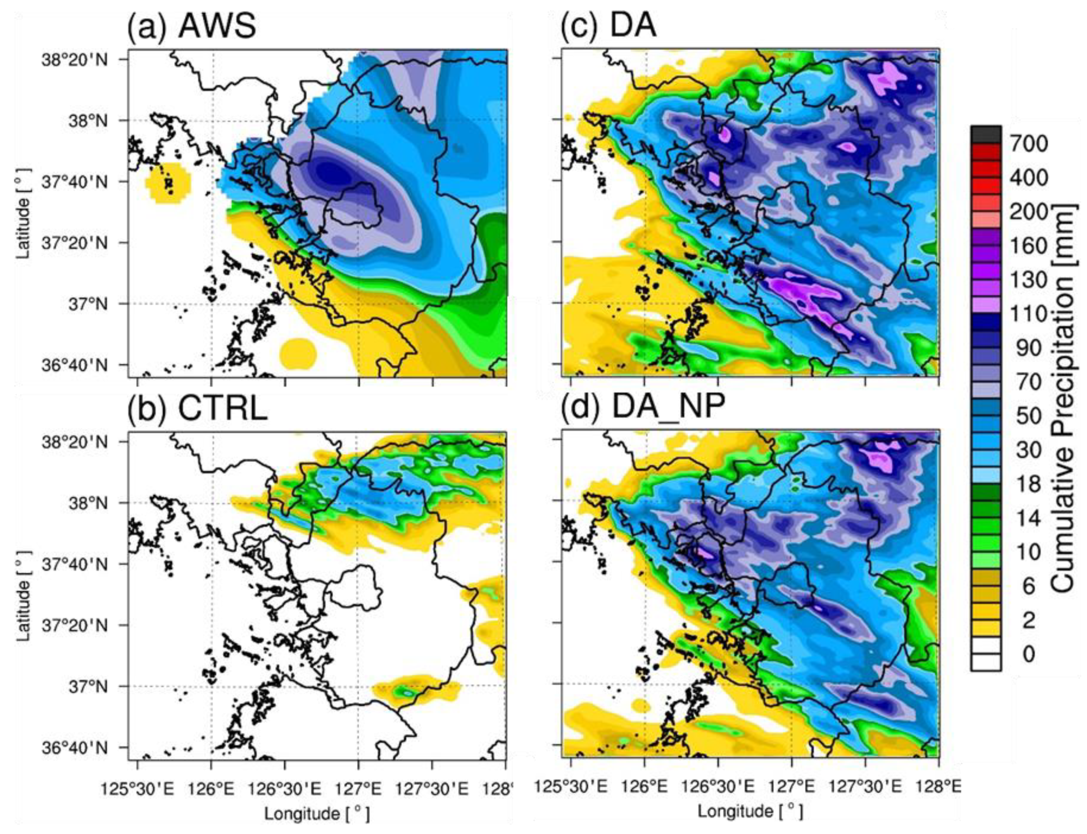
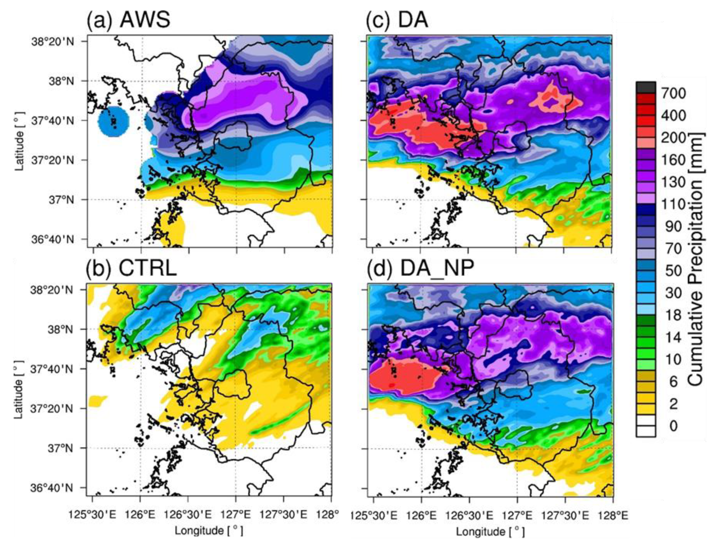
The distribution of the cumulative precipitation for each case is shown and analyzed for Cases 1, 2, and 3. Figure 8 shows the 9 h cumulative precipitation distribution of the AWSs, CTRL, DA, and DA_NP for Case 1. During this 9 h period, a narrow and elongated precipitation band of more than 100 mm was observed from the western to eastern metropolitan area. The CTRL simulated some precipitation but underestimated the amount and could not accurately simulate heavy rainfall. DA simulated heavy rain over 110 mm from the west to east and simulated similar precipitation patterns to the AWSs. However, the precipitation areas were further north than those of the AWSs and did not simulate heavy rain over 110 mm to the east of Gyeonggi. DA_NP reduced over-precipitation over 110 mm in the northeastern portion of Gyeonggi, but the precipitation area was still farther north compared to the observations, and this model did not simulate heavy precipitation to the east of Gyeonggi. Figure 9 shows the 9 h cumulative precipitation distribution for Case 2. The convective system moved from the northwest to the southeast, dropping more than 100 mm of heavy rain. The CTRL experiment failed to simulate precipitation in the metropolitan area. DA simulated precipitation in the Seoul metropolitan area, and its observed precipitation distribution was more similar to that of the AWSs compared to the CTRL. However, the precipitation amount increased, overestimating the intensity by more than 160 mm to the south of Gyeonggi. In contrast, DA_NP simulated over 100 mm of precipitation in the Seoul area, similarly to the observations, and removed the over-predicted precipitation from DA. Figure 10 shows the cumulative precipitation distribution for Case 3. As the convective system moved eastward, more than 100 mm of precipitation occurred in the metropolitan area. The CTRL did not correctly simulate the convective system and simulated less than 10 mm of precipitation in the Seoul metropolitan area. DA simulated more than 180 mm for the major precipitation structure but overestimated the amount in the Seoul area by 50 mm compared to the observations. With DA_NP, the null-echo data assimilation simulated approximately 90 mm of precipitation, similarly to the observations in the Seoul metropolitan area. In the DA and DA_NP experiments, there are areas of 200 mm or greater precipitation to the West Coast that were overestimated in the model. The over-prediction occurred immediately after the cycling, which was caused by excessive amount of water vapor and hydrometeor contents due to radar data assimilation.

3.3. Model Verification

Accuracy verification of the rainfall prediction was performed by using quantitative error verification and categorical precipitation classification (Table 5). The AWSs in South Korea have an effective radius of approximately 10 km². Thus, the average value of nine model precipitation grid points was compared to the closest AWS location in domain 3.

Table 6. Cumulative precipitation error for CTRL, DA, and DA_NP.

	Experiment	Bias (mm)	MAE (mm)	RMSE (mm)
Case 1	CTRL	−15.3	19.2	28.6
	DA	−9.1	20.0	30.0
	DA_NP	−8.8	18.2	26.7
Case 2	CTRL	−31.4	34.0	47.3
	DA	12.1	28.8	40.0
	DA_NP	2.3	21.3	31.4
Case 3	CTRL	−48.5	48.7	62.7
	DA	17.5	31.2	43.6
	DA_NP	2.8	23.3	35.4
Average	CTRL	−31.7	34.0	46.2
	DA	6.9	26.7	37.9
	DA_NP	−1.2	20.9	31.2

shows the model bias, MAE, and RMSE that were calculated by using the accumulated precipitation of the AWSs and forecast fields for each case. In all three cases (Cases 1–3), the CTRL showed negative bias after underestimating the precipitation location and intensity. However, the precipitation in the DA and DA_NP experiments was simulated through radar data assimilation, and the model bias, MAE, and RMSE were reduced compared to those of the CTRL. DA_NP showed the lowest error in all three cases (Cases 1–3), with excessively simulated water vapor and hydrometeors removed through null-echo data assimilation, simulating less precipitation than DA. The results of averaging the errors in all cases showed that the bias error was the greatest in the CTRL (−31.7 mm), and the precipitation in DA formed through data assimilation, but the bias of 6.9 mm indicates overestimated precipitation. DA_NP showed the lowest error rates, i.e., −1.2 mm for the bias, 20.9 mm for the MAE, and 31.2 mm for the RMSE, because of a reduction in the overestimated rainfall amount compared to DA.

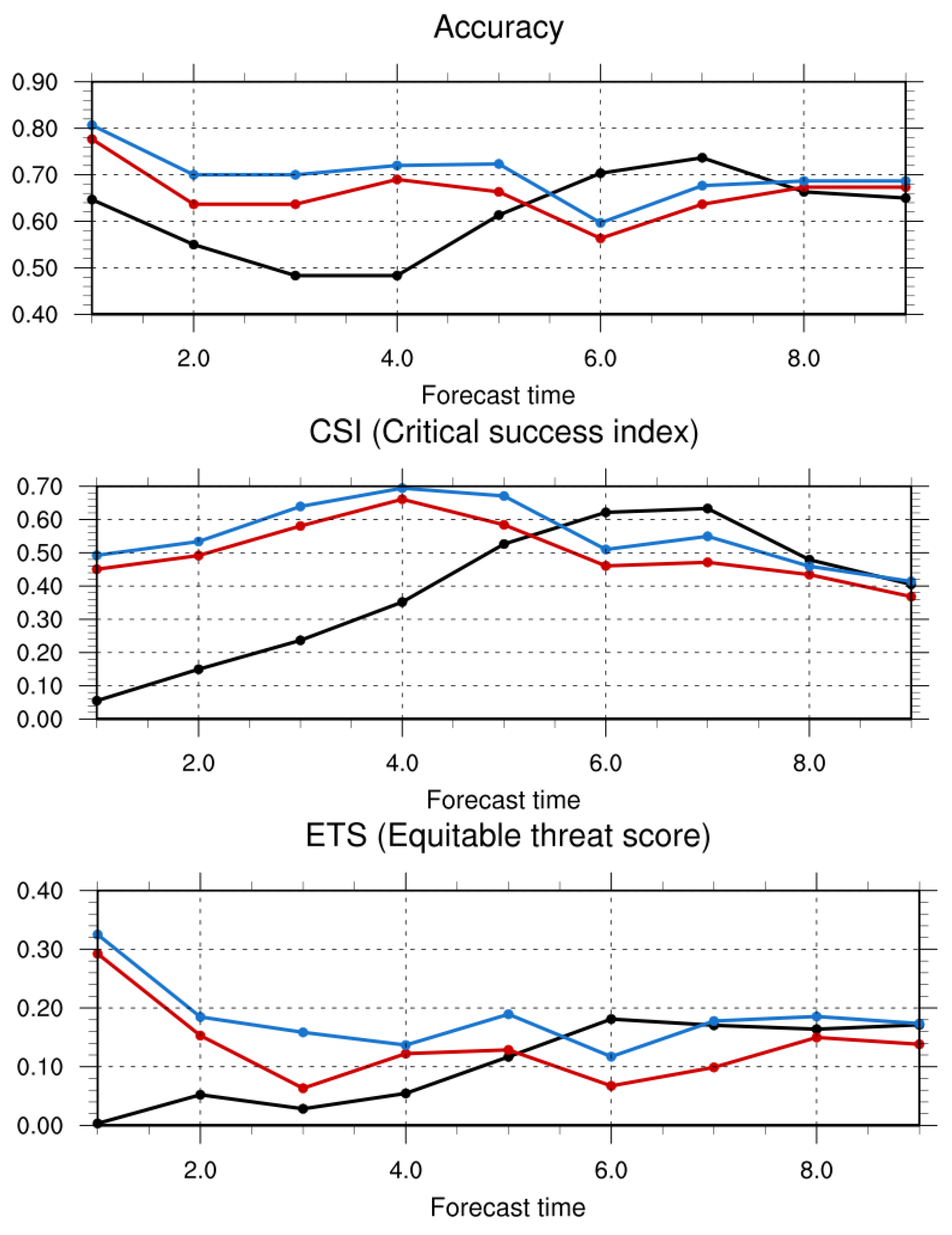
The categories were also verified according to the occurrence of precipitation. The categorical validation calculated the accuracy, CSI, and ETS as verification statistics depending on whether the observational data from the AWSs and model experiments detected precipitation. The accuracy, CSI, and ETS were obtained for the three cases and averaged over time (Figure 11). The effect of data assimilation continued for up to 6 h, and all three verification scores showed higher accuracy for DA and DA_NP compared to the CTRL. In DA_NP, the overestimated precipitation was reduced through null-echo data assimilation, showing the highest predicted accuracy. After 6 h, the verification scores in the experiment in which data assimilation was performed decreased because the overestimated rainfall amount increased the false alarm ratio (not shown).

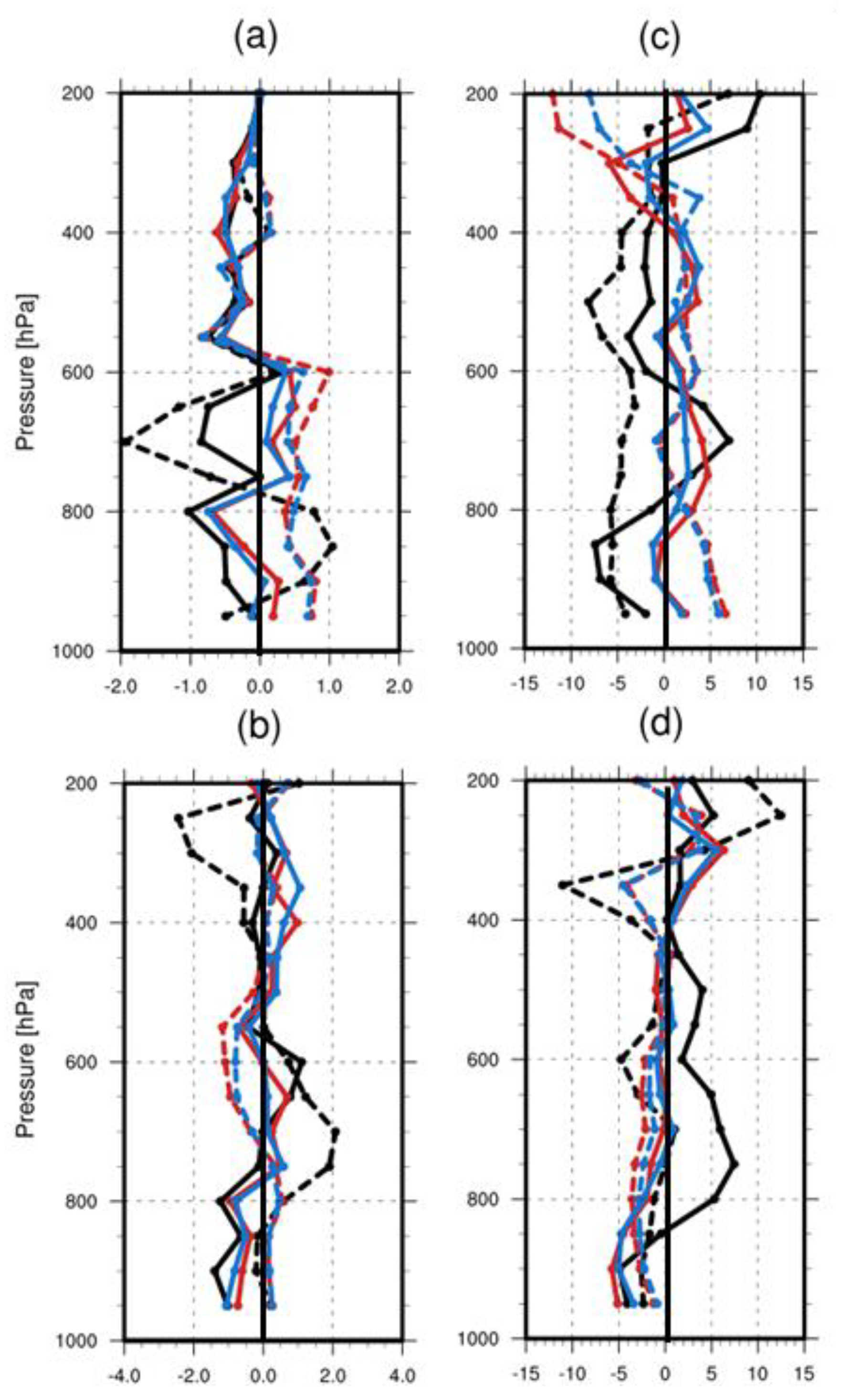
Vertical profile verification of 3 h prediction was performed by using Osan radiosondes. Figure 12 shows the biases of the water vapor mixing ratio, temperature, and wind components of the models compared to the Osan radiosonde data. No radiosonde data were available for Case 2, so only Case 1 and Case 3 were validated. In both cases, an underestimated water vapor mixing ratio was obvious in the CTRL from 600 hPa to 800 hPa. DA overestimated the water vapor mixing ratio, while DA_NP reduced the over-predicted mixing ratio by assimilating the null-echo data assimilation. Radar data assimilation improved the temperature profiles and showed lower error in DA and DA_NP compared to the CTRL. The effect of radial velocity data assimilation also improved the wind forecasts compared to the radiosonde data.

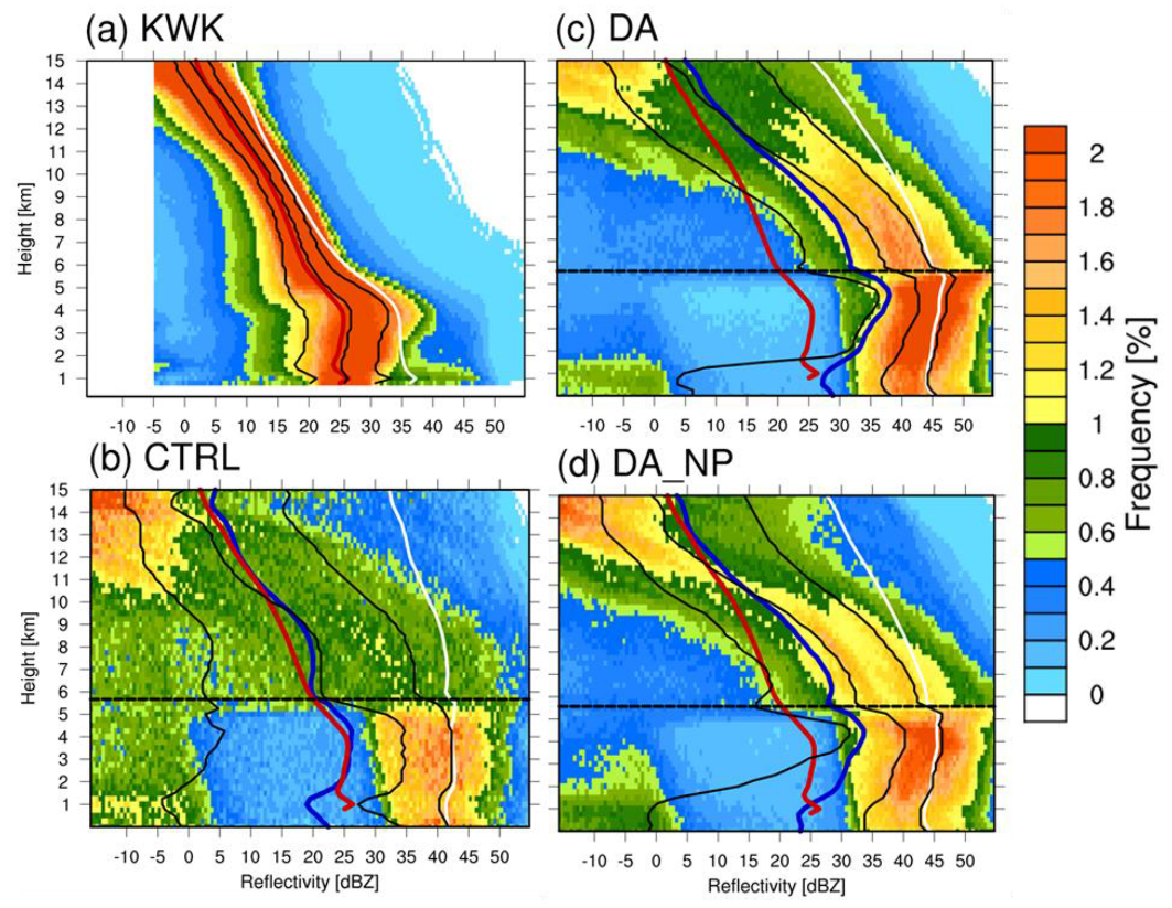
3.4. CFADs

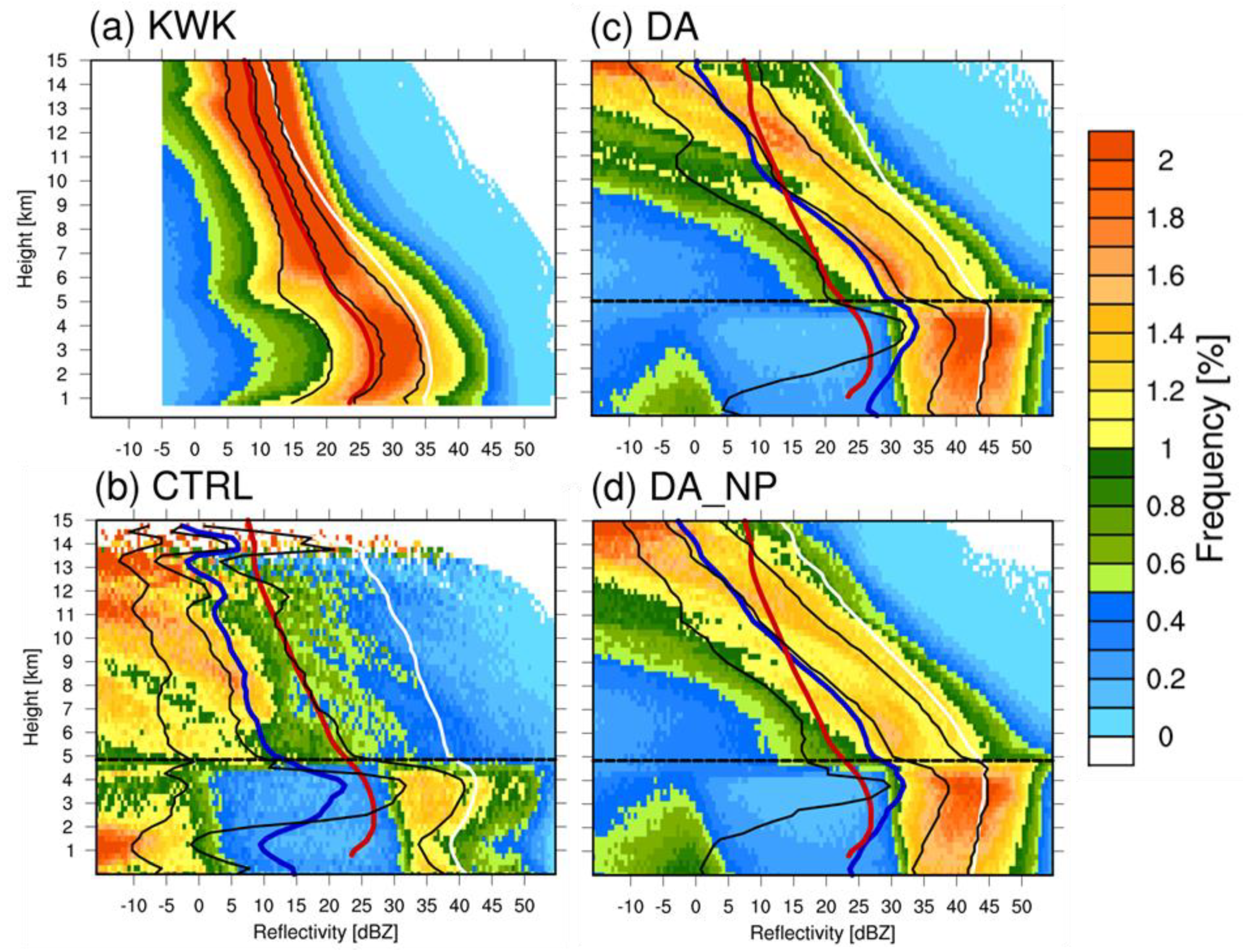
The CFADs of Cases 2 and 3 were analyzed only because Case 1 did not show significant effects from data assimilation. CFAD analysis was performed to analyze the microphysical development of precipitation. Both the radars and the models used reflectivity information within 100 km of the KWK location. Figure 13 shows a cumulative 9 h CFAD for the KWK radar site and the CTRL, DA, and DA_NP experiments. The CFAD of KWK shows that ice particles fell and grew from the upper level as the reflectivity increased with lower altitude. A strong reflectivity peak appeared at an altitude of 4 km, which is the location of the BB, and the growth of particles in the troposphere was adequately demonstrated. On the other hand, the CTRL hardly simulated precipitation; thus, no apparent microphysical structure was visible. In DA and DA_NP, ice particles fell and grew from the upper level, showing the highest frequency around 4.5 km below the melting layer at 5.5 km (dashed line). In the experiment in which data assimilation was performed, the reflectivity value was higher than the observed value for KWK, and the 50% line was shifted to the right. These results were caused by the double moment characteristics of WDM6, which employs a double moment only for liquid water droplets and, thus, tends to create a sharp increase in radar reflectivity below the melting level of 0 °C [42]. Thus, this model tends to overestimate the reflectivity compared to radar observations. The average reflectivity below the melting layer in DA_NP decreased by 5 dBZ compared to DA, showing a similar value to that of the observations. This phenomenon resulted from a reduction in water vapor and hydrometeors from the null-echo data assimilation. Figure 14 is the accumulated 9 h CFAD for Case 3. The CTRL simulation again failed to simulate the convective system; thus, the structure of hydrometeors growing from the top level did not appear. The data assimilation in DA and DA_NP increased the reflectivity from the upper level, showing the growth of hydrometeors, with the greatest reflectivity below the melting layer, a similar pattern to the observations. However, Case 3 also overestimated the reflectivity because of the inaccuracy of the microphysics scheme in simulating convective storms and the assimilation method of radar data, as noted in Case 2. DA_NP reduced the reflectivity of the 50% cumulative line below the melting layer by eliminating the mixing ratio of excessively simulated water vapor and hydrometeors in the model.

3.5. Time–Height Cross-Sections (THCS)

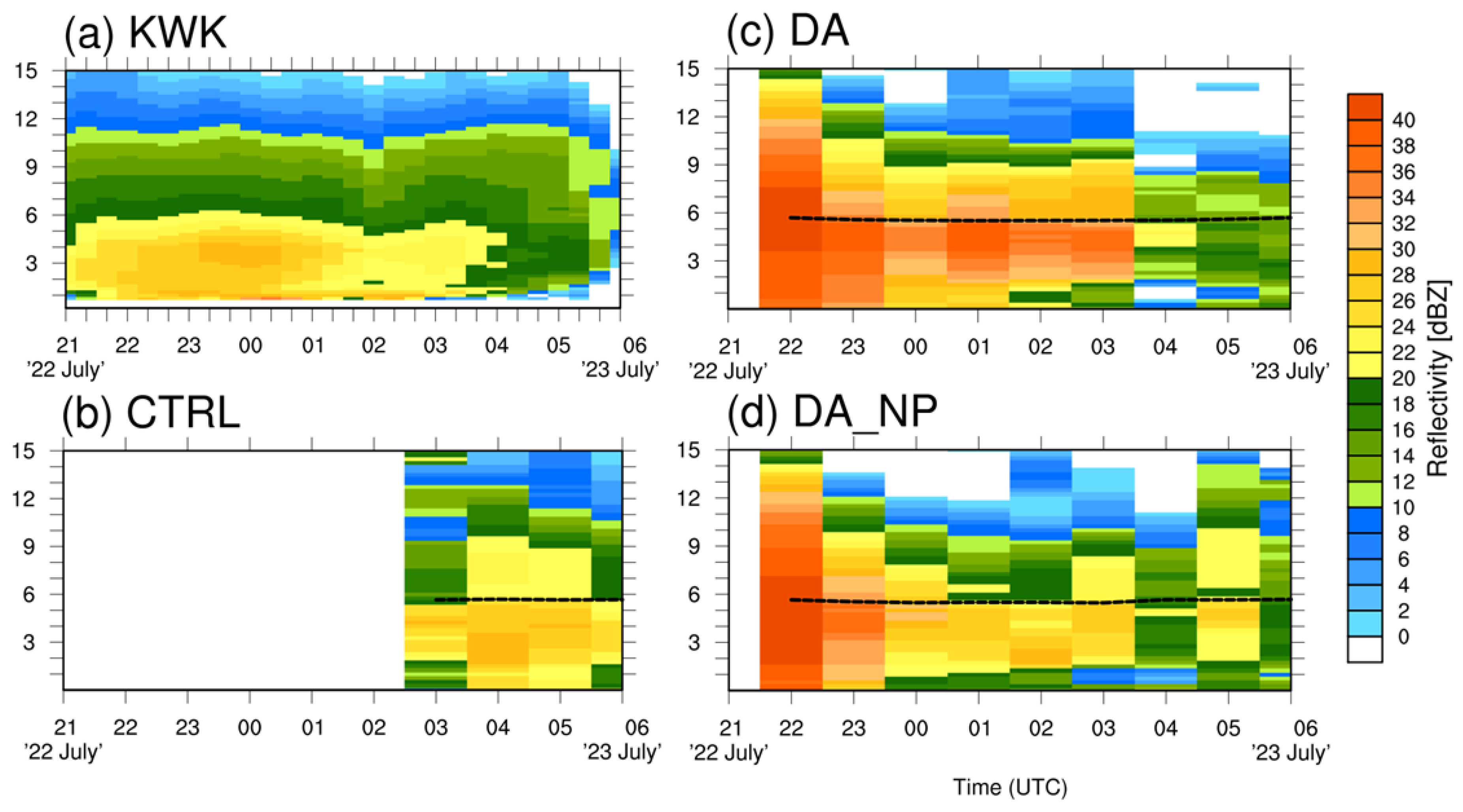
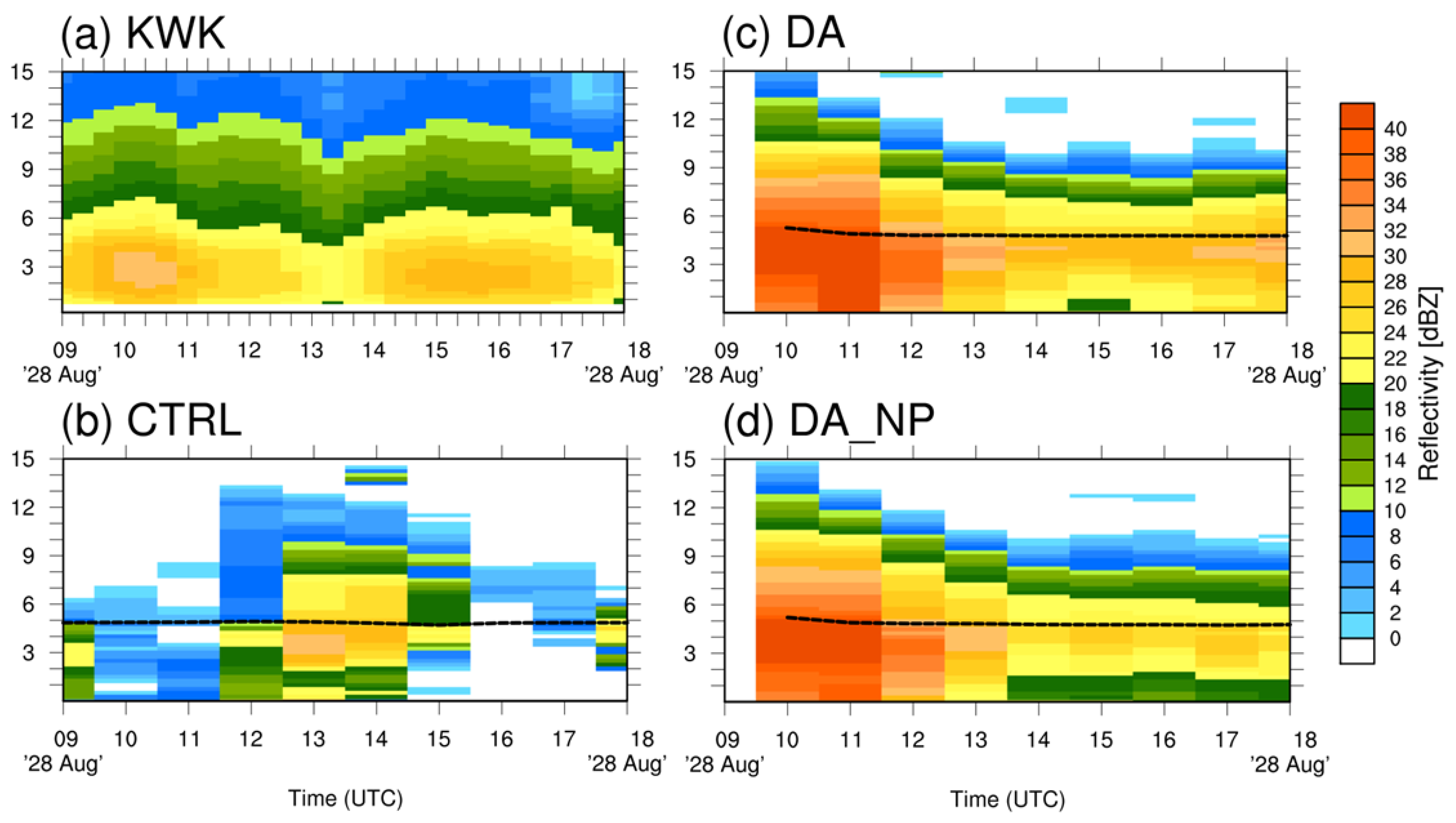
The characteristics and development of reflectivity (precipitation) over time were analyzed through THCSs. Figure 15 shows the THCSs of the KWK radar site and the CTRL, DA, and DA_NP experiments. Precipitation was observed in the KWK radar throughout the forecast period, with a reflectivity peak of about 30 dBZ near 4 km from 2230 UTC 22 July to 0030 UTC 23 July. In the CTRL, reflectivity was not found until 0300 UTC 23 July because precipitation was not simulated by the model. In the DA and DA_NP experiments, the THCSs were similar to that of the KWK reflectivity, but strong reflectivity occurred early in the prediction during the cycling period. The hydrometeors and humidity were added to existing moisture field of the model, and a larger amount of precipitation was simulated at the beginning of the prediction, simulating a precipitation peak from 2200 UTC to 2300 UTC 22 July. DA_NP showed the most similar reflectivity compared to KWK by reducing the over-simulated reflectivity through null-echo data assimilation. Null-echo data assimilation removed the excessive precipitation during the forecast period by removing the water vapor in the atmosphere, which reduced the mean reflectivity during the 2–6 h forecast period. However, it was not effective in controlling the strong reflectivity that occurred immediately after the cycling period from 2200 UTC to 2300 UTC 22 July. Figure 16 is the THCS of Case 3. Reflectivity was observed throughout the simulated period in KWK, but the CTRL only simulated the reflectivity in the beginning and middle of the period, with the amount less than that of KWK. DA and DA_NP overestimated the reflectivity but simulated the precipitation peak, similarly to the observations. DA_NP in Case 3 also showed lower reflectivity than DA, reducing the over-simulated precipitation from 1400 UTC to 1800 UTC 23 July.

4. Summary and Conclusions

This study investigated the ability of the high-resolution WRF model to simulate summer precipitation with dual polarized X-Net data over the Seoul metropolitan area. DA experiments with X-Net (S- and X-band Doppler radar) radial velocity and reflectivity data for convective summer monsoon events were evaluated. The conventional assimilation of radar data, which involved the assimilation of reflectivity and radial velocities from precipitation echoes, and the assimilation of null-echoes and its effects on short term QPF were studied. Three heavy rain events were simulated and analyzed in detail by comparing the cumulative precipitation, CFADs, THCSs, and verification statistics.

This study was conducted by using S- and X-band radar with AWS data. Radar reflectivity was firstly partitioned to corresponding hydrometeor types based on the background model temperature. The classified reflectivity was assimilated into the model by converting this value into a mixing ratio of four hydrometeors with the reflectivity mixing ratio relationship. The numerical experiment for the initial and boundary conditions without data assimilation, the CTRL, was used as a measure of the degree of improvement of radar data assimilation. The traditional radar data assimilation method, referred to as the DA experiment, only applied precipitation radar echoes in the assimilation. The DA_NP experiment assimilated both weather radar echoes and null-echoes to suppress and correct erroneous model precipitation.

The results of the horizontal incremental analysis showed that the water vapor mixing ratio and hydrometeors increased in areas where radar reflectivity was observed for both DA and DA_NP. In DA_NP, null-echo information was added, and the over-simulated water vapor and hydrometeors were removed. Accuracy evaluation with the total cumulative precipitation resulted in reduced errors for DA and DA_NP compared to the CTRL. However, over-predicted precipitation is a known problem when radar data are assimilated. DA_NP showed the highest accuracy by reducing over-simulated precipitation through null-echo data assimilation. This effect was also shown in the verification statistics, with the highest score from DA_NP up to 6 h when the effect of data assimilation was sustained. CFAD analysis was performed to analyze the microphysical structure of precipitation. The data assimilation simulated the process of hydrometeors falling and growing from the upper atmosphere. The CFADs also showed a decrease in reflectivity because of the reduction in over-predicted hydrometeors in DA_NP. The characteristics and development of reflectivity (precipitation) over time were also analyzed with THCSs. Although the precipitation peak was not simulated in the CTRL, strong reflectivity below the melting layer was simulated in DA and DA_NP, similarly to the observations at the peak precipitation times. Thus, precipitation predictability was improved through null-echo data assimilation. This study demonstrated the applicability of null-echo data assimilation to simulate convective storms when radar data assimilation is utilized. The application of this radar data assimilation method can increase the predictive accuracy.

When performing radar data assimilation, problems with over-simulating reflectivity in the model and causing heavy precipitation can be found early in the forecast period. Further study is needed to evaluate the detailed performance of how microphysics and convective schemes play a role in assimilation and reduce the dynamical imbalance from discontinuity that is generated by radar data assimilation.

References

- Korea Meteorological Society (KMS). Yealy KMA 2017 Wearther; KMA: Seoul, Korea, 2018; p. 10. [Google Scholar]
- Orlanski, I. A rational subdivision of scales for atmospheric processes. Bull. Am. Meteorol. Soc. 1975, 56, 527–530. [Google Scholar]
- Anthes, R.A.; Kuo, Y.H.; Baumhefner, D.P.; Errico, R.M.; Bettge, T.W. Predictability of Mesoscale Atmospheric Motions. Adv. Geophys. 1985, 28, 159–202. [Google Scholar]
- Lim, S.; Allabakash, S.; Chandrasekar, V.; Min, K.-H.; Choo, J.; Jang, B. X-Band Dual-Polarization Radar Observations of Snow Growth Processes of a Severe Winter Storm: Case of 12 December 2013 in South Korea. J. Atmos. Ocean. Technol. 2019, 36, 1217–1235. [Google Scholar] [CrossRef]
- Albers, S.C.; McGinley, J.A.; Birkenheuer, D.L.; Smart, J.R. The Local Analysis and Prediction System (LAPS): Analyses of Clouds, Precipitation, and Temperature. Weather Forecast. 1996, 11, 273–287. [Google Scholar] [CrossRef] [Green Version]
- Souto, M.J.; Balseiro, C.F.; Pérez-Muñuzuri, V.; Xue, M.; Brewster, K. Impact of Cloud Analysis on Numerical Weather Prediction in the Galician Region of Spain. J. Appl. Meteorol. 2003, 42, 129–140. [Google Scholar] [CrossRef] [Green Version]
- Gao, J.; Stensrud, D.J. Assimilation of reflectivity data in a convective-scale, cycled 3DVAR framework with hydrometeor classification. J. Atmos. Sci. 2012, 69, 1054–1065. [Google Scholar] [CrossRef]
- Wang, H.; Sun, J.; Fan, S.; Huang, X.-Y. Indirect assimilation of radar reflectivity with WRF 3D-Var and its impact on prediction of four summertime convective events. J. Appl. Meteorol. Climatol. 2013, 52, 889–902. [Google Scholar] [CrossRef]
- Gao, S.; Min, J.; Liu, L.; Ren, C. The development of a hybrid EnSRF-En3DVar system for convective-scale data assimilation. Atmos. Res. 2019, 229, 208–223. [Google Scholar] [CrossRef]
- Lee, Y.-H.; Min, K.-H. High-resolution modeling study of an isolated convective storm over Seoul Metropolitan area. Meteorol. Atmos. Phys. 2019, in press. [Google Scholar] [CrossRef]
- Abhilash, S.; Sahai, A.; Mohankumar, K.; George, J.P.; Das, S. Assimilation of Doppler weather radar radial velocity and reflectivity observations in WRF-3DVAR system for short-range forecasting of convective storms. Pure Appl. Geophys. 2012, 169, 2047–2070. [Google Scholar] [CrossRef]
- Bachmann, K.; Keil, C.; Craig, G.; Weissmann, M.; Welzbacher, C. Predictability of deep convection in idealized and operational forecasts: Effects of radar data assimilation, orography and synoptic weather regime. Mon. Weather Rev. 2019, in press. [Google Scholar] [CrossRef]
- Gao, J.; Fu, C.; Kain, J.; Stensrud, D.J. OSSEs for an ensemble 3DVAR data assimilation system with radar observations of convective storms. J. Atmos. Sci. 2016, 73, 2403–2426. [Google Scholar] [CrossRef]
- Hu, M.; Xue, M.; Gao, J.; Brewster, K. 3DVAR and Cloud Analysis with WSR-88D Level-II Data for the Prediction of the Fort Worth, Texas, Tornadic Thunderstorms. Part II: Impact of Radial Velocity Analysis via 3DVAR. Mon. Weather Rev. 2006, 134, 699–721. [Google Scholar] [CrossRef]
- Sugimoto, S.; Crook, N.A.; Sun, J.; Xiao, Q.; Barker, D.M. An examination of WRF 3DVAR radar data assimilation on its capability in retrieving unobserved variables and forecasting precipitation through observing system simulation experiments. Mon. Weather Rev. 2009, 137, 4011–4029. [Google Scholar] [CrossRef]
- Sun, J.; Wang, H. Radar Data Assimilation with WRF 4D-Var. Part II: Comparison with 3D-Var for a Squall Line over the U.S. Great Plains. Mon. Weather Rev. 2013, 141, 2245–2264. [Google Scholar] [CrossRef]
- Xiao, Q.; Sun, J. Multiple-radar data assimilation and short-range quantitative precipitation forecasting of a squall line observed during IHOP_2002. Mon. Weather Rev. 2007, 135, 3381–3404. [Google Scholar] [CrossRef]
- Xiao, Q.; Kuo, Y.-H.; Sun, J.; Lee, W.-C.; Barker, D.M.; Lim, E. An approach of radar reflectivity data assimilation and its assessment with the inland QPF of Typhoon Rusa (2002) at landfall. J. Appl. Meteorol. Climatol. 2007, 46, 14–22. [Google Scholar] [CrossRef] [Green Version]
- Wattrelot, E.; Caumont, O.; Mahfouf, J.-F. Operational Implementation of the 1D+3D-Var Assimilation Method of Radar Reflectivity Data in the AROME Model. Mon. Weather Rev. 2014, 142, 1852–1873. [Google Scholar] [CrossRef] [Green Version]
- Min, K.-H.; Kim, Y.-H. Assimilation of null-echo from radar data for QPF. In Proceedings of the 17th WRF Users’ Workshop, Boulder, CO, USA, 27 June–1 July 2016. [Google Scholar]
- Gao, S.; Sun, J.; Min, J.; Zhang, Y.; Ying, Z. A scheme to assimilate “no rain” observations from Doppler radar. Weather Forecast. 2018, 33, 71–88. [Google Scholar] [CrossRef]
- Xiao, Q.; Kuo, Y.-H.; Sun, J.; Lee, W.-C.; Lim, E.; Guo, Y.-R.; Barker, D.M. Assimilation of Doppler radar observations with a regional 3DVAR system: Impact of Doppler velocities on forecasts of a heavy rainfall case. J. Appl. Meteorol. 2005, 44, 768–788. [Google Scholar] [CrossRef]
- Ye, B.-Y.; Lee, G.; Park, H.-M. Identification and removal of non-meteorological echoes in dual-polarization radar data based on a fuzzy logic algorithm. Adv. Atmos. Sci. 2015, 32, 1217–1230. [Google Scholar] [CrossRef]
- Barker, D.M.; Huang, W.; Guo, Y.-R.; Bourgeois, A.J.; Xiao, Q.N. A three-dimensional variational data assimilation system for MM5: Implementation and initial results. Mon. Weather Rev. 2004, 132, 897–914. [Google Scholar] [CrossRef] [Green Version]
- Barker, D.M.; Coauthors. The Weather Research and Forecasting (WRF) Model’s Community Variational/Ensemble Data Assimilation System: WRFDA. Bull. Am. Meteorol. Soc. 2012, 93, 831–843. [Google Scholar] [CrossRef] [Green Version]
- Parrish, D.F.; Derber, J.C. The National Meteorological Center’s spectral statistical-interpolation analysis system. Mon. Weather Rev. 1992, 120, 1747–1763. [Google Scholar] [CrossRef]
- Lin, Y.; Farley, R.D.; Orville, H.D. Bulk paramete-rization of the snow field in a cloud model. J. Clim. Appl. Meteorol. 1983, 22, 1065–1092. [Google Scholar] [CrossRef] [Green Version]
- Gilmore, M.S.; Wicker, L.J. The influence of mid-tropospheric dryness on supercell morphology and evo-lution. Mon. Weather Rev. 1998, 126, 943–958. [Google Scholar] [CrossRef]
- Dowell, D.C.; Wicker, L.J.; Snyder, C. Ensemble Kalman filter assimilation of radar observations of the 8 May 2003 Oklahoma City supercell: Influences of refl-ectivity observations on storm-scale analyses. Mon. Weather Rev. 2011, 139, 272–294. [Google Scholar] [CrossRef] [Green Version]
- Smith, P.L., Jr.; Myers, C.G.; Orville, H.D. Radar reflectivity factor calculations in numerical cloud models using bulk parameterization of precipitation processes. J. Appl. Meteorol. 1975, 14, 1156–1165. [Google Scholar] [CrossRef] [Green Version]
- Sun, J.; Crook, N.A. Dynamical and microphysical retrieval from Doppler radar observations using a cloud model and its adjoint. Part I: Model development and simulated data experiments. J. Atmos. Sci. 1997, 54, 1642–1661. [Google Scholar] [CrossRef]
- Skamarock, W.C.; Klemp, J.B.; Dudhia, J.; Gill, D.O.; Barker, D.M.; Wang, W.; Powers, J.G. A Description of the Advanced Research WRF Version 2. NCAR Tech. Note NCAR/TN-4681STR; UCAR Communications: Boulder, CO, USA, 2008; 88p. [Google Scholar] [CrossRef] [Green Version]
- Zheng, Y.; Alapaty, K.; Herwehe, J.S.; Del Genio, A.; Niyogi, D. Improving high-resolution weather forecasts using the Weather Research and Forecasting (WRF) Model with an updated Kain–Fritsch scheme. Mon. Weather Rev. 2016, 144, 833–860. [Google Scholar] [CrossRef]
- Lim, K.-S.S.; Hong, S.-Y. Development of an effective double-moment cloud microphysics scheme with prognostic cloud condensation nuclei (CCN) for weather and climate models. Mon. Weather Rev. 2010, 138, 1587–1612. [Google Scholar] [CrossRef] [Green Version]
- Hong, S.-Y.; Noh, Y.; Dudhia, J. A new vertical diffusion package with an explicit treatment of entrainm-ent processes. Mon. Weather Rev. 2006, 134, 2318–2341. [Google Scholar] [CrossRef] [Green Version]
- Mlawer, E.J.; Taubman, S.J.; Brown, P.D.; Iacono, M.J.; Clough, S.A. Radiative transfer for inhomogeneous atmospheres: RRTM, a validated correlated-k model for the longwave. J. Geophys. Res. 1997, 102, 16663–16682. [Google Scholar] [CrossRef] [Green Version]
- Dudhia, J. Numerical study of convection observed during the Winter Monsoon Experiment using a mesosca-le two-dimensional model. J. Atmos. Sci. 1989, 46, 3077–3107. [Google Scholar] [CrossRef]
- Jimenez, P.A.; Dudhia, J.; Gonzalez-Rouco, J.F.; Navarro, J.; Montavez, J.P.; Garcia-Bustamante, E. A revi-sed scheme for the WRF surface layer formulation. Mon. Weather Rev. 2012, 140, 898–918. [Google Scholar] [CrossRef] [Green Version]
- Tewari, M.; Chen, F.; Wang, W.; Dudhia, J.; LeMone, M.A.; Mitchell, K.; Ek, M.; Gayno, G.; Wegiel, J.; Cuenca, R.H. Implementation and verification of the unified Noah land-surface model in the WRF Model. In Proceedings of the 20th Conference on Weather Analysis and Forecasting, Seattle, WA, USA, 10–15 January 2004; p. 14.2a. [Google Scholar]
- Yuter, S.E.; Houze, R.A. Three-dimensional kinematic and microphysical evolution of Florida cumulonimbus. Part II: Frequency distributions of vertical velocity, reflectivity, and differential reflectivity. Mon. Weather Rev. 1995, 123, 1941–1963. [Google Scholar] [CrossRef]
- Wang, J.-J.; Carey, L. The Development and Structure of an Oceanic Squall-Line System during the South China Sea Monsoon Experiment. Mon. Weather Rev. 2005, 133, 1544–1561. [Google Scholar] [CrossRef]
- Min, K.-H.; Choo, S.-H.; Lee, D.-H.; Lee, G.-W. Evaluation of WRF Cloud Microphysics Schemes Using Radar Observations. Weather Forecast. 2015, 30, 1571–1589. [Google Scholar] [CrossRef]
- Cecil, D.J. Relating passive 37-GHz scattering to radar profiles in strong convection. J. Appl. Meteorol. Climatol. 2011, 50, 233–240. [Google Scholar] [CrossRef]
Figure 1.
Locations of the S-band radars (blue dots), X-band radars (red dots), automated weather station (AWS) sites (gray dots), and radiosondes (yellow dots), with the radar coverage areas in circles.
Figure 2.
Flow chart for assimilating radar reflectivity with null-echo observation operators.
Figure 3.
(a) Domain configuration and topography (shaded) of D01, D02, and D03; (b) the border lines of city and provinces used in D03 (the borders are shown as a red line for Seoul, an orange line for Gyeonggi, and a blue line for Hwanghae).
Figure 4.
Synoptic analysis for (a) 0000 UTC 2 July 2017, (b) 1200 UTC 22 July 2017, and (c) 0000 UTC 28 August 2018.
Figure 5.
Comparison of (a) the radar reflectivity (dBZ), reflectivity of (b) CTRL, (c) DA, and (d) DA_NP and the difference in qv between (e) DA and CTRL and between (f) DA_NP and CTRL at 0900 UTC 2 July 2017.
Figure 6.
Same as Figure 5 except for 2100 UTC 22 July 2017.
Figure 7.
Same as Figure 5 except for 0900 UTC 28 August 2018.
Figure 8.
Cumulative precipitation (mm) distribution for Case 1 from the (a) AWSs, (b) CTRL, (c) DA, and (d) DA_NP at D03.
Figure 9.
Same as Figure 8 except for Case 2.
Figure 10.
Same as Figure 8 except for Case 3.
Figure 11.
Verification statistics of the (a) accuracy, (b) critical success index (CSI), and (c) equitable threat score (ETS) for CTRL (black lines), DA (red lines), and DA_NP (blue lines).
Figure 12.
Vertical profiles biases of (a) water vapor mixing ratio, (b) temperature, (c) U wind component, and (d) V wind component for CTRL (black lines), DA (red lines), and DA_NP (blue lines) at 2017.07.02.1200 UTC (solid lines) and 2018.08.28.1200 UTC (dashed lines).
Figure 13.
Contoured frequency by altitude diagram (CFAD) percentiles of the (a) Kwanak Mountain Mountain (KWK) observed and (b) CTRL, (c) DA, and (d) DA_NP simulated radar reflectivity for Case 2. The horizontal black dotted line in each panel represents the model’s 0 °C height (b, c, and d). The cumulative reflectivity frequencies of the 25th, 50th, and 75th percentiles are marked with black solid lines, the average reflectivity factor in linear units (mm−6·m−3) is marked by a white solid line, and the average reflectivity is marked by a red solid line (KWK) and blue solid line (models).
Figure 14.
Same as Figure 13 except for Case 3 forecast period.
Figure 15.
Time–height cross-sections for Case 2 at the KWK radar site for (a) the observations, (b) CTRL, (c) DA, and (d) DA_NP.
Figure 16.
Same as Figure 15 except for Case 3 forecast period.