PolSAR Image Classification Based on Statistical Distribution and MRF

Abstract

Classification is an important topic in synthetic aperture radar (SAR) image processing and interpretation. Because of speckle and imaging geometrical distortions, land cover mapping is always a challenging task especially in complex landscapes. In this study, we aim to find a robust and efficient method for polarimetric SAR (PolSAR) image classification. The Markov random field (MRF) has been widely used for capturing the spatial-contextual information of the image. In this paper, we firstly introduce two ways to construct the Wishart mixture model and compare their performances using real PolSAR data. Then, the better mixture model and two other classical statistically distributions are combined with MRF to construct the MRF models. In order to improve the robustness of the models, the constant false alarm rate (CFAR)-based edge penalty term and an adaptive neighborhood system are embedded into the MRF energy functional. Classification is implemented in two schemes, i.e., pixel-based and region-based classifications. Finally, agriculture fields are used as the test scenario to evaluate the robustness and applicability of these algorithms.

1. Introduction

Due to the all-weather and all-day high-resolution imaging capability, synthetic aperture radar (SAR) is widely favored in the field of remote sensing and has become an indispensable and important branch of remote sensing information acquisition technology. The SAR system acquires the scattering characteristics of ground targets in a specific transmitting and receiving polarization, which is a single channel system. Polarimetric SAR (PolSAR) offers multichannel information, and the fully or quad polarimetric SAR systems allow the complete backscattering characterization of scatterers [1,2]. Polarimetric information greatly improves the application capabilities of satellite SAR systems [3,4]. Classification is an important step in image analysis and interpretation, which is also a research hotspot in many applications. However, polarimetric SAR data acquired from different terrain types have different statistics, which causes difficulties in PolSAR image classification.

In 1988, Kong J A et al. [5] developed a systematic approach for PolSAR image classification. They proposed that land cover classification aims to assign pixels into different classes. Since then, many researchers continued the research, and many classification algorithms have been proposed. According to the different features used, polarimetric SAR image classification methods can be summarized into two categories: classification based on statistical properties and classification based on polarization scattering mechanisms [6,7]. The classification based on statistical properties is derived from the statistical models of PolSAR data. Statistical properties have an indispensable effect on classification tasks. In 1994, Lee J S et al. [8] proposed the Wishart distribution-based maximum likelihood (ML) classifier, which is the most widely used statistical model-based method for PolSAR images. However, this distribution only applies well to homogeneous regions. For the textural regions, the product models were developed. The earliest study of the product model was the K distribution proposed by Jao J [9]. Then, Lee J S et al. [10] proved that multi-look PolSAR data also obey the K distribution. In 2005, Freitas C C et al. [11] proposed the G-distribution, which has a better description for the heterogeneous regions. In addition to using a single distribution model for the heterogenous areas, many mixture models have also been proposed [12], in which the Wishart mixture model is a widely used and effective finite mixture model for PolSAR data [13,14]. The superiority of mixture models has been verified by many studies [12,13,14,15]. However, these methods do not consider the spatial information of the image.

The Markov random field (MRF) [16] is a representative algorithm framework that can fully consider spatial contextual information. MRF has long been used for both optic and SAR image classification. In 1995, Yamazaki et al. [17] developed a hierarchical Markov random field (MRF) model that consisted of the observed intensity process and the hidden class label process for remote sensing images and textured images. Deng H et al. [18] developed an anisotropic circular Gaussian MRF (ACGMRF) model for image classification. This model has proven to have statistical improvement. Dong Y et al. [19] first applied MRF to PolSAR image classification. Then, Wu et al. [20] combined the region-based over-segmentation with MRF to implement the PolSAR image classification. For the limitations of the auxiliary label field, Liu et al. [21] proposed the triple Markov field (TMF) and its improved model for PolSAR data. Shi J et al. [22] proposed an adaptive MRF framework based on a polarimetric sketch map, which can preserve image details. In 2016, Masjedi A et al. [23] related the Markovian energy-difference function to the SVM classifier. It has been proven that the speckle effect on the classified map is greatly reduced when using the contextual classifier. Li et al. [24] proposed a Gaussian mixture model (GMM)-MRF method, which combines GMM with the spatial-contextual information of images modeled by MRF, where the GMM serves as a likelihood classifier in the MRF framework. Song et al. [25] proposed a mixture WGΓ-MRF (MWGΓ-MRF) model for PolSAR image classification. By introducing the MRF model into each component of the WGΓMM model, the spatial-contextual information of images can be better captured.

In this study, we focus on the MRF-based models for PolSAR image classification. The Wishart, K-Wishart, and mixture distributions are considered, and the mixture strategies are compared. In order to improve the robustness and effectiveness of the method, we employ the adaptive neighborhood system in the MRF model, as well as the edge penalty term used to locate the image edges accurately. Finally, the MRF-based methods are implemented in both pixel-based and region-based classifications.

The remainder of this study is organized as follows. Section 2 introduces the statistical models and the MRF model. In Section 3, we introduce two classification schemes, which are the pixel-based classification and the region-based classification. In Section 4, classification is performed and evaluated on data of agricultural field areas. We conclude this study in Section 5.

2. MRF-Based Classification Models

2.1. Statistical Models

Statistical modeling is a key problem in random field models. Constructing an accurate statistical distribution has been the research focus in the field of polarimetric SAR image processing. Many statistical models have been proposed for polarimetric SAR data, in which the Wishart distribution is an efficient and widely used model.

For homogeneous regions in multi-look PolSAR images, the polarimetric covariance matrix $\mathit{C}=\left\{{\mathit{C}}_1,{\mathit{C}}_2,\dots {\mathit{C}}_{\mathit{N}}\right\}$ obeys the Wishart distribution [26],

$$P^W\left({\mathit{C}}_i\right)=\frac{L^{Lq}{\left|{\mathit{C}}_i\right|}^{L-q}\exp \left\{-LTr\left({\mathbf{\Sigma }}^{-1}{\mathit{C}}_i\right)\right\}}{R\left(L,q\right){\left|\mathbf{\Sigma }\right|}^L},$$

(1)

where $Tr(·)$ stands for trace of a matrix, L denotes the number of looks, q is the number of channels, and $\mathbf{\Sigma }$ is the mean covariance matrix. $R\left(L,q\right)={\pi }^{q\left(q-1\right)/2}\mathsf{\Gamma }\left(L\right)\dots \mathsf{\Gamma }\left(L-q+1\right)$ is the scaling function with a Gamma function $\mathsf{\Gamma }(\cdot )$.

The complex Wishart distribution is simple and easy to calculate. In 1994, Lee J S et al. [10] used the Gamma distribution to derive the K distribution for the covariance matrix and then combined it with the Wishart distribution to derive the K-Wishart distribution. The K-Wishart distribution is better at modeling textural areas, which combines the Gamma distribution as the texture component and the Wishart distribution as the speckle component,

$$P^K\left({\mathit{C}}_i\right)=\frac{2{\left|{\mathit{C}}_i\right|}^{L-q}}{R\left(L,q\right)\mathsf{\Gamma }\left(\sigma \right){\left|\mathbf{\Sigma }\right|}^L}{\left(L\sigma \right)}^{\frac{q+Lq}{2}}\cdot {\left(Tr\left({\mathbf{\Sigma }}^{-1}{\mathit{C}}_i\right)\right)}^{\frac{\sigma -Lq}{2}}{K}_{\sigma -Lq}\left(2\sqrt{L\sigma Tr\left({\mathbf{\Sigma }}^{-1}{\mathit{C}}_i\right)}\right),$$

(2)

where $K_{\rho }(\cdot )$ is the second modified Bessel function with order ρ and α is the shape parameter. The K-Wishart distribution is not only suitable for describing homogeneous areas, but also applied well for heterogeneous areas, for which the probability distribution is not fitted well by the complex Wishart distribution. It has a better fitting agreement with the real data even for the extremely heterogeneous regions.

2.2. Mixture Strategies

Sometimes, the data we are trying to model are complex, in which case the mixture distribution is usually used. Mixture models can better describe heterogeneous regions in polarimetric SAR images. The Wishart distribution is widely used to model the fully developed speckle. For areas with less developed speckle, we use a mixture of Wishart distributions to fit the statistics. In this section, we consider two strategies to form the mixture models. One is to model the whole image by using a Wishart mixture model, and the other is to model a class by using a Wishart mixture model. Real data are used to evaluate the performance of mixture strategies. Then, the better mixture strategy will be combined with MRF to develop the spatial-contextual classifier.

2.2.1. Mixture Wishart for a Whole Image

The finite mixture model [12] was proposed to consider the polarimetric information and the spatial context fully. Compared to the traditional Wishart distribution, a mixture of Wishart models can better model the heterogeneous regions [12,13,14,15,27].

Each component of the mixture model corresponds to a specific cluster. Then, the number of components equals the number of classes, i.e.,

$$\begin{array}{ll}{P}_M^W\left({\mathit{C}}_i\right)& ={\displaystyle \sum _{k=1}^K{\pi }_k{p}^W\left({\mathit{C}}_i\right)}\\ & ={\displaystyle \sum _{k=1}^K{\pi }_k\frac{L^{Lq}{\left|{\mathit{C}}_i\right|}^{L-q}\exp \left\{-LTr\left({\mathbf{\Sigma }}_k^{-1}{\mathit{C}}_i\right)\right\}}{R\left(L,q\right){\left|{\mathbf{\Sigma }}_k\right|}^L}}\end{array}$$

(3)

where ${\mathbf{\Sigma }}_{\mathit{k}},k=1,2,\dots ,K$ is the mean covariance matrix of each cluster. ${\pi }_k$ is the weight of each component, which should satisfy ${\displaystyle \sum _{k=1}^K{\pi }_k}=1$ and ${\pi }_k\ge 0$. The expectation-maximization (EM) algorithm is adopted to update the variables ${\mathbf{\Sigma }}_{\mathit{k}}$ and ${\pi }_k$. According to the EM algorithm, the parameters can be estimated by maximizing the log-likelihood function as follows:

$${\Sigma }_k=\frac{{\displaystyle {\sum }_{i=1}^N\frac{{\pi }_k{p}^W\left({\mathit{C}}_i\right)}{{\displaystyle {\sum }_{k=1}^K{\pi }_k{p}^W\left({\mathit{C}}_i\right)}}{\mathit{C}}_i}}{{\displaystyle {\sum }_{i=1}^N\frac{{\pi }_k{p}^W\left({\mathit{C}}_i\right)}{{\displaystyle {\sum }_{k=1}^K{\pi }_k{p}^W\left({\mathit{C}}_i\right)}}}},$$

(4)

$${\pi }_k=\frac{1}{N}{\displaystyle \sum _{n=1}^N\frac{{\pi }_k{p}^W\left({\mathit{C}}_i\right)}{{\displaystyle {\sum }_{k=1}^K{\pi }_k{p}^W\left({\mathit{C}}_i\right)}}},$$

(5)

where N is the number of pixels of the whole image.

2.2.2. Mixture Wishart for a Class

The method mentioned above is to model the whole image by using a mixture model, with each mixture component corresponding to a cluster. Therefore, each class is essentially described by a single component distribution. Gao W [14] proposed another way to form the mixture distribution, which uses a set of components to present the distribution density for a single class. For class k, the Wishart mixture distribution is generated by M Wishart components,

$$\begin{array}{ll}{P}_M^W\left({\mathit{C}}_i\right)& ={\displaystyle \sum _{m=1}^M{\pi }_m^k{p}^W\left({\mathit{C}}_i\right)}\\ & ={\displaystyle \sum _{m=1}^M{\pi }_m^k\frac{L^{Lq}{\left|{\mathit{C}}_i\right|}^{L-q}\exp \left\{-nTr\left({\mathbf{\Sigma }}_m^k\backslash {\mathit{C}}_i\right)\right\}}{R\left(L,q\right){\left|{\mathbf{\Sigma }}_m^k\right|}^n}}\end{array}$$

(6)

where ${\mathbf{\Sigma }}_m^k,m=1,2,\dots ,M$ denotes the centroids of each Wishart component for class k. Each component is associated with a weight ${\pi }_m^k$, which should satisfy ${\displaystyle \sum _{m=1}^M{\pi }_m^k}=1$ and ${\pi }_m^k\ge 0$. The EM algorithm is employed to determine the mixture model parameters for the mixture Wishart for a class (MWC) strategy. Classification is based on the maximum likelihood criterion.

The number of mixed components M is difficult to determine. Theoretically, the overall accuracy of classification improves when the number of mixture components increases, but the cost of computation also increases. In this study, to consider the trade-off between the computational burden and classification accuracy, the value was set to six. For each class, the centroids are firstly initialized by randomly selecting ${\mathit{C}}_{m_{\mathbf{i}}}$ from training samples, and ${\pi }_m^k$ are initialized as ${\pi }_m^k=1/M$. Then, these parameters are iteratively updated by the EM algorithm. After that, the distribution of each class can be expressed by the weighted sum of the Wishart components. The classifier labels a test sample with the class that has the largest likelihood value.

2.2.3. Comparison of the Two Mixture Strategies

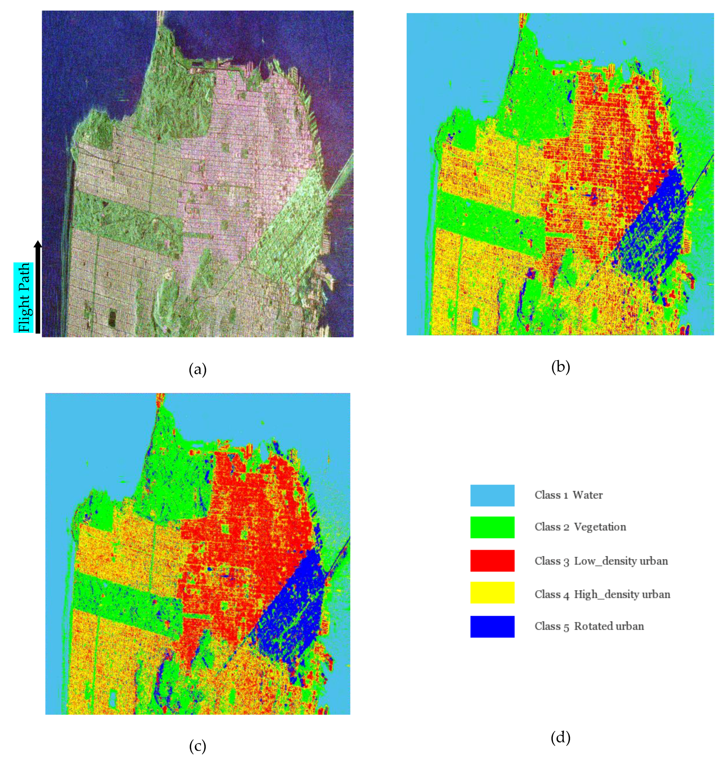
In order to compare which model is better to present the multi-look fully polarimetric SAR data, RADARSAT-2 data acquired over the San Francisco Bay area, USA, were used to evaluate the performance of the two mixture strategies. The Pauli color-coded image is shown in Figure 1a. The PolSAR image was filtered using the refined Lee filter with a 9 × 9 window.

The classification steps for the mixture Wishart for a whole image (MWW) algorithm are as follows:

• Initialize parameter ${\mathbf{\Sigma }}_k$ by randomly selecting one covariance matrix from each class of the image. ${\pi }_k$ is initialized as 1/K.
• Compute posterior probabilities using ${\mathbf{\Sigma }}_k$ and ${\pi }_k$, then update the class labels based on the maximum a posteriori decision rule.
• Update ${\mathbf{\Sigma }}_{\mathit{k}}$ and ${\pi }_k$ using (4) and (5).
• Check if the classification result has converged. If not, go back to Step 2. Otherwise, the iteration ends.

The classification steps of the MWC algorithm are different from those of MWW. For the MWW algorithm, it is the EM algorithm that performs the classification. MWC only uses the EM algorithm to estimate the parameters for each class, and the classification is based on the ML criterion. The classification steps are as follows:

• Randomly select m covariance matrices from the training samples of each class as the initialization of ${\mathbf{\Sigma }}_m^k$. ${\pi }_m^k$ is initialized as 1/M.
• Update the parameters using (4) and (5). Note that in MWC, the parameter N denotes the number of training samples of each class.
• Construct the mixture model for each class.
• Classify the image based on the ML criterion.

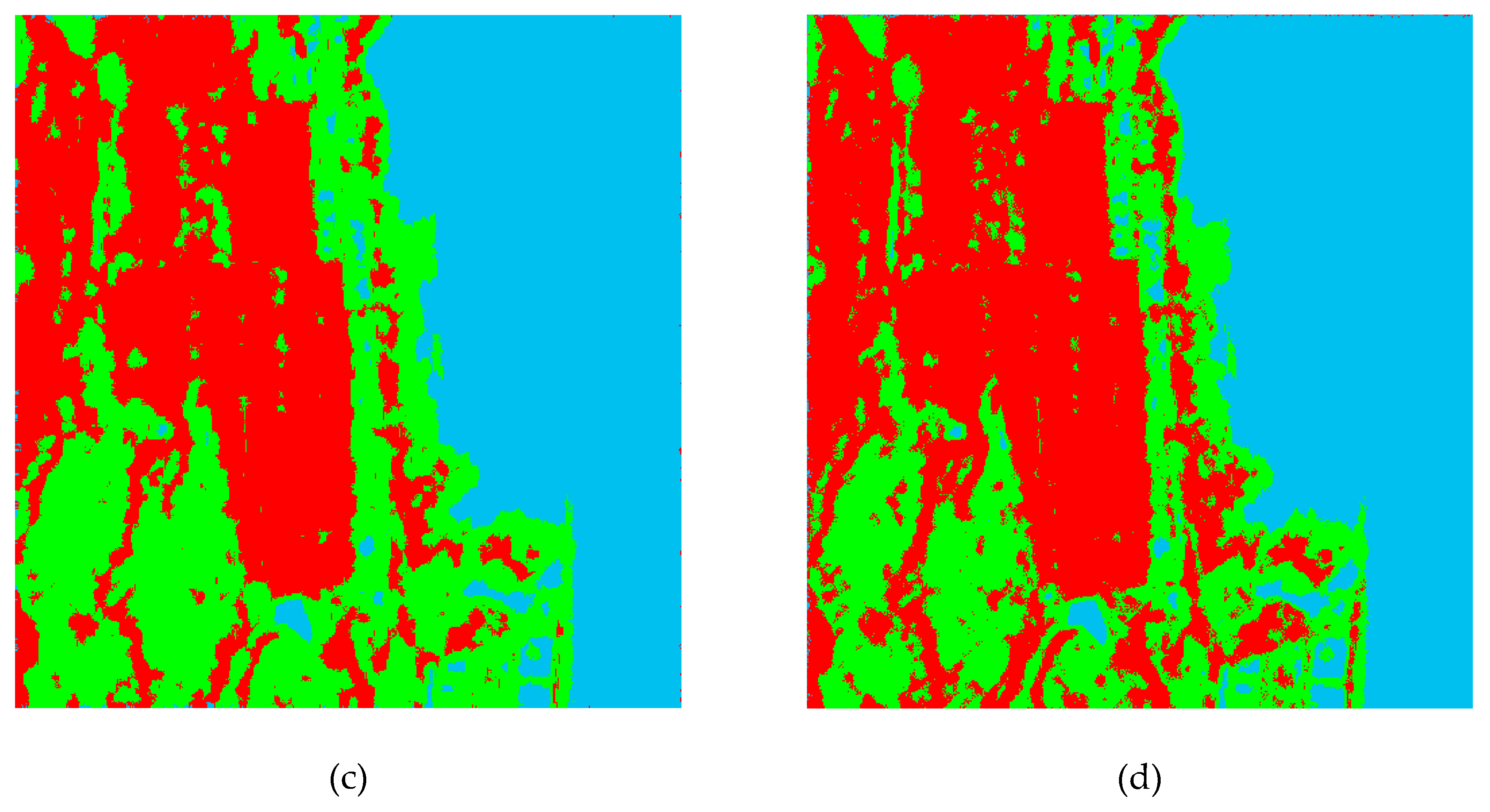
From Figure 1b,c, we can see that compared with MWW, the classification map of MWC was better by visual inspection, especially for water and urban areas. We can see from the classification results that on the right side of the image, the MWW model was affected greatly by the strong backscatter of the offshore buildings, resulting in misclassification. According to the exiting literature, we divided urban areas into three classes, which were low density urban, high density urban, and rotated urban. The MWC model could differentiate among the three types of urban areas better than the MWW model. The classification result of the rotated urban area based on the MWC model was relatively complete. Experiment results showed that using a mixture distribution to model a single class was more precise and could improve the land cover classification accuracy.

2.3. MRF-Based Classification Model

2.3.1. MRF

The Markov random field theory provides a convenient and consistent way of modeling context-dependent entities such as image pixels and correlated features.

Let S denote an image on a 2D lattice,

$$S=\left\{s_{xy},1\le x\le m,1\le y\le n\right\},$$

(7)

where $s_{xy}$ is the value for site $\left(x,y\right)$ and m and n are the number of rows and columns of the image. We assume that $X=\left\{x_i,i\in S\right\}$ is a random field defined on S. We call X an MRF with respect to a neighborhood system ${\eta }_i$, if and only if the following two conditions are satisfied:

$$\begin{array}{l}p\left(x_i\right)>0\left(\mathrm{positivity}\right)\\ p\left(x_i|x_{S\backslash i}\right)=p\left(x_i|x_{{\eta }_i}\right)\left(\mathrm{Markovianity}\right)\end{array},$$

(8)

where S\i is the set containing all sites in S except i. The Markovianity implies site i in S is related to its neighborhood system. Hammersley and Clifford [28] proved the equivalence between Markov random fields and Gibbs distributions, which provides a mathematically tractable means of specifying the joint probability of an MRF. A Gibbs distribution takes the form:

$$P\left(x\right)=\frac{1}{Z}\exp \left(-\frac{1}{T}U\left(x\right)\right),$$

(9)

where T is the shape parameter. In practice, T is usually taken as a constant. Let T = 1. Then, $Z={\displaystyle {\sum }_{x_i=1}^K\exp \left\{-U\left(x_i\right)\right\}}$ is a normalization coefficient. $U\left(x\right)={\displaystyle {\sum }_{C\in \xi }{V}_c\left(x\right)}$ is an energy function. C is a clique. ξ denotes all the cliques of η. $V_c\left(x\right)$ is a potential function. The energy function is defined as:

$$U\left(x_i\right)=-\beta {\displaystyle {\sum }_{j\in {\eta }_i}^{}\delta \left(x_i-x_j\right)},$$

(10)

where β>0 is a spatial smoothness parameter, and it encourages neighboring pixels to have the same region label. According to [29], we set the value of β to 1.4 in all our experiments. $\delta (\cdot )$ is the Delta function.

2.3.2. Adaptive Neighborhood System

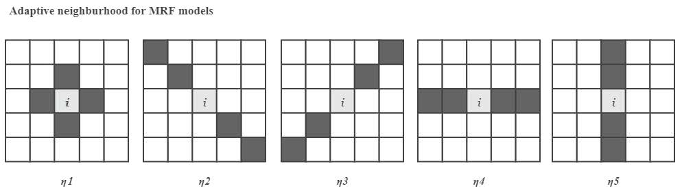
MRF takes advantage of the spatial information, so that the noise effect in the classification can be alleviated. A fixed neighborhood could result in blurred-structure details. In order to solve this problem, the adaptive neighborhood [30] is proposed to preserve the details of the image. The neighborhood system has five candidates, i.e., $\mathbf{\eta }=\left\{{\eta }_1,\dots ,{\eta }_5\right\}$, as shown in Figure 2. Each shape of the five candidates is related to a different terrain situation. The most suitable candidate is selected by the following criterion,

$$\eta =\arg \underset{i\in \left\{1,2,\dots ,5\right\}}{\min }\mathrm{std}\left(span({\eta }_i)\right),$$

(11)

where $span(\cdot )$ denotes the span values of pixels in ${\eta }_i$ and $\mathrm{std}(\cdot )$ denotes the standard deviation. By this means, the MRF model is better to fit the real terrain backscatter.

2.3.3. Edge Penalty

Though the adaptive MRF can preserve the structure details of the image, it cannot identify accurate edge locations. For PolSAR images with weak edges, MRF-based methods may cause misclassification [31,32]. In order to improve the classification robustness, we introduce an edge penalty term into the MRF model.

The CFAR edge detector [33] is used to calculate the edges, which was proposed by Schou J in 2003. The edge detection is performed pixel-by-pixel. For each pixel, a set of filters that have different orientations is applied. The filters estimate the mean covariance matrices of the two sides of the filter window for the central pixel and test the equality of these two mean covariance matrices using the Wishart likelihood-ratio as follows:

$$Q=\frac{{\left(L_x+L_y\right)}^{q\left(L_x+L_y\right)}}{L_x{}^{q{L}_x}{L}_y{}^{p{L}_y}}\frac{{\left|{\mathit{Z}}_x\right|}^{L_x}{\left|{\mathit{Z}}_y\right|}^{L_y}}{{\left|{\mathit{Z}}_x+{\mathit{Z}}_y\right|}^{L_x+L_y}},$$

(12)

where ${\mathit{Z}}_x$ and ${\mathit{Z}}_y$ are the mean covariance matrices on each side of the central pixel and $L_x$ and $L_y$ are the number of looks. Suppose the minimum $Q$ of all filters is $Q_{\min }$. Then, $-2\rho \log Q_{\min }$ is defined as the strength of the edge. If $-2\rho \log Q_{\min }$ is larger than a threshold, an edge is detected. The parameter ρ is:

$$\rho =1-\frac{2q^2-1}{6q}\left(\frac{1}{L_x}+\frac{1}{L_y}-\frac{1}{L_x+L_y}\right).$$

(13)

After extracting the edge information, the edge penalty function $g\left(e_i,e_j\right)$ [18] is constructed, as follows:

$$g\left(e_i,e_j\right)=\exp \left\{\frac{-{\left(e_i-e_j\right)}^2}{edge\_c^2}\right\},$$

(14)

where $e_i$ is the edge strength of the site i and $edge\_c$ is a constant, which is used to balance the spatial-contextual information and the edge intensity. Adding this edge penalty term into the MRF energy function in (10), we get:

$$U_{edge}\left(x_i\right)=-\beta {\displaystyle {\sum }_{j\in {\eta }_i}^{}\delta \left(x_i-x_j\right)\cdot g\left(e_i,e_j\right)}.$$

(15)

3. Classification Schemes

Using the above MRF energy functional, in this section, we introduce two classification schemes, which are the pixel-based classification and the region-based classification.

3.1. Pixel-Based Classification

For image classification, the mission is to estimate the class labels for pixels in an image. Set $Y=\left\{y_i,i\in S\right\}$ to be the observed image and $X=\left\{x_i,i\in S\right\}$ to be the class label of Y. The maximum a posteriori (MAP)-MRF framework is used for classification [34]. According to the Bayesian formula, we have:

$$P\left(x_i|y_i\right)=\frac{p\left(y_i|x_i\right)P\left(x_i\right)}{P\left(y_i\right)},$$

(16)

$P\left(y_i\right)$ is independent of $x_i$. Thus, when both the prior distribution and the likelihood function of a pattern are known, $x_i$ is determined by maximizing the posterior,

$$\begin{array}{ll}{\widehat{x}}_i& =\arg \underset{x_i\in \left\{1,\dots ,K\right\}}{\max }\left\{P\left(x_i|y_i\right)\right\}\\ & =\arg \underset{x_i\in \left\{1,\dots ,K\right\}}{\max }\left\{p\left(y_i|x_i\right)P\left(x_i\right)\right\}\end{array}$$

(17)

where K is the number of classes and $P\left(x_i|y_i\right)$ and $P\left(x_i\right)$ are the posteriori and the a priori probabilities of the class label, respectively. $p\left(y_i|x_i\right)$ is the conditional probability of the observed data, which can be obtained using the statistical models in Section 2. Combining (1) and (2) with (17), we can get the Wishart-MRF (WMRF) model and the K-Wishart-MRF (KMRF) model as follows:

$$p^{WMRF}(x_i|{\mathit{C}}_i)=\frac{L^{qL}{\left|{\mathit{C}}_i\right|}^{L-q}\exp \{U_{edge}\left(x_i\right)-LTr\left({\mathbf{\Sigma }}_k^{-1}{\mathit{C}}_i\right)\}}{R\left(L,q\right){\left|{\mathbf{\Sigma }}_k\right|}^L{\displaystyle {\sum }_{x_i=1}^K\exp \left\{U_{edge}\left(x_i\right)\right\}}},$$

(18)

$$\begin{array}{ll}{p}^{KMRF}(x_i|{\mathit{C}}_i)=& \frac{2{\left|{\mathit{C}}_i\right|}^{L-q}\exp \left\{U_{edge}\left(x_i\right)\right\}}{R\left(L,q\right)\mathsf{\Gamma }\left(\sigma \right){\left|{\mathbf{\Sigma }}_k\right|}^L{\displaystyle {\sum }_{x_i=1}^K\exp \left\{U_{edge}\left(x_i\right)\right\}}}{\left(L\sigma \right)}^{\frac{\sigma +Lq}{2}}\\ & \cdot {\left(Tr\left({\mathbf{\Sigma }}_k^{-1}{\mathit{C}}_i\right)\right)}^{\frac{\sigma -Lq}{2}}{K}_{\sigma -Lq}\left(2\sqrt{L\sigma Tr\left({\mathbf{\Sigma }}_k^{-1}{\mathit{C}}_i\right)}\right)\end{array}.$$

(19)

For the MWC model, the MRF model is embedded into each component of the mixture distribution. Then, the mixture Wishart-MRF (MWMRF) model is constructed as:

$$p_M^{WMRF}(x_i|{\mathit{C}}_i)={\displaystyle \sum _{m=1}^M{\pi }_m^k\frac{L^{Lq}{\left|{\mathit{C}}_i\right|}^{L-q}\exp \left\{-nTr\left({\mathbf{\Sigma }}_m^k\backslash {\mathit{C}}_i\right)\right\}}{R\left(L,q\right){\left|{\mathbf{\Sigma }}_m^k\right|}^L}\cdot \frac{\exp \left\{U_{edge}\left(x_i\right)\right\}}{{\displaystyle {\sum }_{x_i=1}^K\exp \left\{U_{edge}\left(x_i\right)\right\}}}}.$$

(20)

The pixel-based classification is implemented via the MAP criterion.

3.2. Region-Based Classification

In [20], a region-based method was proposed for MRF to segment the image. First, an image is over segmented into a large amount of rectangular regions. Then, the WMRF model is used to adjust the boundaries. Finally, a Wishart-based ML classifier is applied to these regions to get the final classification map. However, in [20], during the boundary adjustment procedure, the posterior of each pixel was compared to the pixels of the whole image, which costs much time. Thus, we made a modification to improve this method.

Following the work in [20], the image is firstly segmented into a large amount of r × r rectangular regions, not overlapping with each other. Before building the MRF model, the adaptive MRF is firstly employed to select the best neighborhood. Since for the region-based method, a region is taken as an image unit, we only considered the WMRF and KMRF models. Suppose that ${\mathbf{\Sigma }}_a=\left({\displaystyle {\sum }_{n=1}^{N_a}{\mathit{C}}_{a,n}}\right)/N_a$ is the average covariance matrix of region a, $N_a$ is the number of pixels in region a, and ${\mathit{C}}_{a,n}$ denotes the covariance matrix of the nth pixel in region a. The region-based WMRF and KMRF are defined as:

$$\begin{gathered} p^{WMRF}(x_i|{\mathit{C}}_i)=\frac{L^{qL}{\left|{\mathit{C}}_i\right|}^{L-q}\exp \{U_{edge}\left(x_i\right)-LTr\left({\Sigma }_a^{-1}{\mathit{C}}_i\right)\}}{R\left(L,q\right){\left|{\mathbf{\Sigma }}_a\right|}^L{\displaystyle {\sum }_{x_i=1}^K\exp \left\{U_{edge}\left(x_i\right)\right\}}}, \\ \begin{array}{ll}{p}^{KMRF}(x_i|C_i)=& \frac{2{\left|{\mathit{C}}_i\right|}^{L-q}\exp \left\{U_{edge}\left(x_i\right)\right\}}{R\left(L,q\right)\mathsf{\Gamma }\left(\sigma \right){\left|{\Sigma }_a\right|}^L{\displaystyle {\sum }_{x_i=1}^K\exp \left\{U_{edge}\left(x_i\right)\right\}}}{\left(n\sigma \right)}^{\frac{\sigma +Lq}{2}}\\ & \cdot {\left(Tr\left({\mathbf{\Sigma }}_a^{-1}{\mathit{C}}_i\right)\right)}^{\frac{\sigma -Lq}{2}}{K}_{\sigma -Lq}\left(2\sqrt{L\sigma Tr\left({\Sigma }_a^{-1}{\mathit{C}}_i\right)}\right)\end{array}. \end{gathered}$$

(21)

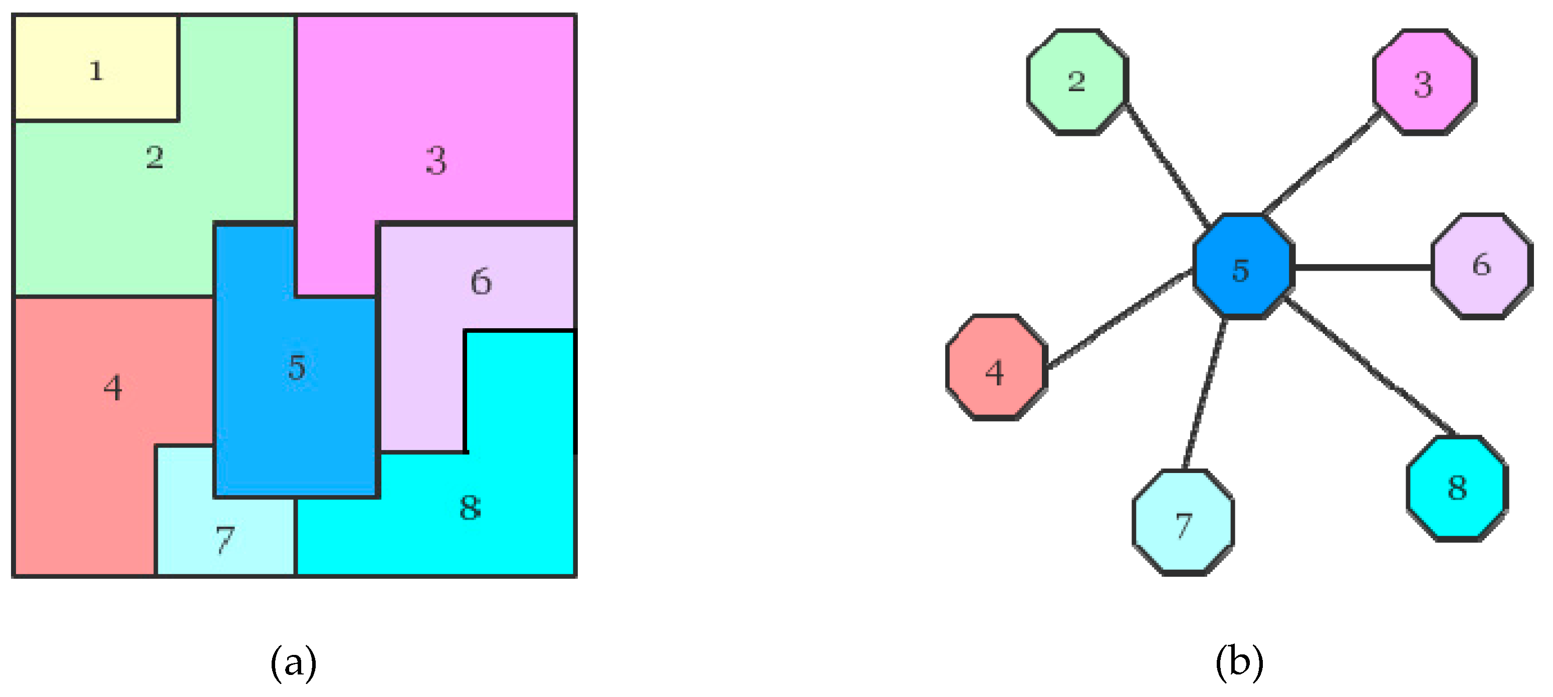
Then, the MAP criterion and the iterative conditional mode (ICM) [20,35,36] algorithm are used to adjust boundaries, which is called soft segmentation [20]. Note that in this step, at each iteration, the a posteriori probability of pixel i is only computed and compared within the neighborhood ${\eta }_a$ where the pixel belongs. The neighborhood system of a region is different from that of a pixel, as shown in Figure 3. At the end of each iteration, we will check the segmentation results and assign the area that is too small to the adjacent area. The purpose of this procedure is to reduce the computational cost and avoid isolated pixels. According to (17) and (21), the region label of pixel I is estimated as:

$$\begin{gathered} {\widehat{x}}_i=\arg \underset{x_i\in {\eta }_a}{\max }\left\{\frac{L^{qL}{\left|{\mathit{C}}_i\right|}^{L-q}\exp \{U_{edge}\left(x_i\right)-LTr\left({\mathbf{\Sigma }}_a^{-1}{\mathit{C}}_i\right)\}}{R\left(L,q\right){\left|{\mathbf{\Sigma }}_a\right|}^L{\displaystyle {\sum }_{x_i=1}^K\exp \left\{U_{edge}\left(x_i\right)\right\}}}\right\} \\ {\widehat{x}}_i=\arg \underset{x_i\in {\eta }_i}{\max }\left\{\begin{array}{l}\frac{2{\left|C_i\right|}^{L-q}\exp \left\{U_{edge}\left(x_i\right)\right\}}{R\left(L,q\right)\mathsf{\Gamma }\left(\sigma \right){\left|{\Sigma }_a\right|}^L{\displaystyle {\sum }_{x_i=1}^K\exp \left\{U_{edge}\left(x_i\right)\right\}}}{\left(L\sigma \right)}^{\frac{\sigma +Lq}{2}}\\ \cdot {\left(Tr\left({\Sigma }_a^{-1}{\mathit{C}}_i\right)\right)}^{\frac{\sigma -Lq}{2}}{K}_{\sigma -Lq}\left(2\sqrt{L\sigma Tr\left({\Sigma }_a^{-1}{C}_i\right)}\right)\end{array}\right\}, \end{gathered}$$

(22)

Note that Formula (22) is used to adjust the boundaries, not for classification. After the soft segmentation, each region is taken as a basic unit of the image. Then, the ML criterion is used to get the final classification result.

The procedure of the region-based classification is as follows:

• Divide the m × n image into $I=\lceil m/r\rceil \times \lceil n/r\rceil$ regions, which are not overlapping with each other. Let $X=\left\{x_a,a=1,\dots ,I\right\}$ denote the region labels.
• Calculate the mean covariance matrix ${\mathbf{\Sigma }}_a$ for each region.
• Use (22) to update the region boundaries.
• Check the segmentation result. If the region area is smaller than a threshold p, reassign it to the adjacent region. The parameter p decides the smallest area of a region.
• Check if the segmentation result is converged. If not, go back to Step 2. Otherwise, end the iteration, and the superpixels are obtained.
• Calculate the mean covariance matrix ${\mathbf{\Sigma }}_a$ of each region. Apply the ML classifier to get the final classification result.

4. Experiments and Discussions

4.1. Test Data

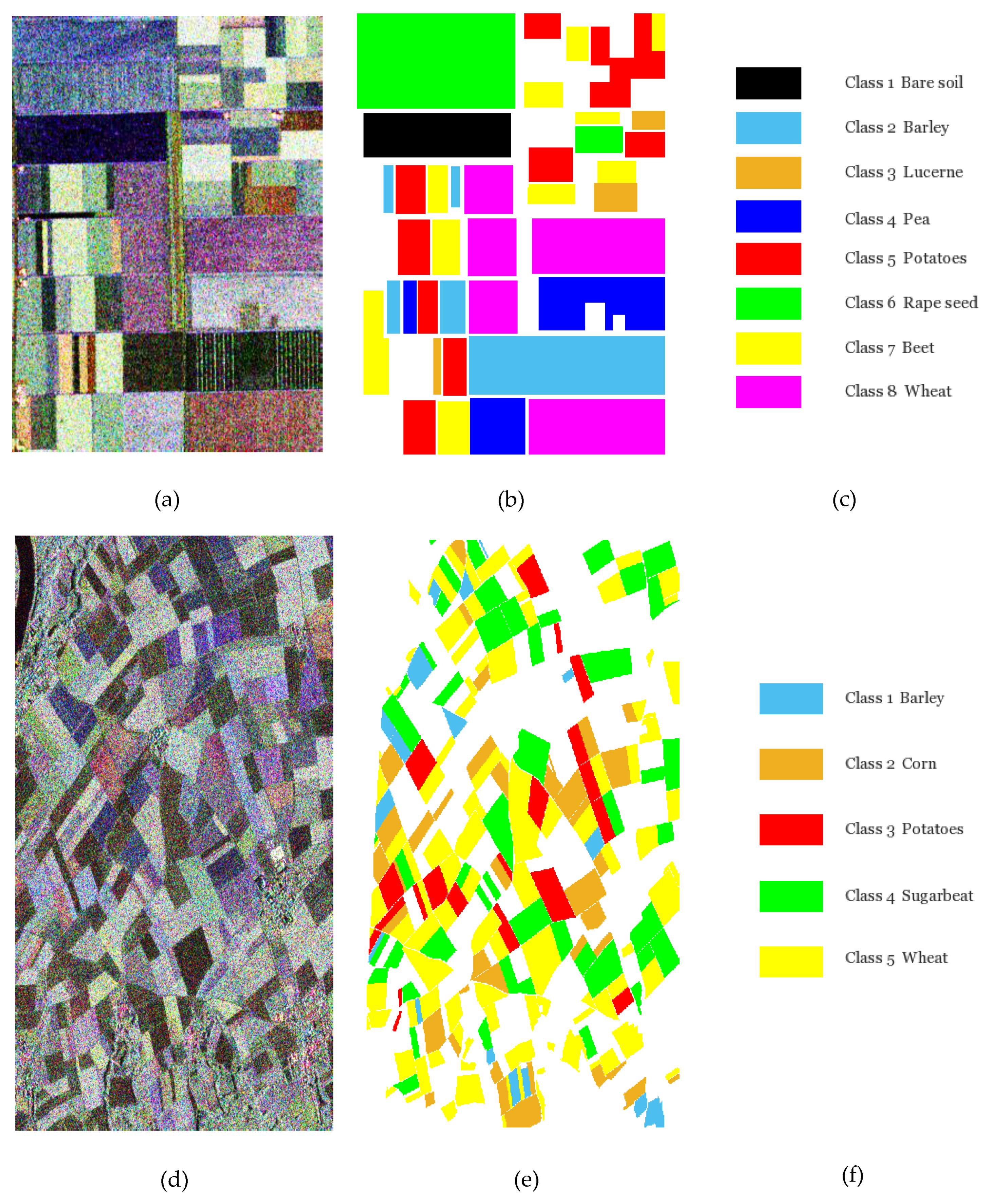
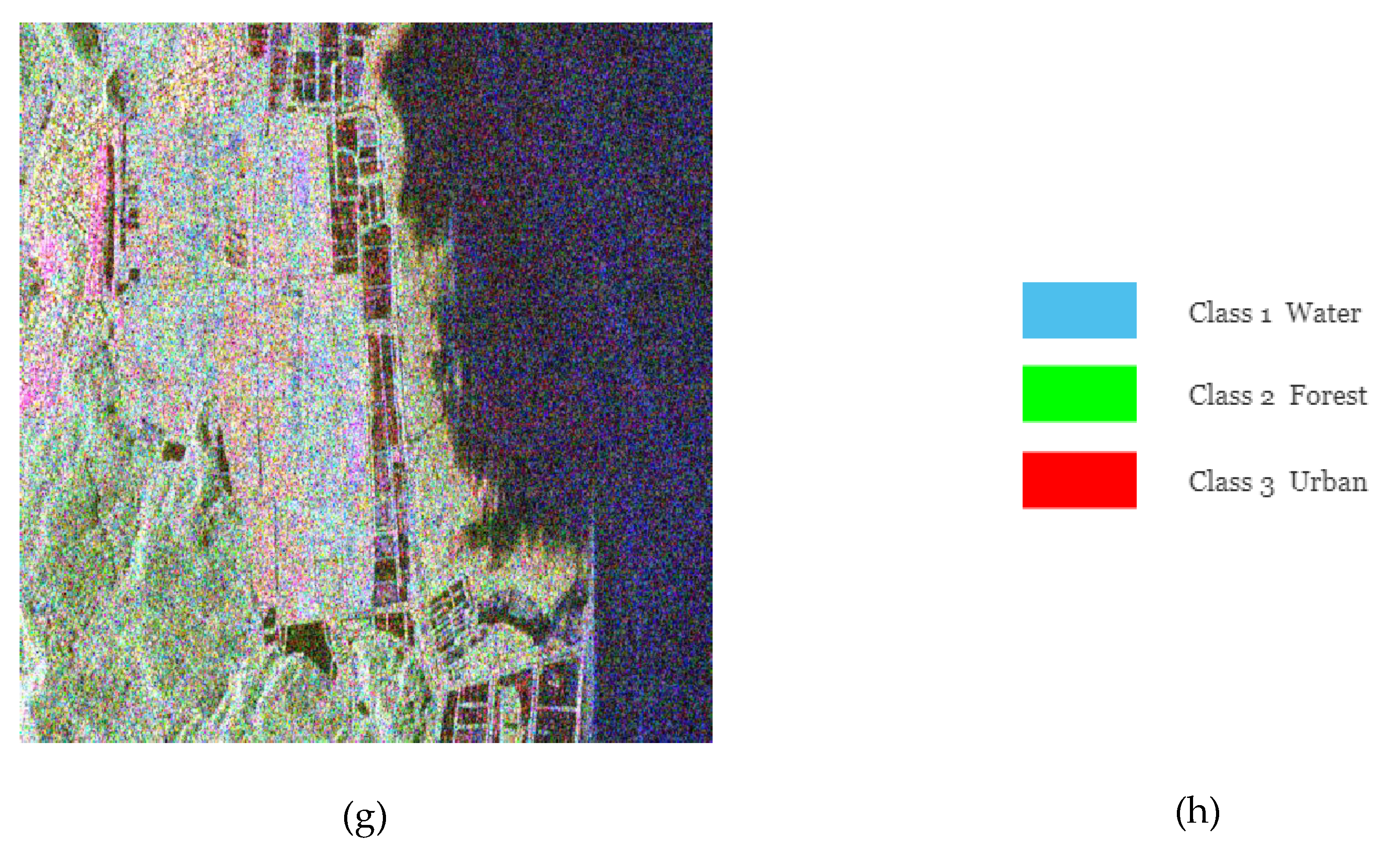
Polarimetric SAR data collected over two agricultural areas and a city were used for the experiments. The first were the L-band data from NASA/JPL AIRSAR collected over Flevoland Nederland in 1989. The Pauli color-coded figure and the ground truth map are shown in Figure 4a–c, which have 400 × 280 pixels. There was a total of 8 crop classes. The second dataset was from RADARSAT-2 acquired over Wallerfing, Germany. The beam pattern of this dataset had a fine beam of 8 m. The dataset was from an agriculture area, collected on May 28, 2014, with the incidence angle ranging from 40.2° to 41.6° on the descending pass. The size of the image was 920 × 500 pixels. This region had five classes according to the ground measure. The Pauli color-coded image and the ground truth map are shown in Figure 4d–f. The third dataset was from RADARSAT-2 acquired over Fujian Province, China. The dataset was from Fuzhou Langqi Island (center latitude: 26°03′ N, center longitude: 119°35′ W), collected on November 13, 2013. The resolution was around 8 m. The size of the image was 520 × 500 pixels. This region had 3 classes, including urban area, water, and forest. Because we did not have the ground truth map, we only provided the Pauli color-coded image in Figure 4g. All PolSAR images were filtered with the refined Lee filter with a 9*9 window before performing the classification. Our computer configuration was a Core i7 CPU clocked at 1.99 GHz, 1T hard drive, and 8G of memory.

The following methods were carried out in the experiments: the combination of the Wishart model and MRF (WMRF) for pixel-based classification, the combination of the K-Wishart model and MRF (KMRF) for pixel-based classification, the combination of the MWC model and MRF (MWMRF) for pixel-based classification, the combination of the MWC model and MRF without the edge penalty term (MWMRF/e) for pixel-based classification, the combination of the Wishart model and MRF (WMRF) for region-based classification, and the combination of the K-Wishart model and MRF (KMRF) for region-based classification.

4.2. Pixel-Based Classification

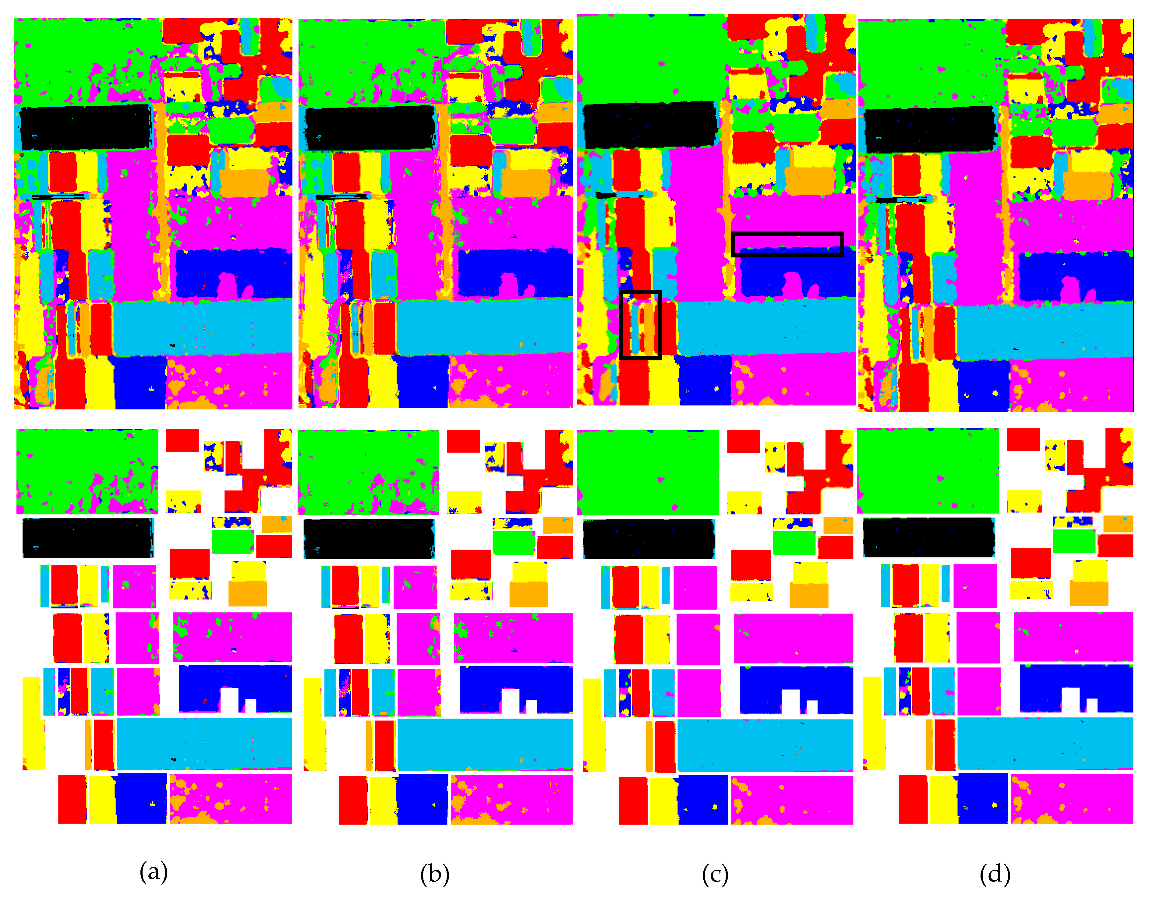
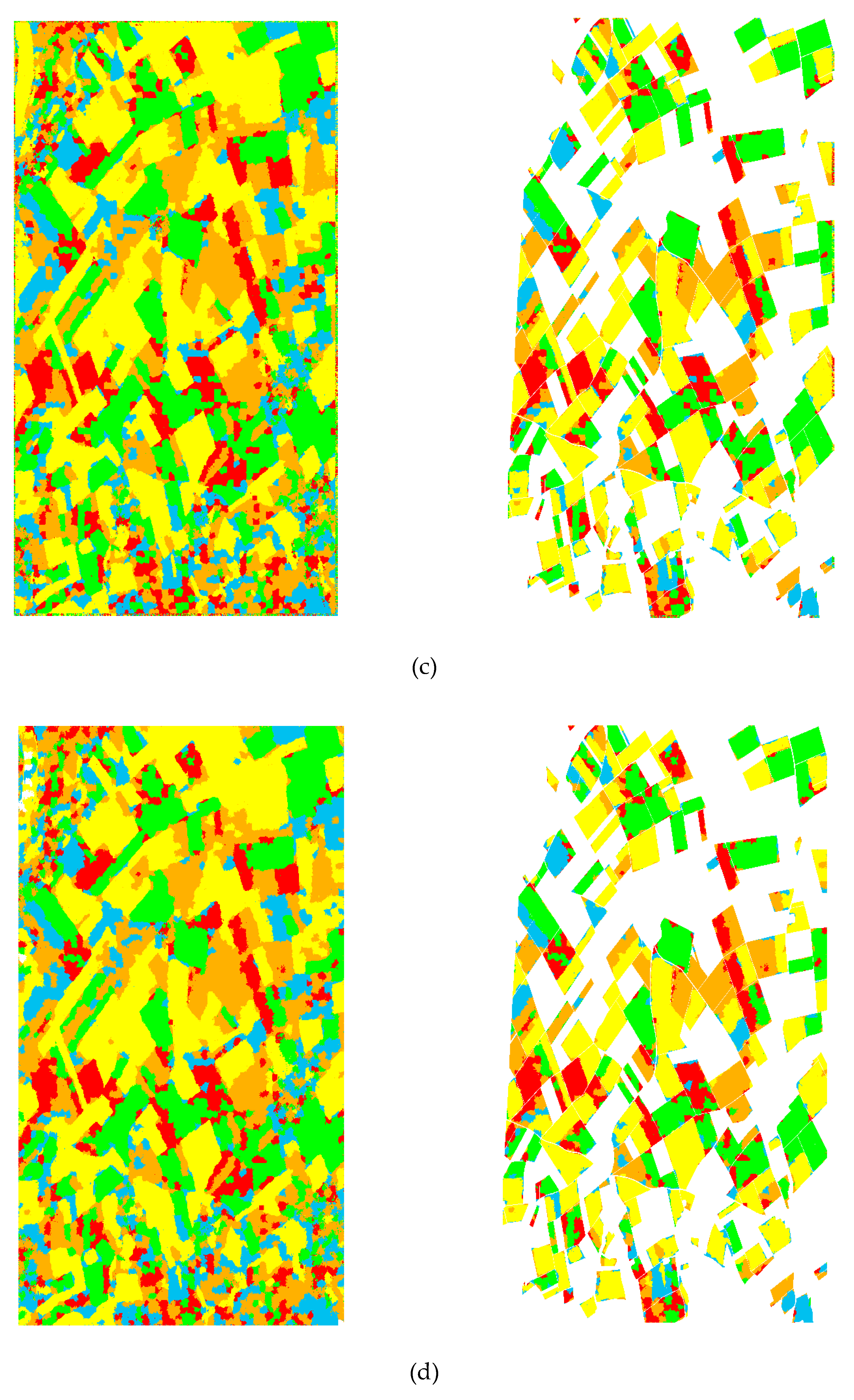
Classification results obtained by the pixel-based WMRF, KMRF, and MWMRF methods are shown in Figure 5a–c, Figure 6a–c, and Figure 7a–c. MWMRF/e denotes the MWMRF model without the edge penalty term, for which the experiment results are shown in Figure 5d, Figure 6d, and Figure 7d. The overall accuracy (OA) and the Kappa coefficients are given in

Table 1. Comparison of the pixel-based classification algorithms for the Flevoland data.

Method	Class 1 Bare Soil	Class 2 Barely	Class 3 Lucerne	Class 4 Pea	Class 5 Potatoes	Class 6 Rape Seed	Class 7 Beet	Class 8 Wheat	OA	Kappa
WMRF	97.56%	95.49%	93.83%	94.37%	92.51%%	87.88%	86.75%	90.30%	91.56%	0.9005
KMRF	97.58%	95.41%	94.10%	94.51%	92.39%	89.29%	88.35%	90.94%	92.12%	0.9071
MWMRF	97.59%	97.74%	95.64%	95.71%	95.49%	98.03%	93.25%	96.74%	96.44%	0.9580
MWMRF/e	97.37%	97.62%	95.00%	95.47%	94.97%	97.33%	92.65%	96.35%	96.02%	0.9530

and

Table 2. Comparison of the pixel-based classification algorithms for the Wallerfing dataset.

Method	Class1 Barley	Class 2 Corn	Class 3 Potatoes	Class 4 Sugar Beet	Class 5 Wheat	OA	Kappa
WMRF	88.31%	73.44%	58.81%	79.95%	92.38%	82.25%	0.7563
KMRF	88.24%	74.27%	61.59%	79.76%	92.19%	82.47%	0.7609
MWMRF	90.47%	79.15%	63.30%	83.79%	92.72%	84.40%	0.7854
MWMRF/e	86.13%	79.12%	48.98%	84.24%	95.13%	84.04%	0.7783

, respectively, for the Flevoland and Wallerfing datasets.

According to Figure 5 and Figure 6, we can see that the classification results by MWMRF were the best and had the highest OA and Kappa coefficients by quantitative comparison. Compared with other two models, MWMRF was better to fit the real PolSAR statistic. It was capable of capturing the spatial-contextual information, which could greatly reduce the effect of noise on the classification. As shown in Figure 5c,d and Figure 6c,d, there were more misclassified pixels around the edges in the MWMRF/e classification results as compared to those in the MWMRF classification results. In Figure 5c and Figure 6c, it is observed by the black squares that the classification map obtained by MWMRF was smoother, and the edge locations were more accurate. This proved that the edge penalty term had a good effect on the classification. Furthermore, Table 1 and Table 2 show that the classification results of MWMRF for both the Flevoland and Wallerfing datasets were better than the others for all classes. The OA and Kappa coefficients were 96.44% and 0.9580, respectively, for the Flevoland data, and 84.40% and 0.7854, respectively, for the Wallerfing data. As for the Fujian dataset, we only analyzed the results by visual inspection, since we did not have a real ground truth. According to Figure 7, the classification result by the MWMRF model was still the best, especially for urban area. The classification result of the MWMRF model had a better regional integrity and suffered less noise. Comparing Figure 7c with Figure 7d, we can see that the coastline and the edges between forest and urban were more accurate in Figure 7c. According to the above analysis, we can see that the MWMRF model was also effective for a heterogeneous region with a complex shape. The computational cost was 3 min for WMRF, 17.5 min for KMRF, and 20.8 min for MWMRF. This shows that MWMRF was a robust and efficient pixel-based classification algorithm for PolSAR images.

4.3. Region-Based Classification

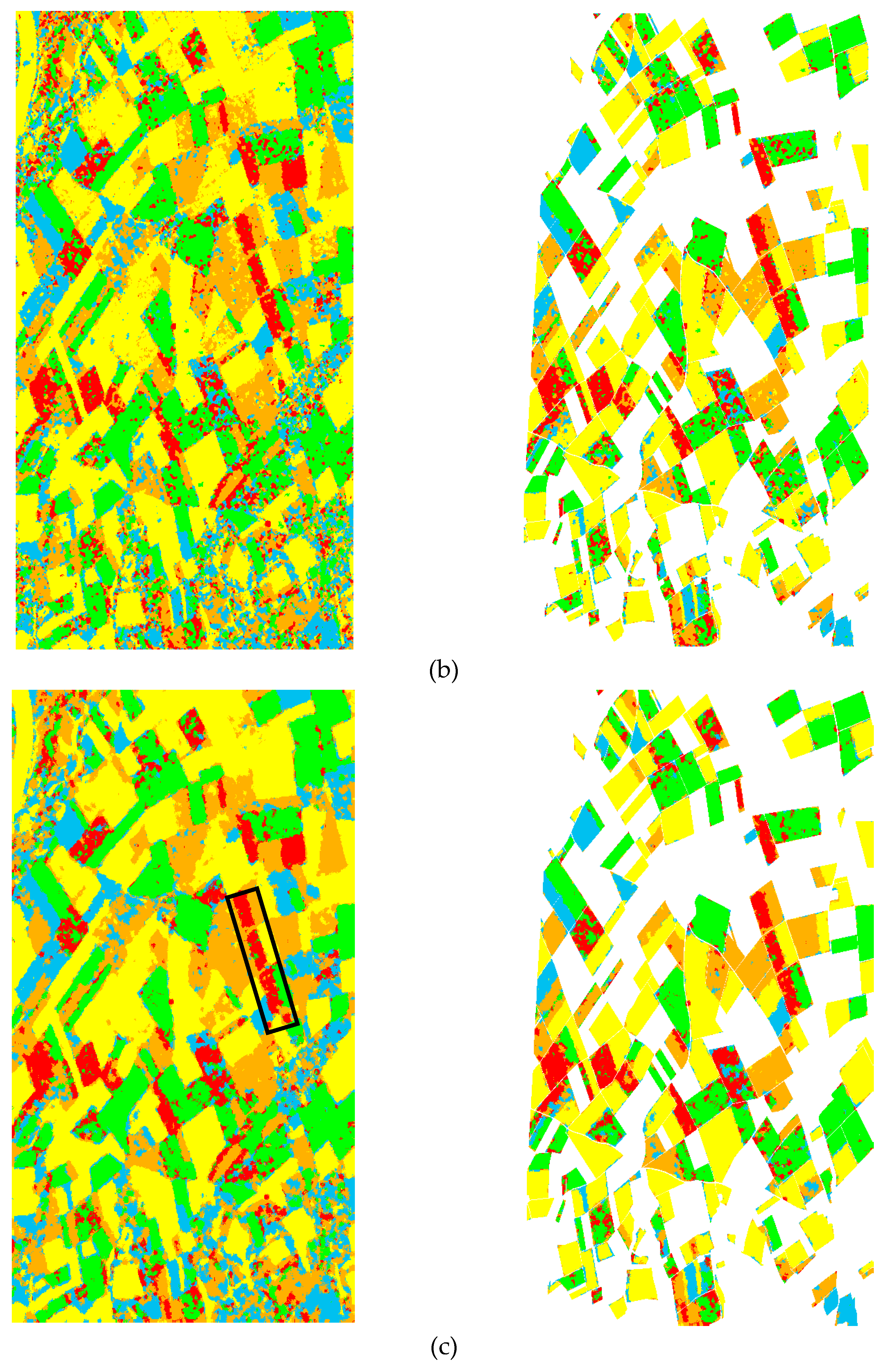
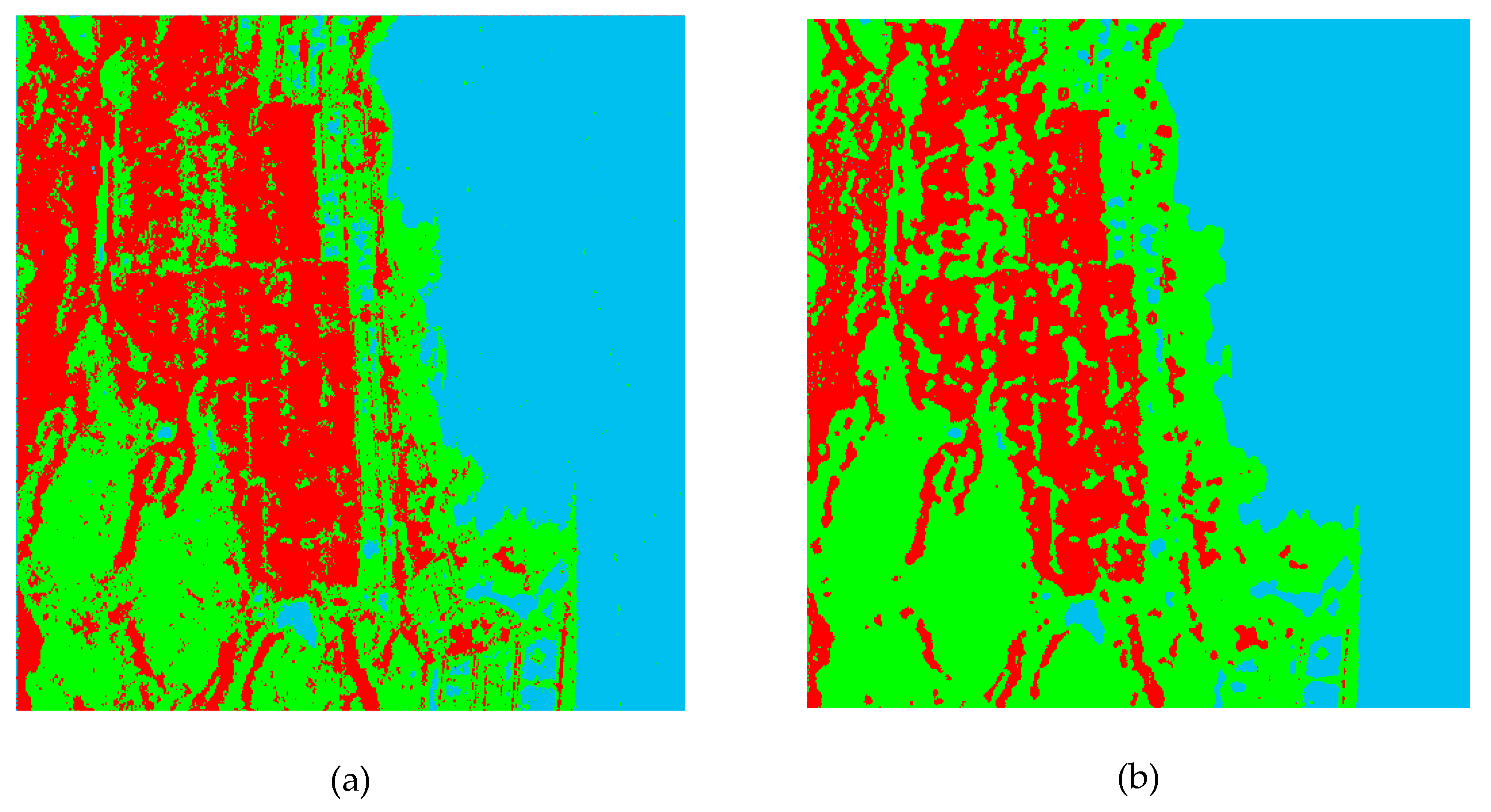
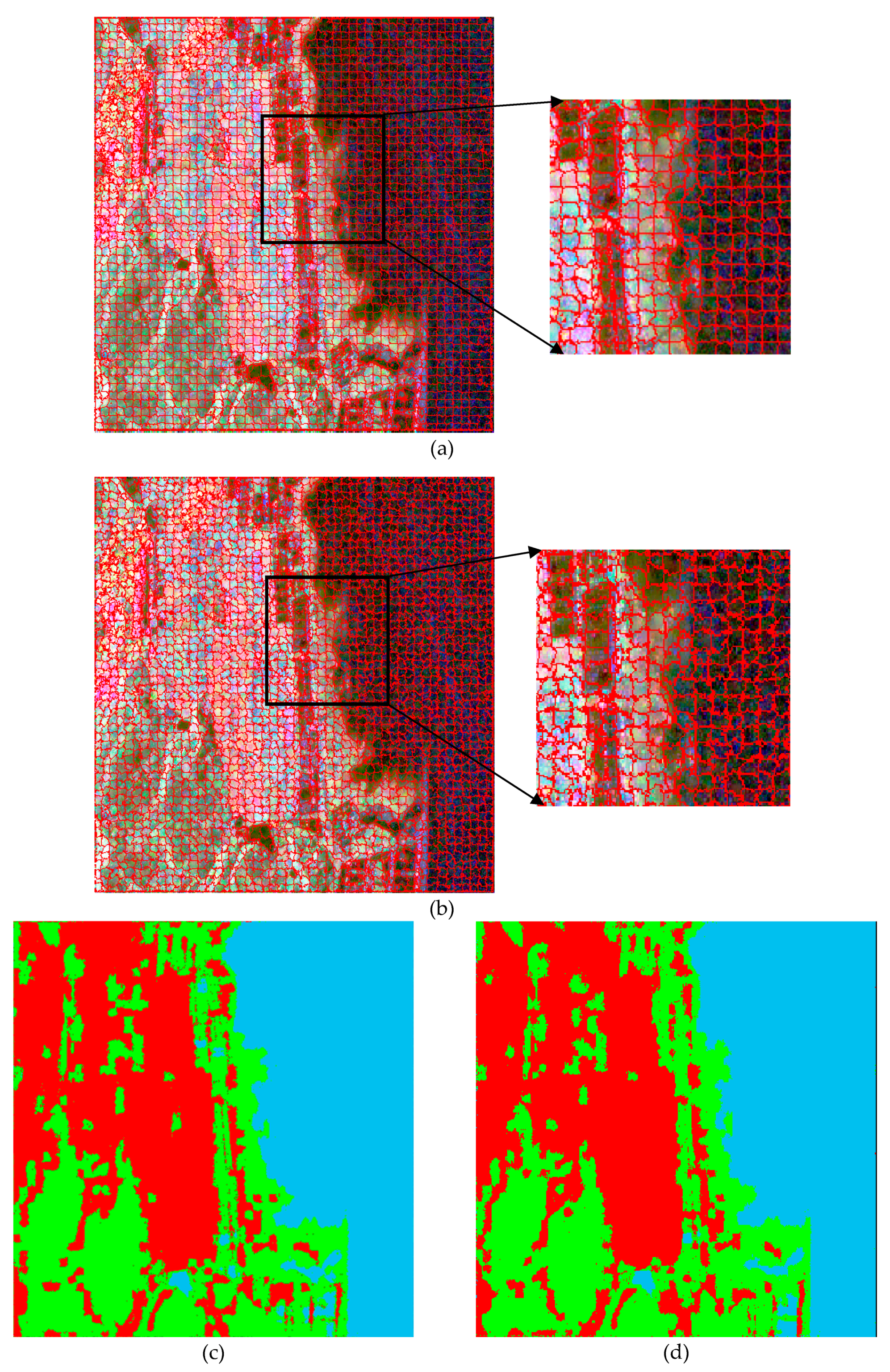
The classification results obtained by region-based methods are shown in Figure 7 and Figure 8. We set r = 10 and p = 25 in this study. The image was firstly divided into many 10 × 10 rectangles, and then, MRF models were used to adjust the boundaries. We assumed the area of a region to be no less than 25 pixels. The segmentation results are in Figure 8a,b, Figure 9a,b, and Figure 10a,b. The final classification maps were obtained based on the segmentation results using the Wishart-based ML algorithm, which are shown in Figure 8c,d, Figure 9c,d, and Figure 10c,d.

Table 3. Comparison of the region-based classification algorithms for the Flevoland data.

Method	Class 1 Bare Soil	Class 2 Barely	Class 3 Lucerne	Class 4 Pea	Class 5 Potatoes	Class 6 Rape Seed	Class 7 Beet	Class 8 Wheat	OA	Kappa
WMRF	99.64%	95.35%	91.87%	90.77%	99.95%	93.00%	93.00%	88.59%	93.46%	0.9231
KMRF	97.01%	87.37%	84.69%	89.58%	89.41%	98.24%	87.63%	87.93%	90.45%	0.8879

and

Table 4. Comparison of the region-based classification algorithms for the Wallerfing data.

Method	Class1 Barley	Class 2 Corn	Class 3 Potatoes	Class 4 Sugar Beet	Class 5 Wheat	OA	Kappa
WMRF	86.41%	75.40%	70.91%	84.20%	89.29%	83.62%	0.7763
KMRF	86.03%	75.07%	70.10%	82.10%	89.57%	83.20%	0.7706

give the OA and the Kappa coefficients for the Flevoland and Wallerfing data classification results.

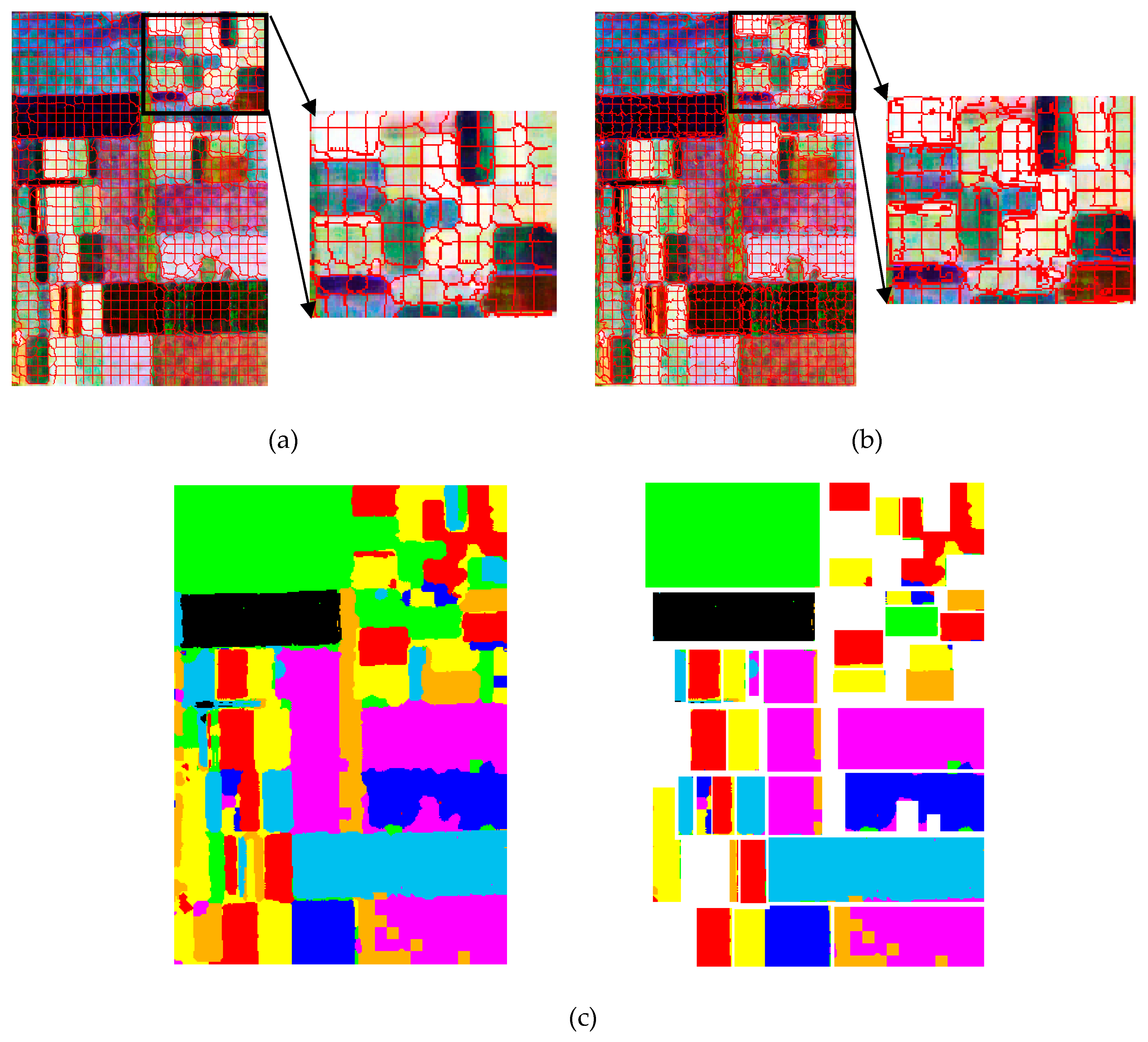
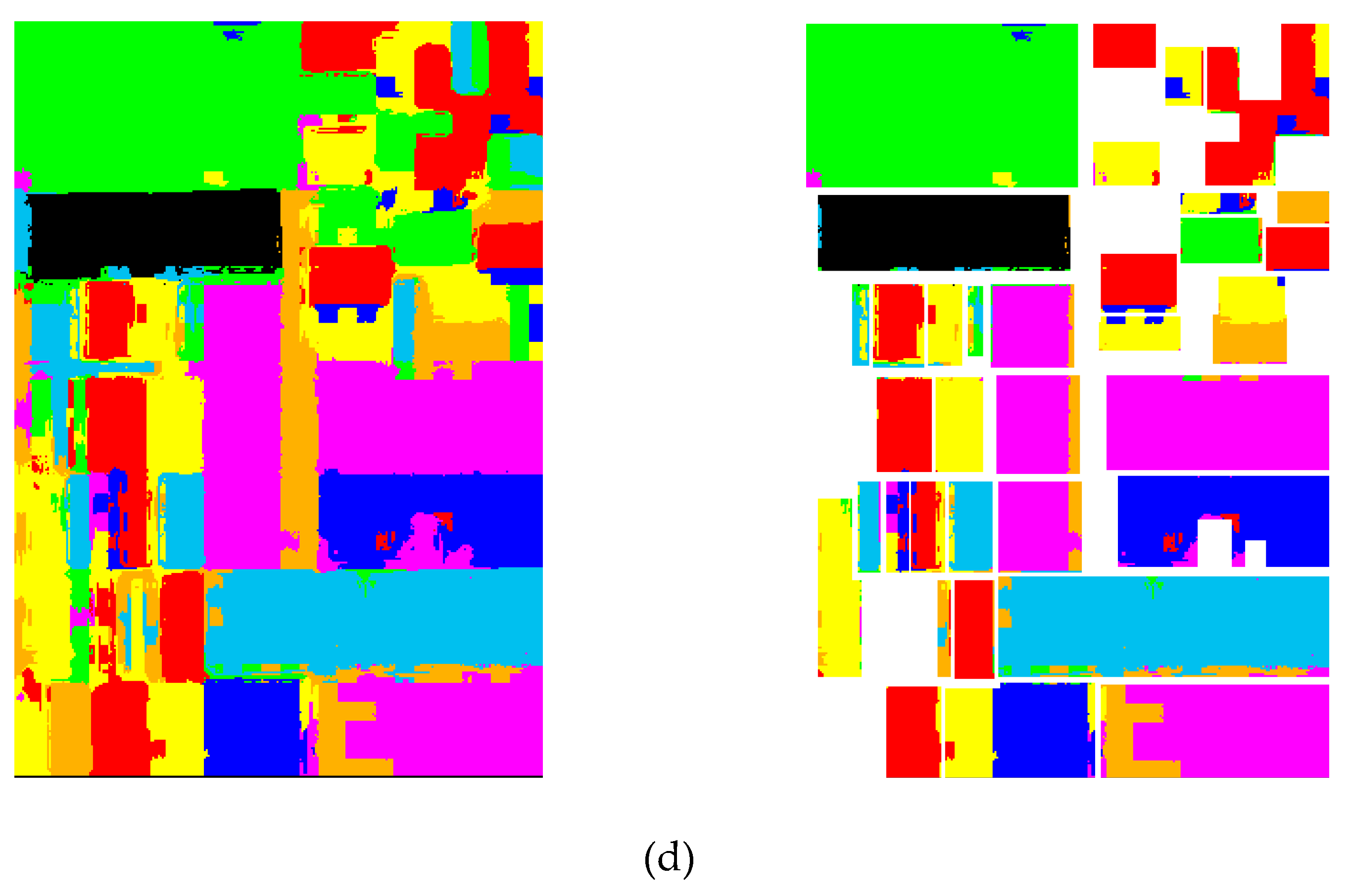
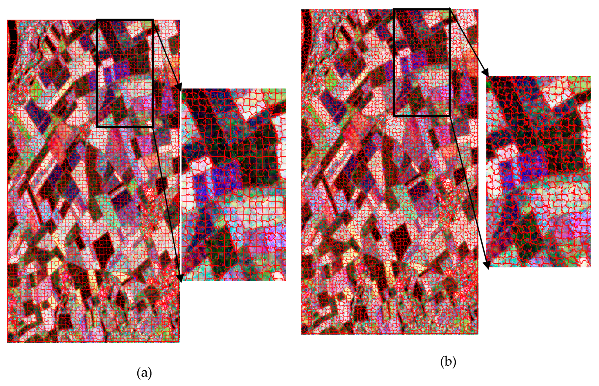
As shown in Figure 8c,d and Figure 9c,d, the edges of the KMRF classification map were more accurate, especially for the Flevoland dataset. As for the Fujian dataset, regions were irregularly shaped, and the edges between different areas were not very clear. By visual inspection, the classification results of WMRF and KMRF did not have much difference. However, by a close comparison, it can be seen from the segmentation results in Figure 8a,b, Figure 9a,b, and Figure 10a,b that segmentation based on the WMRF model was more homogenous and the edges of the region more complete. In comparison, the segmentation results of the KMRF model were not smooth enough and were sensitive to image textures. Since the classification result of the region-based algorithm largely depended on the segmentation result, the classification maps of the WMRF model were better. The evaluations in Table 3 and Table 4 also prove this. The OA and Kappa coefficients of WMRF were 93.46% and 0.9231, respectively, for the Flevoland data, and 83.62% and 0.7763, respectively, for the Wallerfing data, respectively. Although the classification accuracy and Kappa coefficients of both models were close, the classification accuracy of the WMRF model was robustly higher. Moreover, the K-Wishart distribution was more complex than the Wishart distribution. The computational cost was 18 min for WMRF and 5.3 h for KMRF. The segmentation algorithm based on KMRF consumed more time.

4.4. Discussions

We compared the pixel-based and region-based classification algorithms based on the WMRF and KMRF models. From visual inspection, it showed that the region-based algorithm was better at classifying the Flevoland data. The misclassifications caused by image textures and speckle noise were noticeably reduced. We also performed the McNemar test on the classification results of the region-based algorithm and pixel-based algorithm. The test statistics was 8.85e-81 for pixel-based and region-based WMRF and 7.55e-72 for pixel-based and region-based KMRF. The critical level was set to 0.05. It was found that for both WMRF and KMRF methods, the region-based and pixel-based classification results had different proportions of errors. As for the Wallerfing data, the results were reversed. From Table 2 and Table 4, it is shown that the OA and Kappa coefficients of the pixel-based method were higher. That was because the fields in the Wallerfing dataset were small and irregularly shaped, and the edges were weak, which made it difficult for image segmentation. The region-based classification method took a region as the basic image unit. Therefore, inaccurate segmentation could result in multiple classes within a region, which would cause misclassification. The Fujian dataset had heterogeneous regions with irregular shapes. The weak edges between regions also increased the difficulty in image segmentation. However, the area of different regions was relatively large, which made it easier for image segmentation than that of the Wallerfing data. The classification maps of the region-based algorithm also showed a higher region integrity than that of pixel-based algorithms. For the time consumption, the region-based algorithms consumed more time than the pixel-based algorithms. The equipment configuration we used in the experiment was a laptop, which took more time. In actual applications, using better configuration equipment may solve the time consumption problem. Therefore, the region-based algorithm was more suitable for the Fujian dataset. In conclusion, the pixel-based method was more suitable for the Wallerfing dataset, and the region-based method was more suitable for the Flevoland and Fujian datasets.

5. Conclusions

This paper studied the MRF-based algorithms for PolSAR image classification. Three statistical distributions, including the Wishart, K-Wishart, and mixture Wishart models, were combined with MRF to implement the pixel-based and region-based classifications. A new mixture strategy was proposed for the MRF model, with its performance evaluated based on real PolSAR images. It was found that using a Wishart mixture distribution to model a class performed better than that to model a whole image. The adaptive neighborhood and an edge penalty term were also employed in the MRF energy functional for the better location of edges. The Wishart and K-Wishart distributions served as the likelihood term in the MRF framework, while for the mixture model, MRF was embedded into each component of the statistics to construct the MWMRF. Landcover classification is always a challenging task. In experiments, real PolSAR images acquired over an island and agricultural fields with irregular shapes were used for demonstration. It was observed from the results that the MWMRF model showed the best classification results in pixel-based methods. For region-based methods, the OA and Kappa coefficients of the WMRF model were higher than those of KMRF. Moreover, WMRF had time efficiency.

The pixel-based methods were better in preserving image details such as boundary locations. However, there existed noise (isolated class labels or small groups of misclassifications) in the classification maps. The region-based methods took region blocks as the classification unit, so the results obtained by these kinds of methods have less noise in the classified maps. However, the final classification results were largely dependent on the segmentation results. Experiments showed that the pixel-based MWMRF model was suitable for small and irregularly shaped field classification, and the region-based WMRF model could be used for classification of evenly distributed farmlands and urban areas.

References

- Moreira, A.; Prats-Iraola, P.; Younis, M. A tutorial on synthetic aperture radar. IEEE Geosci. Remote Sens. Mag. 2013, 1, 6–43. [Google Scholar] [CrossRef] [Green Version]
- Cloude, S.R. Polarisation: Applications in Remote Sensing, 1st ed.; Oxford University Press: New York, NY, USA, 2010. [Google Scholar]
- Lee, J.S.; Grunes, M.R.; Pottier, E. Quantitative comparison of classification capability: Fully polarimetric versus dual and single-polarization SAR. IEEE Trans. Geosci. Remote Sens. 2001, 39, 2343–2351. [Google Scholar]
- Lee, J.S.; Grunes, M.R.; Ainsworth, T.L. Quantitative comparison of classification capability:fully-polarimetric versus partially polarimetric SAR. In Proceedings of the IEEE International Geoscience & Remote Sensing Symposium, Toronto, ON, Canada, 24–28 June 2002. [Google Scholar]
- Kong, J.A.; Swartz, A.A.; Yueh, H.A. Identification of terrain cover using the optimum polarimetric classifier. J. Electromagn. Waves Appl. 1988, 2, 171–194. [Google Scholar]
- Yin, J.; Moon, W.M.; Yang, J. Novel model-based method for identification of scattering mechanisms in polarimetric SAR data. IEEE Trans. Geosci. Remote Sens. 2016, 54, 520–532. [Google Scholar] [CrossRef]
- Lee, J.S.; Hoppel, K.; Mango, S.A. Intensity and phase statistics of multi-look polarimetric SAR imagery. IEEE Trans. Geosci. Remote Sens. 1994, 32, 1017–1028. [Google Scholar]
- Lee, J.S.; Mitchell, R.G.; Kwok, R. Classification of multi-look polarimetric SAR imagery based on complex Wishart distribution. Int. J. Remote Sens. 1994, 15, 2299–2311. [Google Scholar] [CrossRef]
- Jao, J. Amplitude distribution of composite terrain radar clutter and the κ-Distribution. IEEE Trans. Antennas Propag. 1984, 32, 1049–1062. [Google Scholar]
- Lee, J.S.; Schuler, D.L.; Lang, R.H.; Ranson., K.J. K-Distribution for Multi-Look Processed Polarimetric SAR Imagery. In Proceedings of the IEEE International Geoscience and Remote Sensing Symposium, Pasadena, PA, USA, 8–12 August 1994; pp. 2179–2181. [Google Scholar]
- Freitas, C.C.; Frery, A.C.; Correia, A.H. The polarimetric G distribution for SAR data analysis. Environmetrics 2005, 16, 13–31. [Google Scholar] [CrossRef]
- McLachlan, G.J.; Peel, D. Finite Mixture Models; Wiley: New York, NY, USA, 2000. [Google Scholar]
- Doulgeris, A.P.; Anfinsen, S.N.; Eltoft, T. Classification with a non-Gaussian model for PolSAR data. IEEE Trans. Geosci. Remote Sens. 2008, 46, 2999–3009. [Google Scholar] [CrossRef] [Green Version]
- Gao, W.; Yang, J.; Ma, W. Land Cover Classification for Polarimetric SAR Images Based on Mixture Models. Remote Sens. 2014, 6, 3770–3790. [Google Scholar] [CrossRef] [Green Version]
- Doulgeris, A.P.; Anfinsen, S.N.; Eltoft, T. Automated non-Gaussian clustering of polarimetric synthetic aperture radar images. IEEE Trans. Geosci. Remote Sens. 2011, 49, 3665–3676. [Google Scholar] [CrossRef]
- Li, S.Z. Markov Random Field Modeling in Image Analysis; Springer: London, UK, 2009. [Google Scholar]
- Yamazaki, T.; Gingras, D. Image Classification Using Spectral and Spatial Information Based on MRF Models. IEEE Trans. Image Process. A Publ. IEEE Signal Process. Soc. 1995, 4, 1333–1339. [Google Scholar] [CrossRef] [PubMed] [Green Version]
- Deng, H.; Clausi, D.A. Gaussian MRF rotation-invariant features for image classification. IEEE Trans. Pattern Anal. Mach. Intell. 2004, 26, 951–955. [Google Scholar] [CrossRef] [PubMed]
- Dong, Y.; Milne, A.K.; Forster, B.C. Segmentation and classification of vegetated areas using polarimetric SAR image data. IEEE Trans. Geosci. Remote Sens. 2001, 39, 321–329. [Google Scholar] [CrossRef]
- Wu, Y.; Ji, K.; Yu, W. Region-Based Classification of Polarimetric SAR Images Using Wishart MRF. IEEE Geosci. Remote Sens. Lett. 2008, 5, 668–672. [Google Scholar] [CrossRef]
- Liu, G.; Li, M.; Wu, Y. PolSAR image classification based on Wishart TMF with specific auxiliary field. IEEE Geosci. Remote Sens. Lett. 2014, 11, 1230–1234. [Google Scholar]
- Shi, J.; Li, L.; Liu, F. Unsupervised polarimetric synthetic aperture radar image classification based on sketch map and adaptive Markov random field. J. Appl. Remote Sens. 2016, 10, 025008. [Google Scholar] [CrossRef]
- Masjedi, A.; Zoej, M.J.V.; Maghsoudi, Y. Classification of polarimetric SAR images based on modeling contextual information and using texture features. IEEE Trans. Geosci. Remote Sens. 2015, 54, 932–943. [Google Scholar] [CrossRef]
- Li, W.; Prasad, S.; Fowler, J.E. Hyperspectral image classification using Gaussian mixture models and Markov random fields. IEEE Geosci. Remote Sens. Lett. 2014, 11, 153–157. [Google Scholar] [CrossRef] [Green Version]
- Song, W.; Li, M.; Zhang, P. Mixture WGΓ-MRF Model for PolSAR Image Classification. IEEE Trans. Geosci. Remote Sens. 2017, 56, 905–920. [Google Scholar] [CrossRef]
- Lee, J.S.; Pottier, E. Polarimetric Radar Imaging: From Basic to Application; CRC Press: New York, NY, USA, 2011. [Google Scholar]
- Yang, W.; Yang, X.; Yan, T. Region-Based Change Detection for Polarimetric SAR Images Using Wishart Mixture Models. IEEE Trans. Geosci. Remote Sens. 2016, 54, 6746–6756. [Google Scholar] [CrossRef]
- Sherman, S. Markov random fields and gibbs random fields. Isr. J. Math. 1973, 14, 92–103. [Google Scholar] [CrossRef]
- Rignot, E.; Chellappa, R. Segmentation of polarimetric synthetic aperture radar data. IEEE Trans. Image Process. 1992, 1, 281–300. [Google Scholar] [CrossRef] [PubMed]
- Smits, P.C.; Dellepiane, S.G. Synthetic aperture radar image segmentation by a detail preserving Markov random field approach. IEEE Trans. Geosci. Remote Sens. 1997, 35, 844–857. [Google Scholar] [CrossRef]
- Niu, X.; Ban, Y. A novel contextual classification algorithm for multitemporal polarimetric SAR data. IEEE Geosci. Remote Sens. Lett. 2014, 11, 681–685. [Google Scholar]
- Fjortoft, R.; Lopes, A.; Marthon, P.; Cubero-Castan, E. An optimal multiedge detector for SAR image segmentation. IEEE Trans. Geosci. Remote Sens. 1998, 36, 793–802. [Google Scholar] [CrossRef] [Green Version]
- Schou, J.; Skriver, H.; Nielsen, A.A. CFAR edge detector for polarimetric SAR images. IEEE Trans. Geosci. Remote Sens. 2003, 41, 20–32. [Google Scholar] [CrossRef] [Green Version]
- Geman, S.; Geman, D. Gibbs Distributions, and the Bayesian Restoration of Images. Read. Comput. Vis. 1984, 20, 25–62. [Google Scholar]
- Kottke, D.P.; Fiore, P.D.; Brown, K.L.; Fwu, J.K. A design for HMM-based SAR ATR. In Proceedings of the SPIE—Conference Algorithms Synthetic Aperture Radar Imagery V, Orlando, FL, USA, 13 April 1998; Volume 3370, pp. 541–551. [Google Scholar]
- Besag, J. On the statistical analysis of dirty pictures. J. R. Stat. Soc. 1986, 48, 259–302. [Google Scholar] [CrossRef] [Green Version]
Figure 1.
Classification results of the two mixture algorithms. (a) Pauli color-coded image. (b) Mixture Wishart for a whole image (MWW). (c) mixture Wishart for a class (MWC). (d) Class legend.
Figure 2.
Five candidates of the adaptive neighborhood.
Figure 3.
Schematic representation for a region neighborhood. (a) Segmentation result. (b) The neighborhood system for Region 5.
Figure 4.
Polarimetric datasets used for the experiments. (a) Pauli color-coded image of the Flevoland data. (b) Ground truth map of Flevoland. (c) Class legend. (d) Pauli color-coded image of the Wallerfing data. (e) Ground truth map of Wallerfing. (f) Class legend. (g) Pauli color-coded image of the Fujian data.
Figure 5.
Pixel-based classification results of the Flevoland data. The first row shows the classification results, and the second row shows the corresponding classification results where the ground-truth map exists. (a) Wishart-MRF (WMRF). (b) K-Wishart-MRF (KMRF). (c) Wishart-MRF (MWMRF). (d) MWMRF model without the edge penalty term (MWMRF/e).
Figure 6.
Pixel-based classification results for the Wallerfing data. The left column shows the classification results, and the right column shows the corresponding classification results where the ground-truth map exists. (a) WMRF. (b) KMRF. (c) MWMRF. (d) MWMRF/e.
Figure 7.
Pixel-based classification results for the Fujian data. (a) WMRF. (b) KMRF. (c) MWMRF. (d) MWMRF/e.
Figure 8.
Region-based segmentation and classification results of the Flevoland area. (a,b) Segmentation results of the whole image. (a) WMRF. (b) KMRF. (c) Classification result with WMRF. (d) Classification result with KMRF.
Figure 9.
Region-based segmentation and classification results of the Wallerfing area. (a,b) Segmentation results of the whole image. (a) WMRF. (b) KMRF (c) Classification result with WMRF. (d) Classification result with KMRF.
Figure 10.
Region-based segmentation and classification results of the Fujian dataset. (a,b) Segmentation results of the whole image. (a) WMRF. (b) KMRF (c) Classification result with WMRF. (d) Classification result with KMRF.