Analyzing the Angle Effect of Leaf Reflectance Measured by Indoor Hyperspectral Light Detection and Ranging (LiDAR)

Abstract

Hyperspectral light detection and ranging (LiDAR) (HSL) combines the characteristics of hyperspectral imaging and LiDAR techniques into a single instrument without any data registration. It provides more information than hyperspectral imaging or LiDAR alone in the extraction of vegetation physiological and biochemical parameters. However, the laser pulse intensity is affected by the incident angle, and its effect on HSL has not yet been fully explored. It is important for employing HSL to investigate vegetation properties. The aim of this paper is to study the incident angle effect of leaf reflectance with HSL and build a model about this impact. In this paper, we studied the angle effect of leaf reflectance from indoor HSL measurements of individual leaves from four typical tree species in Beijing. We observed that (a) the increasing of incident angle decreases the leaf reflectance; (b) the leaf spectrum observed by HSL from 650 to 1000 nm with 10 nm spectral resolution (36 channels) are consistent with those that measured by Analytica Spectra Devices (ASD) spectrometer (R² = 0.9472 ~ 0.9897); (c) the specular reflection is significant in the red bands, and clear non-Lambertian characteristics are observed. In the near-infrared, there is little specular reflection, but it follows the Lambert-scattering law. We divided the whole band (650–1000 nm) into six bands and established an empirical model to correct the influence of angle effect on the reflectance of the leaf for HSL applications. In the future, the calibration of HSL measurements applied for other targets will be studied by rigorous experiments and modelling.

1. Introduction

Hyperspectral imager is a passive and non-invasive remote sensing sensor with nanometer (nm) resolution, which obtains abundant and detailed spectral information of a target [1]. Recently, hyperspectral remote sensing has become an important method of earth observation in surface vegetation, and it has been proved in a number of successful studies, such as mineral identification, vegetation detection, and target classification [2,3,4], etc. However, passive remote sensing cannot avoid the effects of light source conditions and shadows, which has limited its broad successful applications. Moreover, it cannot provide the structural information of the target. In contrast to passive sensors, active hyperspectral sensors emit the laser pulse to the target and detect the echoes reflected from the target [1].

Light detection and ranging (LiDAR) is an efficient active remote sensing technology, which can accurately measure the distance to the target object and then generate three-dimensional point cloud. It has advanced the development in 3D information acquisition and topographic and geomorphic information acquisition [5,6]. LiDAR sensors are insensitive to the environmental illumination change. However, due to the limitation of laser light sources, traditional LiDAR sensors usually work in a single wavelength; therefore, they cannot provide abundant spectral information [7,8,9]. Compared with the passive hyperspectral sensor that can include hundreds of spectral channels, the spectral information of single-wavelength LiDAR is limited obviously. Therefore, compared with traditional single-wavelength LiDAR sensors, the point cloud information with rich spectral information will undoubtedly classify targets more effectively [4,10], such as cover classification [11], rangeland vegetation classification [12], etc. In previous studies in remote sensing, lots of results prove that the performance of traditional LiDAR and hyperspectral data fusion is better than any single sensor, such as land classification, and vegetation classification [11,12]. However, simple combination of hyperspectral and LiDAR data from two individual instruments cannot tackle the registration problem [8,13]. Therefore, the fusion of hyperspectral and LiDAR sensors has become the research hotspot in the community [1].

Hyperspectral LiDAR system combines the active hyperspectral imaging technique and LiDAR distance measuring technique into a single instrument framework with fine spectral resolution. Through commercial supercontinuum (SC) laser sources, hyperspectral LiDAR (HSL) emits the laser pulses and receives its echo, which includes high spectral information of the target and the LiDAR echo information, in order to obtain the geometrical characteristics of the target, such as the spatial information and spectral information [14]. This method is a perfect fusion of accurate three-dimensional information from LiDAR and hyperspectral information [1]. Given the advantage of not relying on sunlight and not being affected by the observed geometric information, hyperspectral LiDAR can obtain the three-dimensional structure and spectral information of understory vegetation [8].

A two-channel HSL was developed and tested in Finland in 2010, in which optical filters were utilized as a spectroscopic device [8]. HSL hardware prototype in full band was designed at the Finnish Geodetic Institute, which was used for vegetation remote sensing in 2012 [13]. Recently, various applications of HSL have been reported, such as coal/rock classification [15], vegetation detection [14], vegetation index extraction [16], architecture preservation [17], and ore classification [18].

Recently, terrestrial LiDAR with multiple-wavelength information was proved to be an effective way to combine the structural and spectral information. However, the effect of measurement geometry on LiDAR echo need to be studied further, such as the incidence angle, which plays an important role in the interaction of laser and target. Incidence angle is defined as the angle between the laser incidence direction and the normal direction of the target surface. Many studies have been made on the angle effect of monochromatic laser scanners, which aimed for the calibration and improvement of the laser scan results, such as the role of surface irregularities on the intensity data and the influence of the local scan geometry on the signal to noise ratio [19,20,21,22]. However, there is few researches using multispectral and hyperspectral LiDAR. New results about hyperspectral LiDAR measurements with 8-channel emerges recently [10], but the information of more different bands is needed in the research of the incidence angle effect. Furthermore, the effect for different leaves is also not yet completely understood. In former researches, the leaf is approximately considered to depend on the Lambert’s law. Therefore, researchers believe that the measured reflectance is only affected by the species of target leaf rather than the incidence angle [23].

However, there is no study on exploring the angle effect on the continuous full-band HSL so far. Thus, there is a growing need for systematic experiments on the effects of leaf geometry and structure on laser return intensity in full-band HSL. Full-band information is used in our research, and more available spectral information of different leaf species can be used to study the change of backscattering in different bands, and the angle effect of HSL can be corrected in the whole band using the model.

The main goal of this paper is to explore the effect of measurement geometry on echo intensity retrieved by a hyperspectral LiDAR instrument. We study the effect of incidence angle on laser backscatter from different leaves at different wavelengths and establish a reflectance correction model for hyperspectral LiDAR with different leaf inclinations at different wavelengths.

2. Material and Methods

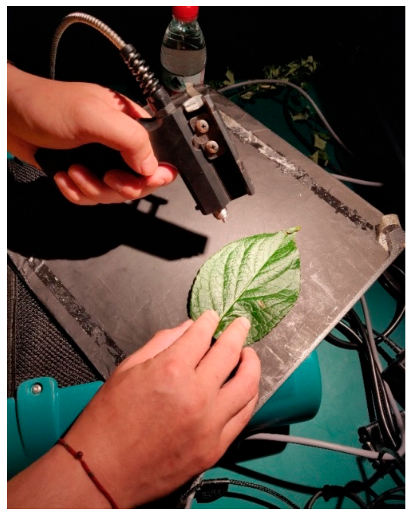
2.1. Material Preparation and Measurement

2.1.1. Leaf Samples

In this experiment, we selected five leaves of common four tree species in Beijing (

Table 1. Leaf samples and corresponding pictures (Red dots are the laser scanning points).

Leaf Samples	Fraxinus pennsylvanica	Eucommia ulmoides	Amygdalus triloba	Fraxinus pennsylvanica (yellow leaf)	Magnolia denudata
Photos

) as observation targets. They are: Fraxinus pennsylvanica, Eucommia ulmoides, Amygdalus triloba, yellow leaf of Fraxinus pennsylvanica, Magnolia denudata. The leaves are involved in four species, the minimum leaf length is 5.6 cm, and the maximum is 15.4 cm. The leaf thickness is between 0.1 and 0.2 cm. In this experiment, healthy leaves were collected at 7 a.m. in the morning and measured immediately after the collection; the whole process lasted less than three hours.

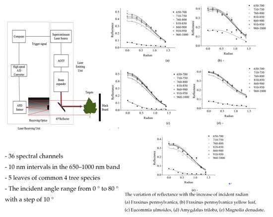
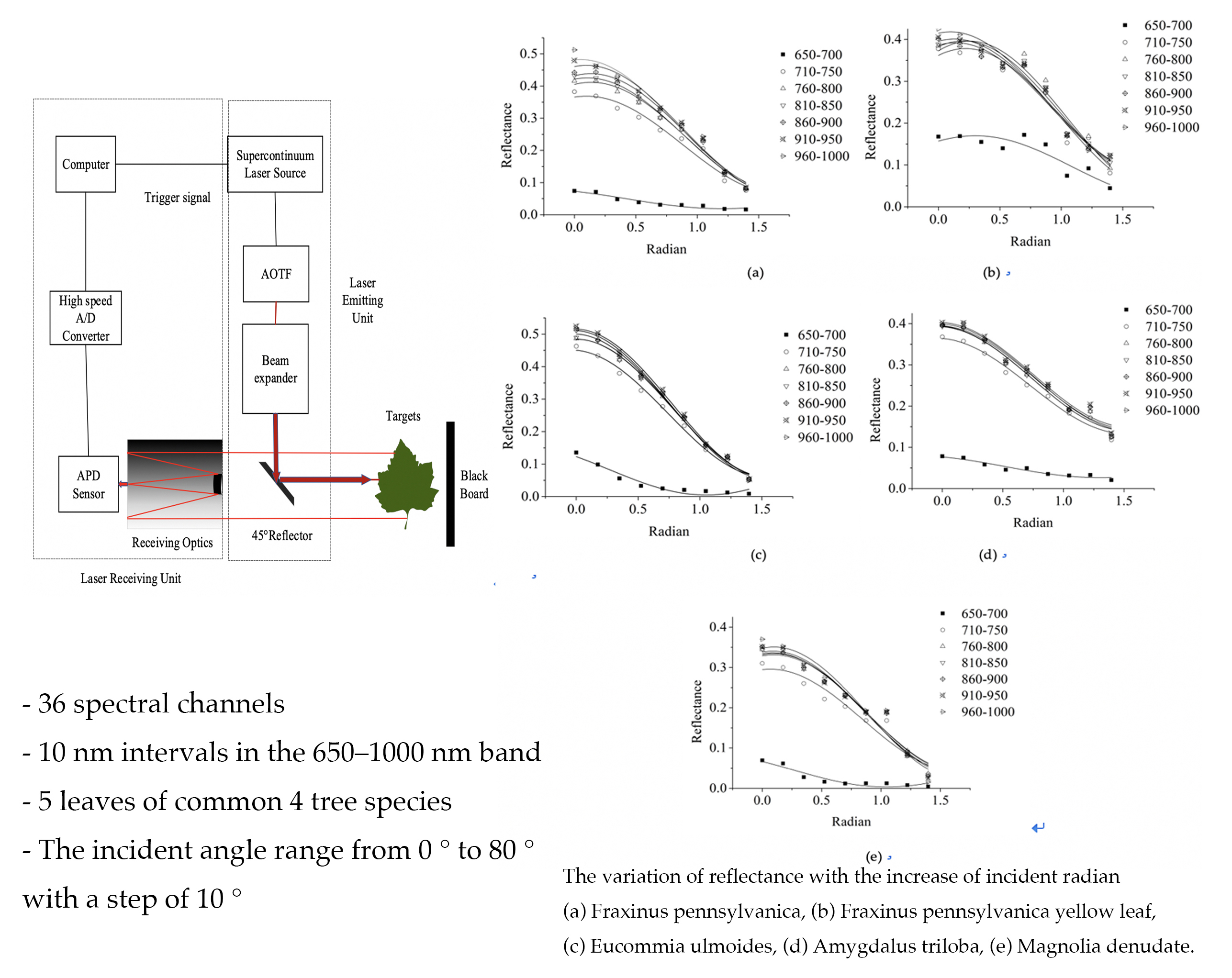
2.1.2. Hyperspectral LiDAR System

This study used a tunable hyperspectral laser system (hereinafter referred to as HSL) developed by the Institute of Optoelectronics (AOE) of the Chinese Academy of Sciences. The whole system is composed of three essential units: transmitting unit, receiving unit, and scanning control unit. To ensure that laser pulses of different wavelengths are emitted at different times as required, so that echo signals of different wavelengths are obtained at different times, the system selects a supercontinuum (SC) laser plus an acousto-optic tunable filter (AOTF) as a light source. The beam expander collimates and expands the laser light source, and is irradiated onto the detection target through a 45° mirror. The laser-receiving unit adopts a reflective receiving system, and the photodetector selects a silicon-based Avalanche Photon Diode (APD) detector with a strong effect rate in the visible and near-infrared region, which is a photosensitive element used in laser communication. The scanning control unit uses the two-dimensional turntable of the laboratory for simultaneous scanning.

The HSL laser source is based on the fiber lasers and photonic crystal fibers with a spectral band covering between 430 and 1450 nm. It can output laser pulse with a repetition rate of 0.1–200 MHz and a total power of >8 W. The single pulse energy can reach up to 19 mJ. The repetition frequency is 0.1 Mhz, the transmission power is 2 W, and the spectral width is over 1000 nm. The working wavelength is in the near-infrared region of visible light. Because of the SC laser source emitting a very weak beam within the spectrum, we do not use blue band in this experiment. The working spectrum of the red-edge region and the near-infrared region is often used; therefore, the tunable Hyperspectral LiDAR (THSL) employed in this paper works with spectral bands, covering from 650 to 1000 nm at 10 nm resolution. Therefore, with these settings, there are 36 different spectral channels in this THSL.

Figure 1 presents an illustrative diagram of the proposed AOTF-HSL system. In this system, a SC laser (Leukos © SCM 30-HE-450) is employed as a laser source which emits the supercontinuum lasers pulse with spectral wavelength ranging from 450 to 2400 nm. The SC laser firstly emits a laser beam which is collimated by a reflected fiber collimator. Then, the collimated laser beam passes through a beam sampler, which utilizes a minor part of the collimated beam for triggering time-of-flight measurement. A photodetector is employed to detect the triggering signal, and transfer the signal to a linked high-speed oscilloscope for initializing the data recording operation.

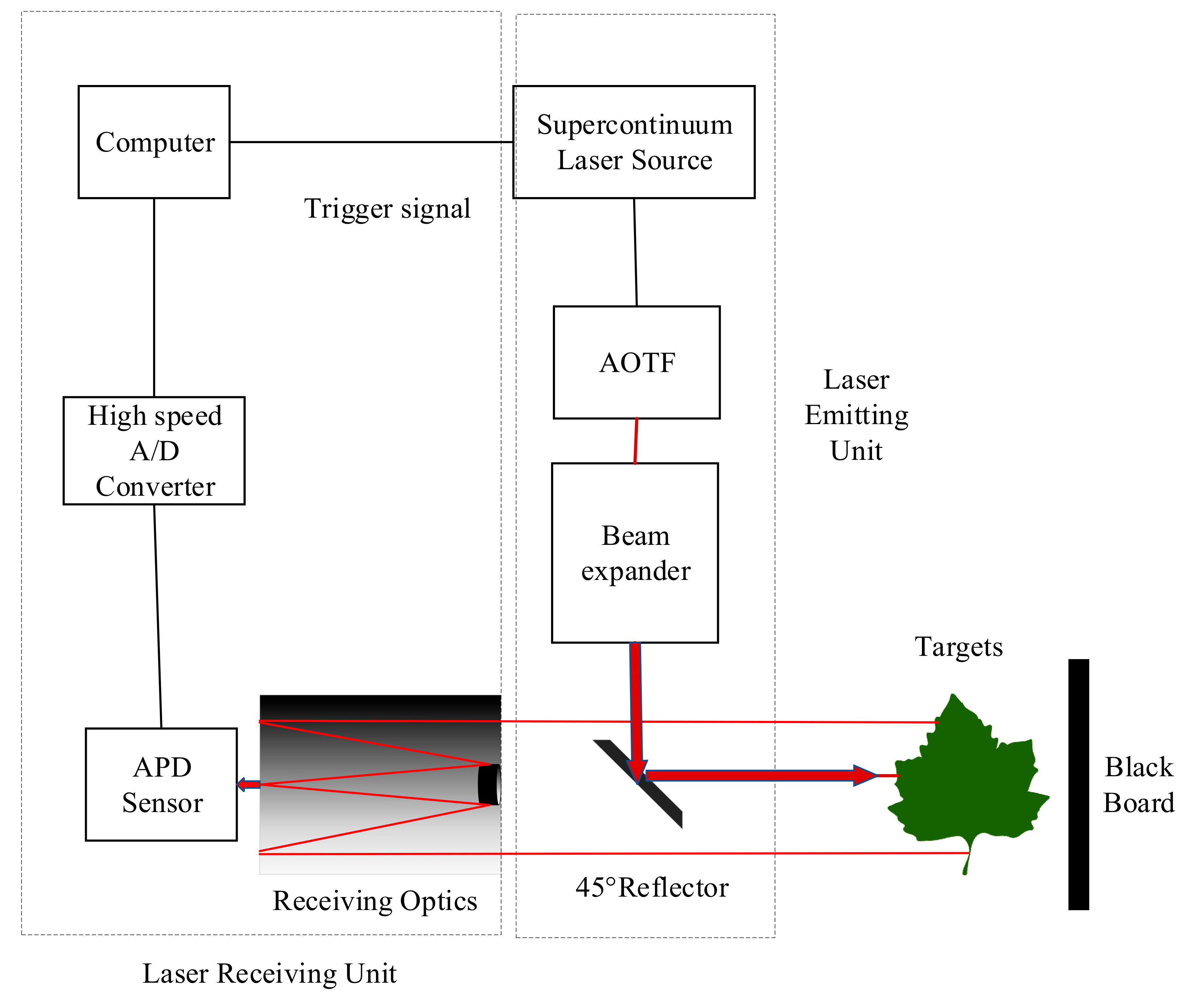
2.1.3. Hyperspectral LiDAR Measurement

The reflectance of five kinds of leaves (Fraxinus pennsylvanica, Eucommia ulmoides, Amygdalus triloba, yellow leaf of Fraxinus pennsylvanica, Magnolia denudate) was measured by the HSL. Yellow leaf is only chosen from one species (Fraxinus pennsylvanica) is based on the fact that the difference in spectral reflectance among the broad yellow leaf is small. The measurement range of the lab experiment is approximately 8.5 m away from the leaf to be measured. For each leaf, a standard reflectance white board (Spectra Vista Corporation © HR-1024) was first placed on the detection position, and the response waveform of each wavelength was detected and recorded by the HSL. The white board is produced by SVC and it’s an accessory white board of SVC HR-1024. The white board is a 100% reflectance panel and the size is 210 mm * 260 mm. Then, the leaf was placed in the same position and fixed on a blackboard, to repeat the identical measurements for each wavelength. Moreover, the blackboard is approximate blackbody, and fixed it to the turntable. By controlling the angle of the turntable, the incident angle is determined, which is ranged from 0° to 80° with a step of 10°. Assuming the reflectance of the white board is 100%, the reflectance of the leaf in a certain band is the ratio of the two waveforms. Thus, the reflectance of each leaf changed with the leaf angle was determined.

The calculation formula of leaf spectral reflectance measured by HSL is:

$$\mathsf{\rho }\left(\lambda \right)=\frac{V\left(\lambda \right)}{Vs\left(\lambda \right)}·\rho s\left(\lambda \right)$$

(1)

$\mathsf{\rho }\left(\lambda \right)$ is the reflectance of the measured leaf sample at wavelength $\lambda$, $\rho s\left(\lambda \right)$ is the reflectance of the standard white board, V(λ) is the measured waveform of the different leaves, and Vs(λ) is that from the standard white board [24]. After further Gaussian smoothing on the collected waveforms, active hyperspectral reflectance of leaves of five kinds was obtained.

The APD detector used in HSL is different from the charge coupled devices (CCD) detector of Analytica Spectra Devices (ASD) FieldSpec 4 spectrometer, which is little affected by the ambient light. Since the whole system is still under the laboratory testing stage, the effect of the dark current has not been considered yet, which is a task in our future research. The total HSL experiment observation platform is shown in Figure 2. The red dot is the laser irradiation point.

2.1.4. ASD Measurement

Active spectral data of target leaves were supplemented by ASD FieldSpec 4 spectrometer (ASD © FieldSpec 4). The reflectance data measured by ASD FieldSpec 4 spectrometer was used for the comparison of active and passive reflectance. Different from active spectral measurement, ASD observation is very efficient, so multiple measurements are made at the target site of each leaf to obtain the average spectrum and fluctuation (standard deviation). The specific measurement process is as follows:

(1) Dark current removal.

To ensure the accuracy of the measured data, the dark current value of each leaf will be re-collected before measurement. This step is automatically collected by the spectrometer itself before measurement.

(2) The whiteboard correction.

The measured spectra of the reference white board are stored in the memory of the laptop. The experiment was conducted in a dark room with constant lighting conditions. Halogen lamps were used to provide stable light source. White board reference was collected every 10–15 minutes during the preheating phase of the instrument. Finally, ViewSpec Pro, the spectral data processing software of the spectrometer, can facilitate the acquisition of reflectance data of target objects. In the experiment, the reflectance of leaf and white board is calculated by the signal value, and the reflection curve is smoothed by ViewSpec Pro.

(3) Fifteen repeated measurements were made at different positions of the leaves.

In order to avoid spectral differences caused by different physiological and biochemical parameters at different positions of leaves, the spectrum of leaves was measured at the target position of leaf flesh in this experiment, and each leaf was repeated for 15 times.

The spectral reflectance of leaves measured by FieldSpec 4 surface feature spectrometer was preprocessed with ViewSpec Pro to obtain the spectral reflectance curve corresponding to leaves.

In order to facilitate the comparison of active and passive spectra, the passive spectral curves were resampled according to the HSL band. A total of 36 spectral channels at 10 nm intervals in the 650–1000 nm band are selected as the target band. The passive hyperspectral curve observation platform is shown in Figure 3.

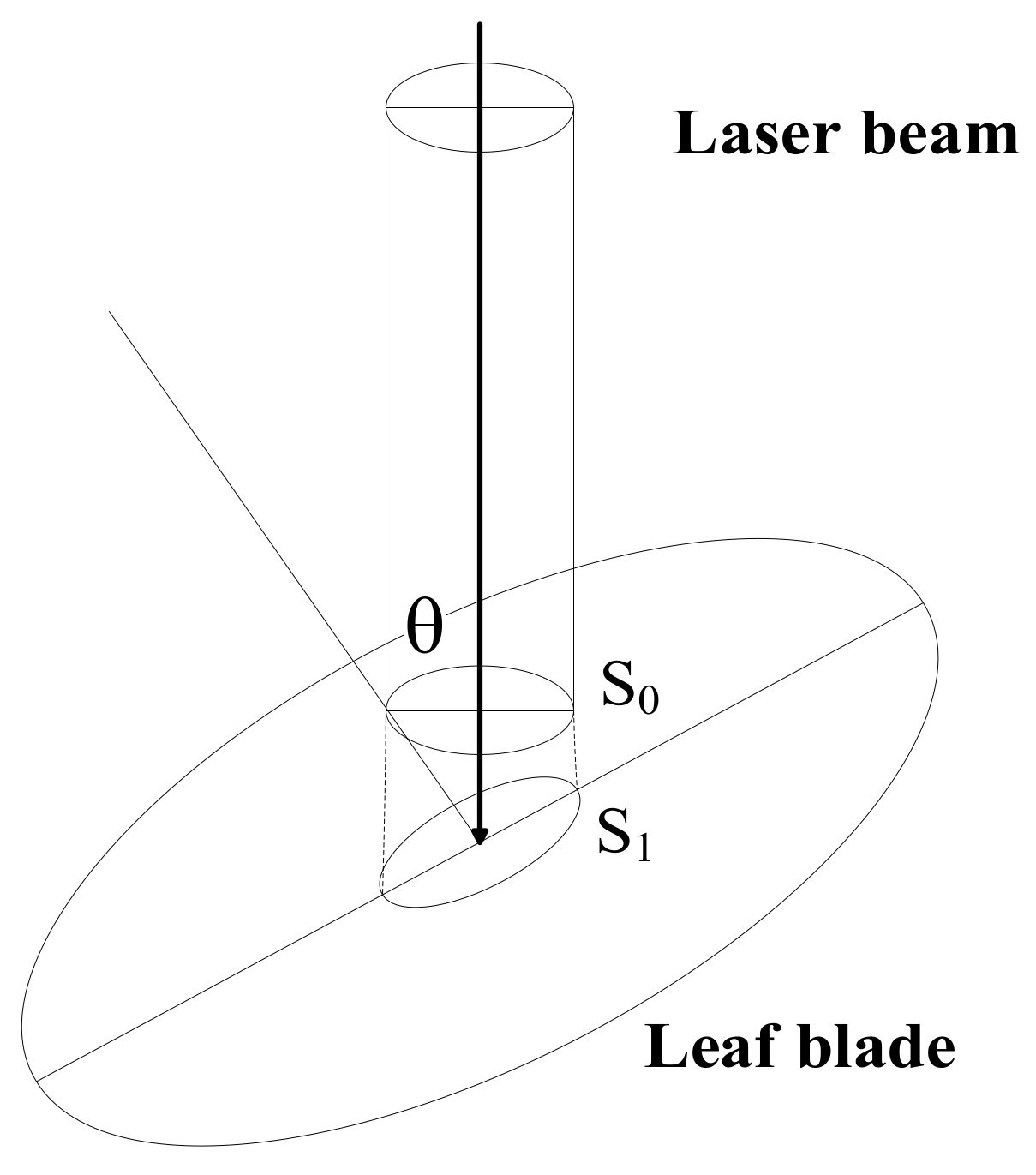
2.2. Angle Effect Modelling

In the experiment, the theta angle of the leaf is the included angle between the laser incident direction and the normal direction of the leaf, and the center of the laser spot on the leaf is the fixed incident point, so as to control the same parts of the leaf to be tested. At the same time, nine gradients of leaf inclination were set, respectively: 0°, 10°, 20°, 30°, 40°, 50°, 60°, 70°, and 80°. The leaf incidents were measured by the compass.

However, we derived the radiant flux density of the leaf here step by step because we use a formulation particularly adapted to HSL, and it provides the basis for our further considerations. The main parameters involved in the LiDAR equation are illustrated in Figure 4. The laser transmits a narrow beam towards the scatterer [25].

All target parameters were combined into one parameter, the so-called backscatter cross-section σ:

$$\mathsf{\sigma }=\frac{4\pi }{\mathsf{\Omega }}{\rho }_{\theta }{A}_s$$

(2)

where ${\rho }_{\theta }$ is the bidirectional reflectance distribution function (BRDF) when the incident angle and the exit angle are both θ, and A_s is the receiving area of the scatterer. The reradiation pattern is in general complex [26], but for simplicity, we assume that the incoming radiation is scattered uniformly into a cone of solid angle Ω [25].

According to the constant laser emission energy, we assume that the laser emission power is P, the radiant flux density is E, the laser beam vertical projection leaf area is S₀, and the leaf inclination angle is θ, then:

$$\mathrm{E}=\frac{\mathrm{P}}{S_{0}cos\mathsf{\theta }}$$

(3)

It can be concluded that the relationship between the radiant flux density E₀ of the leaf and the radiant flux density E of the leaf under different leaf inclination angles, under the condition of vertical laser incident leaf inclination is:

$${\mathrm{E}}_{\mathrm{0}}=\mathrm{E}·cos\mathsf{\theta }$$

(4)

Using the method of orthogonal regression design, the same leaf reflectance R establishes a three-dimensional model with the relationship between the leaf inclination angle θ and the wavelength λ, which is a nonlinear binary quadratic system and established by interpolation. Moreover, the model is:

$$R=z_0+a\times \theta +b\times \mathsf{\lambda }+\mathrm{c}\times {\mathsf{\theta }}^2+d\times {\mathsf{\lambda }}^2+f\times \theta \times \mathsf{\lambda }$$

(5)

where $z_0$, a, b, c, d, and f are constants.

At the same time, the whole band is decomposed into seven bands of 650–700 nm, 710–750 nm, 760–800 nm, 810–850 nm, 860–900 nm, 910–950 nm, 960–1000 nm, and a reflectance R is established for each band:

$$\mathrm{R}=\mathrm{ACos}\left(\mathsf{\theta }-{\mathsf{\theta }}_0\right)$$

(6)

where A and ${\mathsf{\theta }}_0$ are constants.

Meanwhile, the normalized value of reflectance R_N in Near Infrared (NIR) (710–1000 nm) and Red (650–700 nm) are calculated respectively in order to explore how they change with the increase of incident angle:

$$R_N=\frac{R_{\theta }}{R_0}$$

(7)

where $R_{\theta }$ is the reflectance measured by HSL when the incident angle is $\mathsf{\theta }$, and $R_0 is$ the reflectance measured in 0°.

3. Results

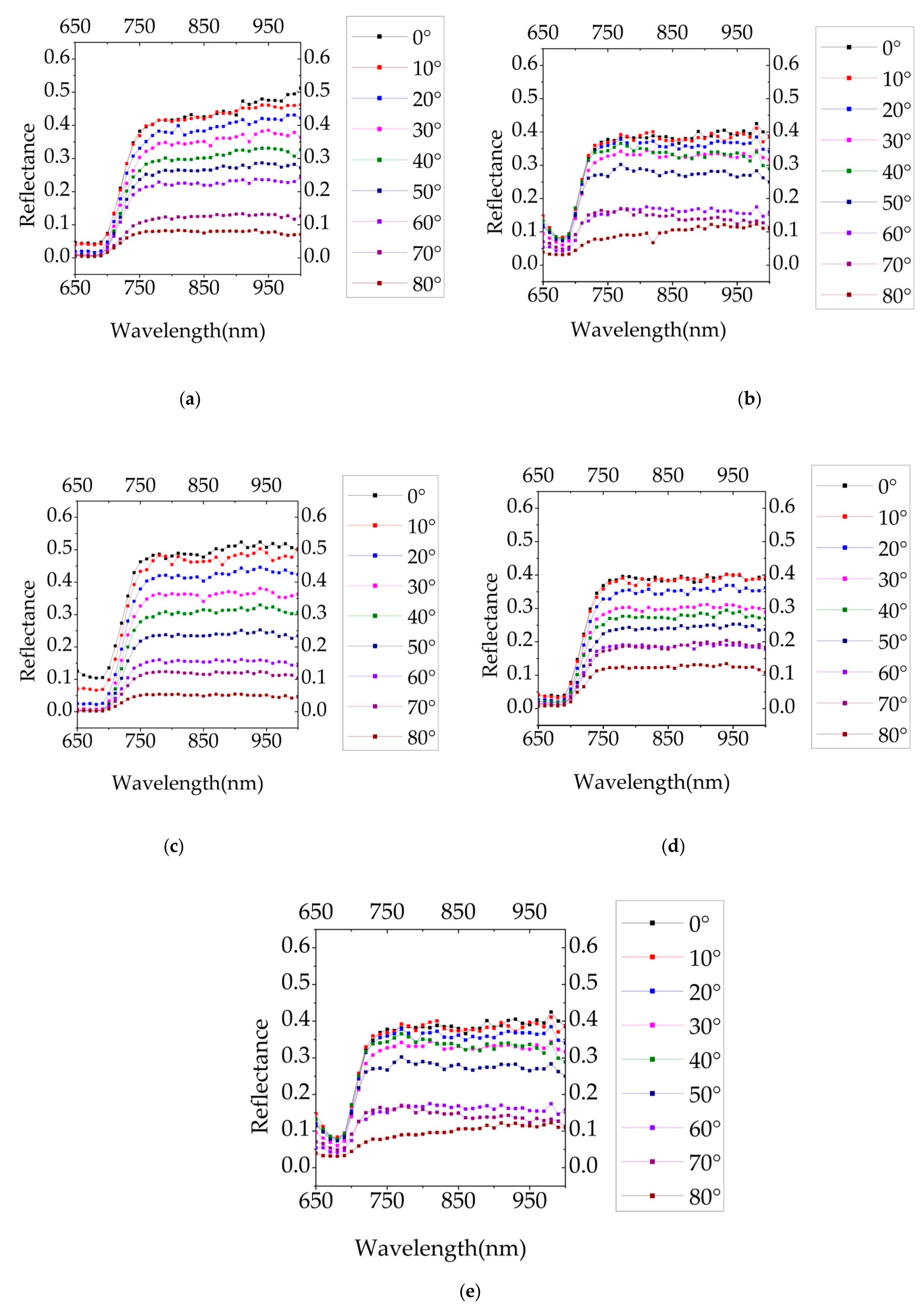
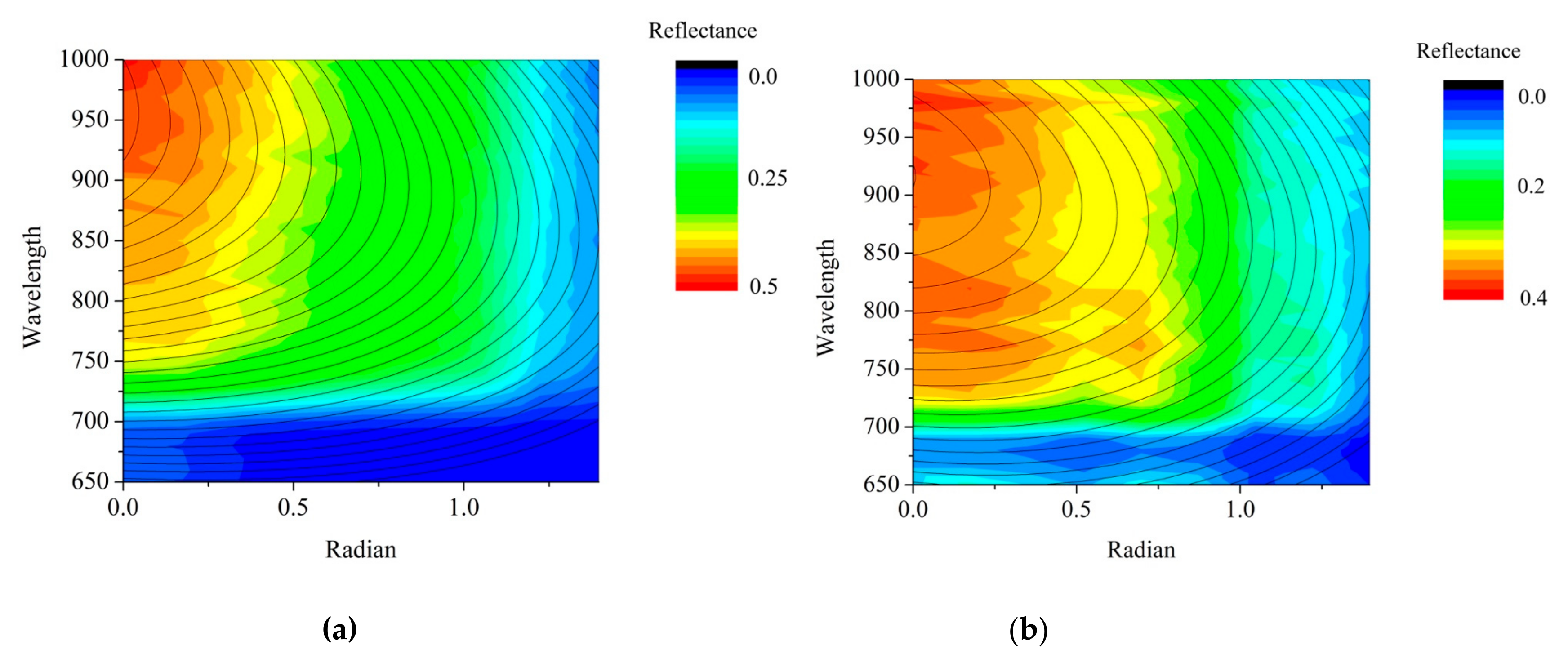
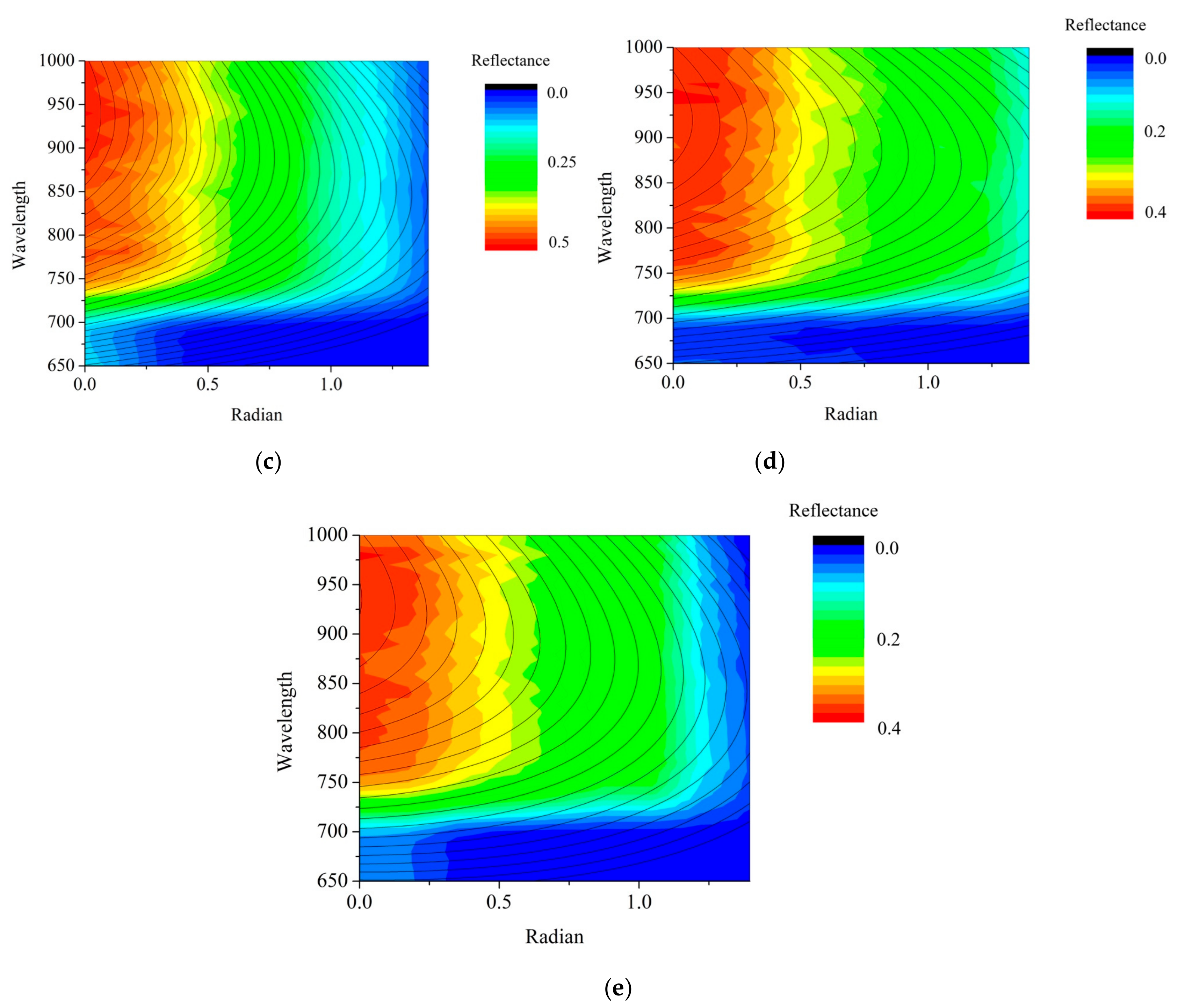
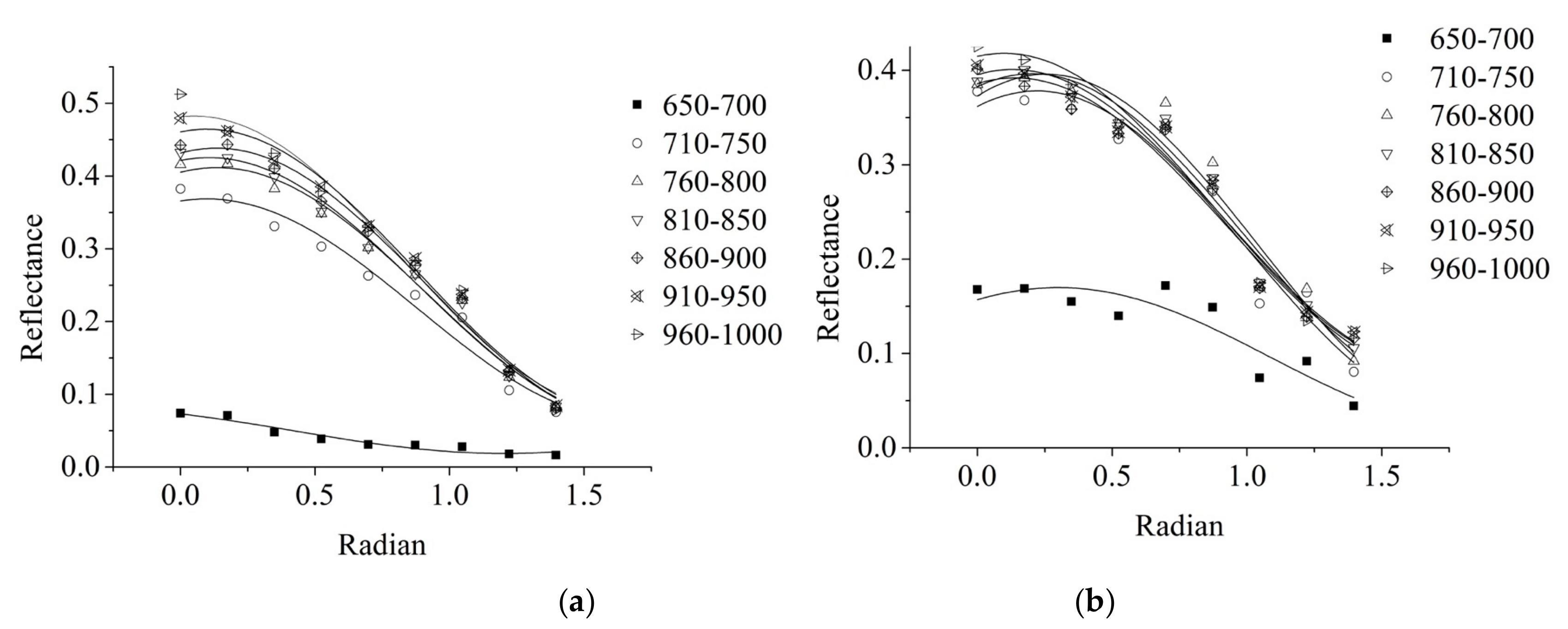
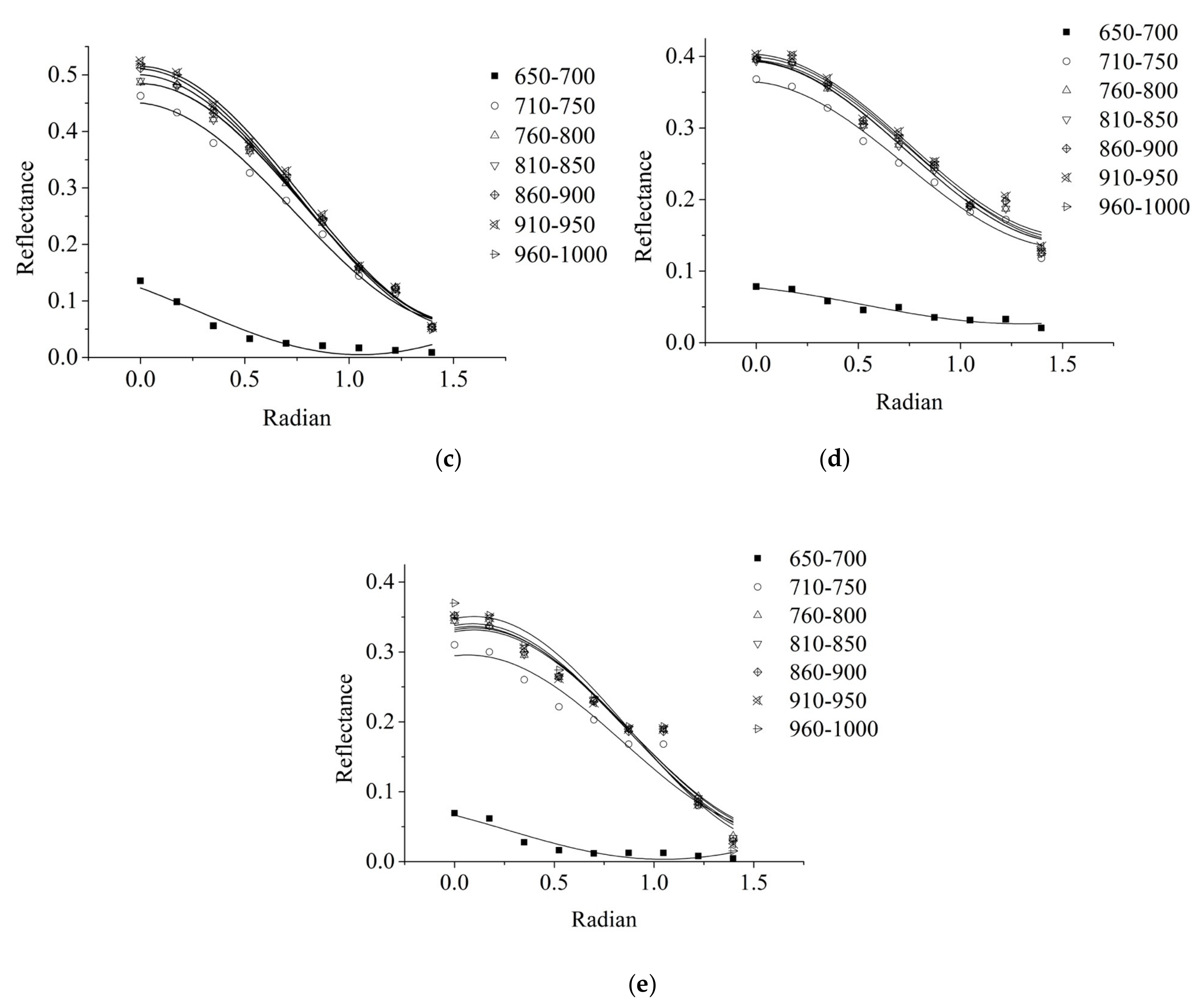
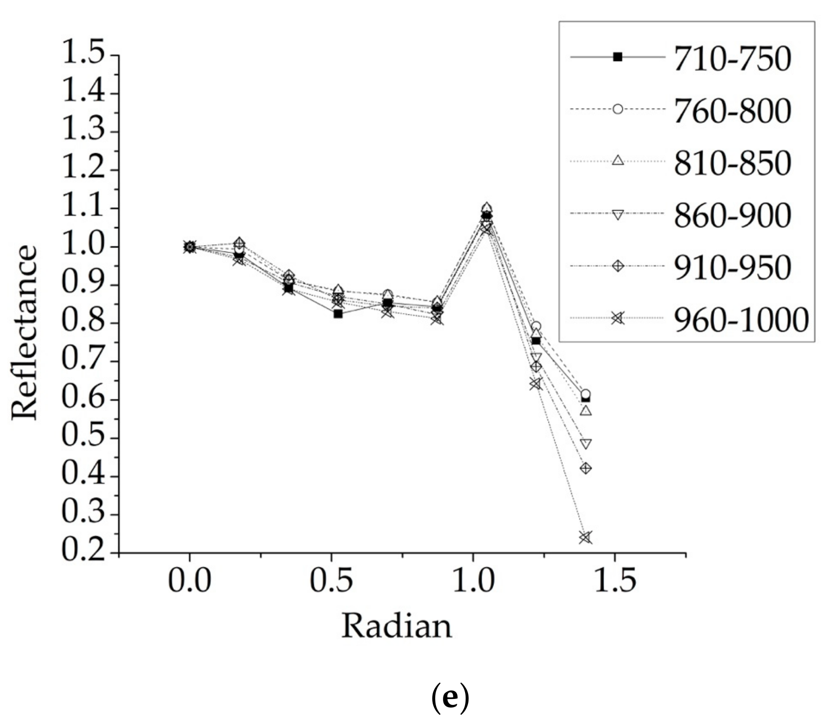
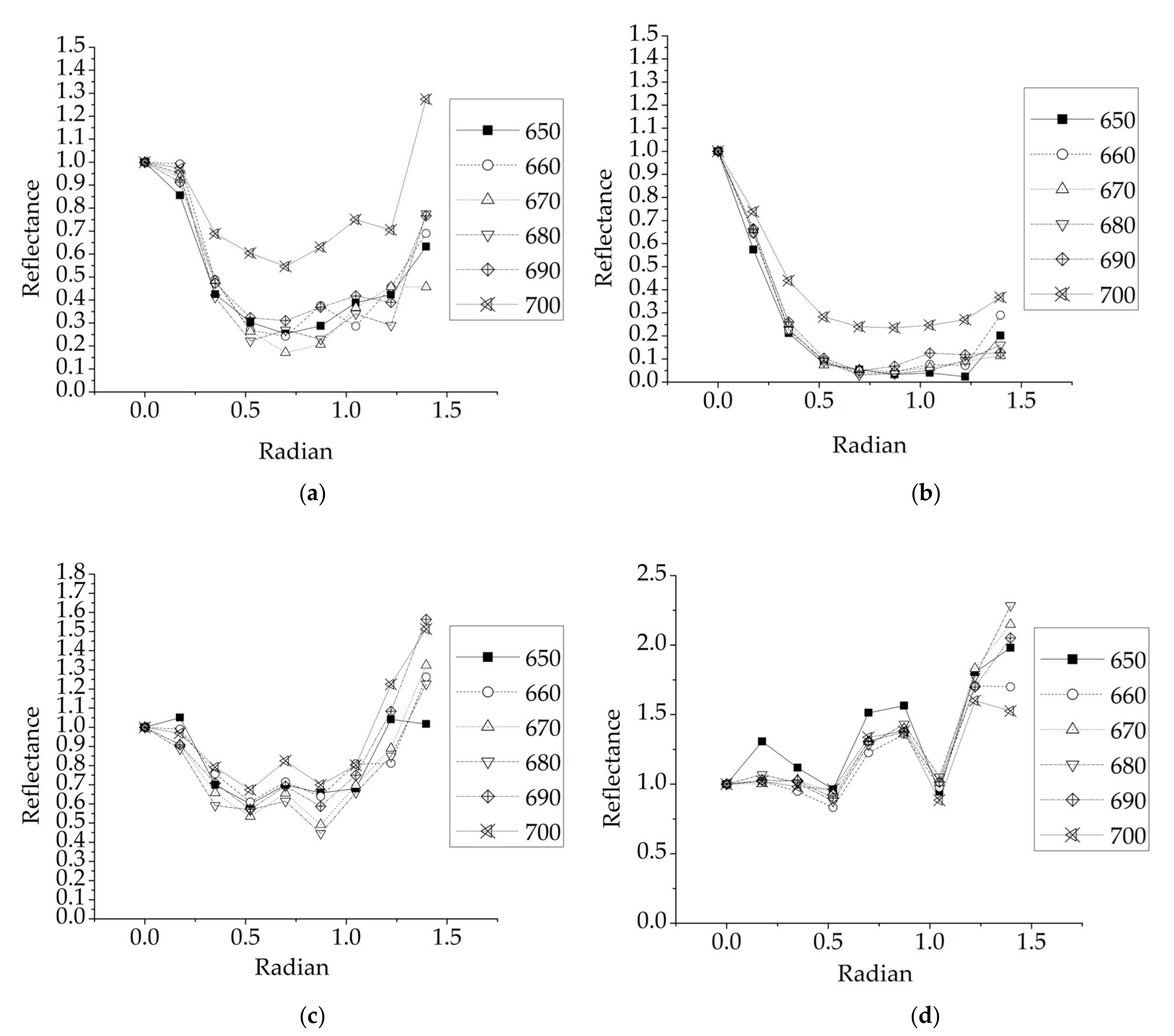
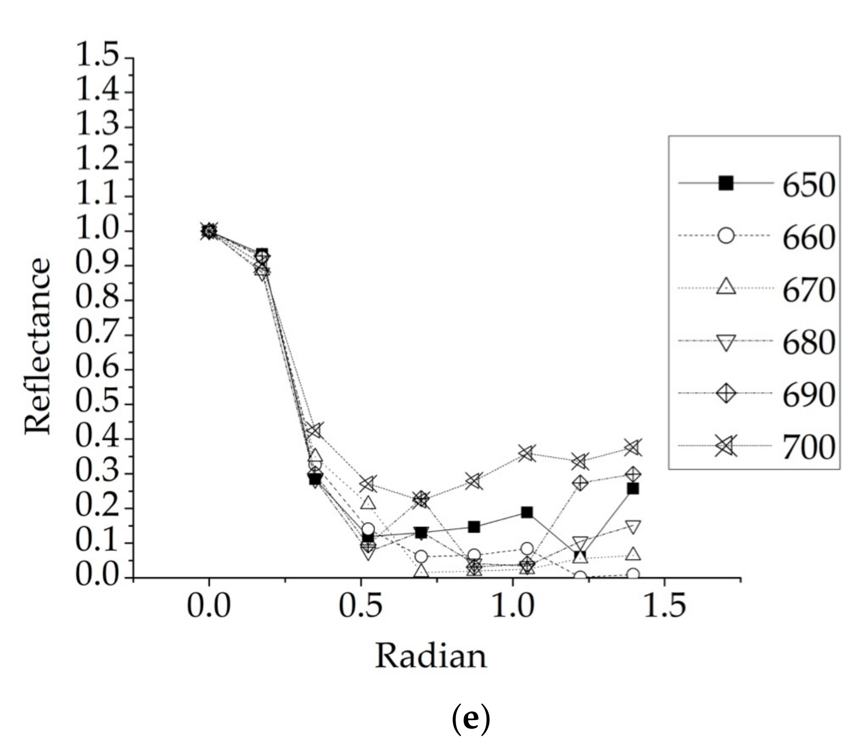
3.1. Reflectance under Different Leaf Obliquity

Figure 5 shows the spectral curves of 36 bands of the five different leaves measured by the HSL at different leaf inclinations. It can be seen that the spectral curve of green leaves is low in the visible region and high in the near-infrared region, with obvious red edges, which conforms the spectral characteristics of vegetation leaves. In the process of increasing leaf inclination angle, the reflectance of the leaf also decreases with the change of angle. There is a distinguished difference between yellow ash leaf and green leaf in visible band.

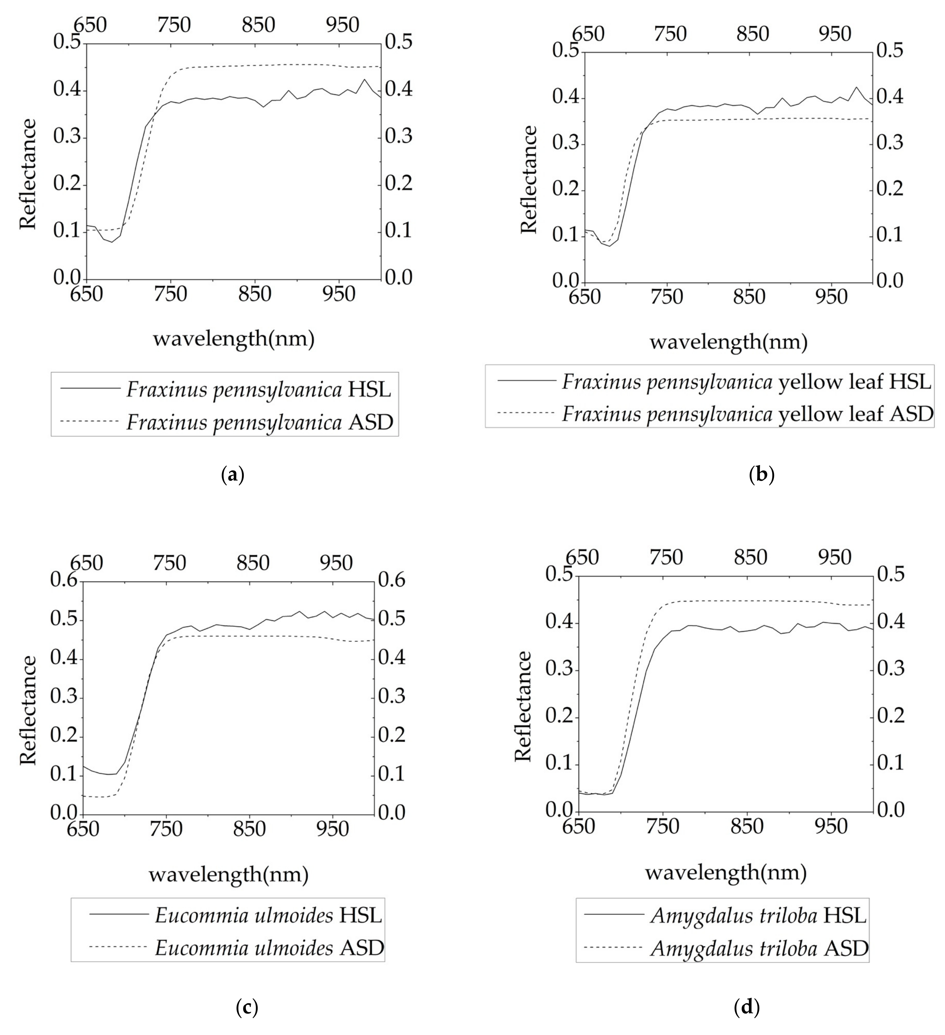
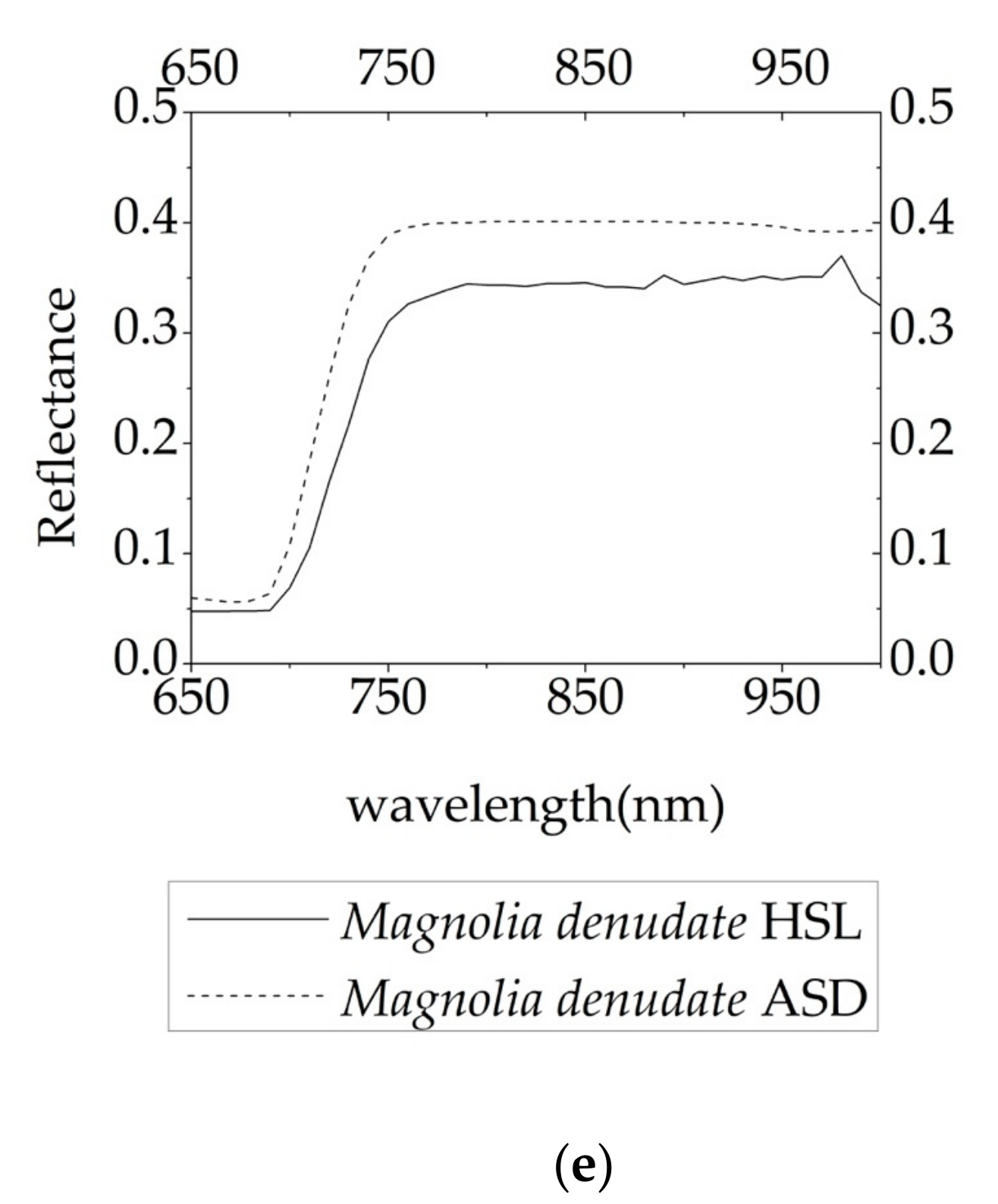
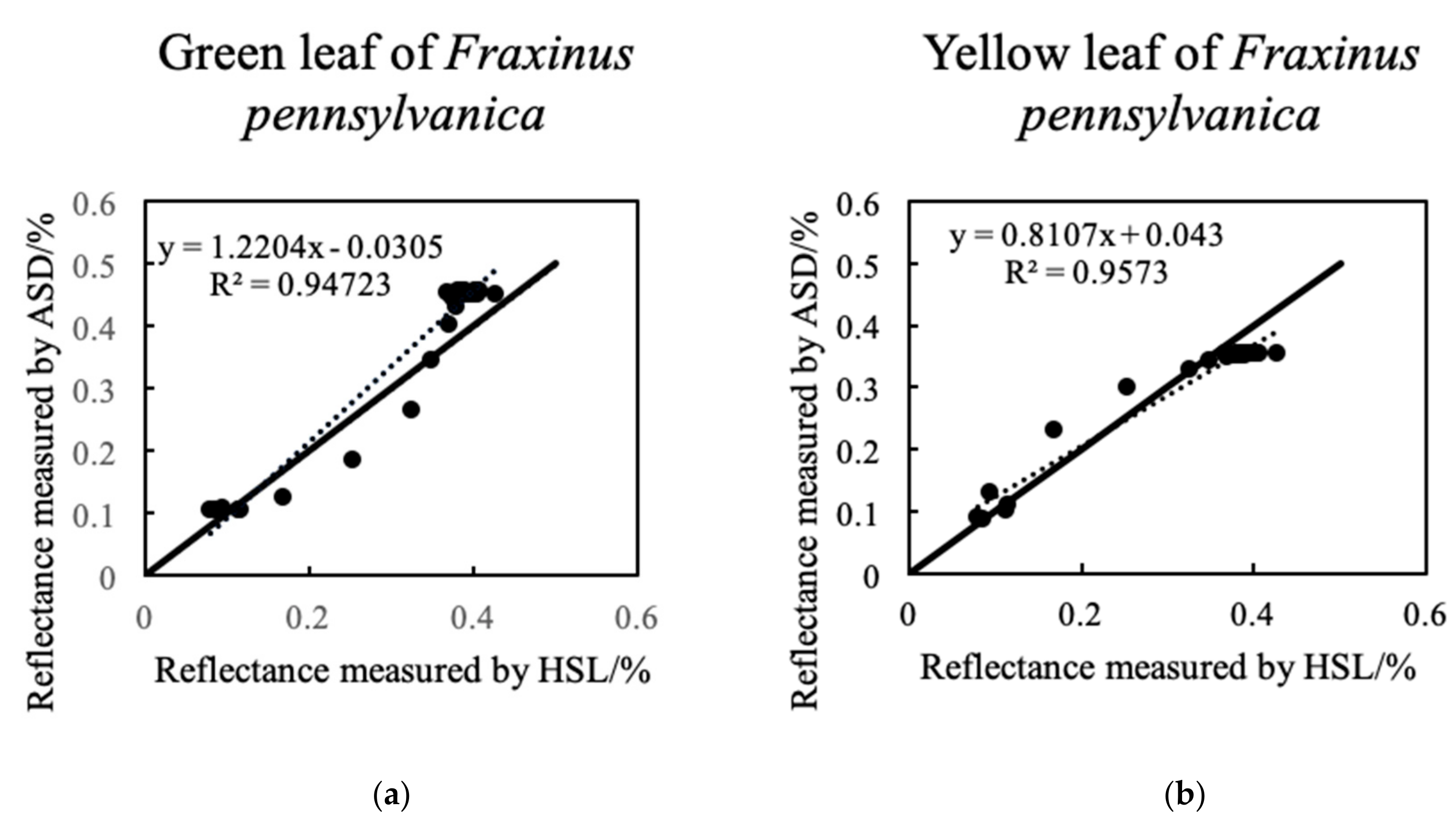
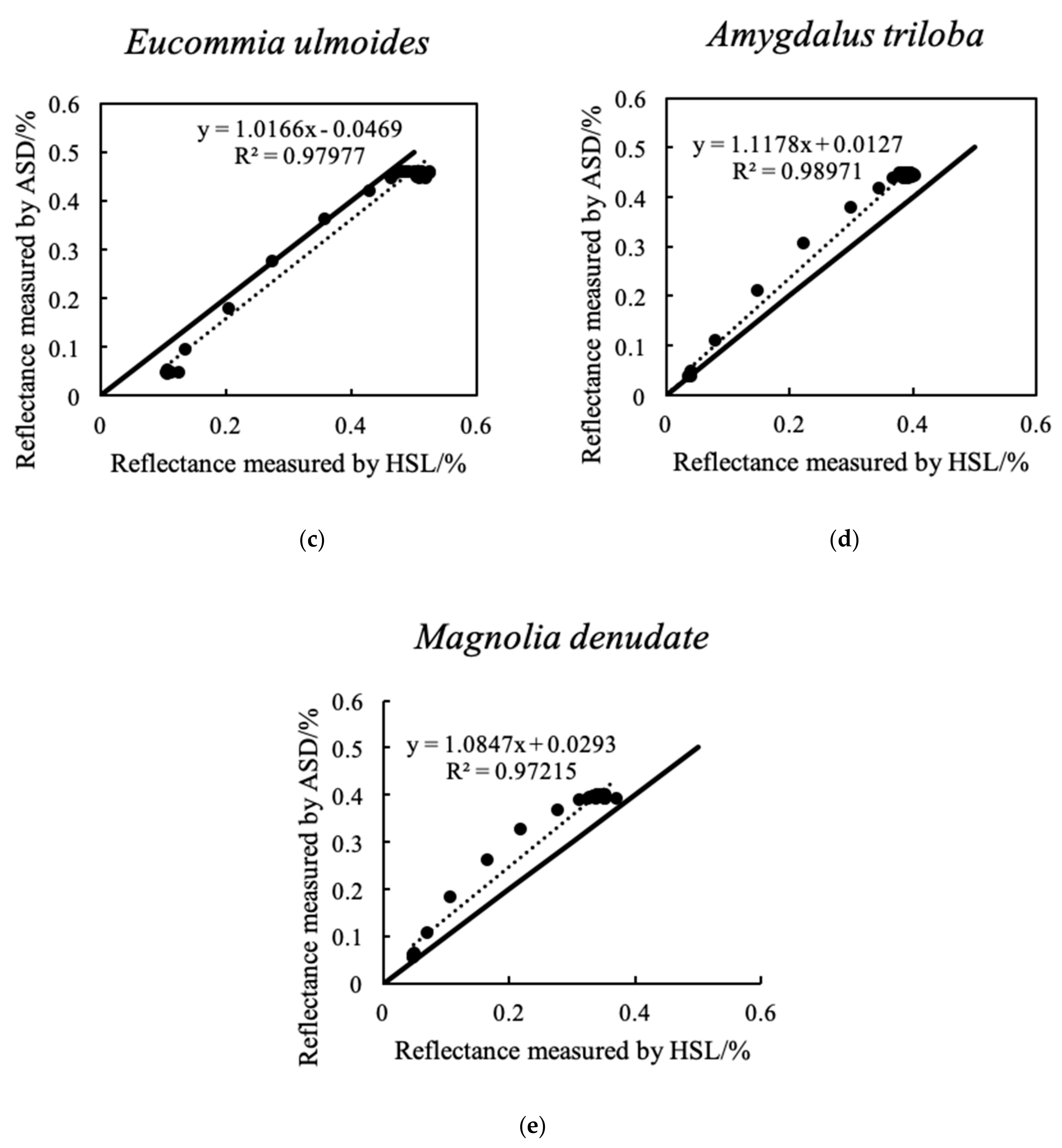
3.2. HSL vs. ASD Measurements

Figure 6 shows the comparison between the data measured by hyperspectral LiDAR and the data measured by ASD FieldSpec 4 spectrometer. Moreover, we find that the reflectance similarity between different instruments is very high. Since we mainly study the angle effect of the hyperspectral LiDAR in the spectral range between 650 and 1000 nm, only the ASD FieldSpec 4 spectrometer data in the same band is selected for comparison, and other data were not included in the comparison.

We computed the distributions of the reflectance from the green leaves of the five plants from the hyperspectral LiDAR, compared them with the reflectance determined by the spectrometer data, and present the scatterplots of the reflectance from AOTF-HSL versus that from the ASD spectrometer in Figure 7 with a linear fit. High coefficients of determination (R² > 0.94) in all five cases indicate that the extracted reflectance from HSL highly correlates with the ASD. For the five green leaf cases, the average value is close to 0.9692, which demonstrates the excellent fitness of the measurements from the two devices. It can be preliminarily concluded that the reflectance result of the HSL system using the proposed calibration method are reliable.

3.3. Leaf Angle Model

3.3.1. Construction of Leaf Reflectance Model

In this experiment, a reflectance R is established for each leaf. A leaf reflectance model is established with the relationship between the leaf inclination angle θ and the wavelength λ. Meanwhile, we calculate and compare their Root Mean Square (RMS) and the coefficient of determination (R²).The model parameters and the accuracy are shown in

Table 2. The parameters of 5 leaf three-variable model.

	${\mathbf{z}}_0$	a	b	c	d	f	RMS	R2
Green leaf of Fraxinus pennsylvanica	−4.312	0.559	0.010	−0.083	−5.247E-6	−7.979E-4	0.002	0.931
Yellow leaf of Fraxinus pennsylvanica	−3.191	0.356	0.008	−0.121	−4.295E-6	−4.543E-4	0.002	0.869
Eucommia ulmoides	−4.434	0.426	0.011	−0.016	−5.593E-6	−8.240E-4	0.002	0.929
Amygdalus triloba	−4.092	0.261	0.010	−0.015	−5.321E-6	−4.831E-4	0.001	0.904
Magnolia denudate	−3.527	0.400	0.008	−0.060	−4.462E-6	−5.999E-4	0.001	0.912

.

It can be seen that for the leaves with different roughness (smooth leaves, such as M. denudate; rough leaves, such as A. triloba), the absolute value of the a parameter of the Yellow leaf of F. pennsylvanica and A. triloba is slightly lower, while the parameter a of M. denudate and Green leaf of F. pennsylvanica is slightly higher. The parameter a has a certain correlation with the roughness of the leaf, indicating that the leaf angle effect has different degrees of influence on different leaf roughness. The rougher the leaf surface, the smaller the effect of the angle effect on the reflectance, otherwise the smoother the leaf surface, the greater the effect of the angle effect. For leaves with lower greenness (F. pennsylvanica yellow and M. denudate leaves), the parameters b and d have smaller absolute values, while absolute values in Green leaf of F. pennsylvanica, E. ulmoides, and A. triloba leaves with greater greenness are larger. It shows that the wavelength has different effects on the reflectance for leaves with different greenness.

Figure 8 illustrates the model of reflectance changing with leaf obliquity and wavelength, which is established by interpolation method. Based on the incident angle data and the wavelength, we can simulate the leaf reflectance correspondingly. Although the Root Mean Square (RMS) are all small, the model fitting degrees of the four green leaves are higher than that of the F. pennsylvanica yellow leaves. In addition, it can be observed that the reflectivity of both green leaves and yellow leaves decrease with the increase of incident angle when the wavelength is unchanged. When the incident angle remains unchanged, the reflectance of green leaves decreases with the decrease of the wavelength, while the F. pennsylvanica yellow leaves still have some unstable fluctuations.

3.3.2. Echo Intensity Changing with Incident Angle

In order to investigate echo intensity changing with incident angle, this experiment decomposes the whole band into seven discrete bands: 650–700 nm, 710–750 nm, 760–800 nm, 810–850 nm, 860–900 nm, 910–950 nm, 960–1000 nm. The maximum values of each band changed with the leaf angle are shown in Figure 9.

It can be seen from Figure 9 that as the wavelength increases, the reflectance also increases. All green leaves show a consistent pattern.

Table 3. The parameters of Leaf reflectance models and the corresponding accuracy.

		A	${\mathsf{\theta }}_0$	RMS	R2
650–700	Green leaf	0.06926	−0.21696	0.01285	0.55284
	Yellow leaf	0.16883	0.14514	0.00286	0.81485
710–750	Green leaf	0.35832	−0.03303	0.00173	0.85779
	Yellow leaf	0.37960	0.04701	0.00074	0.93966
760–800	Green leaf	0.39642	−0.02874	0.00179	0.87742
	Yellow leaf	0.039669	0.06901	0.00083	0.93660
810–850	Green leaf	0.40019	−0.03422	0.00183	0.87861
	Yellow leaf	0.39598	0.05686	0.00050	0.96074
860–900	Green leaf	0.40850	−0.03593	0.00220	0.86267
	Yellow leaf	0.38819	0.04845	0.00059	0.9514
910–950	Green leaf	0.42176	−0.04285	0.00265	0.84906
	Yellow leaf	0.39585	0.05144	0.00063	0.94911
960–1000	Green leaf	0.42685	−0.05959	0.00251	0.86301
	Yellow leaf	0.41143	0.02694	0.00065	0.95381

shows that in the 710–1000 nm band, the model has a high degree of fit.

Because there are some differences in the spectral curves of green leaves and yellow leaves, this experiment grouped F. pennsylvanica, E. ulmoides, A. triloba, and M. denudate into green leaves to model while the yellow leaf of F. pennsylvanica is modeled as yellow leaf separately in the modeling process.

The fitting result is relatively good in Table 3. In the NIR band (710–1000 nm), the R² of the model fitted by the green leaves are all higher than 0.85, while that of the model fitted by the yellow leaves are higher than 0.93. However, in the RED band (650–700 nm), the R² of the yellow leaves is higher at 0.81, while that of the green leaves is relatively lower at 0.55.

The phenomenon observed by Figure 10 and Figure 11 confirms the results below. It can be seen from Figure 10 that in NIR (710–1000 nm), the curve of all four species green leaves is relatively smooth in the range of 0–0.8 radians. In contrast, F. pennsylvanica yellow leaf keeps decreasing in this range. In the radian range of 0 to 0.8, the curves of all leaves show relatively severe fluctuations. Figure 11 shows that in RED (650–700 nm), the curve of all the leaves except A. triloba decrease in the range of 0–0.8 radians, and gradually increase in the range upper 0.8 radians. Oppositely, there are two reflection valleys of A. triloba in the red wave band, which fluctuate wildly in the whole angle range. After the incident correction, in the near-infrared band (710–1000 nm), all four green leaves exhibit Lambert in the radian range of 0 to 0.8, which the normalized value of reflectance tends to be 1 at a stable level. However, for the yellow leaf of F. pennsylvanica, the normalized value of reflectance has a tendency of declination. Moreover, all the leaves exhibit severe jitter in the radian above 0.8. In the red band (650–700 nm), the leaf exhibits a distinct non-Lambertian feature, and the normalized reflectance value decreases with increasing angle after incidence correction in the radian range of 0 to 0.8.

4. Discussion

This paper studies the angle effect of leaf reflectance measured by a continuous hyperspectral LiDAR, which is seldom studied before. Through this study, we can determine the leaf inclination angle, according to the corresponding laser wavelength and the reflectance obtained by the measurement. Previous studies only focused on the reflectance of hyperspectral LiDAR in single-wavelength or multi-wavelength, and no further studies were conducted on the different characteristics of leaves. Moreover, in this research, it can be extended from the single leaf scale to single tree scale and even to the plot scale. The hyperspectral LiDAR itself can obtain the reflectance of the leaf at different wavelengths with high spectral resolution. After establishing the correction model, the leaf angle of the target leaf can be directly obtained by the wavelength and the reflectance. Furthermore, the leaf reflectance of the incident angle can be corrected to perpendicular incident direction, and then more applications, such as the classification of the leaf, the separation of the branches from wood, etc., can be conducted.

Although the results are preliminary, they suggest that the use of hyperspectral LiDAR for laser scanning of the leaf must consider factors, such as the leaf surface properties and internal structures. In the future, when measuring real and complex targets, such as a tree, the laser hits more than one leaf or one needle, multiple echoes are generated. The curvature of the leaves, the angular distribution, and the irregularities of other shapes are likely to average the effect of the angle of incidence, at least on the scale of the entire tree. However, this must be better described in future experiments, especially in the red and near-infrared spectral regions.

In this paper, the relationship between the reflectance of the hyperspectral LiDAR and the incident angle is explored. The specular reflection is significant in the red band, and it has obvious non-Lambertian characteristics. Obvious bowl edge effect and the white wax with smooth surface can be observed. This appearance of specular reflection in Magnolia denudate is particularly obvious; in the near-infrared, no specular reflection occurs, but Lambertian characteristics are present. This is similar to the results of the study conducted by Balduzzi (Balduzzi and Van der Zande et al., 2011) using a 785 nm laser. We studied the leaves with different surface properties and internal structures and explored the role of specular reflection in different parts of the spectrum. The results show that for smooth surfaces such as ash and magnolia, specular reflection is obvious in both red and near-infrared regions. Among them, leaves with larger leaf thickness, such as magnolia, have relatively strong specular reflection throughout the entire band.

During the experiment, the spot has a certain size. When the leaf inclination angle is large, it is difficult to ensure that the incident laser is completely irradiated on the leaf area. Therefore, in the radian above 0.8, the normalized correction is performed. The reflectance value shows a phenomenon in which the fluctuation fluctuates greatly. This phenomenon also has similar results in the experimental results of Sanna Kaasalainen (Kaasalainen and Nevalainen et al. 2016). Therefore, the exploration of the angle effect of the larger leaf angle (in the radian above 0.8) can only be accurately explored by reducing the laser spot size.

This experiment used mature fresh leaves in healthy condition, without considering the influence of health, stress and maturity stage. In the future, we will continue to explore the leaf reflectance affected by the Angle under different circumstances.

5. Conclusions

The spectra of a variety of different leaf incidents were studied by a hyperspectral LiDAR. It was found that the measured spectral reflectance of the leaves by the HSL changes with different incident angle, and the three-variable model of the leaf reflectance changed with the leaf angle and wavelength is established. Solve the problem of the angle effect of the future hyperspectral LiDAR when measuring the leaf. These results require a more extensive study of the reflectance of different types of leaves at different angles for hyperspectral LiDAR to better understand the sensitivity of different surface properties and internal structure of the leaf to changes in light distribution. In the future, hyperspectral LiDAR scanning technology will be able to obtain the three-dimensional distribution of physiological and biochemical parameters of the target vegetation by means of hyperspectral laser scanning. Therefore, in order to better understand the influence of the angle effect on the vegetation reflectance, the model is used to eliminate the phenomenon of measuring the difference of the vegetation spectrum by the incident angle, so that the orthophoto spectrum of each measurement site can be accurately mapped to on a whole tree level, not just a single leaf. Future research will include more leaf types and scattering within the canopy, using appropriate leaf scattering models to simulate the interaction of the laser with the vegetation canopy.

References

1. Li, W.; Jiang, C.; Chen, Y.; Hyyppa, J.; Tang, L.; Li, C.; Wang, S.W. A Liquid Crystal Tunable Filter-Based Hyperspectral LiDAR System and Its Application on Vegetation Red Edge Detection. IEEE Geosci. Remote Sens. Lett. 2018, 16, 291–295. [Google Scholar] [CrossRef]
2. Melgani, F.; Bruzzone, L. Classification of hyperspectral remote sensing images with support vector machines. IEEE Trans.Geosci. Remote Sens. 2004, 42, 1778–1790. [Google Scholar] [CrossRef] [Green Version]
3. Camps-Valls, G.; Bruzzone, L. Kernel-based methods for hyperspectral image classification. IEEE Trans. Geosci. Remote Sens. 2005, 43, 1351–1362. [Google Scholar] [CrossRef]
4. Sun, J.; Shi, S.; Gong, W.; Yang, J.; Du, L.; Song, S.; Chen, B.; Zhang, Z. Evaluation of hyperspectral LiDAR for monitoring rice leaf nitrogen by comparison with multispectral LiDAR and passive spectrometer. Sci. Rep. 2017, 7, 40362. [Google Scholar] [CrossRef]
5. Brodu, N.; Lague, D. 3D terrestrial lidar data classification of complex natural scenes using a multi-scale dimensionality criterion: Applications in geomorphology. ISPRS J. Photogramm. Remote Sens. 2012, 68, 121–134. [Google Scholar] [CrossRef] [Green Version]
6. Næsset, E.; Kland, T. Estimating tree height and tree crown properties using airborne scanning laser in a boreal nature reserve. Remote Sens. Env. 2002, 79, 105–115. [Google Scholar] [CrossRef]
7. Juan, F.D.; William, C.; Craig, G.; Ramesh, S.; Zhigang, P.; Nima, E.; Abhinav, S.; Darren, H.; Michael, S. Capability Assessment and Performance Metrics for the Titan Multispectral Mapping Lidar. Remote Sens. 2016, 8, 936. [Google Scholar]
8. Chen, Y.; Räikkönen, E.; Kaasalainen, S.; Suomalainen, J.; Hakala, T.; Hyyppä, J.; Chen, R. Two-channel Hyperspectral LiDAR with a Supercontinuum Laser Source. Sensors 2010, 10, 7057–7066. [Google Scholar] [CrossRef] [Green Version]
9. Wang, L. Estimation of leaf biochemical content using a novel hyperspectral full-waveform LiDAR system. Remote Sens. Lett. 2014, 5, 693–702. [Google Scholar]
10. Kaasalainen, S.; Nevalainen, O.; Hakala, T.; Anttila, K. Incidence Angle Dependency of Leaf Vegetation Indices from Hyperspectral Lidar Measurements. Photogramm. Fernerkund. Geoinf. 2016, 2016, 75–84. [Google Scholar] [CrossRef]
11. Luo, S.; Cheng, W.; Xiaohuan, X.; Hongcheng, Z.; Dong, L.; Shaobo, X.; Pinghua, W. Fusion of Airborne Discrete-Return LiDAR and Hyperspectral Data for Land Cover Classification. Remote Sens. 2016, 8, 3. [Google Scholar] [CrossRef] [Green Version]
12. Bork, E.W.; Su, J.G. Integrating LIDAR data and multispectral imagery for enhanced classification of rangeland vegetation: A meta analysis. Remote Sens. Env. 2007, 111, 11–24. [Google Scholar] [CrossRef]
13. Hakala, T.; Suomalainen, J.; Kaasalainen, S.; Chen, Y. Full waveform hyperspectral LiDAR for terrestrial laser scanning. Opt. Express. 2012, 20, 7119. [Google Scholar] [CrossRef] [PubMed]
14. Chen, Y.; Li, W.; Hyyppä, J.; Wang, N.; Jiang, C.; Meng, F.; Tang, L.; Puttonen, E.; Li, C. A 10-nm Spectral Resolution Hyperspectral LiDAR System Based on an Acousto-Optic Tunable Filter. Sensors 2019, 19, 1620. [Google Scholar] [CrossRef] [Green Version]
15. Shao, H.; Chen, Y.; Yang, Z.; Jiang, C.; Li, W.; Wu, H.; Wen, Z.; Wang, S.; Puttnon, E.; Hyyppä, J. A 91-Channel Hyperspectral LiDAR for Coal/Rock Classification. IEEE Geosci. Remote Sens. Lett. 2019. (early access). [Google Scholar] [CrossRef] [Green Version]
16. Jiang, C.; Chen, Y.; Wu, H.; Li, W.; Zhou, H.; Bo, Y.; Shao, H.; Song, S.; Puttonen, E.; Hyyppä, J. Study of a High Spectral Resolution Hyperspectral LiDAR in Vegetation Red Edge Parameters Extraction. Remote Sens. 2019, 11, 2007. [Google Scholar] [CrossRef] [Green Version]
17. Shao, H.; Chen, Y.; Yang, Z.; Jiang, C.; Li, W.; Wu, H.; Wang, S.; Yang, F.; Chen, J.; Puttonen, E. Feasibility Study on Hyperspectral LiDAR for Ancient Huizhou-Style Architecture Preservation. Remote Sens. 2020, 12, 88. [Google Scholar] [CrossRef] [Green Version]
18. Chen, Y.; Jiang, C.; Hyyppä, J.; Qiu, S.; Wang, Z.; Tian, M.; Li, W.; Puttonen, E.; Zhou, H.; Feng, Z. Feasibility Study of Ore Classification Using Active Hyperspectral LiDAR. IEEE Geosci. Remote Sens. Lett. 2018, 11, 291–295. [Google Scholar] [CrossRef]
19. Pesci, A.; Teza, G. Effects of surface irregularities on intensity data from laser scanning: An experimental approach. Ann. Geophys. 2008. [Google Scholar]
20. Soudarissanane, S.; Lindenbergh, R.; Menenti, M.; Teunissen, P. Scanning geometry: Influencing factor on the quality of terrestrial laser scanning points. ISPRS J. Photogramm. 2011, 66, 389–399. [Google Scholar] [CrossRef]
21. Balduzzi, M.A.; Van der Zande, D.; Stuckens, J.; Verstraeten, W.W.; Coppin, P. The properties of terrestrial laser system intensity for measuring leaf geometries: A case study with conference pear trees (Pyrus Communis). Sensors 2011, 11, 1657–1681. [Google Scholar] [CrossRef] [PubMed]
22. Kaasalainen, S.; Jaakkola, A.; Kaasalainen, M.; Krooks, A.; Kukko, A. Analysis of incidence angle and distance effects on terrestrial laser scanner intensity: Search for correction methods. Remote Sens. 2011, 3, 2207–2221. [Google Scholar] [CrossRef] [Green Version]
23. Gaulton, R.; Danson, F.M.; Ramirez, F.A.; Gunawan, O. The potential of dual-wavelength laser scanning for estimating vegetation moisture content. Remote Sens. Env. 2013, 132, 32–39. [Google Scholar] [CrossRef]
24. Lillesaeter, O. Spectral reflectance of partly transmitting leaves: Laboratory measurements and mathematical modeling. Remote Sens. Env. 1982, 12, 247–254. [Google Scholar] [CrossRef]
25. Wagner, W.; Ullrich, A.; Ducic, V.; Melzer, T.; Studnicka, N. Gaussian decomposition and calibration of a novel small-footprint full-waveform digitising airborne laser scanner. ISPRS J. Photogramm. Remote Sens. 2006, 60, 100–112. [Google Scholar] [CrossRef]
26. Ulaby, F.T.; Moore, R.K.; Fung, A.K. Microwave Remote Sensing: Active and Passive. Volume 2-Radar Remote Sensing and Surface Scattering and Emission Theory; NASA: Lawrence, KS, USA, 1982. [Google Scholar]
Figure 1. Tunable hyperspectral LiDAR (HSL) system working diagram. AOTF = Acousto-Optic Tunable Filter; APD = Avalanche Photon Diode; A/D Converter = Analog-to-Digital Conversion.
Remotesensing 12 00919 g001
Figure 2. Leaf observation platform (Amygdalus triloba).
Remotesensing 12 00919 g002
Figure 3. Passive hyperspectral curve observation.
Remotesensing 12 00919 g003
Figure 4. Geometry and parameters involved in the radar equation.
Remotesensing 12 00919 g004
Figure 5. HSL derived spectral profile of leaves from (a) Fraxinus pennsylvanica, (b) Fraxinus pennsylvanica yellow leaf, (c) Eucommia ulmoides, (d) Amygdalus triloba, (e) Magnolia denudate in different angles.
Remotesensing 12 00919 g005
Figure 6. HSL derived spectral profile of leaves from (a) Fraxinus pennsylvanica, (b) Fraxinus pennsylvanica yellow leaf, (c) Eucommia ulmoides, (d) Amygdalus triloba, (e) Magnolia denudate compared with Analytica Spectra Devices (ASD) spectrometer measurements.
Remotesensing 12 00919 g006aRemotesensing 12 00919 g006b
Figure 7. Scatter diagrams of the reflectance of five leaf measured by HSL and Analytica Spectra Devices (ASD) spectrometer. (a) Fraxinus pennsylvanica, (b) Fraxinus pennsylvanica yellow leaf, (c) Eucommia ulmoides, (d) Amygdalus triloba, (e) Magnolia denudate.
Remotesensing 12 00919 g007aRemotesensing 12 00919 g007b
Figure 8. The model of reflectance changing with leaf obliquity and wavelength from (a) Fraxinus pennsylvanica, (b) Fraxinus pennsylvanica yellow leaf, (c) Eucommia ulmoides, (d) Amygdalus triloba, (e) Magnolia denudate.
Remotesensing 12 00919 g008aRemotesensing 12 00919 g008b
Figure 9. The variation of reflectance with the increase of incident radian (a) Fraxinus pennsylvanica, (b) Fraxinus pennsylvanica yellow leaf,(c) Eucommia ulmoides, (d) Amygdalus triloba, (e) Magnolia denudate.
Remotesensing 12 00919 g009aRemotesensing 12 00919 g009b
Figure 10. The normalized value of reflectance in NIR band (710–1000 nm) with the increase of incident radian (a) Fraxinus pennsylvanica, (b) Fraxinus pennsylvanica yellow leaf, (c) Eucommia ulmoides, (d) Amygdalus triloba, (e) Magnolia denudate.
Remotesensing 12 00919 g010aRemotesensing 12 00919 g010b
Figure 11. The normalized value of reflectance in Red band (650 - 700 nm) with the increase of incident radian (a) Fraxinus pennsylvanica, (b) Fraxinus pennsylvanica yellow leaf, (c) Eucommia ulmoides, (d) Amygdalus triloba, (e) Magnolia denudate.
Remotesensing 12 00919 g011aRemotesensing 12 00919 g011b