Mobile Laser Scanning Data for the Evaluation of Pavement Surface Distress


1
Department of Engineering, University of Roma TRE, 00146 Rome, Italy
2
Department of Civil Engineering, University of Salerno, 84084 Fisciano (SA), Italy
*
Author to whom correspondence should be addressed.
Remote Sens. 2020, 12(6), 942; https://0-doi-org.brum.beds.ac.uk/10.3390/rs12060942
Submission received: 22 January 2020
/
Revised: 9 March 2020
/
Accepted: 12 March 2020
/
Published: 14 March 2020
(This article belongs to the Special Issue Remote Sensing for Monitoring Infrastructure Deformation)
Abstract
:The surface conditions of road pavements, including the occurrence and severity of distresses present on the surface, are an important indicator of pavement performance. Periodic monitoring and condition assessment is an essential requirement for the safety of vehicles moving on that road and the wellbeing of people. The traditional characterization of the different types of distress often involves complex activities, sometimes inefficient and risky, as they interfere with road traffic. The mobile laser systems (MLS) are now widely used to acquire detailed information about the road surface in terms of a three-dimensional point cloud. Despite its increasing use, there are still no standards for the acquisition and processing of the data collected. The aim of our work was to develop a procedure for processing the data acquired by MLS, in order to identify the localized degradations that mostly affect safety. We have studied the data flow and implemented several processing algorithms to identify and quantify a few types of distresses, namely potholes and swells/shoves, starting from very dense point clouds. We have implemented data processing in four steps: (i) editing of the point cloud to extract only the points belonging to the road surface, (ii) determination of the road roughness as deviation in height of every single point of the cloud with respect to the modeled road surface, (iii) segmentation of the distress (iv) computation of the main geometric parameters of the distress in order to classify it by severity levels. The results obtained by the proposed methodology are promising. The procedures implemented have made it possible to correctly segmented and identify the types of distress to be analyzed, in accordance with the on-site inspections. The tests carried out have shown that the choice of the values of some parameters to give as input to the software is not trivial: the choice of some of them is based on considerations related to the nature of the data, for others, it derives from the distress to be segmented. Due to the different possible configurations of the various distresses it is better to choose these parameters according to the boundary conditions and not to impose default values. The test involved a 100-m long urban road segment, the surface of which was measured with an MLS installed on a vehicle that traveled the road at 10 km/h.
Keywords:
LiDAR; MLS; infrastructure; monitoring; algorithm; distress; editing; roughness; segmentation; classification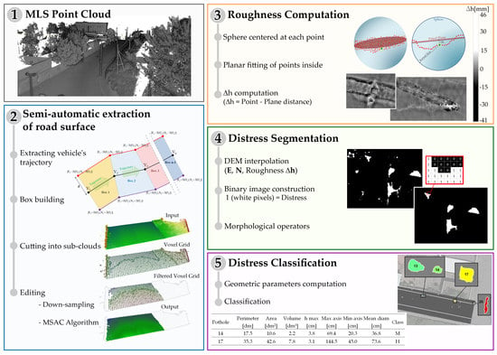
1. Introduction
The civil infrastructure pavement has a life cycle in many stages including design, construction (which includes new construction as well as preservation, maintenance, and rehabilitation), use and end-of-life. Since all pavements deteriorate over time, according to the Life Cycle Assessment (LCA) their monitoring is essential for road maintenance [1,2].
The reliable monitoring of the state of health of a road is an essential aspect of the infrastructure system, aimed at ensuring the safety and comfort of all users. The use of the most innovative systems of mapping and monitoring of road conditions allows an adequate allocation of resources. The most recent systems are composed of one or more acquisition devices and post-processing applications for semiautomatic or automated data extraction procedures, based on computer vision and image processing algorithms [3].
In the technical literature several definitions of regularity can be found: the Technical Committee of the Permanent International Association of Road Congresses (PIARC), for example, in a report on surface characteristics published as a result of the Word Road Congress held in Brussels in 1987 [4] proposed a classification of surface geometrical characteristics of pavement according to geometric resolution (horizontal and vertical) within certain wavelength classes. Other organizations provide their own definitions: the International Organization for Standardization (ISO) in the ISO-13473 standards defines the surface roughness as the deviations of a surface from a true planar surface [5]. Still different is the definition of regularity given by the American Society for Testing and Materials (ASTM E 867), which associates it with the effects it has on vehicle dynamics [6].
A number of dynamic or geometric indexes are used to evaluate roughness. The dynamic indices are based on a model that simulates the dynamic response of a standard vehicle moving at a constant speed along a road profile; the most widely used is the International Roughness Index (IRI), developed by the World Bank in the 1980s [7]. Geometric indices measure the standard deviation of the deviations of a profile (longitudinal or transverse) of the road surface from a straight line [8].
The distress of the road surface can be of a functional or structural type. Distress is classified as functional if the superstructure is still efficient but has critical issues in terms of regularity and adherence, which can make the drive uncomfortable and unsafe, producing significant damage in the long term.
Distress is classified as structural if the pavement is broken due to cyclical loads, i.e., due to aging, or due to poor design or maintenance. This type of distress includes the so-called localized distress, which significantly reduces the safety of users [9].
The detection of pavement distress, which until now had been based mainly on manual inspections [10,11], has recently been based on the analysis of digital images [12,13,14,15] or on point clouds from LiDAR (Light Detection and Ranging) surveys; this is mainly because the data acquired with manual techniques were often incomplete, risky to acquire and insufficient for the assessment of road conditions [16,17,18].
One of the strong points of LiDAR data is that they are much denser than those measured with manual techniques and also more accurate [19]. Furthermore, the LiDAR survey is fast and does not interfere with traffic flow, thus increasing safety, productivity and efficiency [20,21,22]. This has led many institutions and researchers to study and define guidelines for a correct measurement aimed at using the data acquired with this technique for infrastructure maintenance [23].
Alhsan et al. [24] compute the roughness of road pavements on surfaces reconstructed from terrestrial laser scanner (TLS) data using dynamic indices. Chin [22] focuses on filtering TLS data to make them comparable with IRI dynamic index values determined by standard methods, such as profile measuring instruments including level and rod, inclinometers and inertial profilometers. TLS has also been used for the computation and verification of the faulting of rigid concrete slabs in airport pavements [25] and for the analysis of the flexible geometry of the pavement [26].
If the laser scanner is integrated with other sensors in a ground-based mobile laser scanning system (MLS), high-density, directly georeferenced three-dimensional point clouds can be obtained very quickly [23,27,28]. The assessment of the condition of the pavement made on MLS data is one of the main objectives of researchers and road managing institutions, given the speed of acquisition and the efficiency of the technique [29].
Since the MLS is a multi-sensor system and each sensor is characterized by an error that contributes to the overall accuracy of the survey [30,31], it is also important to analyze them individually in order to estimate the accuracy of the overall data [32]. Barber et al. were among the pioneers in estimating the accuracy and precision of the MLS data in order to validate them from a geometric point of view [31]. The authors assessed the overall accuracy of the LiDAR surveys using GNSS-measured checkpoints, the accuracy was in the order of centimeters.
Their evaluation dates back to 2008. Since then, the performance of laser sensors has greatly improved over the years, it is now possible to acquire point clouds from MLS with higher accuracy, mainly related to the distance from the object and partly to the angle of incidence. Fryskowska and Wróblewski [33] prove that data from MLS can be used for geodetic applications. Their tests demonstrate the possibility of measuring the height of the scanned points with an accuracy of a few millimeters, up to distances of the order of 5 m from the laser, i.e., in the range of distances involved in surveying the road surface.
There are many studies on the use of MLS for road surveys [28,34], focused on the identification of the paved surface and roadsides [35,36,37,38], the extraction of road markings [16,39,40,41] and other artifacts such as light poles [42].
Most of the methods developed to detect road surface defects from LiDAR data are based on the construction of a best-fitting plane and the computation of the residuals of the plane fitting. Kumar et al. [43] have studied an automated method for the detection of road roughness using MLS, computing the residual values with respect to a planar reference surface. Later, Kumar et al. [44] proposed a different methodology for the automatic identification of localized surface defects using morphological operators, multi Otsu threshold [45] and 3D binary morphological filters applied to a grey-scale intensity surface.
Díaz-Vilariño et al. [46] proposed a method based on the evaluation of roughness indicators from MLS data to automatically segment and classifies road pavements (asphalt or stone), using K-means algorithms. The authors analyze different roughness indicators, in particular, the arithmetic mean of the absolute values and the root mean square of the residual values appear as reliable roughness indicators that allow a correct classification. Van der Horst et al. [47] have also used K-means clustering to obtain an objective and detailed classification of damage (craquel, rafeling, longitudinal and transverse cracks, potholes). Finally, mathematical morphological operators have been used to filter data.
The identification of surface defects requires processing preceded by a preliminary step of filtering the raw data. In the literature, different methods of filtering and extracting the road surface have been proposed, which can be classified into two main categories: processes based on the direct extraction of the paved surface and processes based on the detection of roadsides [38]. One of the first studies on the extraction of particular elements present on the scene was conducted by Manandahar et al. [48] using segmentation algorithms on scanning lines to distinguish and extract vehicles, trees and walls from the road surface.
Most of the approaches and methodologies proposed in the literature to identify the edges of the road surface have been developed for some situations, such as the presence of great variations in height between contiguous elements at the border areas (e.g., the presence of a curb or sidewalk). The presence of removable objects that do not belong to the road surface could be a major limitation to the success rate of these methods. Among the best-known studies is McElhinney et al. [49] which propose a process divided into two main steps: in the first step, cross-sections are extracted, in the second step, sections are analyzed according to slope values, returned intensity, returned pulse width, and proximity to the vehicle to determine the road edges.
Ibrahim and Lichti [50] describe a method in five steps to detect the curb: organizing the 3D point cloud and nearest neighbor search, 3D density-based segmentation to segment the ground, morphological analysis to refine out the ground segment derivative of Gaussian filtering to detect the curb. Topology and smoothness of road and the local shape features of point clouds are used by Yang et al. [51].
Kumar et al. [37] develop a method of roadside extraction based on the generation of a 2D raster by combining elevation, reflectance and amplitude values of the reflected wave. Guan et al. [40] develop a curb-based extraction method, in which point cloud cross-sections, orthogonal to the MLS trajectory, are extracted from the point cloud, then pseudo-scan-lines are created to detect small height jumps caused by road curbs. Balado et al. [52] introduced a method based on the use of a combination of geometrical and topological characteristics to classify some elements of street furniture (roads, sidewalks, treads, risers and curbs).
There are few extraction methods designed in situations where the edges of the road surface are not easily identifiable, mainly in rural and suburban areas. Among them, Yoon and Crane [53] identified the paved surface by computing the slopes and standard deviations of the elevation values of the single extracted profiles. Smadja et al. [35] use a second-degree polynomial regression to interpolate the points of a generic cross-section; Interpolation is made by applying the Random Sample Consensus (RANSAC) algorithm, which estimates the parameters of the mathematical model by iterative processes.
Recently, Yadav et al. [38] have proposed a method, designed for complex areas, divided into three steps: in the first step the elements and objects that are on the road surface and that do not belong to it are removed, thus dividing the ground points from the no-ground points; in the second step the topology and spatial density are analyzed, together with the intensity values to extract the paved surface; finally, in the last step the contours of the identified surface are analyzed and refined in order to obtain polylines of the pavement edges.
The aim of our work is to develop a procedure for processing the data acquired by MLS, starting from the filtering phase to extract only the points belonging to the ground up to the identification and quantification of some of the main localized degrades that most affect safety, namely swells, shoves and potholes.
2. Test Case and Data
The area to be surveyed is located in an urban environment in the municipality of Rome (Italy). The test was carried out on a stretch of road (Figure 1). The road extends for about 100 m; it proceeds in a straight line for 80 m, then curves. The cross-section is typical of a two-lane road with a single carriageway 11 m wide; each lane is 3.50 m wide. Both sides of the road are used as parking.
The MLS data were acquired by a mobile laser scanner mounted on the roof of a vehicle driving on the road. The measuring head is equipped with two Riegl VQ-450 laser scanners, symmetrically configured on the left and right sides, pointing to the rear of the vehicle with an inclination angle of approximately 145°, as well as inertial and GNSS measurement equipment, housed under an aerodynamically-shaped protective cover. This configuration is called ‘Butterfly’ or ‘X’ pattern. Each VQ-450 scanner generates its own 360° ‘full circle’ profile by the motorized scanning mechanism of the mirrors. The laser’s acquisition frequency is 550 kHz. The main characteristics of the MLS used are listed in Table 1.
A complete road survey was carried out at a driving speed of about 10 km/h. The output data are point clouds directly georeferenced in the UTM/ETRS00 cartographic system [54].
The density of the points of the MLS cloud depends both on the instrument-target center distance and on the angle of incidence. For an average distance of 5 m, at a vehicle speed of 10 km/h, the value of the point-density is estimated at 32,544 points/m2, while it decreases to 4688 for a speed of 60 km/h. Figure 2 shows the actual density maps (not estimated). The distance between the scanning lines is approximately 1.2 cm and 7.0 cm, respectively for driving speeds of 10 and 60 km/h.
Follow-up analyses were made on the densest cloud, the one acquired in only one travel direction, at a driving speed of 10 km/h.
3. Methods
The proposed method aims both at identifying the relevant distresses and at estimating their size. Data processing has been carried out in four main steps (Figure 3 shows a workflow of the procedure):
- the first step focuses on editing the MLS point cloud to extract only the points belonging to the road surface;
- the second step consists in evaluating the roughness, determining the height deviation of every single point of the cloud with respect to the reconstructed model of the pavement surface;
- the third step involves the creation of a binary image starting from the built DEM; two different images will be created and analyzed separately, one for positive displacements, the other for negative ones;
- the last step, the fourth, focuses on the computation of the main geometric parameters of each segmented region. According to these, each region will be classified according to the severity levels given in the standards.
3.1. Semi-Automatic Extraction of the Road Surface
The first step of the whole process that will lead to the identification and classification of the distress is the editing of the point cloud to remove the outliers and extract the bare road surface, as shown in the workflow of Figure 3. This phase consists of four steps:
1. Extracting the vehicle’s trajectory from the LAS data
To extract from the whole cloud of laser points only a few points that will be the vertexes of the polyline representative of the vehicle’s trajectory, the points acquired with a given scanning angle are extracted. The matrix containing the planimetric coordinates of the points acquired with a scanning angle equal to 0° has been ordered, in ascending order, according to GPS time (value measured for each single point). The first vertex V1 of the polyline is identified by the planimetric coordinates contained in the first line of the matrix thus ordered. Starting from the first vertex V1 all points contained in a sphere with center at the point itself and radius equal to the length of the polyline segments are extracted. The function used is the ‘findNeighborsInRadius’. In our test case, the polyline segments are 5 m long. The function outputs the line indices of the matrix containing the planimetric coordinates of the points inside the sphere and the distances of each point from its center. The next vertex V2 of the polyline is identified by the planimetric coordinates of the point having the greatest distance from V1 and the largest GPS time. V2 is the center of the next research sphere. The cycle repeats until the coordinates of all polyline vertices are found. Figure 4 shows a schematic drawing of the procedure for constructing the polyline that discretizes the vehicle’s trajectory.
Extracting sub-clouds inside built-up boxes
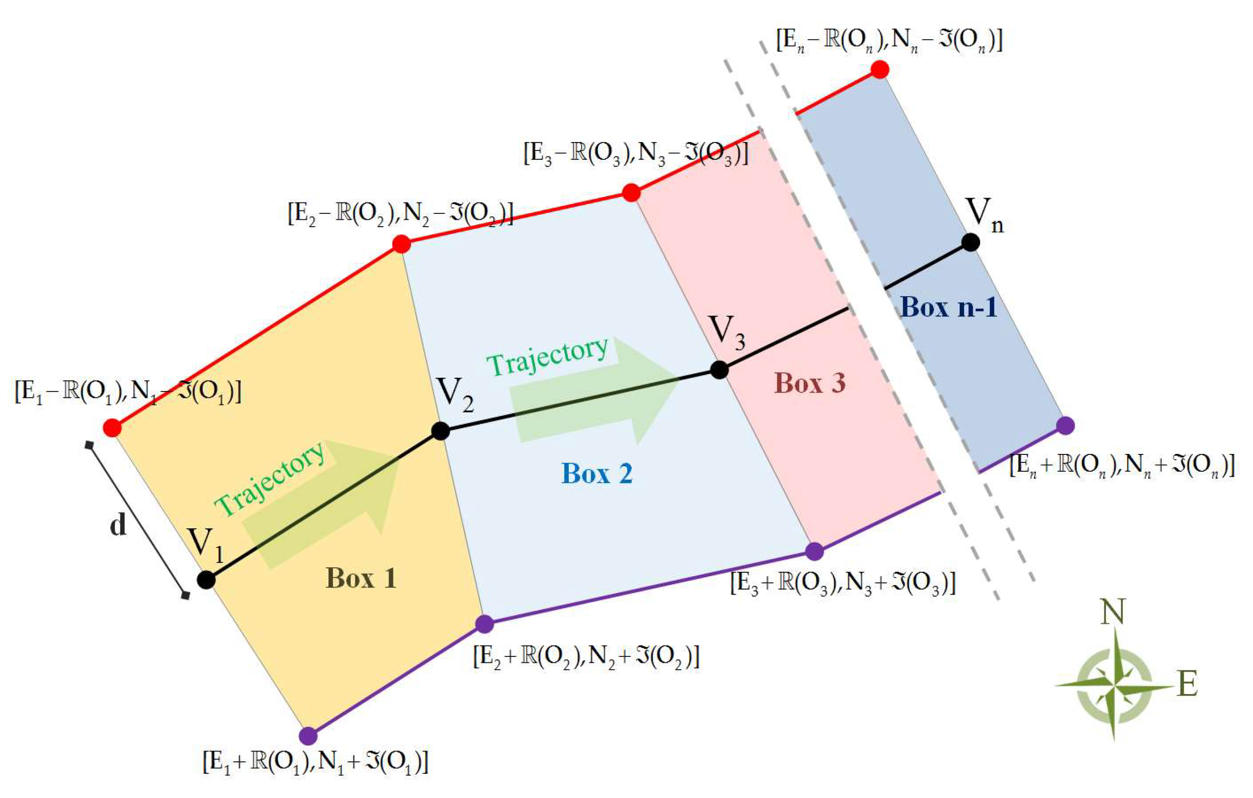
2. To reduce the CPU time, the whole point cloud has been divided into many sub-clouds, whose points are contained in polygonal boxes purposely built to divide it. The vertices of the boxes are aligned in a direction orthogonal to the polyline that describes the trajectory of the vehicle.
Given the n vertices V of the polyline, whose coordinates are contained in the matrix , to compute the coordinates of the offset points, a row vector is built, which contains the coordinates Ev, Nv (East and North respectively) of each vertex v of the polyline:
where im is the imaginary unit, i.e., im = 0.0000 + 1.0000·i.
Then, the row vector , which contains the coordinate differences between the vth vertex and the vth−1, is built:
Then it is built the row vector :
where ΔM1 indicates the first element of ΔM, ΔM1:n−2 indicates the elements of ΔM from the 1st to the nth−2 (with n = number of vertices) and ΔMn−1 indicates the last element of the row vector ΔM, which has the dimensions (n − 1).
For each pair of planimetric coordinates Ev, Nv of the generic vertex v the two pairs of offset coordinates are obtained by subtracting and adding the scalar of the real or imaginary part of the respective row of the matrix .
Once a certain offset value d is set, the coordinates of the vertices of the box are:
where:
The ‘offset points’ correspond to the vertices of the quadrilateral (the boxes). The length of the boxes is that of the segments of the polyline, the width varies depending on the width of the carriageway. In our case, the dimensions of the boxes are 10 × 5 m. Figure 5 shows a scheme of the construction of the boxes.
3. Down-sampling of the point cloud
The next step consists of down-sampling the point cloud to obtain the nodes that are used as the center of the research spheres for the follow-up road surface extraction process. To do this, the Matlab function ‘pcdownsample’, method ‘gridAverage’, has been used. A regular voxel grid is built with a user assigned step. The height values of the points surrounding the grid node are averaged and the average is assigned as the height value to the node. Before proceeding with the editing process, nodes in areas outside the road surface must be removed. By using the ‘pcnormals’ function, for each node in the down-sampled grid, a plane has been fitted by least squares and the normal vector to it has been estimated. Points whose normal vector has a component along the z axis (with z in the direction of the ellipsoidal height) of less than 1 (with a margin of error of 5 × 10⁻³) have been removed. Finally, the ‘pcdenoise’ function has been applied to remove isolated or edge nodes.
4. Road surface extraction
In the last editing step, we used the M-estimator SAmple Consensus (MSAC) algorithm, which is a robust variant of the Random Sample Consensus (RANSAC) algorithm, an iterative method to estimate the parameters of a mathematical model from a set of observed data that contains outliers [55].
The processing steps are:
- Starting from the remaining nodes of the voxel grid, using the ‘findNeighborsInRadius’ function, a sphere centered in each node is built. The radius of the sphere has been chosen to be proportional to the grid step; it is recommended to choose a radius value such that two adjacent spheres have a large overlapping area, for example, three times the grid step.
- Using the ‘pcfitplane’ function, the points (of the original point cloud) falling within the sphere are fitted on a plane, the parameters of whose equation are estimated. The variables of the function are: the ’maxDistance’ between the plane and the generic point so that it can be considered an inlier, the ‘referenceVector’ which is a constraint on the orientation of the reference plane, and the ‘maxAngularDistance’, which is a threshold value for the angular distance between the normal vector of the fitted plane and another vector (in the direction of the ellipsoidal height). Since the plane has been created with the iterative MSAC process, its position cannot be fixed a priori, the plane must be able to rotate in space: this is why it is required to set a threshold value for the ‘maxAngularDistance’. Moreover, since in our case we want to identify surfaces with mostly “horizontal” position, a ‘referenceVector’ dim [0,0,1] has been used.
- Once the outliers have been removed, the cycle starts again on one other grid node until the editing process is complete.
3.2. Roughness Evaluation
The evaluation of localized distress in 3D space is rather complex; there is no ideal reference surface to model so that any anomalies present can be measured with respect to it. It could be considered to use a plane to characterize a single lane and determine the height variations of the road surface with respect to this one [43]. Nevertheless, there are essentially two main problems in this approach: it is not trivial to choose the longitudinal dimensions that the reference plane should assume; the sides of a plane must coincide with the sides of adjacent planes; this is a very rigid constraint.
That is why we have decided to use several local reference planes, built gradually for each point of the cloud belonging to the road surface. The procedure follows the following steps:
- A sphere with an assigned radius (kernel size) and center at each point of the cloud has been built (Figure 6).
- All the points inside the sphere are fitted on a plane. The ‘findNeighborsInRadius’ function has been used to select the points. The plane has been fitted to data with a least-squares robust regression, the ‘Bisquare Weights’. This method minimizes a weighted sum of squares, where the weight of each data point depends on its distance from the fitted plane; the farther away is the point, the less weight it gets.
- Finally, the roughness value Δh is computed as the distance between the point (center of the sphere) and the fitting plane. Positive values of Δh indicate that the point is below the plane (downward deformations) while negative values are defining the upward deformations.
Besides the computation of Δh, the algorithm provides in output, as an estimation of the goodness of the fitting, the RMSE (Root Mean Square Error) value, that is also associated to all the point of the cloud; its layout contributes to give a judgment of the road surface conditions.
3.3. Distress Identification and Evaluation
The quantification and classification of the different distress of the road surface has been done using image segmentation algorithms, treating the point cloud as a digital image in which pixels are grouped according to specific conditions. The implemented procedure follows the following steps:
1. Interpolation of the roughness values Δh on the nodes of a grid
The coordinates of the point cloud (N, E, Δh) have been interpolated to build a raster DEM where the coordinate h is replaced with the roughness value Δh. For the building of the DEM the IDW (Inverse Distance Weighted) interpolator (with distance power 2) implemented in Surfer® ver. 12 by Golden Software was used [56]. We chose it because, although it is a very common deterministic interpolator, it works well for high-density LiDAR data [57]; moreover, in [58] some comparisons made with reference DEM have shown a better correlation when using IDW than using other more robust interpolation methods.
The spatial resolution ρ of the DEM was chosen according to two parameters that characterize any scan: the minimum surface density value and the mean shortest distance between the scan lines. The mathematical formula that gives the resolution as a function of surface density, for a quite regular distribution of points such as the test-case is [59]:
where A is the surface area of the scanned site and N is the total number of points in the area A. The simplified formula that gives the grid density as a function of the average distance between adjacent scan lines is [59]:
where di,j is the average distance between scan lines. The resolution of the DEM must be equal to or greater than the maximum value between those computed in this way. In our test case the (6) gives 0.8 cm in output and the (7) one gives 1.1 cm. The resolution of the DEM we have chosen is 1.5 cm.
2. Creating a binary image
The raster DEM, in which the pixel size corresponds to the grid step, has been transformed into a binary image. To the pixels with Δh greater in absolute value of a given threshold value (different for upward and downward displacements) is assigned the value 1 (that corresponds to white) while to all the other pixels is assigned the value 0 (black pixels). The white pixels will, therefore, be those affected by distress while the black pixels will be those not affected. Two separate binary images are created for positive and negative roughness values. Figure 7a shows an example of a section of road affected by downward displacements.
3. Computation of geometric parameters and segmentation
The next step is the implementation of both geometric and morphological operators in order to remove or group isolated white pixel regions with certain characteristics; this is the proper segmentation. The main geometric parameters computed for each region of the binary matrix are: perimeter, area, volume (Figure 8).
Given the coordinates (xp,k,yp,k) of the vertices of the n segments of the polyline that makes the outline of the distress, the perimeter is computed as:
The area has been computed as the sum of the pixels of each region. The volume has been computed as:
where Δij is the pixel size, Δhj is the height of each pixel and npx is the total number of pixels in each region.
In this step, other geometrical parameters were also computed, such as the length of the axes of the circumscribed ellipse (‘regionprops’ function) to be used together with the previous ones for the identification of the zones to be segmented. Their selection is based on the values assigned to the parameters set in accordance with the specifications provided by ASTM-D6433 [11].
In particular, the following parameters have been analyzed for the segmentation:
- Δh values. The regions will be divided according to the level of severity, which in turn depends on the depths or heights of the distress.
- Area. The level of severity of distress is a function not only of its dimension in elevation but also of its extension in planimetry.
- Length of the axes of the circumscribed ellipse and the mean diameter (‘regionprops’ function). In addition to the extent that distress may have, the other parameters that affect the severity levels are the mean diameter and orientation with respect to the direction of travel.
The geometrical parameters mentioned above have been combined and analyzed according to the type of distress (downward or upward displacements) that is to be characterized. The removal of regions that do not meet the requirements is based on a cycle of conditional instructions, implemented using the ‘RemoveMask’ function.
Finally, expansion and erosion operators have been applied on the binary image to add or remove pixels on the boundaries of the regions in order to obtain a regular contour of the distress. Contours of the regions have been identified using the ‘bwboundaries’ function, based on the ‘Moore-Neighbor’ tracking algorithm, modified by Jacob’s stopping criterion [60] and the morphological functions ‘strel’ and ‘imfill’ have been implemented [61,62]. Figure 7b shows an example of the output.
4. Results
4.1. Extraction of the Road Surface
This phase aims at removing the outliers and extracting only the surface of the road pavement. For computational constraints, the whole point cloud has been divided into 25 polygonal boxes each with a size of 12 × 5 m, built around the trajectory of the vehicle reconstructed by extracting from the MLS point cloud the only points with a scanning angle of 0 degree (with a margin of error of 5 × 10⁻³). These points were interpolated linearly to construct a polyline made of 5 m long sections. Only 20 boxes, (from 5th to 24th) were considered for the next editing step.
Figure 9 shows the 25 polygonal boxes built to divide the cloud into sub-clouds (a); in (b) a zoomed excerpt of the points of the cloud corresponding to the MLS track is shown.
On the points belonging to each box, a voxel grid (step size 0.20 m) has been built in order to down-sample the original point cloud. On the nodes of the voxel grid the RANSAC-based plane fitting algorithm was run, and a sphere with a diameter 3 times the grid step, namely 0.60 m, has been built to remove the outliers.
The following were considered as outliers:
- the points that have a distance from the plane greater than the selected threshold. In our test we set a threshold absolute value of 2.5 cm, within the range of values corresponding to the pavement’s macro-texture;
- points belonging to a plane whose normal has a z component that differs angularly more than the selected threshold from the direction of the ellipsoidal height. To choose the input value for this parameter, namely ‘maxAngularDistance’, we made a few tests. Given unchanged values for the other parameters, most damaged areas were removed for angles less than 5°. For angles greater than 10°, some points not belonging to the road surface were not removed, in detail along the edges and in correspondence of objects present on the road surface. In our test case, the value that led to better results was 10°.
4.2. Roughness Evaluation
The test was carried out on an area characterized by a variety of degradation, at different levels of severity, chosen to test and validate the proposed method. In this phase was computed, as described in Section 3.2, the difference in height of each single point belonging to the point cloud with respect to the reference plane, constructed by interpolating on it the points belonging to a sphere of a given radius. The only parameter to set is, therefore, the radius of the sphere (the size of the kernel). The kernel size has been set to 0.60 m, congruent with some distress evaluation.
The result is a point cloud where each point is associated with a scalar representing the distance between the point and the corresponding plane. Positive values indicate downward displacements (potholes) while negative values indicate upward displacements (swells/shoves).
Figure 12 shows the roughness value Δh computed for each point of the cloud, the grey tone represents its value.
Positive values (towards white) represent the points below the reference plane, while negative values (towards black) represent the points above it. The maximum value found for the potholes was 46 mm, while for the swells/shoves was 41 mm.
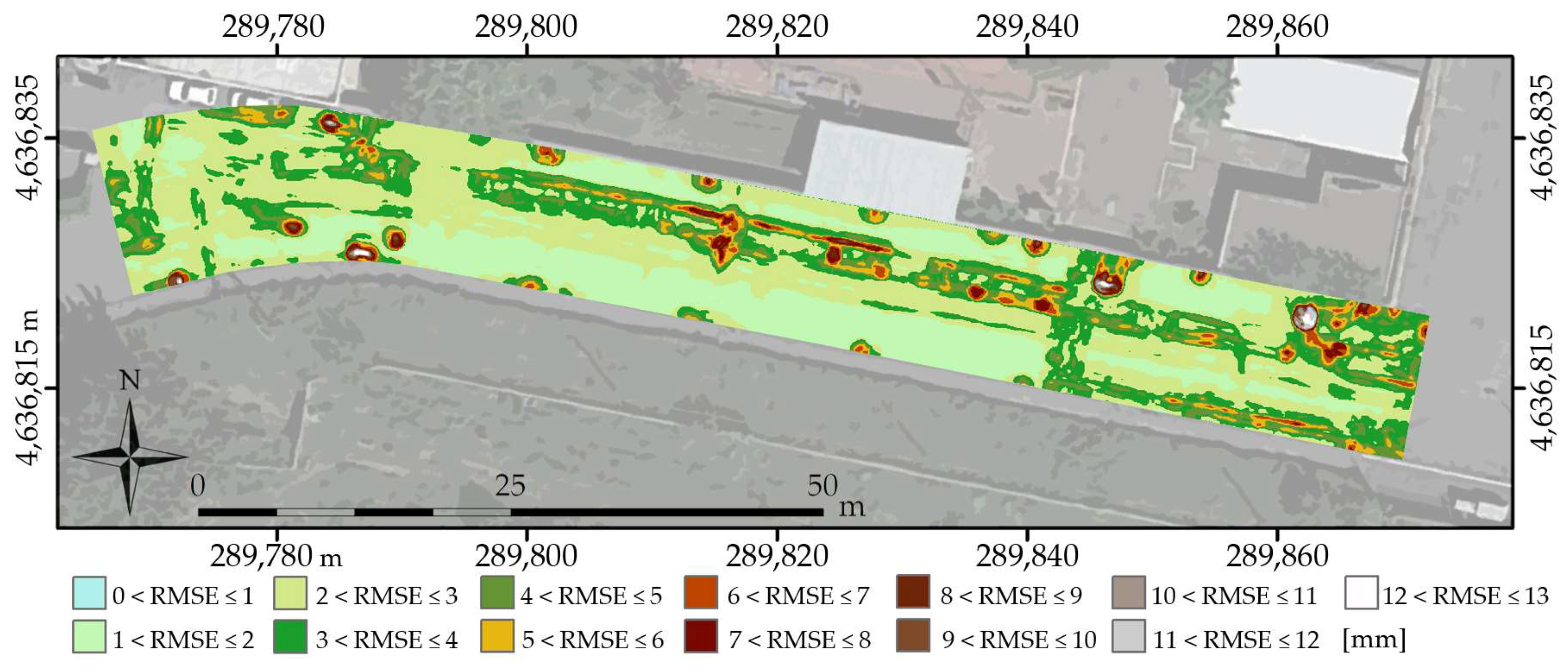
Figure 13 shows the Root Mean Square Error (RMSE) associated with the points in the cloud. It was computed to assess the goodness of fit, it is also significant for an initial classification of the pavement condition. Areas with low RMSE values should correspond to regular paving conditions (good road surface condition), while high values show surface irregularities (poor condition).
4.3. Distress Identification
The point cloud with the roughness values put in place of the heights was interpolated on a DEM grid using the software package Surfer® ver. 12 by Golden software [56]. The inverse distance interpolation method (power 2) of the grid was used. The grid step was set to 1.5 cm, depending on the density of the MLS data. The search radius was set to 0.50 m. The output grid is a matrix, in which a roughness value is assigned to each cell.
The next step concerns the segmentation for the extraction and cataloging of surface distress, according to the severity levels introduced by the standard [11]. The estimated distresses have been divided into two main categories:
- downward displacements, that includes depressions, cracking, potholes, rutting, etc.
- upward displacements, that includes slides, bumps, swells, shoves, patches, etc.
Among the downward displacements we have focused our analysis on the potholes, which are small, usually less than 750 mm in diameter, bowl-shaped holes in the pavement surface. To decide the parameters to be set for segmentation, we have assumed that they are not to be defined as such if they have a diameter less than 100 mm and severity levels are significant when the depth exceeds 13 mm. In addition, standards and literature define them as dangerous when they are more than 1 inch (about 25 mm) deep and the area is greater than 1 square foot (about 1 dm2, which corresponds to an average diameter of about 55 cm) [63].
Consequently, only regions with axes smaller than 100 mm, area smaller than 1 dm2 and roughness values Δh, positive, smaller than 13 mm have been discarded.
Among the upward displacements, we have focused our analysis on swells and shoves. Swell is characterized by un upward bulge in the pavement’s surface whereas shove is a permanent, longitudinal displacement/ripple of a localized area of the pavement surface. Swelling looks like as a long, gradual waves more than 3 m long and shows as short, abrupt waves on the pavement surface. Both can make the ride uncomfortable and unsafe, producing significant damage in the long term. These types of distress tend to be mostly functional, i.e., the superstructure is still efficient but has some critical issues in terms of regularity and adherence.
As far as swells/shoves are concerned, only regions with an area smaller than 10 dm2 and |Δh| larger than 5 mm (Δh negative) were discarded. Figure 14 shows the identified distresses, which are 29 potholes and 98 swells/shoves.
In the test case, the clearly recognizable swells are the number 25, 35, 38, 45, 49, 66 and 72 (Figure 14b) mainly oriented along the direction of travel and longer than 3 m. The shoves are all isolated segmented regions. Most were formed by the longitudinal acceleration (braking, speed up) of the tire and the vehicle load. Some of these, on the other hand, was formed due to poor compaction and the thrust (by the vehicles) of the superficial part of the pavement against the hydraulic devices consisting of more rigid elements (16, 57, 77, in Figure 14b), their shapes clearly outline manholes. The segmented regions are congruent with the particular configuration of the type of distress, i.e., swollen and isolated areas with longitudinal development, as shown in Figure 14b, numbers 10, 24, 22, 19, 60 and 73.
In addition, the distresses have been classified according to the severity levels deduced from ASTM D6433 [11], Table 2. The severity levels are divided into low (L), medium (M) and high (H). By adopting a speed of travel suited to the type of road being examined, a low level of severity corresponds to a situation where a reduction in speed is not necessary to respect good levels of comfort and safety, even with the presence of different types of distress.
Localized distresses can create vibrations and jerks of the vehicle that only cause minor discomforts to the driver. A medium level is synonymous with significant vehicle vibration; speed reduction is necessary to ensure good levels of safety and comfort. A high level of severity highlights a situation where vibrations and jerks are so strong that the user is forced to significantly reduce the transit speed in order to achieve an acceptable level of comfort and safety; localized distresses create significant discomfort, as well as a high risk of damage to the vehicle.
In the test case, the most concerned are 21 potholes, in particular, 16 with a medium severity level and five with a high severity level. As far as swells/shoves are concerned, most (93) were found to be of low severity level and only five of medium severity level. During maintenance, in addition to the category of road that also determines the degree of priority, the geometric characteristics of the distress provide the parameters used to estimate the intervention time limit. The maximum time allowed between identification and repair depends on two factors: the size of the pothole and the hierarchy of the road. Both factors have an impact on the hazard and the level of risk created by the pothole itself. Potholes with a high level of severity, for main roads (e.g., motorways) should be repaired within 5 h after identification [63]. At the same time, potholes with a ‘medium’ level acquire different weights as the level of the hierarchy of the road changes.
For all identified distresses the main geometric parameters have been computed, i.e., for the potholes the perimeter, area, volume, maximum depth, axes of the circumscribed ellipse and the mean diameter, while for the swells/shoves only the perimeter, area, volume and maximum depth.
Table 3 shows, for some significant examples of identified distresses (both potholes and swells/shoves), the computed geometric parameters.
5. Discussion
The results obtained with the proposed method depend mainly on the value of the parameters given as input to the software. In particular, in the editing phase, it is important to choose the correct values because the reconstructed 3D model of the road surface represents the reference surface on which the distresses will be highlighted.
The choice of some parameters is based on considerations related to the nature of the input data: the DEM resolution, for example, is in relation to the characteristics of the point cloud, i.e., its density and accuracy. Other parameters are decided according to the type of distress to be identified. For others, some tests have been carried out to verify the influence of the choice of certain values on the results. In the segmentation procedure (see Section 3.3), the parameter that most affects the results is the search radius for fitting points on a local plane, i.e., the size of the kernel.
To study the effect of this parameter on the results, we segmented the image and evaluated the distresses highlighted when the kernel size changes from 0.1 to 1 m, in 10 cm steps. The stretch of road analyzed is 5 m long (transparent white rectangle in Figure 15). In that stretch there is a pothole (the number 14 visible in Figure 14a) and some shoves and swells (number 44, 45, 46, 47 and 49 in Figure 14b); their geometric parameters are reported in Table 3.
Figure 15 shows the results obtained when the kernel size changed. Segmented areas (i.e., those defined as having significant distress) are outlined in black. The color scale indicates the estimated roughness value Δh (see the legend), which varies between 0 to 2 cm for shoves/swells and 0 to 4 cm for potholes.
Changes in the shape and size of segmented distresses are clearly visible; one can see how distresses tend to appear and increase in size as the kernel size increases. More in details for potholes note that, with a kernel size of 0.10 m, nothing is highlighted because the local plane is too small and follows the trend of the road surface; increasing the kernel size to 0.20 m a region characterized by positive Δh values (i.e., a pothole) appears; this area stabilizes from 0.60 m onwards, when its size is completely within the kernel size. For shoves/swells, note that, by increasing the kernel size, they gradually appear as they do for potholes but never stabilize.
The results of these tests confirm for us that the choice of value for this parameter is not trivial, hence it is tricky to recommend a criteria of unambiguous choice. A more reliable assessment could be made by analyzing the variation in the severity level of the distress as the kernel size changes, regardless of the variation in the geometric parameters. For this analysis, we have selected some distresses, chosen because they are isolated and well distinguishable, i.e., not characterized by overlapping of different degrades.
Figure 16 shows how the level of severity attributed to the analyzed distresses may vary with the size of the kernel. It can be seen that some distress do not change class as the kernel size changes, while others vary more classes as it changes. These last cases concern, in particular, several distresses with positive Δh value that, more than real potholes, are pitting that smoothly degrade.
Note also that all swells/shoves analyzed, from a kernel size of 0.60 m onwards, maintain the same level of severity while the potholes vary in severity level, but also tend to stabilize from 0.60 m onwards.
Figure 17 graphically shows the values of the most relevant geometric parameters of the distresses listed in Figure 16, as the kernel size changes. In particular, as for the h max value, graphs show that, in most cases, there is a variation in the slope of the lines interpolating the values of h max near the kernel size value of 60 cm. To run the linear interpolation, the ‘ransac’ function, implemented in Matlab, has been used; the algorithm works, also here, using the MSAC method.
For this reason, in our test area, where the road profile is very irregular, we have chosen a kernel size of 0.60 m. Yet, we want to underline once again the non-triviality of the choice of this parameter.
Another critical aspect about the Δh computation procedure, is the so-called ‘boundary effect’, In the roadside areas, for an extension equal to the size of the kernel, the research sphere falls in part out of the roadway, thus the number of points that will be fitted on a plane decrease as you approach the edge of the road (to become about half).
As a result, the Δh values associated with the points belonging to the boundaries are less reliable than the others. To check this aspect, a simulation was made by computing the Δh for the points of a central portion of the roadway of about 2 m2, selected in the middle of the roadway. Figure 18a shows an excerpt of the point cloud, the grayscale is proportional to the Δh values computed with a kernel size of 0.60 m. The area framed in white shows the 2 m2 sub-cloud used for the simulation. For that piece, the difference between the Δh values computed considering the whole point cloud of Figure 18 (roughness values not influenced by the boundary effect) and the values computed considering only the sub-cloud (values influenced by the boundary effect) has been computed.
Figure 18b shows the differences δh between the two values, classified in 0.5 mm steps (see legend).
As expected, the boundary effect exists, the δh in absolute value reaches 3 mm. Hence, the roughness values computed on the boundary strips (outside the area framed in black) are unreliable and there could be a mistake in the attribution of the severity class of the distresses in these zones. It is therefore suggested to exclude from the analysis the whole boundary strip having the width equal to the kernel size.
6. Conclusions
In this note, we wanted to highlight the potential of using the LiDAR survey technique, one of the most interesting and continuously developing remote sensing techniques, in order to assess the ‘state of degradation’ of the road pavement. The technique has proved to be effective in providing data that allow usto build a 3D model of the infrastructure surface.
As the applications of this technique to infrastructure surveying are recent, there are still many critical aspects to evaluate. Commercial software available implement only a few functions, in response to the specific needs of professionals and, therefore, do not fully satisfy the scientific community. In an attempt to overcome these limitations, the problems that arise in the application of the technique to road survey have been analyzed and the studied algorithms have been implemented in proprietary software (in Matlab® environment) and tested on a case study.
The point clouds acquired are not directly usable, but they must first be filtered to remove outliers (vegetation, cars, pedestrians, etc.) and extract only the points belonging to the roadway in a semi-automatic way. The implemented algorithm is based on the MSAC method, a robust estimate of the parameters of a mathematical model from a data set containing outliers.
The evaluation of localized distresses in 3D space is rather complex; there is no exact reference surface to estimate any anomalies present with respect to it. In order to quantify and analyze the different types of distress, in particular, the regularity that affects the comfort of users and some localized distresses, mainly responsible for the safety of the infrastructure, it was decided to use a local reference plan, built around each point belonging to the road surface, with respect to which to compute the roughness of each point of the cloud.
The results obtained with the proposed methodology partly depend on the choice of the parameters provided as input to the computation software. The choice of some of them is based on considerations related to the nature of the input data. The resolution of the DEM, for example, is mainly related to the characteristics of the point cloud (density and accuracy) whereas the values to be given to other parameters are suggested by the type of distress to be segmented.
In particular, the choice of kernel size has significant consequences and strongly affects the segmentation process. The sensitivity with which the geometric parameters of the identified regions vary, as the kernel size varies, does not allow an easy and justified choice of the latter. A better evaluation can be made evaluating the variations in the severity levels in place of analyzing the variations in the geometric parameters.
With regard to the procedures implemented, the experimental results have shown that the choice of parameters to be entered by the user for the extraction of the roadway or distress analyzed is not trivial as it strongly influences the results. Due to the complexity of the configuration of the different distresses and the geometry of the roadway, it is appropriate to choose these parameters according to the boundary conditions, it is not possible to identify and set default values valid for any condition.
The segmentation procedure implemented has however allowed us to extract some types of distress in an effective way; the parameters used in the test case have made it possible to correctly segmented and identify the types of distress analyzed, also congruent with some in-situ inspections.
Author Contributions
All authors contributed to the conception and design of the work. In more detail, M.F. and A.D.B. focused on methodological, algorithmic and practical aspects of the numerical processing of the surveyed data, M.R.D.B. has focused on the interpretation of the results as regards the characterization of the road surface. All authors wrote the draft of the paper. All authors have read and agreed to the published version of the manuscript.
Funding
The research is supported by the Italian Ministry of Education, University and Research under the National Project “Extended resilience analysis of transport networks (EXTRA TN): Towards a simultaneously space, aerial and ground sensed infrastructure for risks prevention”, PRIN 2017, Prot. 20179BP4SM.
Acknowledgments
The authors would like to thank SINA S.p.A. (Società Iniziative Nazionali Autostradali) for the collaboration in data acquisition.
Conflicts of Interest
The authors declare no conflict of interest.
References
- Santero, N.J.; Masanet, E.; Horvath, A. Life-cycle assessment of pavements. Part I: Critical review. Resour. Conserv. Recycl. 2011, 55, 801–809. [Google Scholar] [CrossRef]
- Harvey, J.; Meijer, J.; Kendall, A. Life Cycle Assessment of Pavements: [Techbrief]; Federal Highway Administration: Washington, DC, USA, 2014. [Google Scholar]
- Ragnoli, A.; De Blasiis, M.R.; Di Benedetto, A. Pavement distress detection methods: A review. Infrastructures 2018, 3, 58. [Google Scholar] [CrossRef] [Green Version]
- PIARC. Technical Committee Report on Surface Characteristics. In Proceedings of the Surface characteristics report n.1 - Piarc XVIII World Road Congress, Brusels, Belgium, 13–19 September 1987; PIARC: Paris, France, 1987. [Google Scholar]
- ISO. Characterization of Pavement Texture by Use of Surface Profiles; ISO-13473; ISO: Geneva, Switzerland, 2002. [Google Scholar]
- ASTM. Standard Terminology Relating to Vehicle-Pavement Systems; E867-06; ASTM International: West Conshohocken, PA, USA, 2012. [Google Scholar]
- Gillespie, T.D.P.; William, D.O.; Sayers, M.W. Guidelines for Conducting and Calibrating Road Roughness Measurements; WTP46; The World Bank: Washington, DC, USA, 1986. [Google Scholar]
- Muniz de Farias, M.; de Souza, R.O. Correlations and analyses of longitudinal roughness indices. Road Mater. Pavement Des. 2009, 10, 399–415. [Google Scholar] [CrossRef]
- Bella, F.; D’Amico, F.; Ferranti, L. Analysis of the effects of pavement defects on safety of powered two wheelers. In Proceedings of the 5th International Conference Bituminous Mixtures and Pavements, Thessaloniki, Greece, 1–3 June 2011. [Google Scholar]
- ASTM. Standard Test Method for Measuring Rut-Depth of Pavement Surfaces Using a Straightedge; E1703M-10; ASTM International: West Conshohocken, PA, USA, 2015. [Google Scholar]
- ASTM. Standard Practice for Roads and Parking Lots Pavement Condition Index Surveys; D6433-18; ASTM International: West Conshohocken, PA, USA, 2018. [Google Scholar]
- Shen, G. Road crack detection based on video image processing. In Proceedings of the 2016 3rd International Conference on Systems and Informatics (ICSAI), Shanghai, China, 19–21 November 2016; pp. 912–917. [Google Scholar]
- Salini, R.; Xu, B.; Paplauskas, P. Pavement distress detection with picucha methodology for area-scan cameras and dark images. Civ. Eng. J. 2017, 1, 34–45. [Google Scholar] [CrossRef]
- Staniek, M. Detection of Cracks in Asphalt Pavement during Road Inspection Processes; Series Transport; Silesian University of Technology: Gliwice, Poland, 2017; Volume 96. [Google Scholar]
- Zhao, J.; Wu, H.; Chen, L. Road surface state recognition based on svm optimization and image segmentation processing. J. Adv. Transp. 2017, 2017, 21. [Google Scholar] [CrossRef]
- Kumar, P.; McElhinney, C.P.; Lewis, P.; McCarthy, T. Automated road markings extraction from mobile laser scanning data. Int. J. Appl. Earth Obs. Geoinf. 2014, 32, 125–137. [Google Scholar] [CrossRef] [Green Version]
- De Blasiis, M.; Di Benedetto, A.; Fiani, M.; Garozzo, M. Characterization of Road Surface by Means of Laser Scanner Technologies. In Proceedings of the Pavement and Asset Management: World Conference on Pavement and Asset Management (WCPAM 2017), Baveno, Italy, 12–16 June 2017; CRC Press: Boca Raton, FL, USA, 2019; p. 63. [Google Scholar]
- De Blasiis, M.R.; Di Benedetto, A.; Fiani, M.; Garozzo, M. Assessing the effect of pavement distresses by means of lidar technology. In Proceedings of the ASCE International Conference on Computing in Civil Engineering 2019 American Society of Civil Engineers, Atlanta, GA, USA, 17–19 June 2019. [Google Scholar]
- Křemen, T.; Štroner, M.; Třasák, P. Determination of pavement elevations by the 3d scanning system and its verification. Geoinform. FCE CTU 2014, 12, 55–60. [Google Scholar] [CrossRef] [Green Version]
- Glennie, C. Kinematic terrestrial light-detection and ranging system for scanning. Transp. Res. Rec. 2009, 2105, 135–141. [Google Scholar] [CrossRef]
- Yen, K.S.; Ravani, B.; Lasky, T.A. Lidar for Data Efficiency; Washington State Department of Transportation Office of Research and Library Services: Washington, DC, USA, 2011. [Google Scholar]
- Chin, A. Paving the Way for Terrestrial Laser Scanning Assessment of Road Quality; Oregon State University: Corvallis, OR, USA, 2012. [Google Scholar]
- Olsen, M.J.; Knodler, M.A.; Squellati, A.; Tuss, H.; Williams, K.; Hurwitz, D.; Reedy, M.; Persi, F.; Glennie, C.; Roe, G.V.; et al. Guidelines for the Use of Mobile Lidar in Transportation Applications; Transportation Research Board: Washington, DC, USA, 2013. [Google Scholar]
- Alhasan, A.; White, D.J.; De Brabanter, K. Spatial pavement roughness from stationary laser scanning. Int. J. Pavement Eng. 2017, 18, 83–96. [Google Scholar] [CrossRef]
- Barbarella, M.; D’Amico, F.; De Blasiis, M.; Di Benedetto, A.; Fiani, M. Use of terrestrial laser scanner for rigid airport pavement management. Sensors 2018, 18, 44. [Google Scholar] [CrossRef] [Green Version]
- Barbarella, M.; De Blasiis, M.R.; Fiani, M. Terrestrial laser scanner for the analysis of airport pavement geometry. Int. J. Pavement Eng. 2019, 20, 466–480. [Google Scholar] [CrossRef]
- Gandolfi, S.; Barbarella, M.; Ronci, E.; Burchi, A. Close photogrammetry and laser scanning using a mobile mapping system for the high detailed survey of a high density urban area. Int. Arch. Photogramm. Remote Sens. Spat. Inf. Sci. 2008, 37, 909–914. [Google Scholar]
- Guan, H.; Li, J.; Cao, S.; Yu, Y. Use of mobile lidar in road information inventory: A review. Int. J. Image Data Fusion 2016, 7, 219–242. [Google Scholar] [CrossRef]
- Che, E.; Jung, J.; Olsen, M.J. Object recognition, segmentation, and classification of mobile laser scanning point clouds: A state of the art review. Sensors 2019, 19, 810. [Google Scholar] [CrossRef] [PubMed] [Green Version]
- Glennie, C. Rigorous 3d error analysis of kinematic scanning lidar systems. J. Appl. Geod. 2007, 1, 147. [Google Scholar] [CrossRef]
- Barber, D.; Mills, J.; Smith-Voysey, S. Geometric validation of a ground-based mobile laser scanning system. ISPRS J. Photogramm. Remote Sens. 2008, 63, 128–141. [Google Scholar] [CrossRef]
- Toschi, I.; Rodríguez-Gonzálvez, P.; Remondino, F.; Minto, S.; Orlandini, S.; Fuller, A. Accuracy evaluation of a mobile mapping system with advanced statistical methods. Int. Arch. Photogramm. Remote Sens. Spat. Inf. Sci. 2015, XL-5/W4, 245–253. [Google Scholar] [CrossRef] [Green Version]
- Fryskowska, A.; Wróblewski, P. Mobile laser scanning accuracy assessment for the purpose of base-map updating. Geod. Cartogr. 2018, 67, 35–55. [Google Scholar]
- Ma, L.; Li, Y.; Li, J.; Wang, C.; Wang, R.; Chapman, M. Mobile laser scanned point-clouds for road object detection and extraction: A review. Remote Sens. 2018, 10, 1531. [Google Scholar] [CrossRef] [Green Version]
- Smadja, L.; Ninot, J.; Gavrilovic, T. Road extraction and environment interpretation from lidar sensors. IAPRS 2010, 38, 281–286. [Google Scholar]
- Pu, S.; Rutzinger, M.; Vosselman, G.; Oude Elberink, S. Recognizing basic structures from mobile laser scanning data for road inventory studies. ISPRS J. Photogramm. Remote Sens. 2011, 66, S28–S39. [Google Scholar] [CrossRef]
- Kumar, P.; McElhinney, C.P.; Lewis, P.; McCarthy, T. An automated algorithm for extracting road edges from terrestrial mobile lidar data. ISPRS J. Photogramm. Remote Sens. 2013, 85, 44–55. [Google Scholar] [CrossRef] [Green Version]
- Yadav, M.; Singh, A.K.; Lohani, B. Extraction of road surface from mobile lidar data of complex road environment. Int. J. Remote Sens. 2017, 38, 4655–4682. [Google Scholar] [CrossRef]
- Yang, B.; Fang, L.; Li, Q.; Li, J. Automated extraction of road markings from mobile lidar point clouds. Photogramm. Eng. Remote Sens. 2012, 78, 331–338. [Google Scholar] [CrossRef]
- Guan, H.; Li, J.; Yu, Y.; Wang, C.; Chapman, M.; Yang, B. Using mobile laser scanning data for automated extraction of road markings. ISPRS J. Photogramm. Remote Sens. 2014, 87, 93–107. [Google Scholar] [CrossRef]
- Yu, Y.; Li, J.; Guan, H.; Jia, F.; Wang, C. Learning hierarchical features for automated extraction of road markings from 3-d mobile lidar point clouds. IEEE J. Sel. Top. Appl. Earth Obs. Remote Sens. 2015, 8, 709–726. [Google Scholar] [CrossRef]
- Yu, Y.; Li, J.; Guan, H.; Wang, C.; Yu, J. Semiautomated extraction of street light poles from mobile lidar point-clouds. IEEE Trans. Geosci. Remote Sens. 2015, 53, 1374–1386. [Google Scholar] [CrossRef]
- Kumar, P.; Lewis, P.; Mc Elhinney, C.; Rahman, A. An algorithm for automated estimation of road roughness from mobile laser scanning data. Photogramm. Rec. 2015, 30, 30–45. [Google Scholar] [CrossRef] [Green Version]
- Kumar, P.; Angelats, E. An automated road roughness detection from mobile laser scanning data. Int. Arch. Photogramm. Remote Sens. Spat. Inf. Sci. 2017, XLII-1/W1, 91–96. [Google Scholar]
- Liao, P.-S.; Chen, T.-S.; Chung, P.-C. A fast algorithm for multilevel thresholding. J. Inf. Sci. Eng. 2001, 17, 713–727. [Google Scholar]
- Díaz-Vilariño, L.; González-Jorge, H.; Bueno, M.; Arias, P.; Puente, I. Automatic classification of urban pavements using mobile lidar data and roughness descriptors. Constr. Build. Mater. 2016, 102, 208–215. [Google Scholar] [CrossRef]
- van der Horst, B.B.; Lindenbergh, R.C.; Puister, S.W.J. Mobile laser scan data for road surface damage detection. Int. Arch. Photogramm. Remote Sens. Spat. Inf. Sci. 2019, XLII-2/W13, 1141–1148. [Google Scholar] [CrossRef] [Green Version]
- Manandhar, D.; Shibasaki, R. Auto-extraction of urban features from vehicle-borne laser data. Int. Arch. Photogramm. Remote Sens. Spat. Inf. Sci. 2002, 34, 650–655. [Google Scholar]
- Mc Elhinney, C.; Kumar, P.; Cahalane, C.; McCarthy, T. Initial Results from European Road Safety Inspection (Eursi) Mobile Mapping Project; ISPRS: Newcastle upon Tyne, UK, 2010; Volume 38. [Google Scholar]
- Ibrahim, S.; Lichti, D. Curb-based street floor extraction from mobile terrestrial lidar point cloud. Int. Arch. Photogramm. Remote Sens. Spat. Inf. Sci. 2012, XXXIX-B5, 193–198. [Google Scholar] [CrossRef] [Green Version]
- Yang, B.; Fang, L.; Li, J. Semi-automated extraction and delineation of 3d roads of street scene from mobile laser scanning point clouds. ISPRS J. Photogramm. Remote Sens. 2013, 79, 80–93. [Google Scholar] [CrossRef]
- Balado, J.; Díaz-Vilariño, L.; Arias, P.; González-Jorge, H. Automatic classification of urban ground elements from mobile laser scanning data. Autom. Constr. 2018, 86, 226–239. [Google Scholar] [CrossRef] [Green Version]
- Yoon, J.; Crane, C.D. Evaluation of terrain using ladar data in urban environment for autonomous vehicles and its application in the darpa urban challenge. In Proceedings of the 2009 ICCAS-SICE, Fukuoka City, Japan, 18–21 August 2009; pp. 641–646. [Google Scholar]
- Barbarella, M. Digital technology and geodetic infrastructures in italian cartography. Citta e Storia 2014, 9, 91–110. [Google Scholar]
- Torr, P.; Zisserman, A. Mlesac: A new robust estimator with application to estimating image geometry. Comput. Vis. Image Underst. 2000, 78, 138–156. [Google Scholar] [CrossRef] [Green Version]
- Golden Software. Surfer 12; Golden Software: Golden, CO, USA, 2014. [Google Scholar]
- Chu, H.-J.; Wang, C.-K.; Huang, M.-L.; Lee, C.-C.; Liu, C.-Y.; Lin, C.-C. Effect of point density and interpolation of lidar-derived high-resolution dems on landscape scarp identification. GIScience Remote Sens. 2014, 51, 731–747. [Google Scholar] [CrossRef]
- Gonçalves, G. Analysis of interpolation errors in urban digital surface models created from lidar data. In Proceedings of the 7th International Symposium on Spatial Accuracy Assessment in Natural Resources and Environmental Sciences, Lisbon, Portugal, 5–7 July 2006; pp. 160–168. [Google Scholar]
- Hengl, T. Finding the right pixel size. Comput. Geosci. 2006, 32, 1283–1298. [Google Scholar] [CrossRef]
- Gonzalez, R.C.; Woods, R.E.; Eddins, S.L. Digital Image Processing Using Matlab; Pearson Prentice Hall: Upper Saddle River, NJ, USA, 2004. [Google Scholar]
- van den Boomgaard, R.; van Balen, R. Methods for fast morphological image transforms using bitmapped binary images. CVGIP Graph. Models Image Process. 1992, 54, 252–258. [Google Scholar] [CrossRef]
- Soille, P. Morphological Image Analysis: Principles and Applications; Springer Science & Business Media: Berlin, Germany, 2013. [Google Scholar]
- Johnson, A.M. Best Practices Handbook on Asphalt Pavement Maintenance; Minnesota Technology Transfer/LTAP Program, Center for Transportation Studies: Minneapolis, MN, USA, 2000. [Google Scholar]
Figure 1.
(a) Overview of the test site; the extracted stretch of road is outlined in red. (b) A picture of the road. (c) Road profile, along the section line drawn in yellow on the images shown in (a,b). (d–g) Pictures of a few potholes (P) and swells/shoves (S).
Figure 1.
(a) Overview of the test site; the extracted stretch of road is outlined in red. (b) A picture of the road. (c) Road profile, along the section line drawn in yellow on the images shown in (a,b). (d–g) Pictures of a few potholes (P) and swells/shoves (S).

Figure 2.
MLS cloud density maps, for a vehicle driving at a speed of 10 km/h.

Figure 3.
Data workflow.

Figure 4.
Planimetric scheme of the vehicle’s trajectory extraction. (a) Excerpt of the cloud of points having a scanning angle ranging from −5 to 5 degrees, the chromatic scale is related to the angular variation. (b) Excerpt where only points with zero scanning angle are highlighted (in green). (c) Selected points with zero scanning angle, the arrow shows the increasing GPS time values. (d) Identification of vertex V2 starting from vertex V1 which is the one with the lowest GPS time value.

Figure 5.
Scheme of the construction of the boxes, used to cut the point cloud in sub-clouds.

Figure 6.
Roughness evaluation. (a) Overview in axonometry and profile of the search sphere, with the points belonging to it, the fitted plane and the Δh. (b) Profile view of the fitted plane and point cloud. The area colored in yellow indicates a pothole, the areas in light red two swells/shoves.
Figure 6.
Roughness evaluation. (a) Overview in axonometry and profile of the search sphere, with the points belonging to it, the fitted plane and the Δh. (b) Profile view of the fitted plane and point cloud. The area colored in yellow indicates a pothole, the areas in light red two swells/shoves.

Figure 7.
Example of Segmentation for downward displacements identification. (a) Binary image where the white pixels are those having Δh values greater than 13 mm. (b) Binary image after segmentation.
Figure 7.
Example of Segmentation for downward displacements identification. (a) Binary image where the white pixels are those having Δh values greater than 13 mm. (b) Binary image after segmentation.

Figure 8.
Explanatory drawing of the computation of the geometric parameters. (a) Perimeter, (b) volume.
Figure 8.
Explanatory drawing of the computation of the geometric parameters. (a) Perimeter, (b) volume.

Figure 9.
(a) Boxes used to divide the cloud into sub-clouds. (b) A zoomed excerpt of the points of the cloud corresponding to the MLS track.
Figure 9.
(a) Boxes used to divide the cloud into sub-clouds. (b) A zoomed excerpt of the points of the cloud corresponding to the MLS track.

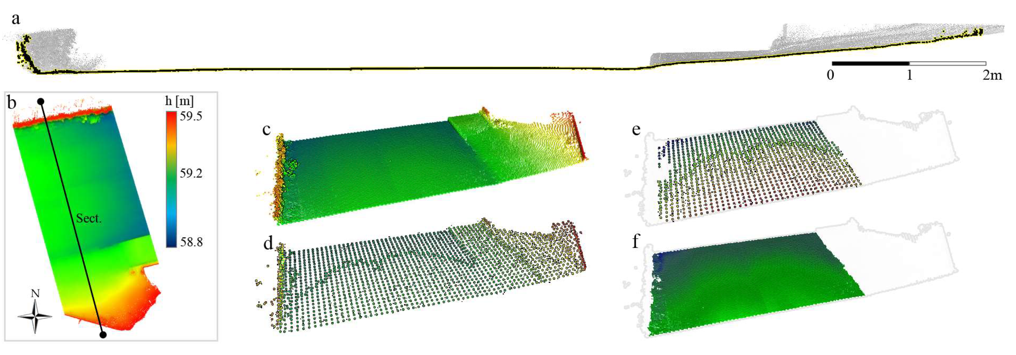
Figure 10.
Down-sampling run for a box. (a) Original point cloud, profile view along the section traced on the (b). Plan view. (c) Original point cloud. (d) Voxel grid. (e) Voxel grid after filtering. (f) Final output (filtered point cloud).
Figure 10.
Down-sampling run for a box. (a) Original point cloud, profile view along the section traced on the (b). Plan view. (c) Original point cloud. (d) Voxel grid. (e) Voxel grid after filtering. (f) Final output (filtered point cloud).

Figure 11.
(a) shows the original point cloud, the grey tones represent the intensity values. (b) The edited point cloud superimposed on the original cloud, the color gradation is proportional to the height value. (c–e) Some perspective views of the edited cloud. (c) Some objects have been removed, including a tripod. (d) A spherical target mounted on a biped has also been removed. (e) A west-east perspective view of the edited cloud superimposed on the original.

Figure 12.
Roughness values given in grey-scale tones. The graduation ranges from black (negative values) to white (positive).
Figure 12.
Roughness values given in grey-scale tones. The graduation ranges from black (negative values) to white (positive).

Figure 13.
Estimation of the accuracy of the points fitting to the plane; the computed values of Root Mean Square Error (RMSE) are associated with the points.
Figure 13.
Estimation of the accuracy of the points fitting to the plane; the computed values of Root Mean Square Error (RMSE) are associated with the points.

Figure 14.
Distresses segmentation. (a) The potholes identified. (b) The swells/shoves identified.

Figure 15.
Distresses gradually identified, as the kernel size changes. Positive values of Δh correspond to potholes and negative values to swells/shoves.
Figure 15.
Distresses gradually identified, as the kernel size changes. Positive values of Δh correspond to potholes and negative values to swells/shoves.

Figure 16.
Classification into severity levels of the identified distresses (according to Standard ASTMD6433) as the kernel size changes. (a) Potholes. (b) Swells/shoves.
Figure 16.
Classification into severity levels of the identified distresses (according to Standard ASTMD6433) as the kernel size changes. (a) Potholes. (b) Swells/shoves.

Figure 17.
Trend of the main geometrical parameters of a few distresses as the kernel size changes.

Figure 18.
‘Boundary effect’. (a) A sample of point cloud belonging to a central stretch of road; the area squared in white is the one subject to analysis; the grayscale is proportional to the roughness value Δh. (b) Classified map of the difference in roughness δh computed for the points in the white square of (a). The area within the black box is not influenced by the boundary effect, the area outside the box it is.


Table 1.
Technical data of mobile laser scanning system (MLS) Riegl VMX® 450.
| 2 × Riegl VQ-450 | |
|---|---|
| Selected Measurement Rate | 1.1 MHz |
| Selected Line Scan Speed | 400 lines/sec |
| Min range | 1.5 m |
| Max Range (for the selected rate) | 140 m (target reflectivity ρ ≥ 10%) |
| 220 m (target reflectivity ρ ≥ 80%) | |
| Accuracy (1σ) | 8 mm @ 50 m |
| Precision (1σ) | 5 mm @ 50 m |
Table 2.
Severity levels of distress as a function of the mean diameter (d) and depth.
| Potholes | |||
| Depth (mm) | 100 ≤ d ≤ 200 | 200 ≤ d ≤ 450 | 450 ≤ d ≤ 750 |
| 13 ≤ |Δh | ≤ 25 | L | L | M |
| 25 ≤ |Δh | ≤ 50 | L | M | H |
| 50 ≤ |Δh | | M | M | H |
| Swells/Shoves | |||
| Depth (mm) | 100 ≤ d ≤ 200 | 200 ≤ d ≤ 450 | 450 ≤ d |
| 5 ≤ |Δh | ≤ 19 | L | L | L |
| 19 ≤ |Δh | ≤ 38 | M | M | M |
| 38 ≤ |Δh | | H | H | H |
L = Low; M = Medium; H = High.
Table 3.
The main geometrical parameters computed for some distress examples.
| Pothole | Perimeter [dm] | Area [dm2] | Volume [dm3] | h max [cm] | Max axis [cm] | Min axis [cm] | Mean diam [cm] | Class |
| 2 | 21.1 | 22.9 | 3.8 | 3.4 | 68.7 | 44.3 | 54.0 | H |
| 3 | 30.6 | 15.4 | 2.5 | 3.1 | 92.2 | 28.4 | 44.2 | M |
| 5 | 44.4 | 62.8 | 11.1 | 3.3 | 170.8 | 59.4 | 89.4 | H |
| 6 | 26.0 | 14.9 | 2.9 | 4.2 | 91.1 | 37.3 | 43.6 | M |
| 11 | 14.3 | 10.6 | 2.6 | 3.1 | 49.5 | 29.6 | 36.8 | M |
| 14 | 17.5 | 10.6 | 2.2 | 3.8 | 69.4 | 20.3 | 36.8 | M |
| 17 | 35.3 | 42.6 | 7.8 | 3.1 | 144.5 | 45.0 | 73.6 | H |
| 19 | 14.2 | 11.7 | 1.8 | 2.2 | 44.4 | 34.4 | 38.5 | L |
| 20 | 37.0 | 76.6 | 14.3 | 3.2 | 112.2 | 99.8 | 98.8 | H |
| 27 | 19.0 | 15.7 | 2.2 | 2.3 | 76.3 | 29.0 | 44.6 | L |
| Swell/shove | Perimeter [dm] | Area [dm2] | Volume [dm3] | h max [cm] | Max axis [cm] | Min axis [cm] | Mean diam [cm] | Class |
| 10 | 27.1 | 18.9 | 1.3 | 1.4 | L | |||
| 11 | 17.7 | 13.5 | 1.2 | 1.6 | L | |||
| 16 | 73.5 | 81.5 | 5.6 | 1.5 | L | |||
| 18 | 25.6 | 17.0 | 1.0 | 1.1 | L | |||
| 19 | 35.0 | 36.8 | 2.5 | 1.2 | L | |||
| 22 | 24.5 | 15.1 | 0.9 | 1.0 | L | |||
| 24 | 44.1 | 30.6 | 1.8 | 1.1 | L | |||
| 25 | 348.5 | 351.5 | 30.6 | 1.9 | M | |||
| 35 | 123.1 | 167.3 | 12.6 | 1.5 | L | |||
| 38 | 148.0 | 289.9 | 21.7 | 1.6 | L | |||
| 45 | 170.7 | 181.2 | 14.6 | 1.6 | L | |||
| 49 | 119.7 | 128.6 | 8.6 | 1.3 | L | |||
| 53 | 16.8 | 17.1 | 1.4 | 1.4 | L | |||
| 54 | 21.5 | 16.3 | 1.1 | 1.2 | L | |||
| 57 | 113.3 | 122.9 | 13.2 | 1.9 | M | |||
| 60 | 52.5 | 52.3 | 3.3 | 1.2 | L | |||
| 66 | 80.4 | 83.3 | 5.5 | 1.3 | L | |||
| 72 | 48.9 | 27.2 | 1.7 | 1.4 | L | |||
| 73 | 40.6 | 42.0 | 2.7 | 1.2 | L | |||
| 77 | 63.2 | 75.9 | 5.6 | 1.5 | L |
© 2020 by the authors. Licensee MDPI, Basel, Switzerland. This article is an open access article distributed under the terms and conditions of the Creative Commons Attribution (CC BY) license (http://creativecommons.org/licenses/by/4.0/).
Share and Cite
MDPI and ACS Style
De Blasiis, M.R.; Di Benedetto, A.; Fiani, M. Mobile Laser Scanning Data for the Evaluation of Pavement Surface Distress. Remote Sens. 2020, 12, 942. https://0-doi-org.brum.beds.ac.uk/10.3390/rs12060942
AMA Style
De Blasiis MR, Di Benedetto A, Fiani M. Mobile Laser Scanning Data for the Evaluation of Pavement Surface Distress. Remote Sensing. 2020; 12(6):942. https://0-doi-org.brum.beds.ac.uk/10.3390/rs12060942
Chicago/Turabian StyleDe Blasiis, Maria Rosaria, Alessandro Di Benedetto, and Margherita Fiani. 2020. "Mobile Laser Scanning Data for the Evaluation of Pavement Surface Distress" Remote Sensing 12, no. 6: 942. https://0-doi-org.brum.beds.ac.uk/10.3390/rs12060942
Note that from the first issue of 2016, this journal uses article numbers instead of page numbers. See further details here.