Article

Himawari-8-Derived Aerosol Optical Depth Using an Improved Time Series Algorithm Over Eastern China

1
The School of Environment and Geoinformatics, China University of Mining and Technology, Xuzhou 221116, China
2
Jiangsu Key Laboratory of Coal-Based Greenhouse Gas Control and Utilization, China University of Mining and Technology, Xuzhou 221008, China
3
Geomatics in the School of Geoscience and Info-Physics, Central South University, Changsha 410000, China
4
Institute of Environmental Physics and Remote Sensing, University of Bremen, 28359 Bremen, Germany
5
ROyal Netherlands Meteorological Institute (KNMI), Research and Development (R&D) Satellite Observations, Utrechtseweg 297, 3731GA De Bilt, The Netherlands
6
School of Atmospheric Sciences, Nanjing University of Information Sciences and Technology, Nanjing 210044, China
*
Author to whom correspondence should be addressed.
Submission received: 13 February 2020 / Revised: 12 March 2020 / Accepted: 16 March 2020 / Published: 18 March 2020
(This article belongs to the Special Issue Active and Passive Remote Sensing of Aerosols and Clouds)

Abstract

:
Himawari-8 (H8), as a new generation geostationary meteorological satellite, has great potential for monitoring the spatial–temporal variation of aerosol properties. However, the large amount of spectral data with differing observation geometries require re-formulation of the surface reflectance correction to utilize this new satellite data. This is achieved by using an improved version of the time series (TS) technique proposed by Mei et al., (2012) based on the assumption that the ratio of the surface reflectance in different spectral bands does not change between any two scan times within an hour. In addition, more suitable aerosol models were adopted, based on cluster analysis of local Aerosol Robotic Network (AERONET) data. The improved TS algorithm (ITS) was applied to retrieve the Aerosol Optical Depth (AOD) over eastern China and the results compare favorably with collocated reference AOD data at eleven sun photometer sites (R > 0.8, Root Mean Square Error (RMSE) < 0.2). Comparison with the H8 official AOD product and with MODIS Dark Target (DT)–Deep Blue (DB) combined AOD data shows the good performance of the ITS method for AOD retrieval with different observation angles.

Graphical Abstract

1. Introduction

Aerosols are important for climate and climate change, due to their reflection and absorption of solar radiation and their effects on cloud properties [1]. They are also important for human health, especially for people with respiratory problems and lung diseases [2,3]. Furthermore, they play a role in atmospheric chemistry, while at the same time their variability is very large, which severely affects cloud microphysics [4,5]. Hence, it is important to obtain accurate information on the occurrence of aerosols and their properties. One way to obtain this information on large spatial scales is the use of satellites, using sensors with an initiative-designed task for aerosol retrieval. Many sensors designed for land and sea surface temperatures are also suitable for aerosol retrieval, such as the European Space Agency’s (ESA) along-track scanning radiometers (ATSR-2 and AATSR) [6,7,8].
Sensors suitable for aerosol retrievals are Moderate Resolution Imaging Spectroradiometer (MODIS) [9], Visible infrared Imaging Radiometer (VIIRS) [10], Polarization and Directionality of the Earth’s Reflectances (POLDER) [11] and the Chinese directional polarimetric camera (DPC) [12], with different characteristics for aerosol retrieval, such as wavebands at wavelengths ranging from the ultra-violet (UV) to the thermal infrared (TIR; MODIS, VIIRS), two or more viewing angles (ATSR, POLDER), and polarization (POLDER, DPC). All of these sensors are attached to sun-synchronous, polar-orbiting satellites, which implies that the revisit time for each point on Earth is one day or more (depending on swath width). Therefore, at best one or two observations per day are available [13,14,15]. In this study, we focus on the use of geostationary satellites, and in particular the advanced Himawari imager (AHI) onboard the Himawari-8 (H8) satellite. Geostationary satellites observe only a certain part of the earth, however at a temporal frequency of several observations each hour during the daytime. This provides information on the diurnal variation of aerosol properties, which is important for air quality studies and health effects, as well as to study aerosol transport. In the current study, we only consider aerosol retrieval over land.
Only a few algorithms have reached a state of maturity, rendering them suitable for the operational production of aerosol data and the creation of climate data records [16,17]. The most crucial issue for the retrieval of aerosol properties using passive sensors is the effective separation of the contributions from the underlying surface and atmospheric components to the reflectance measured at the top of the atmosphere (TOA), especially because the combination is nonlinear and under-constrained [18,19].
The wide variety of land surface types results in variability of the surface appearance from dark forest to bright desert, snow, or ice covered surfaces, with an associated variation of surface reflectance [20]. Due to the huge spatial–temporal variability in aerosol concentration and the complex mixing of aerosol types, aerosol retrieval is difficult [4,21,22]. Therefore, to retrieve aerosol information from satellite observations, effective separation of the surface reflectance and atmospheric path radiance contributions to the reflectance measured at the TOA is necessary. Furthermore, satellite observations do not provide enough information for a detailed characterization of the aerosol properties, and therefore assumptions of the aerosol type are required.
To effectively correct for the surface contributions to the TOA reflectance, several methods have been proposed using different assumptions. For sensors with a single view, the accuracy of the aerosol signal separated from the TOA signal is largely based on an accurate determination of the surface reflection [19,23]. For MODIS, the dark target (DT) method has been developed [24], which uses the real-time relationship between the reflectance in the visible and shortwave infrared bands over dark dense vegetation. However, the DT method applies only to a limited range of surface albedos [9], while for more reflecting surfaces other methods are needed. This idea was also later used in the retrieval of sensor Advanced Baseline Imager (ABI) (on American stationary satellite Geostationary Operational Environmental Satellites - R Series (GOES-R)) [25]. The deep blue (DB) method [26] was developed for use over brighter surfaces, which utilizes wavelengths in the UV spectral region where the surface appears dark. These methods have also been applied to other sensors, such as VIIRS, Sea-Viewing Wide Field-of-View Sensor (SeaWiFS), and Advanced Very High Resolution Radiometer (AVHRR) [27]. DB and DT data products are, in principle, complementary, covering different types of surfaces, while MODIS Collection 6 and 6.1 data product include a combined DT and DB AOD product [28,29,30]. Other methods use physical models to represent the angular variation of the surface reflectance, as described by the bidirectional reflectance distribution function (BRDF). A widely used BRDF data set is available from MODIS observations using the Ross–Li model based on images measured over 16 consecutive days [31]. For geostationary satellites, it is relatively easier to obtain enough observations. Govaerts et al. [32,33,34] used the Rahman–Pinty–Verstraete (RPV) model to simultaneously retrieve the average AOD and surface BRDF reflectance of Meteosat Second Generation–Spinning Enhanced Visible and Infra-red Imager (MSG–SEVIRI) within a day. Because of the high temporal resolution of geostationary satellites, their data can facilitate surface and aerosol research.
In the current study, we focus on the use of the H8–AHI geostationary satellite. For aerosol retrieval, Ge et al. [35] used the relationship between the reflection in the visible and mid-infrared bands of H8–AHI, following the MODIS and ABI algorithms [24,25]. However, due to the long observation period of a geostationary satellite, this method has some shortcomings in establishing a strong relationship between the surface reflectance in the visible spectral band and the TOA reflectance in the infrared band. She et al. [36] used the MODIS BRDF dataset [31] to jointly retrieve the hourly AOD and the surface reflectance, but this method also suffers from some errors due to fixing the shape of the surface BRDF. In the H8–AHI official aerosol retrieval algorithm (further referred to as the “official algorithm”), a predefined minimum surface method was used from a historical dataset with hourly equivalent BRDF information [37] (similar to Geostationary Ocean Color Imager (GOCI) [38,39]). This method may introduce some uncertainties by synthesizing the optimal albedo from historical data, resulting in obvious deviations in some areas compared with AOD measurements from AERONET sites [40,41].
In addition to surface assumptions, there are still some difficulties in deriving AOD from atmospheric signals. The aerosol microphysical parameters determine the scattering and absorption of light by particles, so the use of incorrect aerosol parameters directly leads to incorrect AOD retrievals. In general, aerosol properties can be obtained from the analysis of long-term measurements [21,32]. However, for simplicity, many algorithms use existing aerosol models and do not take into account the spatiotemporal variations of actual aerosol types [35,42].
Mei et al. [43] presented a time series (TS) method for MSG–SEVIRI data, which is based on the assumption that the surface albedo in one pixel remains unchanged during three consecutive scans. With predefined fixed aerosol types, this method obtained the AOD by utilizing a numerical minimization routine. The algorithm makes full use of the characteristics of high temporal resolution and does not need to obtain accurate surface reflectance; therefore, it can be applied to various surface types. In addition, the algorithm can also obtain the optimal aerosol type from predefined aerosol types by limiting the spatial variation of aerosol types.
In theory, the TS method is especially suitable for geostationary satellites. However, the original TS algorithm is not effective on H8–AHI due to method accuracy and inappropriate aerosol parameters [44,45,46]. Therefore, this study attempts to improve the TS algorithm in the following five aspects: (1) re-derive the basic transfer function and consider gas correction and Rayleigh scattering coupling; (2) modify the cost function to better consider the ratio of surface changes; (3) extend the observation period of the TS method to retrieve more retrievals; (4) set up aerosol models through cluster analysis to get more accurate results; (5) use optimal estimates for fast iteration with an efficient constraint. The results obtained using the improved time series (ITS) algorithm have a cross-comparison with ground-based data, the MODIS AOD product, and the H8–AHI official AOD dataset. A detailed description of the retrieval methodology is provided in Section 2, where the data are also introduced. The comparison between retrieval results is discussed in Section 3. Conclusions are presented in Section 4.

2. Retrieval Strategy and Data

2.1. Advanced Himawari Imager
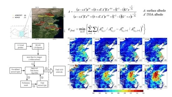
The advanced Himawari imager (AHI) is a 16-channel, multispectral imager onboard the geostationary satellite Himawari-8 (H8), developed by the Japan Meteorological Agency (JMA). H8–AHI perform full-disk observations over East Asia and the western Pacific at 10 min intervals. The first 6 bands (0.47 μm–2.2 μm) from the visible to the mid-infrared can be used to capture the radiance of atmospheric aerosols and the earth’s surface at a maximum spatial resolution of 1 kilometer in East Asia at 10 min intervals. To facilitate processing and utilization, JAXA released real-time L1B spectral data with 5 km resolution in NC format [15,47].
In the current study on the development of the ITS algorithm, we use the 5 km resolution L1B spectral dataset available from the JAXA website (http://www.eorc.jaxa.jp/ptree/index.html). Real-time L2 cloud products with the same spatial–temporal resolution are used to select cloud-free pixels [48,49]. L1B TOA albedo values at 470, 510, 640, 870, and 2250 nm measured at 10 min intervals from 09:00 to 16:00 China Standard Time (CST, i.e., UTC + 8:00) over the study area are used as input. The study period is from August 2018 to May 2019.
Complementary to satellite observations, local AOD measurements are made using ground-based sun photometers. The data from sun photometer networks, such as the global Aerosol Robotic Network (AERONET) [50,51] or the Chinese Sun–Sky Radiometer Observation Network (SONET) [52], are more accurate than satellite products, and therefore are used as a reference for the validation of satellite-retrieved AOD [35,36]. In the current study, ground-based AOD measurements from eleven AERONET and SONET sun photometer sites (see Table 1 for details) are used for validation. The four AERONET sites are Beijing-CAMS, Xianghe, Xuzhou, and Taihu. The seven SONET sites are Beijing, Yanqihu, Jiaozuo, Songshan, Hefei, Nanjing, and Shanghai. AERONET provides aerosol data at three quality levels: level 1.0 (unscreened), level 1.5 (cloud-screened and quality controlled), and level 2.0 (quality-assured) (http://aeronet.gsfc.nasa.gov). The quality of SONET AOD data corresponds to that of AERONET Level 1.5 [45,46]. Because L2.0 AERONET data for 2018 were not yet available at the time of the current study, Level 1.5 AERONET V3 AOD data were used together with corresponding SONET data.
For comparison, the H8–AHI official version 2.1 level 2.0 5km AOD product [53] and the MODIS C6.1 10 km AOD data (DT and DB combined dataset, DT–DB) from Terra and Aqua were selected. The MODIS 10 km product is widely used and can be obtained from the LAADS website (http://ladsweb.nascom.nasa.gov/data). MODIS is in a sun-synchronous polar orbit, with equator crossing times at about 10:30 (Terra satellite) and 13:30 (Aqua satellite) China Standard Time (CST).

2.2. Basic Method

The ITS algorithm needs to construct the cost function based on the surface reflectance. The ITS method uses the same two-stream approximate radiative transfer model as the original TS method (classic formula derived by Liou et al.) [54]. This model decomposes the pure atmospheric scattering processes in spherical coordinates into upward and downward flux streams ( F , F ; τ represent the atmospheric optical thickness at any position):
d F ( τ ) d τ = γ 1 F ( τ ) γ 2 F ( τ ) γ 3 ϖ F 0 exp ( τ μ 0 ) d F ( τ ) d τ = γ 2 F ( τ ) γ 1 F ( τ ) + ( 1 γ 3 ) ϖ F 0 exp ( τ μ 0 )
In Equation (1), F 0 and μ 0 represent the solar flux and cosine of its direction angle, while the coefficients γ 1 , γ 2 , γ 3 are only related to the single scattering albedo (ssa, ϖ ) and the asymmetry factor (asy, g ) of the atmosphere layer. To integrate these formulas, the boundary conditions need to be clear. Then, considering the surface albedo and the albedo at TOA, A , A , the boundary conditions for upward and downward fluxes at the top and bottom of the atmosphere are reset as Equation (2).
F ( τ = 0 ) μ 0 F 0 + F ( τ = 0 ) = A
F ( τ = 0 ) = 0
F ( τ = τ 0 ) F ( τ = τ 0 ) = A
In Equation (2), τ is the atmospheric optical depth, where F (arrow up and down with τ = 0) indicates the fluxes at TOA, and likewise F (arrow up and down with τ = τ 0 ) indicates the fluxes at the surface. Based on known boundary conditions and atmospheric parameters, the surface albedo A can be derived from TOA reflection A . After mathematical deformation and simplification, the final formula can be formulated as Equation (3):
A = ( a c A ) e k τ + ( b + c Γ A ) Γ e k τ + ( Γ 2 1 ) G + e τ μ 0 ( a c A ) Γ e k τ + ( b + c Γ A ) e k τ + ( Γ 2 1 ) ( G + c ) e τ μ 0
In Equation (3), since no new variables were introduced, a , b , c , Γ are derived from the parameters in Equation (1), so they are only related to atmospheric parameters and incident solar radiation. They are functions of the incoming solar radiation flux ( F 0 ), solar zenith angle ( μ 0 ), single scattering albedo (ssa, ω ˜ ), and asymmetry factor (asy, g ) [55,56]. All the parameters are used by Mei et al., (2012), which are the deformations of the two-stream parameters (a detailed explanation of the symbols and the equation derivation are presented in the Appendix A).
The parameters of solar flux are easily obtained, so this formula indicates that for known atmospheric parameters (aerosol and gas), the surface albedo can be calculated from the TOA reflectance measured by H8–AHI.
For a clear sky, we assume that the atmospheric optical depth ( τ ) consists of two parts (Equation (4a)): the molecular Rayleigh scattering ( τ R ) and the aerosol optical depth ( τ A ). An approximate expression for the Rayleigh scattering, Equation (4b), is sufficiently accurate for most applications in remote sensing [1]. The aerosol optical depth (AOD) varies with wavelength, as described by the Ångström turbidity Formula (4c) [1]. Over a small area and within a short period time, the aerosol properties (represented by the wavelength exponent α ) can be considered to be invariant, while the concentration of the aerosol particles (given by the Ångström turbidity coefficient β ) may change.
τ = τ A + τ R
τ R λ ( ) = 0.00879 λ 4.09
τ A = β λ α
Due to the mixing of all atmospheric particles, the optical properties of the atmospheric layer use Equations (5a) and (5b) to describe the atmospheric coupling single scattering albedo ( ω ˜ ) and coupling asymmetric factor ( g ) by optical depth weighting [57,58].
ω ˜ = ( ω ˜ A · τ A + τ R ) / ( τ A + τ R )
g = ( g A · τ A · ω ˜ A ) / ( τ A · ω ˜ A + τ R )
Additionally, gas absorption should be considered. Similar to the procedure adopted by MODIS, we use the National Centers for Environmental Prediction (NCEP) data to correct for the effect of gas absorption (H2O, CO2, and O3) on the measured TOA reflectance before retrieval is attempted [59]. The NCEP data include the 1° × 1° global meteorological analysis data. For each pixel in the L1B data, the corrected reflectance A is given by Equation (6), which has a scale factor T λ g a s based on wavelength, air mass factor, and weighting coefficients (Appendix B and Appendix C; benefiting from the similar band between AHI and MODIS, here we directly use MODIS parameter values).
A λ = T λ gas A λ L 1 B
In the case of strongly absorbing aerosols and an optically thin layer, a negative surface albedo may result from the numerical correction due to the high forward scatter peaks of atmospheric particles (an inherent defect of the two-stream approximation). Therefore, we also adjust this case by using a δ function that removes the amount of scattering of the forward peak while ensuring the consistency of parameters τ , ϖ , and g [54].

2.3. Aerosol Types

Aerosol properties are important and inappropriate aerosol type can result in inaccurate retrieval results. In the literature, different models have been proposed. For example, Govaerts et al., (2010) suggested a model consisting of six aerosol types (three for spherical and three for non-spherical particles) for use in MSG–SEVIRI AOD retrieval [32]. This model was also used by Mei et al., (2012). Derived from AERONET global data, the aerosol model used in the MODIS DT algorithm is another good model [28]. However, considering the scope of the study area, the optical properties of the global model do not agree well with local areas (Figure 1a,b). The scatterplots of the ssa versus asy at an AERONET wavelength of 675 nm, together with the values for Govaerts and MODIS aerosol models, show that these models are not completely representative for the actual aerosol properties over eastern China, especially for the absorbing spherical particles (ssa is on the edge of the cloud of data points or beyond).
Therefore, it is more suitable to construct aerosol types from long-term local measurements and accumulated meteorological data. However, a suitable aerosol model needs to consider the microphysical properties of the particles and local climatology, which is very complicated. For the two-stream approximation method in this study, the optical absorption parameter (ssa) and size parameter (asy) derived from the aerosol microphysical properties are sufficiently accurate to define different aerosol types [22,43]. Therefore, a simple k-means clustering method can be used for aerosol classification based on ssa and asy for AERONET observations in different bands. The theoretical understanding of this statistical method is incomplete; however, it can avoid explicit assumptions regarding aerosol physics in other aerosol models.
To this end, AERONET V3 level 2.0 aerosol data (best quality) at 440, 500, 675, and 870 nm spectral bands from more than 10 local AERONET sites over eastern China were collected since 2010. For ssa and asy in different bands, the k-means clustering method only needs to specify the number of types to divide the different types. Considering the average difference of each type and other models, 5 types are finally determined. For comparison, the results at 675 nm are presented in Figure 1c, with each of the five clusters coded in different colors. The values for other H8–AHI wavelengths were obtained by interpolation using quadratic fitting, which are shown in Figure 1d–f and Table 2.
In addition, AOD conversion between bands for different types can use the Ångström exponent (AE). AE is provided directly in the AERONET dataset and the highest frequency AE value in the histogram of each cluster is determined as the final AE. Using this AE value, the AOD at different wavelengths can be obtained using Equation (4c). Then, Equation (3) becomes a function that only contains AOD as unknown.

2.4. The Core Strategy

In the original TS algorithm presented by Mei et al. [1], the surface reflectance was assumed to be invariant between three consecutive observations within 30 min. There are three main disadvantages: (1) If the surface reflectance values in different bands have multiple differences, then the square sum will further expand this difference, resulting in a band with high reflectance becoming dominant in the cost function. For example, the 640 nm band of the dark pixel in the original DT algorithm is twice as large as the 470 nm band [24]. (2) The assumption of invariant surfaces leads to an uncertain time period for maintaining this invariance. In fact, although the surface reflectance changes slowly with time, it still cannot be considered constant due to the complex BRDF [33,34]. (3) Due to the cloud mask, the requirement for effective observations in three consecutive times also greatly reduces the retrieved pixels. Therefore, the cost function needs to be reconstructed.
For multi-viewing-angle instruments, the observations at different angles allow for simultaneous retrieval of surface reflectance and AOD [60]. The ratio of the directional reflectance values for different viewing directions, here referred to as the K-ratio, is approximately constant at different wavelengths [1,19,61]. This principle can also be applied to geostationary satellites based on the reflectance variation caused by different angles of the sunlight over a period of time. An effective cost function (Equation (7)) is established, from which the most suitable result should satisfy the minimum sum of differences between the K-ratios in different bands.
The cost function of ITS can be evaluated using the following equation:
ε f i n a l = min m = 5 { i = 1 n t ( A λ t 1 , i m / A λ t 2 , i m A λ t 1 , i + 1 m / A λ t 2 , i + 1 m ) 2 }
where m is the aerosol type (the total number of aerosol types is 5) defined for observations at time t 1 , t 2 (which represents any scans within one hour) and different wavebands ( i represents the spectral band, n is the total number of bands equal to 4). The different K-ratios can be calculated for different AOD combinations to determine the minimum value for the cost function ε . In this cost function, the subtractions of different K-ratios take on an order of wavelength. In fact, the pair can be arbitrarily chosen here and the result is not much different (because the values of K-ratios change slowly within an hour). By changing aerosol type, five values ε can be obtained, with the smallest one corresponding to the most probable AOD and aerosol type in the retrieval area.
In addition, by using K-ratios invariance, the observation intervals can also be expanded. The H8–AHI official document (constructed surface reflectance data set for each hour during daytime using the second minimum method) and She et al. also recommend one hour [36]. Considering the spatial–temporal variation of aerosol properties, in this paper, if there are two effective scans in an hour, Equation (6) can be used. Therefore, in the absence of sufficient observations due to the real weather, we can also get enough data. Then, an optimal constraint estimation is used to search for the best result within the bounds of real aerosol and surface conditions (assuming that the surface reflectance of the 640 nm visible band is less than the TOA reflectance of the 2250 nm middle infrared band).
The AERONET wavelengths used to define the aerosol types in this study (Figure 1 and Table 1) are close to the H8–AHI visible and NIR bands, so the optical properties ssa and asy of H8–AHI spectra (470, 510, 640, and 860 nm) can be obtained by quadratic fitting from AERONET data. For a single pixel, the selection of aerosol types may have some uncertainties due to the model accuracy, the aerosol type error, and other factors. An important constraint for the final aerosol type is used: the aerosol properties do not change during one hour and over a 1° × 1° spatial grid [22,43]. With this scheme, the aerosol type for pixels within an area can be updated by counting the aerosol type that appears most.

2.5. Execution Steps
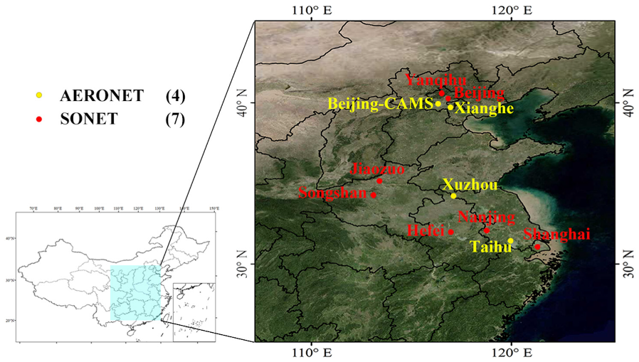
Figure 2 shows the flow chart of the ITS aerosol retrieval algorithm. For each series of cloud-free pixels from more than two H8–AHI scans within an hour, the preliminary result consists of an aerosol type, AODs, and surface albedos (for each scan), which are retrieved in steps 1 and 2. For the pixel series in each 1° × 1° grid, the most frequent aerosol type for about 400 pixels would be set as the final aerosol type for that grid (step 3). That aerosol type is used for the final processing of the 1° × 1° image (step 4) and provides the final result (step 5). This procedure imposes a spatial constraint on the aerosol types, which to some extent ensures the accuracy of the final result.

2.6. Study Area

The study area is located between 105° to 125°E and 25° to 45°N, which covers Eastern China, the Bohai Sea, and part of the Huanghai Sea (Figure 3). Many megacities are located in this area, meaning it is strongly influenced by anthropogenic atmospheric pollution [2,5]. Because of the differences between land and ocean algorithms, for this study, we only consider the retrieval of aerosols over land and validate the results by comparison with data from eleven ground-based AOD reference sites in Eastern China. The locations of these AERONET and SONET sites are marked in Figure 3 in yellow and red, respectively.

2.7. Evaluation Metrics

Spatial–temporal matching criteria are the most important criteria for the comparison of different datasets. The MODIS dataset was resampled to the same resolution as H8–AHI (5 km) by using the nearest neighbor interpolation method. However, the AODs from the MODIS product and the ITS-derived AODs are retrieved at 550 nm, the H8–AHI official product is retrieved at 519 nm, and both are different from the wavelength of the ground-based reference data. Therefore, all AOD data were converted to 0.55 µm using Equation (3c). For the convenience of comparison, the overpass times of MODIS Terra and Aqua were defined to 10:30 CST and 13:30 CST (slightly different from the actual local time).
The AOD retrieved for one pixel using the ITS method is only related to the reflectance of that same pixel in two consecutive moments, which is independent of other surrounding pixels. In order to verify the collocations from different datasets accurately, a spatial–temporal matching method used the average values of ground-based measurements during a certain time period (10 min, ± 5 min around the satellite overpass time) and the average of the satellite-retrieved AOD over an area of 5 × 5 pixels around the sun photometer site (for stability, more than 10 valid values in 25 pixels were included the calculation) was used [10,43].
For the evaluation of the H8–AHI ITS algorithm, scatterplots were made of the retrieved AOD versus reference AOD data. Four parameters were used as metrics to evaluate the performance of the ITS method: (i) the correlation coefficient (R); (ii) the percentage of ITS retrievals falling within the expected error (EE) ( ± ( 0.05 + 0.15 τ ) ), which applies to MODIS data over land and has been adopted by others [9,10]; (iii) mean difference ( M D = ( τ r e t r i e v e d τ g r o u n d b a s e d ) / n describes the mean bias between two datasets; (iv) root mean square error ( R M S E = ( τ r e t r i e v e d τ g r o u n d b a s e d ) 2 / n ) refers to the satellite product’s absolute deviation from ground-based AOD).

3. Results and Analysis

3.1. Validation against AERONET Measurements

Scatterplots of satellite-retrieved AOD products versus collocated ground-based AOD data are presented in Figure 4. For comparison, the H8–AHI L2 official AOD product is shown in the left column, the MODIS product is shown in the middle column, and the ITS method is shown in the right column. Overall, the three datasets compare favorably with the ground-based reference measurements. However, at most sites, the data retrieved using the ITS algorithm have better correlation and lower RMSE than the official H8–AHI product, and at all sites more collocations fall within the EE than the official H8–AHI product. The results from the ITS algorithm are overall not as good as those from MODIS, but at some sites (Nanjing, Taihu, and Shanghai) the ITS statistics are better than those from MODIS.
The official algorithm has taken into account the hourly BRDF characteristics, but the result is the worst in the three datasets with small correlation coefficients (often <0.8) and large RMSEs (>0.32). Especially at Yanqihu, Beijing, Beijing-CAMS, and Xianghe sites, the official product at low AOD (AERONET AOD<0.15) is much too high. In these cases, the results from the ITS method are much better than those from the official product, with a smaller number of overestimations, a larger R (>0.8), and a smaller RMSE (<0.20). Because both algorithms use the same cloud screening product, cloud contamination cannot be the reason for the higher AOD of the official product. Levy et al., (2010) concluded that surface assumptions tend to dominate AOD retrieval when there is low aerosol loading (AOD<0.15) [9]. Therefore, we conclude that the surface albedo assumption with the constant K-ratio used in the ITS algorithm provides a better surface correction than the minimum reflectance method used in the official product. However, as mentioned in Table 1, the underlying surface of Beijing and Beijing-CAMS belongs to the urban surface, whereas the Yanqihu and Xianghe sites are located in rural areas.
For Beijing and Beijing-CAMS, the ITS method partially overestimates the AOD (which is not encountered in other sites with an urban underlying surface, such as Jiaozuo and Shanghai), indicating that the surface correction in the ITS method may need further consideration. At the Xuzhou site, the distributions of three datasets are similar and the correlation coefficient of H8–AHI official product is larger than that for the ITS and MODIS. However, the collocations from ITS have the smallest RMSE and more collocations fall in the EE lines. Except for the two sites in Beijing, the ITS-derived data from other sites have a similar distribution (the upper or lower deviations of the EE envelope) from the MODIS product. When the underlying surface is a different type, there is no significant difference in the results, which indicates that the ITS algorithm can successfully retrieve AOD irrespective of surface type and the aerosol model is representative of the actual situation. H8–AHI provides much more data than MODIS due to the high temporal frequency, which fully reflects the advantages of the ITS algorithm applied to geostationary satellites. At the Taihu site, due to the weather, the number of successful retrievals from the ITS algorithm is less than that from the official product because two validated cloud-free pixels are needed in one hour. This results in the rejection of more pixels than the H8–AHI official method, which uses a single cloud-free observation.

3.2. Time Series Analysis

The frequent observations of geostationary satellites allow for monitoring of the diurnal evolution of the AOD. Figure 5 shows the AOD time series over a period of several days for selected sites, and for one site (Taihu) a full-time series of about 3 months. To this end, collocations between three satellite datasets and ground-based observations were selected from Figure 4, for which large numbers of AOD retrievals with different aerosol loading rates are available. The data in Figure 5 show that for different aerosol loadings, the ITS-derived AOD generally traces the ground-based observations well. Absolute differences are less than 0.2 and vary throughout the day. This indicates that the algorithm can capture small aerosol changes that vary with solar irradiation and the different underlying surfaces.
At the Beijing-CAMS (panel a) and Xianghe (panel b) sites, the performances of the H8–AHI official product and ITS method are different from those shown in Figure 4. The official product has a large overestimation under low aerosol loading, which is also reflected in Figure 5. Although the reference data show an almost constant AOD, those from the official product increase substantially with time and remain high. This indicates that the surface hypothesis and aerosol type used in the official algorithm do not always provide the correct result. In contrast, the ITS-derived AODs at the Beijing site are often closer to the reference, although high AOD is also observed in that data. At the Xianghe site, the ITS-derived AOD traces the reference data quite well and deviations are small, regardless of the level of aerosol loading. This illustrates the applicability of the ITS algorithm for multiple surface types. However, the performance in Beijing indicates that the ITS algorithm still needs to be further processed under some complex surfaces.
The Jiaozuo site (line c) is located in another urban area. Compared with Beijing, the AODs derived by the ITS agree well with the ground-based observations, and the daily variation is very smooth. This indicates that the ITS algorithm has a good performance, which it also has over some urban surfaces.
For the Taihu site, a full time series of about 3 months (4 August to 10 October 2018) is presented. The performance of the H8–AHI official algorithm is good at the Taihu site, with more successful retrievals than the ITS method. The ITS-derived AOD and the official product both trace the reference data well, often with a small underestimation by the ITS and a larger overestimation by the official product.

3.3. Spatial–Temporal Distributions of ITS-Derived Data

Maps of the AOD over eastern China, derived using the ITS method, are shown in Figure 6 for each hour from 09:00 to 16:00 LST on October 04, 2018. The maps show the spatial variation over the study area and the evolution during the day, with a strong increase shown over almost the whole study area, and in particular over the North China Plain. This fully demonstrates the advantages of geostationary satellites for aerosol research.

3.4. Comparison with Official H8–AHI and MODIS AOD Products

This section focuses on the spatial distribution of the ITS-retrieved AOD and its performance compared with that from the H8–AHI official product and the MODIS products. AOD maps for each of these three products, retrieved from observations on October 5, 2018, during the time of the Terra and Aqua overpasses (about 10:30 and 13.30 CST, respectively), are presented in Figure 7. Seasonal mean results including September and October 2018 are compared in Figure 8. The spatial distributions of the three datasets in Figure 7 show similar patterns but the values are very different. At 10:30 CST, the coverage of the official product (panel b) is very sparse. In contrast, in the afternoon, the H8–AHI official product (panel e) AOD is much larger than that from the ITS or MODIS. ITS-derived AOD (c and f) is much closer to the MODIS AOD (a and d), although somewhat lower. The aggregated data of the three dataset the MODIS Aqua overpass time (about 13:30 CST) can further exhibit the difference. To calculate the means, only the pixels for which the number of retrievals is larger than 2 (at least two cloud-free days) were used to calculate the monthly means. The ITS and MODIS AOD mean maps show a similar spatial pattern, while the AOD of the official product is overall much higher. This observation is consistent with the scatterplots in Figure 4. Comparison of the ITS-derived AOD maps with those from MODIS shows a qualitative similar spatial distribution, however the ITS-derived AOD is somewhat lower and patchier. This may be due to the internal accuracy difference of the two-stream model in the ITS algorithm.
For further comparison of the ITS-derived AOD and the MODIS product, the pixel-by-pixel differences between the ITS and Terra (about 10:30 CST) products are plotted in Figure 9a, while the difference plot for ITS Aqua (about 13:30 CST) is presented in Figure 9b. Figure 9a shows that in the northern part of the study area, the ITS-derived AOD is generally higher than the MODIS AOD, whereas in the southern part of the area the ITS-derived AOD is smaller. Some areas are slightly overvalued (red), but undervalued areas (blue) are more common. The coverage of positive and negative biases does not have a clear range boundary or trend between morning and afternoon. The scatterplots in Figure 9c shows that the bulk of the data is centered around the identity line, indicating good quantitative agreement between ITS and MODIS Terra for AOD up to about 0.5. However, large deviations occur, especially overestimation by a factor of 2–3. The comparison with MODIS Aqua is much lower; especially for low AOD, the ITS-derived results have an obvious underestimation and there seems to be little relation between the ITS and MODIS Aqua AOD during the afternoon overpass. The difference in the performance of the ITS algorithm between the morning and afternoon indicates that further improvements need to be made.

3.5. Aerosol Type Analysis

The ITS method can simultaneously retrieve AOD and aerosol-type products (from five predefined types). Most aerosol retrievals focus on AOD accuracy [10,62], but aerosol-type products are also a research topic [60,63,64]. In this section, the preliminary results from the ITS method are discussed.
With the two-stream approximate method in the ITS algorithm, different aerosol types can be retrieved for adjacent pixels with similar aerosol loading (accuracy limitations). This is physically not acceptable, and therefore for each 1° × 1° grid cell the aerosol type, which occurs in the largest number of pixels, is selected as the most probable type for that grid cell. It appears that most of the time and in most areas, moderately absorption (type 3; Figure 1 and Table 1) occurs most frequently. This type also occurs most frequently according to AERONET statistics. This may be due to the relatively small study area where anthropogenic aerosols dominate.
Figure 10 shows the time series of three aerosol parameters (AOD, ssa, and asy at 670 nm) derived from AERONET measurements and retrieved by the ITS algorithm for single pixels at the Beijing site. The quality of the ITS dataset at this site is not as good as other sites (Figure 4), which is representative of studying the relationship between aerosol types and AOD. Overall, the ITS-derived AODs have a qualitatively similar variation to the AERONET data. The most corresponding points, where ssa is equal to 0.953 and asy is equal to 0.653, belong to the third type. The largest differences between the ITS and AERONET AOD occur when the ssa and asy are also different from the reference data, such as on January 9 and February 28. The AOD variation is similar to that of the reference AERONET data, however the AOD values diverge when the ssa deviation is small and asy deviation is large, such as the date before January 17 and the period between February and March. When ssa and asy are in good agreement with the actual aerosol properties from ground-based measurements, this also applies to ITS-derived AOD (after March).
As expected, the aerosol type directly affects the accuracy of the AOD retrievals. As shown in Figure 10 (top panel), the ITS-derived AODs do not compare well with the reference data until February, whereas after February the comparison is good and the ITS AOD traces the AERONET AOD. The overestimation in the winter may be due to the bright surface at that time of the year, together with low AOD, as observed by AERONET [9]. During episodes with higher AOD, the ITS data compare favorably with the AERONET data.

4. Discussion and Conclusion

H8–AHI, which has an unprecedented high temporal resolution, has the capability to capture the dynamic variations of aerosols, and thus provide an important contribution to atmospheric environmental monitoring [65,66]. The use of H8–AHI data for aerosol retrieval requires an effective separation of the effects of the surface and the atmosphere, with the reflectance measured by the sensor at the top of the atmosphere. To this end, the use of a fast and accurate algorithm derived by Mei et al., (2012) was proposed and further improvements were made for use with H8–AHI data. Compared with the official algorithm and the MODIS DT algorithm, this algorithm can make full use of the characteristics of geostationary satellites. The generic nature of this algorithm renders it suitable for real-time operational use. Simultaneously retrieved aerosol types give the algorithm wider application prospects. Validation with independent reference data from AERONET and comparison with MODIS AOD show the good performance at the ITS-retrieved AOD. The ITS algorithm performance is better than that of the current official H8–AHI aerosol product (smaller RMSE and more points within the EE at all sites) and close to the MODIS product. The aerosol models are used in the algorithms, which were developed for this area using the clustering method for AERONET data in the study area. The evaluation of the retrieved aerosol types shows a good agreement between the retrieval aerosol type and the real aerosol type.
However, improvements to this new algorithm are still needed. Comparison with AERONET measurements at the Beijing-CAMS and Beijing sites shows an obvious overestimation at low aerosol loading (AOD<0.2), although the ITS results are better than the official product. Additionally, the ITS performs better at other urban sites than at the Beijing sites. This may be explained from the residual contribution of the surface albedo and the differences in retrieval algorithms between ground-based instruments and satellite sensors (which may be insensitive to very thin aerosol layers [54]). The overestimation of the AOD for low aerosol loading at the Beijing sites has also been reported in other studies [35,36] and requires further analysis. In addition, because this algorithm uses only two effective scans in an hour, it lacks a strict surface constraint over one or more days [67].
The use of accurate aerosol types is crucial. The aerosol type retrieved by the ITS algorithm has a good correlation with the real situation, and the influence of the absorption as expressed by the ssa and the asy on AOD was found (Figure 10). However, this algorithm only considers these two parameters, so it should be improved in the future to cover a variety of atmospheric properties for a specific area, such as eastern China [62]. On the other hand, the degrees of freedom available from satellite observations are insufficient to provide detailed information on the aerosol properties, which may lead to a simple formulation of aerosol models, providing a priori estimates, which are refined in the retrieval processing using the observations at different wavelengths [33,34].
The uncertainty factors mentioned above will be addressed in a future study to improve the performance of the ITS algorithm for atmospheric monitoring using the H8–AHI satellite.

Author Contributions

Data curation, D.L., Y.L., and Y.S.; methodology, D.L. and L.M.; investigation and simulations, writing—original draft preparation, D.L. and K.Q.; writing—review and editing, G.d.L. and Y.X.; supervision, L.W. All authors have read and agreed to the published version of the manuscript.

Acknowledgments

This work was funded by the National Natural Science Foundation of China (Grant No. 41975041). The authors thank the AERONET principal investigators and site managers who provided the data. The authors are grateful to Aerospace Information Research Institute (AIR) of the Chinese Academy of Sciences (CAS) for providing the ground-based sun photometer measurements. We would also like to acknowledge Japan Aerospace Exploration Agency for providing the datasets (available from: ftp://ftp.ptree.jaxa.jp) and NASA for providing MODIS AOD datasets (available from: https://ladsweb.modaps.eosdis.nasa.gov).

Conflicts of Interest

The authors declare no conflict of interest.

Abbreviations

SymbolDescription
F ( τ ) Total upward flux densities with atmosphere optical depth equal to τ
F ( τ ) Total downward flux densities with atmosphere optical depth equal to τ
F 0 Solar flux density at the top of atmosphere
μ 0 Cosine of solar zenith angle
A ( A λ )Earth’s surface reflectance (at λ spectral band)
A ( A λ )Earth’s system reflectance (at λ spectral band)
τ , τ 0 Total optical depth
τ A Aerosol optical depth
τ R Rayleigh optical depth
g , g Asymmetry factor
ϖ , ϖ Single scattering albedo
α Wavelength exponent in angstrom’s turbidity formula
β Angstrom’s turbidity coefficient
T λ g a s Atmospheric gas transmission factor
m Number of predefined aerosol types
n Number of bands
θ , θ 0 View zenith angle, solar zenith angle

Appendix A. Symbols in Equation (2)

a = G + G Γ b = G G + Γ c = F 0 μ 0 Γ = γ 1 k γ 2 G + = μ 0 2 ϖ F o ( k μ 0 ) 2 1 [ ( γ 1 1 μ 0 ) γ 3 + γ 2 γ 4 ] G = μ 0 2 ϖ F 0 ( k μ 0 ) 2 1 [ ( γ 1 + 1 μ 0 ) γ 4 + γ 2 γ 3 ] k 2 = γ 1 2 γ 2 2 F 0 = S ( r 0 r ) 2 μ 0 μ 1 = 0.5774 γ 1 = 1 μ 1 [ 1 ω ˜ 2 ( 1 + g ) ] γ 2 = ω ˜ 2 μ 1 ( 1 g ) γ 3 = 1 2 ( 1 3 g μ 1 μ 0 )
Reference: Mei et al., (2012) [1], Liou et al., (2004) [54].

Appendix B. Symbols in Equation (5).

T λ g a s = T λ C O 2 T λ O 3 T λ H 2 O G = 1 cos ( θ 0 ) + 1 cos ( θ ) T λ H 2 O = exp ( exp ( K 1 , λ H 2 O + K 2 , λ H 2 O ln ( G w ) + K 3 , λ H 2 O ( ln ( G w ) ) 2 ) ) T λ H 2 O = exp ( G τ λ H 2 O ¯ ) T λ O 3 = exp ( G K λ O 3 O ) T λ O 3 = exp ( G τ λ O 3 ¯ ) T λ C O 2 = exp ( G τ λ C O 2 ¯ )

Appendix C

Table A1. The appropriate coefficients for each gas.
Wavelength K 1 ,   λ H 2 O K 2 ,   λ H 2 O K 3 ,   λ H 2 O τ λ H 2 O K λ O 3 τ λ O 3 τ λ C O 2
0.47 4.26 × −62.432 × −3
0.55 1.05 × −42.957 × −2
0.66−5.7390.926−0.0191.543 × −25.09 × −52.478 × −2
0.86−5.3300.824−0.0281.947 × −2
Reference: Xue et al. (2014) [1], Levy et al. (2013) [28].

References

  1. Xue, Y.; He, X.; Xu, H.; Guang, J.; Guo, J.; Mei, L. China Collection 2.0: The aerosol optical depth dataset from the synergetic retrieval of aerosol properties algorithm. Atmos. Environ. 2014, 95, 45–58. [Google Scholar] [CrossRef]
  2. Wu, L.; Lü, X.; Qin, K.; Bai, Y.; Li, J.; Ren, C.; Zhang, Y. Analysis to Xuzhou aerosol optical characteristics with ground-based measurements by sun photometer. Kexue Tongbao/Chinese Sci. Bull. 2016, 61, 2287–2998. [Google Scholar]
  3. Qin, K.; Wang, L.; Wu, L.; Xu, J.; Rao, L.; Letu, H.; Shi, T.; Wang, R. A campaign for investigating aerosol optical properties during winter hazes over Shijiazhuang, China. Atmos. Res. 2017, 198, 113–122. [Google Scholar] [CrossRef]
  4. Gultepe, I.; Isaac, G.A. Scale effects on averaging of cloud droplet and aerosol number concentrations: Observations and models. J. Clim. 1999, 12, 1268–1279. [Google Scholar] [CrossRef]
  5. Qin, K.; Wu, L.; Man, S.W.; Letu, H.; Hu, M.; Lang, H.; Sheng, S.; Teng, J.; Xiao, X.; Yuan, L. Trans-boundary aerosol transport during a winter haze episode in China revealed by ground-based Lidar and CALIPSO satellite. Atmos. Environ. 2016, 141, 20–29. [Google Scholar] [CrossRef] [Green Version]
  6. Veefkind, J.P.; De Leeuw, G.; Durkee, P.A. Aerosol optical depth retrieval over land from two angle view satellite radiometry. J. Aerosol Sci. 1998, 29, 65–74. [Google Scholar]
  7. Kolmonen, P.; Sogacheva, L.; Virtanen, T.H.; de Leeuw, G.; Kulmala, M. The ADV/ASV AATSR aerosol retrieval algorithm: Current status and presentation of a full-mission AOD dataset. Int. J. Digit. Earth 2016, 9, 545–561. [Google Scholar] [CrossRef]
  8. Sogacheva, L.; Rodriguez, E.; Kolmonen, P.; Virtanen, T.H.; Saponaro, G.; De Leeuw, G.; Georgoulias, A.K.; Alexandri, G.; Kourtidis, K.; Van Der, R.J.A. Spatial and seasonal variations of aerosols over China from two decades of multi-satellite observations—Part 2: AOD time series for 1995-2017 combined from ATSR ADV and MODIS C6.1 and AOD tendency estimations. Atmos. Chem. Phys. 2018, 18, 16631–16652. [Google Scholar] [CrossRef] [Green Version]
  9. Levy, R.C.; Remer, L.A.; Kleidman, R.G.; Mattoo, S.; Ichoku, C.; Kahn, R.; Eck, T.F. Global evaluation of the Collection 5 MODIS dark-target aerosol products over land. Atmos. Chem. Phys. 2010, 10, 10399–10420. [Google Scholar] [CrossRef] [Green Version]
  10. Xiao, Q.; Zhang, H.; Choi, M.; Li, S.; Kondragunta, S.; Kim, J.; Holben, B.; Levy, R.C.; Liu, Y. Evaluation of VIIRS, GOCI, and MODIS Collection 6 AOD retrievals against ground sunphotometer observations over East Asia. Atmos. Chem. Phys. 2016, 16, 1255–1269. [Google Scholar] [CrossRef] [Green Version]
  11. Hou, W.; Li, Z.; Wang, J.; Xu, X.; Goloub, P.; Qie, L. Improving remote sensing of aerosol microphysical properties by near-infrared polarimetric measurements over vegetated land: Information content analysis. J. Geophys. Res. Atmos. 2018, 123, 2215–2243. [Google Scholar] [CrossRef]
  12. Li, Z.; Hou, W.; Hong, J.; Zheng, F.; Luo, D.; Wang, J.; Gu, X.; Qiao, Y. Directional Polarimetric Camera (DPC): Monitoring aerosol spectral optical properties over land from satellite observation. J. Quant. Spectrosc. Radiat. Transf. 2018, 218, 21–37. [Google Scholar] [CrossRef]
  13. Kim, J.; Yoon, J.M.; Ahn, M.H.; Sohn, B.J.; Lim, H.S. Retrieving aerosol optical depth using visible and mid-IR channels from geostationary satellite MTSAT-1R. Int. J. Remote Sens. 2008, 29, 6181–6192. [Google Scholar] [CrossRef]
  14. Seo, S.-B.; Lim, H.-S.; Ahn, S.-I. Introduction to image pro-processing subsystem of geostationary ocean color imager (GOCI). Korean J. Remote Sens. 2010, 26, 167–173. [Google Scholar]
  15. Bessho, K.; Date, K.; Hayashi, M.; Ikeda, A.; Imai, T.; Inoue, H.; Kumagai, Y.; Miyakawa, T.; Murata, H.; Ohno, T. An introduction to himawari-8/9—Japan’s new-generation geostationary meteorological satellites. J. Meteorol. Soc. Jpn. Ser. II 2016, 94, 151–183. [Google Scholar] [CrossRef] [Green Version]
  16. De Leeuw, G.; Holzer-Popp, T.; Bevan, S.; Davies, W.H.; Descloitres, J.; Grainger, R.G.; Griesfeller, J.; Heckel, A.; Kinne, S.; Klüser, L.; et al. Evaluation of seven European aerosol optical depth retrieval algorithms for climate analysis. Remote Sens. Environ. 2015, 162, 295–315. [Google Scholar] [CrossRef] [Green Version]
  17. Popp, T.; De Leeuw, G.; Bingen, C.; Brühl, C.; Capelle, V.; Chedin, A.; Clarisse, L.; Dubovik, O.; Grainger, R.; Griesfeller, J.; et al. Development, production and evaluation of aerosol climate data records from European satellite observations (Aerosol_cci). Remote Sens. 2016, 8, 421. [Google Scholar] [CrossRef] [Green Version]
  18. Martonchik, J.V.; Kahn, R.A.; Diner, D.J. Retrieval of aerosol properties over land using MISR observations. In Satellite Aerosol Remote Sensing Over Land; Springer: Berlin, Germany, 2009; pp. 267–293. [Google Scholar]
  19. Xue, Y.; Cracknell, A.P. Operational bi-angle approach to retrieve the earth surface albedo from AVHRR data in the visible band. Int. J. Remote Sens. 1995, 16, 417–429. [Google Scholar] [CrossRef]
  20. Yan, X.; Li, Z.; Luo, N.; Shi, W.; Zhao, W.; Yang, X.; Jin, J. A minimum albedo aerosol retrieval method for the new-generation geostationary meteorological satellite Himawari-8. Atmos. Res. 2018, 207, 14–27. [Google Scholar] [CrossRef]
  21. Dubovik, O.; Holben, B.; Eck, T.F.; Smirnov, A.; Kaufman, Y.J.; King, M.D.; Tanré, D.; Slutsker, I. Variability of absorption and optical properties of key aerosol types observed in worldwide locations. J. Atmos. Sci. 2002, 59, 590–608. [Google Scholar] [CrossRef]
  22. Levy, R.C.; Remer, L.A.; Dubovik, O. Global aerosol optical properties and application to Moderate Resolution Imaging Spectroradiometer aerosol retrieval over land. J. Geophys. Res. Atmos. 2007, 112. [Google Scholar] [CrossRef] [Green Version]
  23. Mei, L.L.; Xue, Y.; Kokhanovsky, A.A.; Von Hoyningen-Huene, W.; De Leeuw, G.; Burrows, J.P. Retrieval of aerosol optical depth over land surfaces from AVHRR data. Atmos. Meas. Tech. 2014, 7, 2411–2420. [Google Scholar] [CrossRef] [Green Version]
  24. Remer, L.A.; Kaufman, Y.J.; Tanré, D.; Mattoo, S.; Chu, D.A.; Martins, J.V.; Li, R.-R.; Ichoku, C.; Levy, R.C.; Kleidman, R.G.; et al. The MODIS aerosol algorithm, products, and validation. J. Atmos. Sci. 2005, 62, 947–973. [Google Scholar] [CrossRef] [Green Version]
  25. Center for Satellite Applications and Research (Star), Noaa Nesdis. ABI Aerosol Detection Product. Available online: https://www.star.nesdis.noaa.gov/goesr/documents/ATBDs/Baseline/ATBD_GOES-R_Aerosol_Detection_v3.0_Jan2019.pdf (accessed on 18 March 2020).
  26. Hsu, N.C.; Jeong, M.-J.; Bettenhausen, C.; Sayer, A.M.; Hansell, R.; Seftor, C.S.; Huang, J.; Tsay, S.-C. Enhanced deep blue aerosol retrieval algorithm: The second generation. J. Geophys. Res. Atmos. 2013, 118, 9296–9315. [Google Scholar] [CrossRef]
  27. Shen, S.; Sayer, A.M.; Bettenhausen, C.; Wei, J.C.; Ostrenga, D.M.; Vollmer, B.E.; Hsu, N.Y.; Kempler, S.J. Global Long-Term SeaWiFS Deep Blue Aerosol Products available at NASA GES DISC. In Proceedings of the Agu Fall Meeting, San Francisco, CA, USA, 3–7 December 2012. [Google Scholar]
  28. Levy, R.C.; Mattoo, S.; Munchak, L.A.; Remer, L.A.; Sayer, A.M.; Patadia, F.; Hsu, N.C. The Collection 6 MODIS aerosol products over land and ocean. Atmos. Meas. Tech. 2013, 6, 2989–3034. [Google Scholar] [CrossRef] [Green Version]
  29. Jing, W.; Lin, S.; Bo, H.; Bilal, M.; Zhang, Z.; Wang, L. Verification, improvement and application of aerosol optical depths in China Part 1: Inter-comparison of NPP-VIIRS and Aqua-MODIS. Atmos. Environ. 2018, 175, 221–233. [Google Scholar]
  30. Wei, J.; Li, Z.; Peng, Y.; Sun, L. MODIS Collection 6. 1 aerosol optical depth products over land and ocean: Validation and comparison MODIS Collection 6. 1 aerosol optical depth products over land and ocean: Validation and comparison. Atmos. Environ. 2018, 201, 428–440. [Google Scholar] [CrossRef]
  31. Strahler, A.H.; Muller, J.P.; Lucht, W.; Schaaf, C.; Tsang, T.; Gao, F.; Li, X.; Lewis, P.; Barnsley, M.J. MODIS BRDF/albedo product: Algorithm theoretical basis document version 5.0. MODIS Doc. 1999, 23, 42–47. [Google Scholar]
  32. Govaerts, Y.M.; Wagner, S.; Lattanzio, A.; Watts, P. Joint retrieval of surface reflectance and aerosol optical depth from MSG/SEVIRI observations with an optimal estimation approach: 1. Theory. J. Geophys. Res. 2010, 115. [Google Scholar] [CrossRef]
  33. Govaerts, Y.; Luffarelli, M. Joint retrieval of surface reflectance and aerosol properties with continuous variation of the state variables in the solution space--Part 1: Theoretical concept. Atmos. Meas. Tech. 2018, 11, 6589–6603. [Google Scholar] [CrossRef]
  34. Luffarelli, M.; Govaerts, Y. Joint retrieval of surface reflectance and aerosol properties with continuous variation of the state variables in the solution space-Part 2: Application to geostationary and polar-orbiting satellite observations. Atmos. Meas. Tech. 2019, 12, 791–809. [Google Scholar] [CrossRef] [Green Version]
  35. Ge, B.; Li, Z.; Liu, L.; Yang, L.; Chen, X.; Hou, W.; Zhang, Y.; Li, D.; Li, L.; Qie, L. a dark target method for himawari-8/ahi aerosol retrieval: application and validation. IEEE Trans. Geosci. Remote Sens. 2018, 57, 381–394. [Google Scholar] [CrossRef]
  36. She, L.; Xue, Y.; Yang, X.; Leys, J.; Guang, J.; Che, Y.; Fan, C.; Xie, Y.; Li, Y. Joint retrieval of aerosol optical depth and surface reflectance over land using geostationary satellite data. IEEE Trans. Geosci. Remote Sens. 2019, 57, 1489–1501. [Google Scholar] [CrossRef]
  37. Kikuchi, M.; Murakami, H.; Suzuki, K.; Nagao, T.M.; Higurashi, A. Improved hourly estimates of aerosol optical thickness using spatiotemporal variability derived from Himawari-8 geostationary satellite. IEEE Trans. Geosci. Remote Sens. 2018, 56, 3442–3455. [Google Scholar] [CrossRef]
  38. Choi, M.; Kim, J.; Lee, J.; Kim, M.; Park, Y.-J.; Jeong, U.; Kim, W.; Hong, H.; Holben, B.; Eck, T.F.; et al. GOCI Yonsei Aerosol Retrieval (YAER) algorithm and validation during the DRAGON-NE Asia 2012 campaign. Atmos. Meas. Tech. 2016, 9, 1377–1398. [Google Scholar] [CrossRef] [Green Version]
  39. Choi, M.; Kim, J.; Lee, J.; Kim, M.; Park, Y.-J.; Holben, B.; Eck, T.F.; Li, Z.; Song, C.H. GOCI Yonsei aerosol retrieval version 2 products: An improved algorithm and error analysis with uncertainty estimation from 5-year validation over East Asia. Atmos. Meas. Tech. 2018, 11, 385–408. [Google Scholar] [CrossRef] [Green Version]
  40. Lim, H.; Choi, M.; Kim, M.; Kim, J.; Chan, P.W. Retrieval and validation of aerosol optical properties using Japanese next generation meteorological satellite, Himawari-8. Korean J. Remote Sens. 2016, 32, 681–691. [Google Scholar] [CrossRef] [Green Version]
  41. Li, D.; Qin, K.; Wu, L.; Xu, J.; Letu, H.; Zou, B.; He, Q.; Li, Y. Evaluation of JAXA Himawari-8-AHI level-3 aerosol products over eastern China. Atmosphere 2019, 10, 215. [Google Scholar] [CrossRef] [Green Version]
  42. Xue, Y.; He, X.; de Leeuw, G.; Mei, L.; Che, Y.; Rippin, W.; Guang, J.; Hu, Y. Long-time series aerosol optical depth retrieval from AVHRR data over land in North China and Central Europe. Remote Sens. Environ. 2017, 198, 471–489. [Google Scholar] [CrossRef]
  43. Mei, L.; Xue, Y.; de Leeuw, G.; Holzer-Popp, T.; Guang, J.; Li, Y.; Yang, L.; Xu, H.; Xu, X.; Li, C.; et al. Retrieval of aerosol optical depth over land based on a time series technique using MSG/SEVIRI data. Atmos. Chem. Phys. 2012, 12, 9167–9185. [Google Scholar] [CrossRef] [Green Version]
  44. Hongbin, W.; Lei, Z.; Shengming, J.; Zhiwei, Z.; Yuying, Z.H.U.; Chengying, Z.H.U. Evaluation of the MODIS aerosol products and analysis of the retrieval errors in China. Plateau Meteorol. 2016, 35, 810–822. [Google Scholar]
  45. Li, Z.; Zhang, Y.; Xu, H.; Li, K.; Dubovik, O.; Goloub, P. The fundamental aerosol models over china region: A cluster analysis of the ground-based remote sensing measurements of total columnar atmosphere. Geophys. Res. Lett. 2019, 46, 4924–4932. [Google Scholar] [CrossRef]
  46. Li, L.; Zheng, X.; Li, Z.; Li, Z.; Dubovik, O.; Chen, X.; Wendisch, M. Studying aerosol light scattering based on aspect ratio distribution observed by fluorescence microscope. Opt. Express 2017, 25, A813–A823. [Google Scholar] [CrossRef] [PubMed] [Green Version]
  47. Kikuchi, M.; Murakami, H.; Nagao, T.; Yoshida, M.; Nio, T.; Oki, R. EarthCARE and Himawari-8 Aerosol Products EarthCARE. 2016. Available online: http://icap.atmos.und.edu/ICAP8/Day3/Kikuchi_JMA_ThursdayAM.pdf (accessed on 18 March 2020).
  48. Shang, H.; Chen, L.; Letu, H.; Zhao, M.; Li, S.; Bao, S. Development of a daytime cloud and haze detection algorithm for Himawari-8 satellite measurements over central and eastern China. J. Geophys. Res. Atmos. 2017, 122, 3528–3543. [Google Scholar] [CrossRef]
  49. Letu, H.; Nagao, T.M.; Nakajima, T.Y.; Riedi, J.; Ishimoto, H.; Baran, A.J.; Shang, H.; Sekiguchi, M.; Kikuchi, M. Ice cloud properties from Himawari-8/AHI next-generation geostationary satellite: Capability of the AHI to monitor the DC cloud generation process. IEEE Trans. Geosci. Remote Sens. 2018, 57, 3229–3239. [Google Scholar] [CrossRef]
  50. Holben, B.; Slutsker, I.; Giles, D.; Eck, T.; Smirnov, A.; Sinyuk, A.; Schafer, J.; Sorokin, M.; Rodriguez, J.; Kraft, J.; et al. AERONET Version 3 Release: Providing Significant Improvements for Multi-Decadal Global Aerosol Database and Near Real-Time Validation, Nasa Technical Reports. 2016. Available online: https://ntrs.nasa.gov/search.jsp?R=20160013870 (accessed on 30 January 2020).
  51. Giles, D.M.; Sinyuk, A.; Sorokin, M.G.; Schafer, J.S.; Smirnov, A.; Slutsker, I.; Eck, T.F.; Holben, B.N.; Lewis, J.R.; Campbell, J.R.; et al. Advancements in the Aerosol Robotic Network (AERONET) Version 3 database—Automated near-real-time quality control algorithm with improved cloud screening for Sun photometer aerosol optical depth (AOD) measurements. Atmos. Meas. Tech. 2019, 12, 169–209. [Google Scholar] [CrossRef] [Green Version]
  52. Ie, Y.; Li, Z.; Li, D.; Xu, H.; Li, K. Aerosol optical and microphysical properties of four typical sites of SONET in China based on remote sensing measurements. Remote Sens. 2015, 7, 9928–9953. [Google Scholar]
  53. JAXA Earth Observation Research Center (EORC). JAXA Himawari Monitor Aerosol Products. Available online: https://www.eorc.jaxa.jp/ptree/documents/Himawari_Monitor_Aerosol_Product_v6.pdf (accessed on 17 April 2019).
  54. Liou, K.N. An Introduction to Atmospheric Radiation/Kuo-Nan Liou; Elsevier: Amsterdam, The Netherlands, 2002. [Google Scholar]
  55. Meador, W.E.; Weaver, W.R. Two-stream approximations to radiative transfer in planetary atmospheres: A unified description of existing methods and a new improvement. J. Atmos. Sci. 1980, 37, 630–643. [Google Scholar] [CrossRef] [Green Version]
  56. Higurashi, A.; Nakajima, T. Development of a two-channel aerosol retrieval algorithm on a global scale using noaa avhrr. J. Atmos. Sci. 1999, 56, 924–941. [Google Scholar] [CrossRef]
  57. Zhang, F.; Shen, Z.; Li, J.; Zhou, X.; Ma, L.-M. Analytical delta-four-stream doubling–adding method for radiative transfer parameterizations. J. Atmos. Sci. 2013, 70, 794–808. [Google Scholar] [CrossRef]
  58. Wu, K.; Zhang, F.; Min, J.; Yu, Q.-R.; Wang, X.-Y.; Ma, L. Adding method of delta-four-stream spherical harmonic expansion approximation for infrared radiative transfer parameterization. Infrared Phys. Technol. 2016, 78, 254–262. [Google Scholar] [CrossRef]
  59. Falguni, P.; Levy, C.R.; Shana, M. Correcting for trace gas absorption when retrieving aerosol optical depth from satellite observations of reflected shortwave radiation. Atmos. Meas. Tech. 2018, 11, 3205–3219. [Google Scholar]
  60. Dubovik, O.; Herman, M. Statistically optimized inversion algorithm for enhanced retrieval of aerosol properties from spectral multi-angle polarimetric satellite observations. Atmos. Meas. Tech. 2010, 4, 975–1018. [Google Scholar] [CrossRef] [Green Version]
  61. Flowerdew, R.J.; Haigh, J.D. Retrieval of aerosol optical thickness over land using the ATSR-2 Dual-Look satellite radiometer. Geophys. Res. Lett. 1996, 23, 351–354. [Google Scholar] [CrossRef]
  62. De Leeuw, G.; Sogacheva, L.; Rodriguez, E.; Kourtidis, K.; Georgoulias, A.K.; Alexandri, G.; Amiridis, V.; Proestakis, E.; Marinou, E.; Xue, Y.; et al. Two decades of satellite observations of AOD over mainland China using ATSR-2, AATSR and MODIS/Terra: Data set evaluation and large-scale patterns. Atmos. Chem. Phys. 2018, 18, 1573–1592. [Google Scholar] [CrossRef] [Green Version]
  63. Kahn, R.A.; Garay, M.J.; Nelson, D.L.; Levy, R.C.; Tanré, D. Response to toward unified satellite climatology of aerosol properties. 3. modis versus misr versus aeronet. J. Quant. Spectrosc. Radiat. Transf. 2011, 112, 901–909. [Google Scholar] [CrossRef] [Green Version]
  64. Kahn, R.A.; Gaitley, B.J. An analysis of global aerosol type as retrieved by MISR. J. Geophys. Res. Atmos. 2015, 120, 4248–4281. [Google Scholar] [CrossRef]
  65. Uesawa, D. Aerosol Optical Depth product derived from Himawari-8 data for Asian dust monitoring. Meteorol. Satell. Cent. Tech. 2016, 59, 59–63. [Google Scholar]
  66. Wang, W.; Mao, F.; Du, L.; Pan, Z.; Gong, W.; Fang, S. Deriving hourly PM2.5 concentrations from Himawari-8 AODs over Beijing-Tianjin-Hebei in China. Remote Sens. 2017, 9, 858. [Google Scholar] [CrossRef] [Green Version]
  67. Lyapustin, A.; Wang, Y.; Korkin, S.; Huang, D. MODIS Collection 6 MAIAC algorithm. Atmos. Meas. Tech. 2018, 11, 5741–5765. [Google Scholar] [CrossRef] [Green Version]
Figure 1. Three aerosol types (panel (a) for Govaerts’ model, panel (b) for MODIS, panel (c,df) for cluster types at different bands). The Aerosol Robotic Network (AERONET)-derived data are plotted as the small background points, while the larger colored dots represent different aerosol types.
Remotesensing 12 00978 g001
Figure 2. Flow chart for the improved time series (ITS) aerosol retrieval algorithm. See text for explanation of the various steps. AOD, aerosol optical depth; H8–AHI, Himawari-8–advanced Himawari imager.
Remotesensing 12 00978 g002
Figure 3. Study area over eastern China. Locations and names of reference sites are indicated in yellow (AERONET) and red (SONET).
Remotesensing 12 00978 g003
Figure 4. Color scatterplots of aerosol optical depth (AOD) from the H8–AHI official product (left), the MODIS AOD product (middle), and the ITS method (right) against ground-based reference AOD measurements at six sites (each row represents one site) from August to December 2018. The color bar indicates the number of data points, the red solid line is linear regression, the gray solid line is the 1:1 line, and the dashed blue lines are the expected error (EE) envelopes. N means the number and other meaning of the text in the legends has been described in Section 2.7.
Remotesensing 12 00978 g004aRemotesensing 12 00978 g004b
Figure 5. Comparison of AOD retrieved using the ITS method (red), the H8–AHI official product (blue), the MODIS product (black star), and AERONET observations (green) for four different AERONET sites (indicated at the top right of each panel). The top three panels show only a few days each, whereas the bottom panel (Taihu) shows all retrieved AOD values over about 3 months (August to October) in 2018.
Remotesensing 12 00978 g005
Figure 6. ITS-retrieved AOD maps on October 04, 2018, for 8 consecutive hours from 09:00 to 16:00.
Remotesensing 12 00978 g006
Figure 7. AOD maps derived from the MODIS Terra and Aqua products (panel (a,d)), the H8–AHI official product (b,e), and the ITS method (panel (c,f)) on October 05, 2018, at 10:30 China Standard Time (CST; top) and 13:30 CST (bottom).
Remotesensing 12 00978 g007
Figure 8. AOD maps aggregated for September and October 2018 from the MODIS Aqua datasets (panel (a,d)), the H8–AHI official product (b,e), and the ITS method (c,f) at 13:30 pm, CST.
Remotesensing 12 00978 g008
Figure 9. (a) difference maps of the ITS and MODIS AOD on October 05, 2018. (b) scatterplots of ITS-derived AOD vs. MODIS Terra (c) and MODIS Aqua (d).
Remotesensing 12 00978 g009
Figure 10. Time series of three aerosol parameters (AOD (top), single scattering albedo (ssa) and asymmetry factor (asy) (bottom) at 670 nm) retrieved from H8–AHI data using the ITS algorithm (red) and from AERONET inversions (green) from January to May 2019 at the Beijing site. The ITS-derived ssa has been color coded according to the aerosol type (types 1–5, see legend).
Remotesensing 12 00978 g010
Table 1. Locations of the eleven sun photometer sites used in the current study, including the surface type and period for which data were available.
SitesLongitude (°)Latitude (°)Altitude (m)PeriodSurface
Beijing-CAMS116.3839.98922018.8–2019.05Urban
Beijing116.3840.01592018.8–2019.05Urban
Xianghe116.9639.75362018.8–2019.05Rural
Xuzhou117.1434.22602018.8–2019.05Suburb
Taihu120.2231.42202018.8–2018.10Urban
Yanqihu116.6740.411002018.8–2019.05Rural
Jiaozuo113.2535.191132018.8–2019.05Urban
Songshan113.1034.544752018.8–2019.05Woodland
Hefei117.1631.91362018.8–2019.05Suburb
Nanjing118.9632.12522018.8–2019.05Suburbs
Shanghai121.4831.28852018.8–2019.05Urban
Table 2. Aerosol types resulting from the cluster analysis described in the text: single scattering albedo values (ssa, ω ˜ ) and asymmetry parameters (asy, g ) at four different wavelengths.
Model
ω ˜ / g
470 nm510 nm640 nm870 nm
10.941/0.7430.946/0.7360.963/0.7110.962/0.696
20.839/0.6970.83/0.6880.814/0.6640.785/0.659
30.944/0.700.946/0.6890.953/0.6530.947/0.632
40.89/0.7040.891/0.6960.895/0.6720.88/0.66
50.895/0.6730.897/0.660.904/0.6180.889/0.60

