The Delineation and Grading of Actual Crop Production Units in Modern Smallholder Areas Using RS Data and Mask R-CNN

Abstract

The extraction and evaluation of crop production units are important foundations for agricultural production and management in modern smallholder regions, which are very significant to the regulation and sustainable development of agriculture. Crop areas have been recognized efficiently and accurately via remote sensing (RS) and machine learning (ML), especially deep learning (DL), which are too rough for modern smallholder production. In this paper, a delimitation-grading method for actual crop production units (ACPUs) based on RS images was explored using a combination of a mask region-based convolutional neural network (Mask R-CNN), spatial analysis, comprehensive index evaluation, and cluster analysis. Da’an City, Jilin province, China, was chosen as the study region to satisfy the agro-production demands in modern smallholder areas. Firstly, the ACPUs were interpreted from perspectives such as production mode, spatial form, and actual productivity. Secondly, cultivated land plots (C-plots) were extracted by Mask R-CNN with high-resolution RS images, which were used to delineate contiguous cultivated land plots (CC-plots) on the basis of auxiliary data correction. Then, the refined delimitation-grading results of the ACPUs were obtained through comprehensive evaluation of spatial characteristics and real productivity clustering. For the conclusion, the effectiveness of the Mask R-CNN model in C-plot recognition (loss = 0.16, mean average precision (mAP) = 82.29%) and a reasonable distance threshold (20 m) for CC-plot delimiting were verified. The spatial features were evaluated with the scale-shape dimensions of nine specific indicators. Real productivities were clustered by the incorporation of two-step cluster and K-Means cluster. Furthermore, most of the ACPUs in the study area were of a reasonable scale and an appropriate shape, holding real productivities at a medium level or above. The proposed method in this paper can be adjusted according to the changes of the study area with flexibility to assist agro-supervision in many modern smallholder regions.

1. Introduction

With population growth and social development, sustainable agriculture has become one of focuses of international communities [1,2]. The requirements for agricultural fine regulation are thus increasing. The accurate identification and extraction of crop production units are the basis of agricultural supervision and management. In areas with a high degree of agricultural modernization, production units are mainly crop areas (CAs) [3,4] with scale-mechanized production and modern management. With the development of remote sensing (RS) and image processing technologies, especially deep learning (DL), an effective way to monitor CAs has been provided. However, in modern smallholder areas (e.g., some regions in China) [5], the agricultural scale and level of modernization are relatively low, and production heterogeneity is high within CAs because of complex reasons. CAs are too coarse to be regarded as actual production units. Therefore, dividing and evaluating actual production units using RS and DL are the keys to accurately determine actual crop productivity in modern smallholder areas. In this way, scientific supervision and guidance can be realized.

Until now, the combinations of RS and DL have shown higher performance in studies related to agro-production units than traditional methods. Relevant studies have mainly focused on CA mapping [6,7], crop classification [8,9,10,11,12,13,14,15], and crop yield estimation [16], which are all done at the pixel level. Castro et al. [15] proved that convolutional neural networks (CNNs) and autoencoders (AEs) outperform the traditional approaches for crop classification on multi-temporal optical data and synthetic aperture radar (SAR) images. IKussul et al. [14] proposed a multilevel DL architecture with geospatial data post-processing for crop classification, whose accuracy was higher than 85% with multi-temporal Landsat-8 and Sentinel-1A images. Ji et al. [13] described a three-dimensional (3D) CNN with an active learning strategy to improve the automatic classification of crops from spatio-temporal GF-1/2 images. La Rosa et al. [12] presented a dense fully convolutional network (dense FCN) for crop classification with SAR image sequences. Zhong et al. [11] developed a one-dimensional convolutional (Conv1D) layer based classification framework using a time series enhanced vegetation index (EVI) calculated by Landsat data for classifying summer crops. Zhao et al. [10] separately combined one-dimensional (1D) CNNs, long short-term memory (LSTM) recurrent neural networks (RNNs), and gated recurrent unit (GRU) RNNs with an incremental classification method to classify early crops with Sentinel-1A image sequences. Zhou et al. [9] improved parcel-based crop classification with multi-temporal ZY-3 and Sentinel-1 images, in which spatial features were extracted and organized with multiple deep convolutional networks (DCNs) and LSTM. Cué La Rosa et al. The authors of [8] confirmed the effectiveness of DL (AEs, CNN, and FCN) for crop recognition based on multi-temporal Sentinel-1 images. However, the research on modern smallholder areas is still in its infancy. Du et al. [7] demonstrated the effectiveness of using a deep semantic segmentation network in crop region mapping with WorldView-2 and DeepLabv3+. Wei et al. [6] proposed applying U-Net for large-scale crop mapping with analysis of variance (ANOVA) and Jeffries–Matusita (J–M) distance to optimize multi-temporal Sentinel-1 images. These studies still fail to correspond to the productive process or to refine the actual production unit level.

In recent years, the agricultural scale and modernization in modern smallholder areas have been improved through land circulation [17], land consolidation, etc. The corresponding actual production unit is between the C-plot and CA. Only a few relevant studies exist [18,19]; these studies mainly proceed from farmers’ production demands rather than the requirements of agricultural supervision. Considering the difficulties in defining production units and supervising precision agriculture in modern smallholder areas, actual crop production unit (ACPU) is proposed in this paper. The output and process state of agro-production were particularly important in the ACPU’s conception. The ACPU is a set of spatially connected and form-similar cultivated land plots (C-plots) with basically uniform production modes, including cultivated land type, planting structure, tillage methods and processes, utilization intensity, agro-techniques, field management, etc. The actual productivity of each C-plot intra-ACPU is similar while the inter-ACPU is different. Even though DL with RS data is considered to be the most promising method to recognize and grade ACPUs, the process was decomposed in consideration of the related complicated factors, spatial analysis, complex calculations, and subjective decisions. In this process, C-plot recognition is the key that requires not only the total range of cultivated land but also clear individual boundaries. However, the inter-class boundaries and intra-class individuals cannot be taken into account at the same time in most DL algorithms. Thus, instance segmentation was used in this paper. At present, the leading architectures mainly include fully convolutional instance-aware semantic segmentation (FCIS) [20], mask region-based convolutional neural network (Mask R-CNN) [21], path aggregation network (PANet) [22], Mask^X R-CNN [23], hybrid task cascade (HTC) [24], and deep instance co-segmentation by co-peak search and co-saliency detection (DeepCO3) [25]. The training speed of FCIS is fast, but its performance against overlapping targets is unstable. The feature information propagation path in Mask R-CNN is improved by PANet, but PANet is not open source, and has limited applications. The advantages of a hybrid cascading structure and semantic segmentation are combined in HTC. Nevertheless, the HTC is complex and inflexible. Based on Mask R-CNN, the range of recognizable types is greatly expanded by Mask^X R-CNN, while the requirement for the samples’ mask is decreased. However, Mask^X R-CNN does not conform to C-plot application scenarios. Moreover, Mask^X R-CNN is not open source. The interactive information and segmentation mask of instance objects repeatedly appearing in images can be obtained by DeepCO3 without training samples, but the content and instance types of images should be as simple as possible. As a milestone, Mask R-CNN offers stable performance [26], a simple structure, and good generalization ability. Thus, Mask R-CNN was ultimately selected as the instance segmentation algorithm in this paper.

Li et al. [27] proposed an algorithm based on Mask R-CNN to recognize the operational behavior of pigs with an accuracy of 94.5%. Qiao et al. [26] achieved cattle instance segmentation and contour extraction using Mask R-CNN. The mean pixel accuracy (MPA) of segmentation was 92%, and the average distance error (ADE) of contour extraction was 33.56 pixels. Yu et al. [28] proposed a strawberry detection algorithm with Mask R-CNN. The average detection precision was 95.78%, and the mean intersection over the union (MIOU) was 89.85%. Lin et al. [29] combined migration learning and Mask R-CNN to classify rice planthoppers with average recognition accuracy of 92.3%. Stewart et al. [30] trained a Mask R-CNN model to segment northern leaf blight disease lesions in unmanned aerial vehicle (UAV) images, for which the MIOU was 73% and the average precision was 96%. Lu et al. [31] developed a Mask R-CNN model to localize lettuce and segment leaf areas with an average precision of 97.63%. Li et al. [32] extracted individual pigs by Mask R-CNN; the segmentation accuracy and MPA were 94.92% and 83.83%, respectively. Overall, the agricultural applications of Mask R-CNN are still in their nascent stages. The study objects were mostly individual fruits, plants, or livestock, and the study goals were mainly form, behavior, growth, and lesions. Mask R-CNN has not been used for C-plot recognition. Thus, a meaningful attempt, applying Mask R-CNN to C-plot recognition, is presented in this paper.

Da’an City, Jilin Province, China, was chosen as the study area. In this study, we proposed a combinatorial method to achieve the delimitation and grading of ACPUs in modern smallholder areas, based on RS images, preprocessing (sample preparation, image computation, etc.), and a union of Mask R-CNN with traditional technologies (post-classification processing, spatial analysis, comprehensive index evaluation, cluster analysis, etc.). The structure of following article is as follows: Section 2 describes the basic situation of the research area and data acquisition; Section 3 introduces all the methods and principles used in this paper; Section 4 presents the experimental results, analysis, and discussion; and Section 5 summarizes the research conclusions.

2. Study area and data

2.1. Study area

Da’an City lies in a geographical range of 123°8′–124°22′E and 44°57′–45°46′N in the World Geodetic System 1984 (WGS84). It is located in the northwest of Jilin Province, China, and in the hinterland of Songnen Plain (Figure 1). Da’an City has a population of more than 430,000, occupying approximately 4879 km². The terrain of whole study region is low and flat, with an elevation almost in the range of 120–160 m. Cultivated land resources account for 30% of the total area and are mainly distributed in the north and central areas, 90% of which is protected by Chinese laws. Da’an City is an important commodity grain base for China and is located in a globally famous gold corn-belt. However, the average area of household cultivated land is less than 1.67 ha. Salinized land accounts for 51.49% of the total area, of which moderate–severe salinized land makes up 66%. Da’an City is a typical area with limited agricultural resource supplies.

Da’an City has a temperate, semi-arid continental monsoon climate with four distinct seasons [33]. Spring is dry and windy. Summer is hot with concentrated precipitation. Autumn is cool with a large temperature difference. Winter is cold and dry. The average annual precipitation is 415.7 mm and the average annual evaporation is 951.2 mm, which does not support rain-fed agriculture. The annual average temperature is 4.3 °C. The difference of the average daily temperature between the warmest month and the coldest month is above 42 °C. A variety of soil types are distributed in Da’an City [34]. Chernozem and meadow soil are the major soil types. The main crops in Da’an City are corn, rice, soybean, and sorghum. At present, Da’an City has become one of China’s typical modern smallholder economic areas and modern agricultural core potential regions, for which research on precision agriculture supervision is important.

2.2. Data acquisition

According to the research process, the basic data for preparing the C-plot instance samples included digital orthophoto map (DOM) (2 × 2 m) and a land use change survey vector database (V-database) from the Da’an City Land Use Change Survey in 2016 and the Landsat 8 OLI images of the crop’s flourishing period in 2016. The scale of V-database is 1:10,000. The V-database was not only the main reference for drawing C-plot samples, but also an important basis for revising the segmentation results. The land use change survey data were taken from the Natural Resources Bureau of Da’an City. The RS base map for instance segmentation was formed by DOM and Landsat 8 OLI images: (1) The Landsat 8 images were pre-processed and resampled. (2) The resampled near-infrared band (2 × 2 m) of Landsat 8 and the red and green bands of DOM were extracted and composited to 3-band images with false colors.

Landsat 8 images were used to calculate the vegetation indexes (VIs) at the C-plot level. The local crop’s flourishing period is mainly from August to September. Two periods of images were selected to be merged and applied, which were photographed on August 28 and September 20, 2016. In this paper, five VIs including normalized difference vegetation index (NDVI), green normalized difference vegetation index (GNDVI), ration vegetation index (RVI), transformed vegetation index (TVI), and vegetation condition index (VCI), were selected and calculated (see

Table 1. Vegetation indexes (VIs) and calculation principle.

VI	Formula	Interpretation
Normalized difference vegetation index (NDVI) [35]	$\mathrm{NDVI}=\frac{{\rho }_{NIR}-{\rho }_r}{{\rho }_{NIR}+{\rho }_r}$	${\rho }_{NIR}$: near-infrared reflectance value; ${\rho }_r$: red reflectance value; ${\rho }_g$: green reflectance value; $NDV{I}_{min}$: NDVI’s multi-year minimum value of each pixel; $NDV{I}_{max}$: NDVI’s multi-year maximum value of each pixel
Green normalized difference vegetation index (GNDVI) [36]	$\mathrm{GNDVI}=\frac{{\rho }_{NIR}-{\rho }_g}{{\rho }_{NIR}+{\rho }_g}$
Ration vegetation index (RVI) [37]	$\mathrm{RVI}=\frac{{\rho }_{NIR}}{{\rho }_r}$
Transformed vegetation index (TVI) [38]	$\mathrm{TVI}=\sqrt{NDVI+0.5}$
Vegetation condition index (VCI) [39]	$\mathrm{VCI}=\frac{NDVI-NDV{I}_{min}}{NDV{I}_{max}-NDV{I}_{min}}$

). These five VIs are all commonly used and effective indicators for crop yield predictions, vegetation coverage detection, and vegetation status monitoring [35,36,37,38,39], which are suitable for situations with high vegetation coverage and dense vegetation growth. In the research process, these five VIs were highly available, of which the computation results had much spatial variability and difference information.

The pre-processing (including collection, screening, matching, mosaic, clipping, etc.) and VI calculation of the Landsat 8 images was undertaken on the Google Earth Engine (GEE, https://earthengine.google.com/) platform. GEE is a cloud-based platform for geospatial analysis, archiving a large catalog of earth observation data and supporting various pixel-based supervised and unsupervised classifiers to monitor or map multi-temporal land-use and land-cover change (LUCC), including machine learning [40,41,42,43]. GEE is suitable for large-scale data processing, greatly reducing space and time requirements [44].

3. Methods

The main flow of this paper includes two blocks (Figure 2): (1) recognizing the C-plots of the study area using the instance segmentation approach and (2) delineating and grading ACPUs through analyses of spatial features and real productivity. Instance segmentation combines the advantages of semantic segmentation and object detection. The location and category of each object can be determined to achieve individual recognition based on classification.

To recognize individual C-plots, this process involved three parts: (1) collecting and preparing the data (Landsat 8 OLI images, DOM, V-database, RS base image, VIs dataset, etc.) for instance segmentation and subsequent productivity analysis, following the procedures described in the data acquisition section; (2) achieving the instance segmentation of C-plots with Mask R-CNN using the above RS base image, of which the process included three stages. The first was the training stage: using Google Earth and V-database as the ground truth, a unified sample set was obtained through image segmentation, visual interpretation, manual labeling, format transformation, data augmentation, etc. The training set was randomly extracted from the sample set in a certain proportion and fed into the Mask R-CNN to train the model. The parameters of the model were adjusted by the loss function and gradient descent method through an iterative process. The second was the model accuracy verification stage: for the trained model, the inference mean average precision (mAP) of the test set and the loss value from the training stage were calculated. The third was the prediction and recognition stage: pre-processed image plots of the whole study area were fed into the trained model to generate the primary recognition results of the C-plots; (3) obtaining the final recognition results of the C-plots from the primary results by classification post-processing with reference to V-database. This process mainly included spatial analysis, vectorization, etc.

The delineation and grading of ACPUs entailed three steps: (1) obtaining the primary delineation results of ACPUs. First, the optimal distance threshold for merging C-plots was determined by experiments and comparisons to form the primary results of the contiguous cultivated land plots (CC-plots). Second, the primary results of the CC-plots were corrected by barrier factor patches in the V-database to obtain the preliminary delineation results of the ACPUs; (2) obtaining the primary delineation-grading results of ACPUs using a comprehensive index evaluation of the spatial characteristic indicator system. The indicator system was built from ACPU’s definition; (3) obtaining the final delineation-grading results of the ACPUs. Some studies have shown that various VIs are effective representations of real agro-productivity, crop yield, and crop growth status [45,46,47]. The actual crop production capacities could be characterized by the consistency of multiple aspects of crop growth states at pivotal time periods, which were used as the evidence for refining the ACPUs. Thus, the VIs of C-plots were clustered and analyzed to obtain the final delineation-grading results of the ACPUs, by two-step cluster and K-Means cluster.

3.1. Instance segmentation of C-plots

3.1.1. Network structure and working process of Mask R-CNN

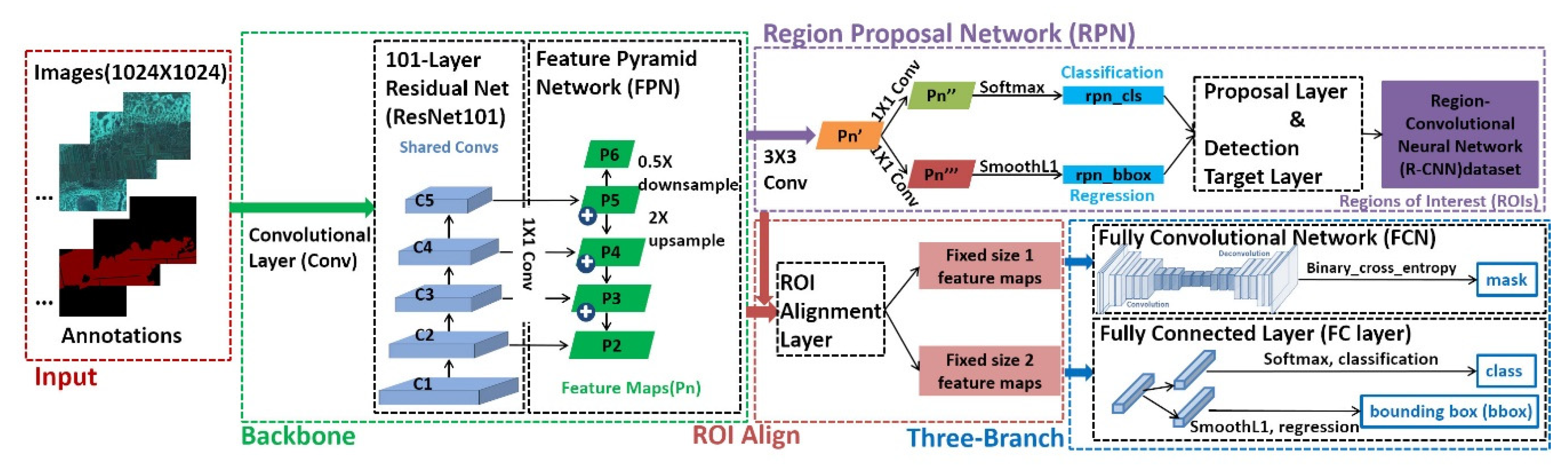
Mask R-CNN is developed from Faster Region-Convolutional Neural Networks (Faster R-CNN) [48,49], and Faster R-CNN is inherited from Fast Region-Convolutional Neural Networks (Fast R-CNN) [50]. Fast R-CNN is formed on the basis of Region-Convolutional Neural Networks (R-CNN) [51]. The architecture of Mask R-CNN is shown in Figure 3, including the feature extraction module, region proposal network (RPN), the region of interest (ROI) alignment layer, the classification-regression-mask prediction module (three-branch module), etc.

The backbone of the feature extraction module is a 101-layer residual net (ResNet101) [52], while the framework includes feature pyramid networks (FPN) [53]. The essence of ResNet101 is a series of shared convolutional layers (Shared Convs) that are used to extract multi-layer feature maps of the input images from the bottom-up. The bottom-up process is a common forward propagation for extracting feature maps using neural networks. The convolution kernels in a neural network are usually arranged from a large size to a small size in the same order as the convolution computation process. The FPN is a network connection form for combining and enhancing the semantic information in multi-layer feature maps, which is effective for solving multi-scale problems in object detection. The process of FPN has three steps: (1) the nearest neighbor up-sample is carried out for every layer except the 1st and 2nd based on a multi-layer feature map from ResNet101; (2) the up-sample results are horizontally connected to the Conv1D [54] results of the upper layer for summation. Conv1D means a one-dimensional convolution, which is used for parameter reduction and data simplification in a neural network; (3) the nearest neighbor down-sample is carried out for the last layer. As a result, the feature pyramid is constructed so that each feature layer features strong semantic and spatial information.

Based on the FPN, ROIs are generated by two sub-modules (classification and regression) of the RPN. The purpose of the RPN is to identify the possible targets, while specific types are temporarily ignored. The processing steps are as follows: (1) traversing each pixel in every feature layer to generate the anchors per center pixel. An anchor is a rectangular target box on the corresponding center pixel on a feature map. The target box is an optional item of object detection. The area of the anchor is determined by the corresponding feature map, which is equal to the square value of the relative step size between the feature map and the original image. There are three anchors generated on each central pixel with three horizontal-vertical ratios of 0.5, 1, and 2. Then, the anchors are divided into positive and negative classes with a ratio of about 1:1 according to the threshold screening of the intersection over union (IOU). The IOU is calculated between each anchor and ground truth box:

$$IOU=\frac{area{{\displaystyle \cap }}^{}are{a}^{*}}{area{{\displaystyle \cup }}^{}are{a}^{*}}$$

(1)

where $area$ and $are{a}^{*}$ represent the predicted area and the ground truth area, respectively; (2) for the positive and negative anchors, the foreground or background score of every anchor and coordinate offset between each anchor and the corresponding ground truth are calculated by forward propagation; (3) updating the weights of the network by back propagation. For the classification sub-module, the binary cross-entropy loss of the Softmax function is adopted in the RPN:

$$S_j=\frac{e^{a_j}}{{\sum }_{k=1}^T{e}^{a_k}}$$

(2)

$$L_{RPN1}=-{\displaystyle \sum }_{j=1}^T{Q}_j\log S_j$$

(3)

where $a_j$ represents the score of category $j$ calculated through network forward propagation; $T$ is the total number of categories; $S_j$ expresses the probability of category $j$ covered by the Softmax function; $L_{RPN1}$ means the classification loss of RPN; and $Q_j$ stands for the true class label. The difference between $S_j$ and $Q_j$ is calculated as a gradient of each feature layer when $L_{RPN1}$ is transmitted back, and is used to guide the weight parameter update of the network at the next forward propagation. For the bounding box (bbox) regression sub-module, the loss function of the Smooth_L1 function is employed in RPN, whose derivative is used to guide the weight updating of the feature layer:

$$Smoot{h}_{L1}=\{\begin{array}{c}0.5x^2 if\left|x\right|<1\\ \left|x\right|-0.5 otherwise\end{array}$$

(4)

$$L_{RPN2}={\displaystyle \sum }_{i\in \left\{x,y,w,h\right\}}Smoot{h}_{L1}\left(t_i-{t_i}^{*}\right)$$

(5)

$$t_x=\frac{x-x_a}{w_a},t_y=\frac{y-y_a}{h_a},t_w=\log \frac{w}{w_a},t_h=\log \frac{h}{h_a}$$

(6)

$${t_x}^{*}=\frac{x^{*}-x_a}{w_a},{t_y}^{*}=\frac{y^{*}-y_a}{h_a},{t_w}^{*}=\log \frac{w^{*}}{w_a},{t_h}^{*}=\log \frac{h^{*}}{h_a}$$

(7)

where $L_{RPN2}$ expresses the bbox regression loss of RPN; $\mathrm{x}$/$\mathrm{y}$/$\mathrm{w}$/$\mathrm{h}$, ${\mathrm{x}}_{\mathrm{a}}$/${\mathrm{y}}_{\mathrm{a}}$/${\mathrm{w}}_{\mathrm{a}}$/${\mathrm{h}}_{\mathrm{a}}$, and ${\mathrm{x}}^{*}$/${\mathrm{y}}^{*}$/${\mathrm{w}}^{*}$/${\mathrm{h}}^{*}$, respectively, represent the coordinates of the prediction box calculated by forward propagation, the anchor and truth box; $t_i=\left\{t_x,t_y,t_w,t_h\right\}$ is a vector that stands for the offset between the anchor and prediction box from RPN; ${t_i}^{*}$ is a vector that has the same dimension as $t_i$ and indicates an offset between the anchor and truth box. (4) On the proposal layer, a number of anchors at the top of the list are considered to be ROIs in descending order of foreground scores. The coordinates of the ROIs are adjusted to obtain more accurate prediction boxes by offset from forward propagation. Redundant boxes are removed by non-maximum suppression (NMS) to obtain the final ROIs. (5) On the detection target layer, the truth boxes containing multiple objects are deleted. The IOUs between the retained ROIs and truth boxes are calculated, while the ROIs are divided into positive samples and negative samples by the IOU threshold. For each positive sample, the category, regression offset and mask information from the closest truth box are calculated to form the R-CNN dataset.

The ROI alignment layer is used to map every ROI to a multi-layer feature map according to uniform alignment rules: (1) determining the corresponding feature layer of each ROI through the width-height size; (2) defining the relevant step size from the corresponding feature layer; (3) calculating the mapping size of the ROI to the feature layer based on the width-height size of the ROI and the step size from the feature layer; (4) setting the fixed alignment rules, where the mapping result on the feature layer per ROI is split, recombined, and interpolated to receive the corresponding fixed size feature map and to meet the input requirements of the subsequent fully connected layer (FC layer).

The three-branch module consists of a classification-bbox regression branch and a mask prediction branch. The former is similar to the classification-regression principle in RPN. The difference is that there are only two categories (foreground and background) in RPN, while the three-branch module has more categories. The latter is described below. Based on the results of the RPN and ROI alignment layer, for every ROI, (1) forward propagation is used to obtain the prediction masks of various categories using the deconvolution of the fixed size feature maps with FCN; (2) categories and mask information are returned by the R-CNN dataset and are used as the truth masks for various categories; (3) after assigning the per-prediction mask to the appropriate category, the final prediction results of the mask are output with the weight update guided by reverse propagation using the average binary cross-entropy loss:

$$L_{mask}=-{\displaystyle \sum }_{i=1}^n\widehat{y_i}\log y_i+(1-\widehat{y_i})\log (1-\widehat{y_i})$$

(8)

$$\frac{\partial L_3}{\partial y}=-{\displaystyle \sum }_{i=1}^n\frac{\widehat{y_i}}{y_i}-\frac{1-\widehat{y_i}}{1-y_i}$$

(9)

where $y_i$ indicates prediction probability calculated from a per-pixel sigmoid; $\widehat{y_i}$ is the true class label; and $\widehat{y_i}$ expresses the pixel number per ROI. The mask branch outputs a T × M² matrix for each ROI, which means one M × M mask for each of the T categories. For an ROI associated with the ground truth class $m$, $L_{mask}$ is defined on the $m$th mask (other masks do not contribute to the loss). In addition, $L_{mask}$ is calculated only on positive ROIs. An ROI is considered positive if the IOU between the ROI and the relevant ground truth box is at least 0.5, while negative otherwise.

Finally, the loss of the Mask R-CNN ($L_{MRCNN}$) mainly involves multi-classification Softmax cross-entropy loss ($L_{cls}$) and Smooth_L1 loss ($L_{box}$) from the classification-bbox regression branch and $L_{mask}$ from the mask branch:

$$L_{MRCNN}=L_{cls}+L_{box}+L_{mask}$$

(10)

In this paper, Mask R-CNN for C-plot instance segmentation was built in Colaboratory, and the environments were configured with python3, Keras, and TensorFlow. Colaboratory is a Jupyter Notebook environment stored on Google Drive, which is run entirely on the cloud and offers free hardware accelerators (GPU or TPU) to train neural networks for developers. The parameters used in Mask R-CNN were divided into four types: (1) The 1st type was generally determined by the Mask R-CNN network structure and the default values were maintained, e.g., backbone for feature extraction, the step size of each feature layer, the length size of the anchor in RPN, fixed size for feature maps in the ROI alignment layer, the size of the mask output from the mask prediction branch, etc. (2) The 2nd type was mainly influenced by the hardware, e.g., GPU number, image number trained at once, etc. (3) The 3rd type had common value rules which were obtained in many existing studies, e.g., validation number in each epoch, the step length of the anchor generation in RPN, the horizontal–vertical ratios of the anchor in RPN, etc. Among them, partial parameters were also influenced by the characteristics of specific research objects, the situation of RS base image, and the relative relation between actual plots and image pixels, e.g., input image size, maximum ground truth instances for each image, the total number of positive and negative anchors for RPN training, the ROI number output from the proposal layer for training (inference), the ROI number exported from the detection target layer, the positive ratio of the ROI for three-branch, the maximum number of ROIs validated per image, the classification confidence of the ROIs validated, learning rate, learning momentum, etc. (4) The 4th type were carefully optimized in our research process, mainly including epoch number of training, iteration number in each epoch, the IOU threshold of NMS to filter proposals in RPN, the IOU threshold of the NMS to avoid ROI or mask stacking, etc., which was determined by comparing training loss and inference accuracy through experiments with a unified input dataset. Meanwhile, the grid search method was adopted to optimize parameters.

3.1.2. Sample preparation and model training

Taking spatial morphology, boundary range, and cultivated land distribution characteristics into account, 14 image blocks (6144 × 6144) were randomly and uniformly selected from the study area as base maps for sample preparation. These image blocks almost covered all types of cultivated land in the research region. Each of the image blocks was divided into 36 sample images (1024 × 1024). To obtain a limited amount of the original C-plots sample set through instance annotation with Labelme software, 300 initial sample images were retained by deleting the cases with poor local image quality or complicated visual interpretations based on multi-temporal high-resolution images and V-database. In order to improve the convergence speed of the training, avoid overfitting, and promote robustness and generalization ability of the model, data augmentation [55] is usually adopted to produce a more diverse sample set. In this paper, the initial sample images and corresponding labels were transformed synchronously through a random combination of five transformations: translation, flip, rotation, random pixel changes, and brightness adjustment. The original sample set was expanded by five times to 1800 samples. With a ratio of 7:3, the final samples were randomly divided into training set (1260 samples) for model training and test set (540 samples) for accuracy verification.

A total of 1260 training samples and 540 test samples were used in each training epoch. The experimentation with initializing the model from random weights was usually unsuccessful, perhaps because of insufficient training samples to adequately train the complex model [56]. Thus, the model from the Microsoft Common Objects in Context (MS COCO) [57] dataset (http://cocodataset.org/#home) was loaded into Mask R-CNN as the pre-trained model by transfer learning. The parameter set in the model based on Mask R-CNN was determined according to the characteristics of the research objective and the actual data. Taking efficiency (training time) and effect (loss value) into account, the model with the optimal parameter set was selected as the final model by training and contrasting experiments.

3.1.3. Model validation

The prediction performance of the optimal Mask R-CNN model for target category and group spatial distribution was evaluated from two perspectives, including the total loss of the Mask R-CNN and the inference accuracy of the test sample set. A relevant discussion on the former was provided in a previous section, and this section focuses on the latter. Taking the ground truth as the standard, the mean average precision (mAP) is commonly used as an identification precision indicator for target detection. The mAP is the mean value of the average precision (AP) for multiple categories:

$$mAP=\frac{{\sum }_{k=1}^{T}A{P}_k}{T}$$

(11)

where ${\mathrm{AP}}_{\mathrm{k}}$ is the AP for the $k$th category. The range of mAP is [0,1]. A higher mAP value means that the model is better. The AP is calculated by the confusion matrix of each category (see

Table 2. Structure of the confusion matrix.

	Prediction	Positive	Negative
Ground Truth
True		True Positive (TP)	False Negative (FN)
False		False Positive (FP)	True Negative (TN)

). For all ROI samples in the three-branch module, TP/TN/FP/FN separately represents the frequency, through which positive samples or negative samples are correctly identified or misidentified. Precision (P) and recall (R) are also computed by the confusion matrix.

$$P=\frac{TP}{TP+FP}$$

(12)

$$R=\frac{TP}{TP+FN}$$

(13)

For a certain category, AP is the integral of P to R. Generally, the better the model is, the higher the AP is.

To construct a confusion matrix, it is necessary to provide the IOU to determine whether the objects in the test samples are correctly identified; 0.5 is considered to be a common reasonable threshold for the IOU. When the IOU is greater than 0.5, the target in the ROI is correctly identified; otherwise, it is misidentified. Thus, the average precision was calculated with an IOU threshold of 0.50 ($A{P}^{50}$) in this paper.

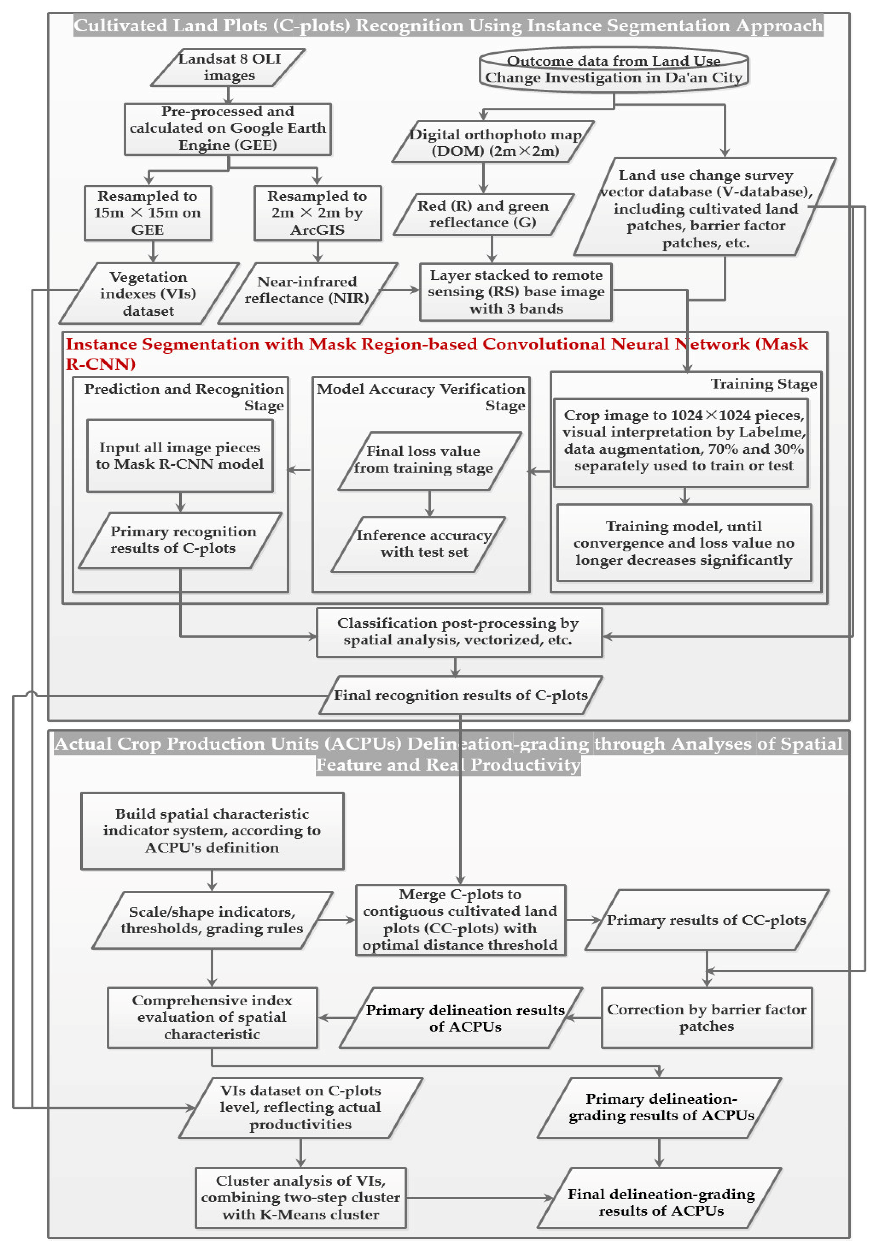
3.1.4. Identification and post-processing

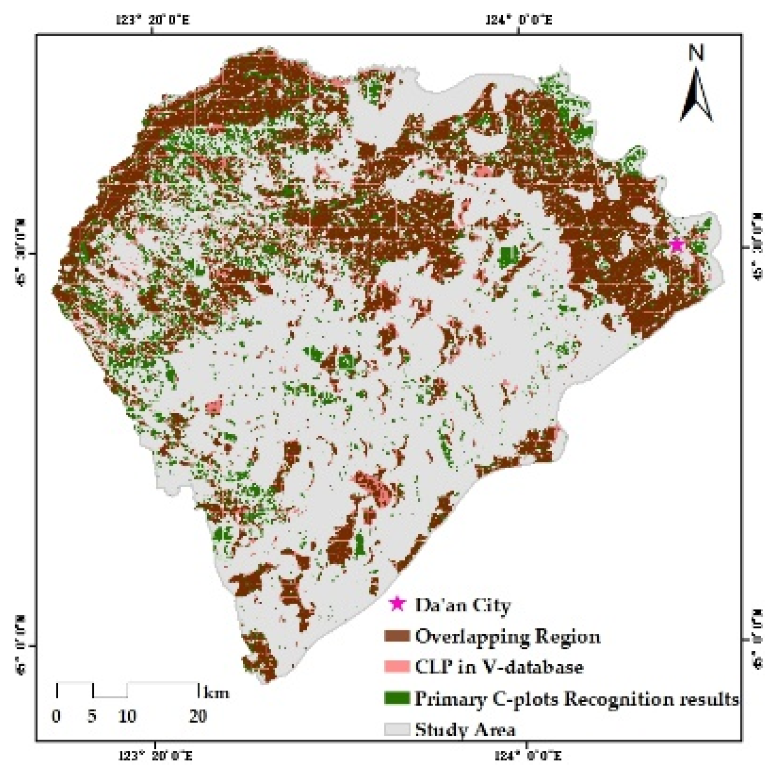
In this paper, the RS base map of the whole region (47,072 × 46,523) was separated into unified image blocks (1023 × 1011), which were put into the optimal Mask R-CNN model to receive the C-plots in every block. The recognition results of the global C-plots were comprised of the image blocks’ result graphs according to the order of the image blocks and the original size of whole base map. However, the resulting graph was superposition of the instance mask and the initial RS base map, where the values of the overlapping pixels were changed significantly and regularly. The regular differences were used in the decision tree (DT) solely to extract the instance mask. The preliminary C-plot identification results in a vector format were obtained by several types of spatial analyses such as vectorization, area screening, clip, etc.

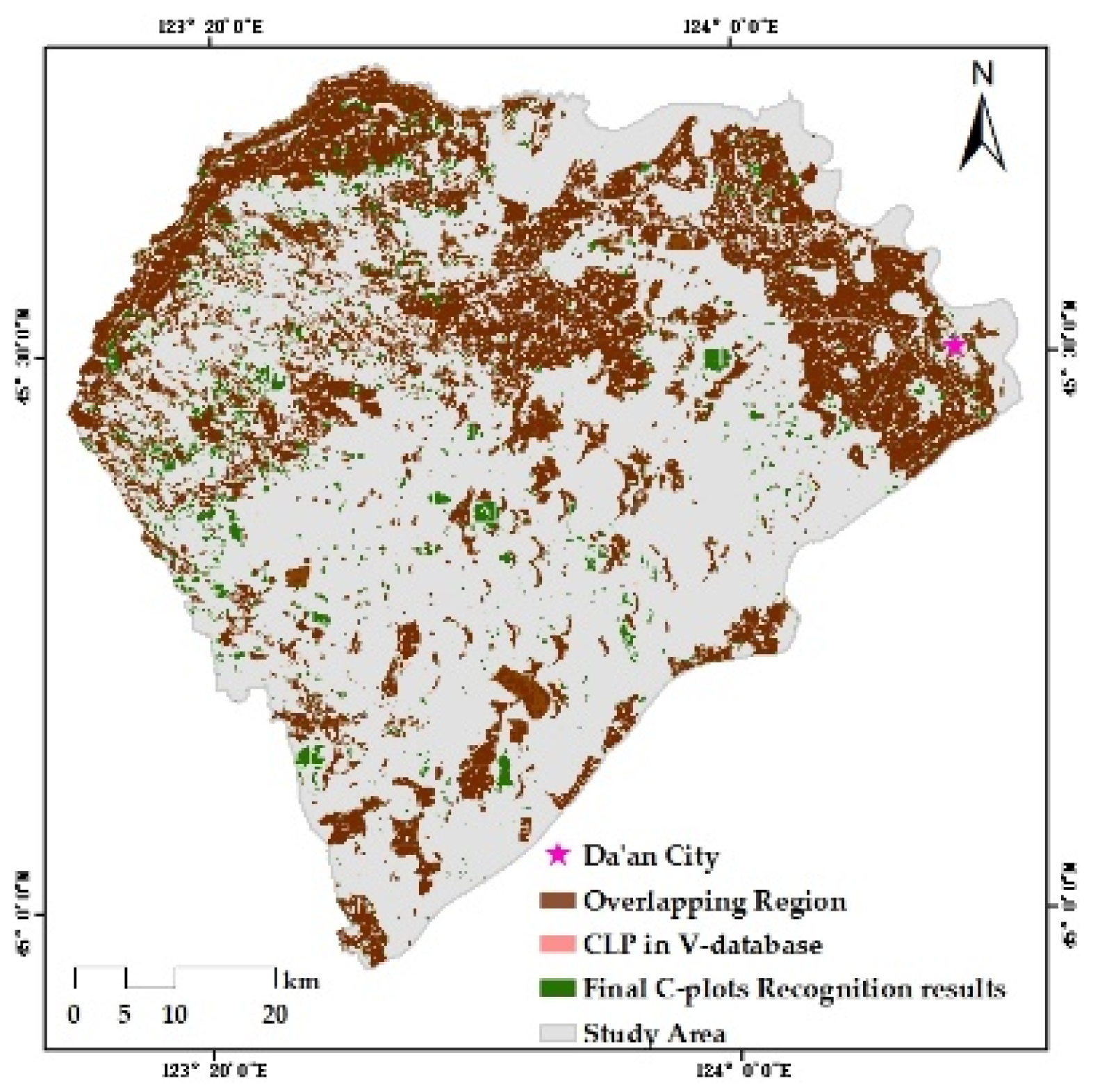
Verifying the Mask R-CNN model mainly concerns the prediction performance of the model in the target category and the group’s spatial distribution, while the ability to distinguish intra-class individuals is not fully tested. The discrimination ability of C-plot instances is further improved through post-processing. In this paper, the preliminary C-plot identification results were constrained and corrected by the V-database with authoritative auxiliary data regarded as the approximate ground truth. Specifically, the barrier factor patches of the V-database (some roads, rivers, etc.) were used for the erase operation. Cultivated land patches (CLPs) in the V-database were used to update the preliminary results and modify the instance boundaries. More detailed identification results were obtained, which are the data foundation for the delineation and grading of ACPUs.

There were three steps in the updating process: (1) the elementary recognition results were identified by CLPs to obtain the overlapping region between each CLP and C-plot instance; (2) the area ratio of every overlapping region was counted to determine the spatial fit degree between each C-plot instance and the corresponding CLP with IOU; (3) various update rules were determined by setting IOU thresholds. If IOU = 0 or 0.3 ≤ IOU < 0.6, the corresponding CLP would be preserved. If 0 < IOU < 0.3, the C-plot instance would be retained. If 0.6 ≤ IOU ≤ 1.0, the union of relevant C-plot instance and CLP would be reserved. If the C-plot instance did not overlap with any CLP, it would also be retained.

3.2. Delineation and grading of ACPU

3.2.1. Spatial characteristic indicator system

Spatial characteristics are the main evidence for the preliminary delineation and grading of ACPUs. These characteristics are usually analyzed from the perspectives of scale (area and spatial distribution) and shape, combined with the physical significance of various landscape indexes and the influence rules of the cultivated land’s spatial characteristics on agricultural production-ecology [18,58]. Considering the research scale of the ACPU, CC-plots are the units used for indicator calculation and analysis and are interpreted as a set of adjacent C-plots within a reasonable distance in a non-blocking state.

In terms of scale-area, the mean of the C-plot scale within the CC-plot (I1), the CC-plot scale (I2), and the standard deviation of the C-plot scale within the CC-plot (I3) were selected as the indicators. For the scale–spatial distribution, two indicators, including C-plot density (I4) and C-plot separation (I5), within the CC-plot were determined. In terms of shape, the mean of the C-plot shape index (I6), the standard deviation of the C-plot shape index (I7), the mean of the C-plot fractal dimension (I8), and the standard deviation of the C-plot fractal dimension (I9) within the CC-plot were comprehensively considered. Relevant formulas and explanations of the indicators are shown in

Table 3. The spatial feature indicator system and calculation principle.

Indicator (unit)	Formula	Interpretation
I1(ha)	${\mathrm{area}}_{ave}=\frac{1}{k}{\displaystyle {\displaystyle \sum }_{i=1}^k}{\mathrm{area}}_i$	${\mathrm{area}}_{ave}$: average area of C-plots in each CC-plot; ${\mathrm{area}}_i$: area of $i$th C-plot in each CC-plot; $\mathrm{k}$: number of C-plots in each CC-plot
I2(ha)	$\mathrm{al}\_\mathrm{area}={\displaystyle {\displaystyle \sum }_{i=1}^k}{\mathrm{area}}_i$	$\mathrm{al}\_\mathrm{area}$: area of each CC-plot
I3(ha)	$\mathrm{std}\_\mathrm{area}=\sqrt{\frac{1}{k}{\displaystyle {\displaystyle \sum }_{i=1}^k}{\left({\mathrm{area}}_i-{\mathrm{area}}_{ave}\right)}^2}$	$\mathrm{std}\_\mathrm{area}$: area standard deviation of C-plots in each CC-plot
I4(/ha)	$\mathrm{dens}=\frac{k}{\mathrm{al}\_\mathrm{area}}$	$\mathrm{dens}$: density of C-plots in each CC-plot
I5(/km3)	$\mathrm{sepa}=\frac{\sqrt{dens}}{2\mathrm{al}\_\mathrm{area}}$	$\mathrm{sepa}$: separation degree of C-plots in each CC-plot
I6	${\mathrm{shape}}_{ave}=\frac{1}{k}{\displaystyle {\displaystyle \sum }_{i=1}^k}(\frac{0.25p_i}{\sqrt{{\mathrm{area}}_i}})$	${\mathrm{shape}}_{ave}$: average landscape shape index of C-plots in each CC-plot; $p_i$: perimeter of $i$th C-plot in each CC-plot
I7	$\mathrm{std}\_\mathrm{shape}=\sqrt{\frac{1}{k}{\displaystyle {\displaystyle \sum }_{i=1}^k}{(\frac{0.25p_i}{\sqrt{{\mathrm{area}}_i}}-{\mathrm{shape}}_{ave})}^2}$	$\mathrm{std}\_\mathrm{shape}$: landscape shape index standard deviation of C-plots in each CC-plot
I8(/km)	${\mathrm{FRAC}}_{ave}=\frac{1}{k}{\displaystyle {\displaystyle \sum }_{i=1}^k}\left(2\ln \left(\frac{p_i}{4}\right)/\ln \left({\mathrm{area}}_i\right)\right)$	${\mathrm{FRAC}}_{ave}$: average landscape fractal dimension of C-plots in each CC-plot
I9(/km)	$\mathrm{std}\_\mathrm{FRAC}=\sqrt{\frac{1}{k}{\displaystyle {\displaystyle \sum }_{i=1}^k}{\left(2\ln \left(\frac{p_i}{4}\right)/\ln \left({\mathrm{area}}_i\right)-{\mathrm{FRAC}}_{ave}\right)}^2}$	$\mathrm{std}\_\mathrm{FRAC}$: landscape fractal dimension standard deviation of C-plots in each CC-plot

. Given the different dimensions of the indicators, normalization of the indicators was needed to simplify the analysis process and acquire indicator scores. All indicator scores were segmented into four grades (1.0, 0.8, 0.6, and 0.4). Among these scores, 0.6 was chosen as the eligibility threshold, with which the qualified level and below-qualified level of the scores were divided. For the same indicators, there are different grading criteria in different study areas according to the policy constraints and requirements, regional characteristics, etc. In this paper, a grading threshold of I1 was determined by the agro-production features of the smallholder area and the C-plot characteristics of the Chinese Northeast plain. Grading thresholds of I2 were decided by the local agro-background of land circulation and the coexistence situation of various new agro-management entities. In relevant land regulations in China [59], the shape targets of the C-plots are rectangles with a length–width ratio in a certain range; in this way, the scoring thresholds of I6 and I8 were confirmed. I4 and I5 are landscape indexes with physical meanings, whose grading thresholds were determined by the natural break point method from regional characteristics, physical meanings, and a priori knowledge. I3, I7, and I9 are the derivative indicators of related intuitive indicators that represent the relative advantages/disadvantages and consistency within a certain region. Their scoring thresholds were also determined by the natural break point method from regional characteristics and a priori knowledge.

3.2.2. Preliminary delineation and grading

The essence of an ACPU is an open agricultural system with an uncertain and fuzzy boundary [60], and the ACPUs were delineated in this paper. First, the optimal threshold of spatial distance was determined through experiments. The C-plots were fused to CC-plots. The CC-plots were cut by the barrier elements in V-database. Then, the preliminary delineation of the ACPUs was obtained. Determining a reasonable distance threshold was the key to the above processes. Wang et al. [61] considered 20 m to be the best distance threshold for cultivated land for contiguous basic farmland management in China. Therefore, 10, 20, and 30 m were selected as the distance thresholds. Three different CC-plot delineation scenarios were employed in this paper. The basis for choosing the best scheme involved quantitative constraints from the above indicators (I3, I7, and I9, etc.). The best delineation scheme had more C-plots with indicator scores no less than 0.6.

The initial delineation of the ACPUs was preliminarily evaluated and graded with the spatial feature indicator system and comprehensive index evaluation. For evaluating the scale and shape characteristics in this paper, each related indicator was considered to be of similar importance. The scale characteristic score and shape characteristic score were obtained by a weighted summation of the equal-weight assignment. Then, two kinds of characteristic scores were divided into excellent (I), qualified (II), and under-qualified (III) levels by taking 0.8 and 0.6 as the threshold values.

3.2.3. Refined delineation and grading

In the study area, local climatic conditions and soil properties decide the ripening of a single crop (one-year-one-harvest) and its planting structure mainly based on maize and rice. Thus, the annual phenophases of mainstream crops have a generally consistent trend, which ensures that we can scientifically obtain crop growth states and the actual production capacity by clustering multiple VIs. In addition, salinization is considered to be one of the most intuitive factors that affects productivity and causes spatial differentiation. The internal C-plots within the same ACPU are required to have consistent actual productivity. In the refining process of ACPUs, the productivity grading of C-plots is required. In the flourishing period of crops, the greater the VIs are, the better the growth state is, and the higher the real production capacity is. The grouping of C-plot productivities was achieved by the unsupervised cluster method, due to the complicated formation mechanism of real productivity and a lack of prior knowledge.

Common cluster algorithms include partitioning methods, hierarchical methods, density-based methods, and sliding-window-based methods. Partitioning methods are simple to calculate and suitable for a large sample size. However, the number of groups should be known beforehand, and the interference of outliers cannot be excluded. Hierarchical methods can provide rich cluster schemes without the number of groups being specified in advance. However, the applicable conditions and presuppositions are relatively strict. Each step for merging or splitting cannot be undone or changed. Density-based methods are greatly influenced by the density threshold and have unstable effects. Sliding-window-based methods do not need to know the number of groups beforehand and are less affected by mean values but are greatly affected by the radius of the sliding window. Various clustering methods have their own advantages and disadvantages but also complement each other. Therefore, a cluster method [62] combining the hierarchical method (two-step cluster) with the partitioning method (K-Means cluster) was adopted in this paper. The two-step cluster algorithm is an improved version of the balance iterative reducing and clustering using the hierarchies (BIRCH) method. The optimal group number is automatically determined. The abnormal values are deleted, thus combining the advantages of density-based methods. The specific process is divided into two stages: (1) the pre-clustering stage: the clustering feature (CF) tree is built by reading data points in turn, which is used to explore the relevant distances based on the idea of constructing the CF tree in BIRCH. Data points in the same tree node are highly similar, while points with poor similarity are used to generate new nodes. Tree nodes are sub-clusters; (2) the clustering stage: the sub-clusters are taken as objects and merged using the hierarchical agglomerative clustering (HAC) algorithm based on the distances measured by the log-likelihood function. Each cluster is judged by the Bayesian information criterion (BIC) or Akaike’s information criterion (AIC). Then a reasonable number of clusters and clustered results are obtained.

In this paper, the VIs dataset at the C-plot level was selected as the initial clustering data set. Firstly, the optimal group number was determined, and the outliers were found through a two-step cluster. Then, the interference of outliers was removed from the initial data set, and the final data set was obtained. Finally, the K-Means cluster was adopted to obtain the real productivity clustering result of each C-plot, in which the value of K was adjusted through experiments based on the optimal group number. The final delineation-grading results of the ACPUs were acquired by refining preliminary delineation-grading using groups of actual productivities.

4. Results and discussion

4.1. Identification results of C-plots through Mask R-CNN and post-processing

The optimal network parameter set (see

Table 4. Optimal network parameters for Mask R-CNN training.

Parameter	Value	Parameter	Value
GPU number	1	Total number of positive and negative anchors for RPN training	256
Input image size	3 × (1024 × 1024)	IOU threshold of NMS to filter proposals in RPN	0.9
Image number trained at once	2	ROI number output from the proposal layer for training (inference)	2000 (1000)
Iteration number in each epoch	2,000	ROI number exported from the detection target layer	200
Validation number in each epoch	50	Positive ratio of the ROI for three-branch	0.66
Backbone for feature extraction	ResNet101	Fixed size for feature maps in the ROI alignment layer	[7,7]/[14,14]
Step size of each feature layer	[4,8,16,32,64]	Size of the mask output from the mask prediction branch	[28,28]
Category	C-plot, background	Maximum number of ROIs validated per image	100
Step length of the anchor generation in RPN	1	Classification confidence of the ROIs validated	0.7
Length size of the anchor in RPN	[32,64,128,256,512]	IOU threshold of the NMS to avoid ROI or mask stacking	0.3
Horizontal–vertical ratios of the anchor in RPN	[0.5, 1, 2]	Learning rate	0.0001
Maximum ground truth instances for each image	100	Learning momentum	0.9

) was determined by comparing the training loss and inference accuracy through contrast experiments. In total, the training process lasted 16 epochs with 16 model files (.h5) saved. The model parameters were optimized based on the loss of the whole framework ($L_{all}$), using equal sums of $L_{RPN}$ (including $L_{RPN1}$ and $L_{RPN2}$) and $L_{MRCNN}$. A set of samples and the corresponding recognized results is illustrated in Figure 4.

The changes of $L_{all}$ and mAP with epoch number are shown in Figure 5. After about 6 h of training with an epoch number of 12, $L_{all}$ stopped dropping when it reached about 0.16. Therefore, the training results of the 12th epoch were selected as the prediction model to preliminarily identify global C-plot instances (see Figure 6) with an inference accuracy of 82.29%. This offered a superior matched degree to the reality for the area and the overall distribution of recognized C-plots. However, the separating capacity of the model between the instances in the C-plot group was not proven. The quantity-space matched degree between the initial identification results and the reality is shown in

Table 5. Statistical comparison of the recognition results with the approximate ground truth.

	Dataset	Ground Truth	Preliminary Results	Post-Processing Results
Comparison Item
Area of cultivated land (ha)		139,050.60	163,811.71	157,911.17
Quantity match area ratio		--	82.19%	86.44%
Space overlap area ratio		--	79.11%	100%
Number of C-plots		20,680	3344	37,726
Diff-number of C-plots		--	-17,336	+17,046

: (1) the quantity difference was relatively small when comparing the C-plot area with the total cultivated area of the approximate ground truth. (2) The space–overlap ratio was comparatively large when contrasting the distribution of C-plots with the real cultivated land. The revised results are shown in Figure 7 after spatial analysis and post-processing based on auxiliary data. The differences of the C-plot numbers between the recognition results and the ground truth are shown in Table 5: (1) before post-processing, the primary recognition results were 17,336 fewer than the ground truth. The C-plot instances from Mask R-CNN were rougher than the actual situation. It was common for many pieces of cultivated land to be misidentified to the same C-plot instance, likely because of the RS base image’s resolution limitations. (2) After post-processing, the quantity and space-matched degree were both improved. The C-plot number for final recognition results obviously exceeded the ground truth, while the area was closer to the ground truth. In this way, the instance boundaries of the C-plots were refined, and the individual-level discrimination accuracy of the C-plot group was improved.

4.2. Preliminary delineation of ACPU

The delineation plans for the CC-plots were obtained by the distance threshold values of 10, 20, and 30 m. The statistical results of I3, I7, and I9 are shown in

Table 6. Statistical comparison of the CC-plot delineation plans.

Distance Threshold (m)	10	20	30
Number of CC-plots	4136	3305	2719
Number of reasonable CC-plots 2	3922	3139	2585
Number ratio of reasonable CC-plots	94.83%	94.98%	95.07%
Area of CC-plots	157,911.17
Area of reasonable CC-plots	133,274.96	151,116.35	154,082.92
Area ratio of reasonable CC-plots	84.40%	95.70%	97.58%

² Reasonable CC-plots refer to CC-plots with scores of I3, I7, and I9 higher than 0.6.

: (1) plans using 20/30 m were much better than that using 10 m based on the ratio of reasonable CC-plots. (2) The proportion difference between the plans using 20 and 30 m was small, but the threshold of 30 m was significantly more likely to form production barriers than 20 m. Thus, 20 m was ultimately determined as the most reasonable distance threshold to delineate the CC-plots, considering previous studies [61]. In total, 3305 initial ACPUs were obtained after erasing the block elements.

4.3. Preliminary grading of ACPUs through spatial characteristic analysis

Grades of the scale and shape features are shown in Figure 8 based on the initial ACPUs, the aforementioned spatial characteristic indicator system, grading rules, and a comprehensive index evaluation: (1) the scale feature scores of the initial ACPUs were [0.52, 1.00], with little spatial differentiation. The average score was 0.76. Grade I accounted for a large proportion, while there were a small proportion and a dispersed distribution in the lower grades. Thus, the scale of most initial ACPUs was reasonable. The higher grades mainly corresponded to the area with dense cultivated land, while the lower grades corresponded to the area with scattered and fragmented cultivated land. This result is in line with local agricultural reality. (2) The shape feature scores were [0.45, 1.00] with an average of 0.84. The cultivated land mainly belonged to Grade II, while areas of Grade I or III were relatively small. The higher grades were mostly concentrated in the northwest, central, and eastern regions; meanwhile, the lower grades were largely distributed in the north central, and northeast areas. Most of the initial ACPUs featured reasonable shape characteristics (Grade I or II), and others featured less qualified shapes corresponding to regions with shape-complicated cultivated land. (3) For the initial ACPUs, higher scale feature scores were usually associated with better shape features and vice versa. The superimposed grading results of the spatial features are also shown in Figure 8: (1) a total of eight combination grades were formed: I-I, I-II, I-III, II-I, II-II, II-III, III-I, and III-II. (2) The combined grading results featured strong spatial consistency with their shape features while the spatial differences of the scale features were very small, which indicates that their shape was better than their scale in determining spatial feature grading.

4.4. Refined results of ACPU across productivity cluster

The two-step cluster results (see Figure 9) were illustrated, showing that (1) the cluster quality was good with an optimal cluster number of 3. The proportions of all clusters were within an acceptable range. The differentiation degree of variables among the clusters was high. (2) A total of 994 outliers were found and identified, while the mean values of all variables were significantly lower than the non-outliers

In total, 994 outliers were extracted from the original objects to a separate cluster named Outlier, while the K-Means cluster was used for the rest of the original objects. In reference to the optimal cluster number from the two-step cluster, K-values of 2, 3, and 4 were applied to the test (see

Table 7. Statistical comparison of K-Means cluster plans.

K	Cluster ID (Number Ratio)	Statistics Value	VCI	TVI	RVI	NDVI	GNDVI
2	1 (44.48%)	Mean	80.09	1.05	4.49	0.60	0.60
		Std.	1.53	0.01	0.47	0.03	0.02
	2 (55.52%)	Mean	75.36	1.00	3.38	0.51	0.53
		Std.	2.49	0.03	0.44	0.05	0.04
3	1 (13.04%)	Mean	82.22	1.07	5.14	0.64	0.63
		Std.	1.05	0.01	0.32	0.02	0.02
	2 (21.23%)	Mean	72.89	0.98	2.94	0.46	0.49
		Std.	2.38	0.03	0.35	0.05	0.04
	3 (65.73%)	Mean	78.00	1.03	3.92	0.56	0.57
		Std.	1.29	0.01	0.32	0.03	0.02
4	1 (10.53%)	Mean	82.60	1.07	5.25	0.65	0.64
		Std.	0.75	0.01	0.24	0.01	0.01
	2 (12.99%)	Mean	71.57	.96	2.74	0.43	0.47
		Std.	2.17	0.02	0.31	0.04	0.04
	3 (43.45%)	Mean	76.55	1.01	3.59	0.53	0.55
		Std.	0.99	0.01	0.24	0.02	0.02
	4 (33.03%)	Mean	79.34	1.04	4.27	0.59	0.59
		Std.	0.54	0.01	0.17	0.01	0.01
Overall		Mean	77.46	1.02	3.88	0.55	0.56
		Std.	3.16	0.03	0.71	0.06	0.05

): (1) each of the three clustering results ensured greater inter-cluster differences, smaller intra-cluster variances, and obvious differences with the Cluster Outlier. (2) The distribution of the cluster size was unreasonable when K was set to 3 because the size of Cluster 3 was significantly larger than that of the others. (3) The results with K = 4 were relatively more detailed and reasonable than those with K = 2 due to refining inter-cluster differences and keeping intra-cluster variances. Therefore, the real productivities of the global C-plots were divided into five clusters—four from K-Means and one Outlier. There was a uniform relative relationship among the variables’ mean values for the five clusters in descending order: Cluster 1 > 4 > 3 > 2 > Outlier. Cluster 1 corresponded to superior (Grade I) productivity. Cluster 4 was consistent with good (Grade II) productivity. Cluster 3 coincided with medium (Grade III) productivity. Cluster 2 agreed with low (Grade IV) productivity. The Outlier cluster corresponded to poor (Grade V) productivity. Details are shown in Figure 10: the productivities at all grades involved a certain spatial aggregation. Notably, Grades I–III were mainly distributed in areas with the concentrated contiguous cultivated land. Here, the benefits of large-scale agro-production and the spatial distribution law of the natural background are reflected.

After refining using productivity grades, the final delineation-grading results of the ACPUs were obtained (as shown in Figure 11). In the whole region, a total of 3314 ACPUs were obtained, and eight spatial feature grades were superimposed with five productivity levels to form 38 combined grades. According to the distribution acreage, the final combined grades of the ACPUs in the study area were dominated by I-II-II, I-II-III, I-II-I, I-II-III, I-II-III, I-II-IV, I-I-IV, I-I-II, and I-II-V (Figure 12), while other grades featured limited distribution. Grade I-II-II, Grade I-II-III, and Grade I-II-I occupied most of the ACPUs in the central, eastern, and northwestern areas, covering the main distribution area of the local cultivated land. Therefore, there were reasonable scale-shapes for most of the ACPUs, which met the needs of large-scale, mechanized production and ensuring a productivity of medium or above. A statistical chart comparing spatial characteristic grades with productivity grades is provided in Figure 13: (1) Grade I-II, for spatial features, covered much of the area in each grade of productivities, especially in Grade II. (2) Grade I-I, for spatial features, was mainly distributed in Grade I and II for productivity. (3) Grade I-III for spatial feature was mostly deposited in Grade III for productivity. The spatial characteristics of ACPUs were not completely consistent with the distribution of productivities. Productivities were not only influenced by spatial features but also by regional natural resource distribution, farming management, etc. In actual agro-production, productivity can be improved by adjusting spatial features or farming management using natural resources as the basis. In addition, farming management is also heavily influenced by spatial characteristics.

4.5. Discussion

Production information acquisition is significant to achieve agricultural supervision and guidance in modern smallholder areas. The delineation and grading of production units are the basis for obtaining such production information. However, most of the existing studies are about the overall extraction and evaluation of the crop area, not the production units in modern smallholder areas based on multi-source/multi-scale RS images and ML. Thus, in this paper, a combined delineation-grading method for ACPUs in modern smallholder areas was proposed on the basis of RS images, Mask R-CNN, spatial analysis, comprehensive index evaluation, and cluster analysis. Da’an City features abundant agricultural water-soil resources. The benign coexistence of various agro-subjects has been achieved in recent years through land transfer and other measures [17]. The agricultural production units are representative and feature typical modern smallholder characteristics. Therefore, there are reference values for similar modern smallholder regions based on the research methods and results of this paper.

Firstly, the ACPU concept was presented using modern smallholder features with a scale between traditional agricultural C-plots and modern crop areas. The definition rules for ACPUs mainly consider the consistency of output and production modes, which are different from the production resource allocation considered by previous farming units. The advantages include the following: (1) the delineation results were more objective when the real outputs were taken as the reference standards. (2) Various production resources have different service modes and scopes in the work process, so delineating production units is very difficult using previous definition rules, whose validation tests are also difficult.

Secondly, a C-plot identification method was proposed to assist ACPU delineation, which is suitable for modern smallholder areas based on high-resolution RS images and Mask R-CNN. In recent years, the accuracy of crop area recognition, classification, and mapping has improved. In particular, significant results have been presented with the development of RS and ML technology. Originally, the main crop classification accuracy could reach about 85% [14] by combining multilevel DL architecture based on multi-temporal medium-resolution RS and SAR with geographical spatial data post-processing. Subsequently, the incorporation of time series data from medium-resolution RS (MODIS, Landsat, GF1, etc.) and various CNNs brought the accuracy up to 85.54% [11]. Recently, the effectiveness and superiority of using more DL algorithms in crop area extraction based on multi-temporal SAR or high-resolution optical images has been proven [8,9,10,12,13,15]. Some studies have made efforts in smallholder farming areas. The relevant accuracies can reach 85% [6] or even 95% [7] by using an improved FCN or a variety of deep semantic segmentation networks with multi-temporal SAR or sub-meter resolution RS images. Referring to Section 4.1, the method proposed in this paper was evaluated in the following ways: (1) instance segmentation was used to recognize C-plots for the first time. Instance segmentation was mainly used to solve the classification problems of natural close shot images, while RS images are much different in their responses to the effects of resolution, target diversity, and the relative size of target and view field. (2) For the recognition results, the overall regional distribution at the pixel level have focused on common algorithms (semantic segmentation, etc.), while individual C-plots and the boundaries of C-plots at the object level were emphasized in this paper. (3) The evaluation units of existing studies are usually random sample points, and the evaluation results are only related to a single pixel. In this paper, the object-level instance boxes were the assessment units. The estimation results were related to all pixels in the whole box and the IOU threshold. Thus, the latter approach is more stringent than the former. In conclusion, there is no absolute but rather relative comparability between existing methods and the presented method in this paper. Furthermore, mAP reached more than 82%, so the presented method is considered to be an effective attempt to provide relatively reliable C-plots for modern smallholder regions.

Thirdly, comparing the initial C-plots from instance segmentation with the CLPs from V-database, the area and spatial overlaps were well matched, respectively, with 82.19% and 79.11%: (1) the CLPs in V-database were obtained from RS images with a sub-meter resolution, while the C-plots used a 2 m resolution. These two kinds of images are inherently different in several ways, such as boundary detail, richness, and separability, especially in areas with dense C-plots. Therefore, a number of adjacent C-plots were roughly segmented into one instance for the preliminary identification results of the C-plots. The boundaries of the C-plots were likely refined, and the matching degree of each individual number was likely increased when the RS images’ spatial resolutions were improved to a sub-meter level. (2) The area and spatial overlaps were significantly enhanced. The individual boundaries of the C-plots were refined to increase the discrimination accuracy at instance level in the densely distributed area of cultivated land based on the auxiliary data and spatial analysis.

Fourth, the delineation basis for ACPUs was the CC-plot designation according to specific rules: (1) a reasonable spatial threshold for judging whether the C-plots are contiguous under their scale characteristics for modern smallholder production; (2) the distribution of barrier elements in production, which is emphasized by landscape ecology [63]; (3) the required shape and scale consistency for internal C-plots in the ACPU concept. Based on previous studies [61] and the actual situation of the research area, 10, 20, and 30 m were taken as the distance thresholds of the CC-plots to determine the best option. Meanwhile, the blocking effects of the barrier elements in production were mainly achieved by a spatial analysis based on data from V-database. The shape and scale consistency of the C-plots within the CC-plots were achieved by calculating the spatial characteristic indicators’ standard deviation, with which the rationality of the CC-plots was quantitatively described. The basis for selecting the best distance threshold was also provided. The final CC-plots were regarded as the initial ACPUs, which were more objective than those in existing studies. Moreover, a spatial characteristic indicator system was constructed for preliminary ACPU grading, while multiple VIs in the crop flourishing period were calculated to cluster the C-plots’ productivities to refine the initial delineation-grading results of the ACPUs.

The method of ACPU delineation-grading was applied to Da’an City. The results agree with local reality. However, there are still some problems that need further study: (1) for C-plot instance segmentation, the boundaries of the C-plots were coarse due to the limitations of the resolution of the RS base map. (2) For the RS images, only three characteristic bands were used for instance segmentation with limited feature information. The accuracy of the recognition results will likely be improved if multi-temporal and multi-feature data with more useful information are adopted. (3) The grade thresholds of the part indicators in the spatial characteristic indicator system need to be uniformly defined. Determination based on the natural break point method and prior knowledge may lead to irrationality.

5. Conclusions

The acquisition and evaluation of production units are an important basis for agricultural production and management in modern smallholder regions. In this paper, a method of delimitation-grading for agro-production units in modern smallholder regions was explored. Some conclusions can be drawn:

(1) The ACPU is interpreted reasonably from the perspectives of production mode, spatial form, and productivity, combining regulatory needs with production results.

(2) An effective method for C-plot instance recognition is provided by using Mask R-CNN and high-resolution RS images. The loss of the best model is about 0.16, with the mAP at about 82.29%. The recognition accuracy of the C-plots is significantly improved by combining traditional methods (spatial analysis, etc.) with the instance segmentation algorithm. The area–space overlap and fine degree of C-plots are improved noticeably after the modification of auxiliary data.

(3) The reasonable designation of CC-plots is the basis for ACPU delineation-grading; 20 m is the most reasonable distance threshold for CC-plots. The preliminary grading of ACPUs can be achieved by a comprehensive index evaluation. The spatial feature indicator system of the comprehensive index evaluation is constructed from the two dimensions of scale and shape, including nine specific indicators that involve multiple landscape indexes and standard deviations.

(4) The VIs are used to characterize the C-plots’ actual productivities by combining two-step cluster and K-Means. The global C-plots’ productivities are divided into five grades with clear physical significances, through which the ACPUs’ delineation-grading results were reasonably refined.

(5) Most of the ACPUs in the study area have a reasonable scale and appropriate shape, demonstrating medium or above actual productivities. These ACPUs are suitable for large-scale mechanized production for modern smallholders. However, the spatial characteristics of ACPUs are not completely consistent with their productivities. Natural resources are taken as the basis to improve productivity by adjusting the ACPUs’ spatial characteristics, farming management, etc.

The delimitation-grading method for the ACPUs proposed in this paper is flexible and can be adjusted according to the changes in the study areas with strong extensibility to provide a reference for the supervision of agro-production in many modern smallholder areas.

References

1. Brundtland, G.H.; Khalid, M.; Agnelli, S.; Al-Athel, S. Our Common Future; World Commission on Environment and Development: New York, NY, USA, 1987. [Google Scholar]
2. United Nations. United Nations Sustainable Development Goals. In Proceedings of the United Nations Conference on Sustainable Development, Rio de Janeiro, Brazil, 20–22 June 2012.
3. Brown, M.E.; De Beurs, K.M.; Marshall, M. Global phenological response to climate change in crop areas using satellite remote sensing of vegetation, humidity and temperature over 26 years. Remote Sens. Environ. 2012, 126, 174–183. [Google Scholar] [CrossRef]
4. Kuenzer, C.; Knauer, K. Remote sensing of rice crop areas. Int. J. Remote Sens. 2013, 34, 2101–2139. [Google Scholar] [CrossRef]
5. Lv, Y.; Zhang, C.; Ma, J.; Yun, W.; Gao, L.; Li, P. Sustainability Assessment of Smallholder Farmland Systems: Healthy Farmland System Assessment Framework. Sustainability 2019, 11, 4525. [Google Scholar] [CrossRef] [Green Version]
6. Wei, S.; Zhang, H.; Wang, C.; Wang, Y.; Xu, L. Multi-temporal SAR data large-scale crop mapping based on U-Net model. Remote Sens. 2019, 11, 68. [Google Scholar] [CrossRef] [Green Version]
7. Du, Z.; Yang, J.; Ou, C.; Zhang, T. Smallholder Crop Area Mapped with a Semantic Segmentation Deep Learning Method. Remote Sens. 2019, 11, 888. [Google Scholar] [CrossRef] [Green Version]
8. Cué La Rosa, L.E.; Queiroz Feitosa, R.; Nigri Happ, P.; Del’Arco Sanches, I.; Ostwald Pedro da Costa, G.A. Combining Deep Learning and Prior Knowledge for Crop Mapping in Tropical Regions from Multitemporal SAR Image Sequences. Remote Sens. 2019, 11, 2029. [Google Scholar] [CrossRef] [Green Version]
9. Zhou, Y.; Luo, J.; Feng, L.; Zhou, X. DCN-Based Spatial Features for Improving Parcel-Based Crop Classification Using High-Resolution Optical Images and Multi-Temporal SAR Data. Remote Sens. 2019, 11, 1619. [Google Scholar]
10. Zhao, H.; Chen, Z.; Jiang, H.; Jing, W.; Sun, L.; Feng, M. Evaluation of Three Deep Learning Models for Early Crop Classification Using Sentinel-1A Imagery Time Series—A Case Study in Zhanjiang, China. Remote Sens. 2019, 11, 2673. [Google Scholar] [CrossRef] [Green Version]
11. Zhong, L.; Hu, L.; Zhou, H. Deep learning based multi-temporal crop classification. Remote Sens. Environ. 2019, 221, 430–443. [Google Scholar] [CrossRef]
12. La Rosa, L.E.C.; Happ, P.N.; Feitosa, R.Q. Dense Fully Convolutional Networks for Crop Recognition from Multitemporal SAR Image Sequences. In Proceedings of the 2018 IEEE International Geoscience and Remote Sensing Symposium, Valencia, Spain, 22–27 July 2018; pp. 7460–7463. [Google Scholar]
13. Ji, S.; Zhang, C.; Xu, A.; Shi, Y.; Duan, Y. 3D Convolutional Neural Networks for Crop Classification with Multi-Temporal Remote Sensing Images. Remote Sens. 2018, 10, 75. [Google Scholar] [CrossRef] [Green Version]
14. Kussul, N.; Lavreniuk, M.; Skakun, S.; Shelestov, A. Deep learning classification of land cover and crop types using remote sensing data. IEEE Geosci. Remote Sens. Lett. 2017, 14, 778–782. [Google Scholar] [CrossRef]
15. Castro, J.D.B.; Feitoza, Q.; La Rosa, L.C.; Achanccaray Diaz, P.M.; Arco Sanches, I.D. A Comparative analysis of deep learning techniques for sub-tropical crop types recognition from multitemporal optical/SAR image sequences. In Proceedings of the 2017 30th SIBGRAPI Conference on Graphics, Patterns and Images (SIBGRAPI), Niteroi, Brazil, 17–20 October 2017; pp. 382–389. [Google Scholar]
16. Kuwata, K.; Shibasaki, R. Estimating crop yields with deep learning and remotely sensed data. In Proceedings of the 2015 IEEE International Geoscience and Remote Sensing Symposium (IGARSS), Milan, Italy, 26–31 July 2015; pp. 2015–2858. [Google Scholar]
17. Liu, Z. Current situation analysis of land circulation in Da’an City. Agric. Jilin 2014, 10, 60. [Google Scholar]
18. Lv, Z.; Hao, J.; Niu, L. Study on the plots’ geometrical feature and its effects on the mechanized farming in Huang-Huai-Hai plain: An empirical study of Quzhou County in Hebei Province. J. China Agric. Univ. 2016, 21, 97–103. [Google Scholar]
19. Li, X.; Dong, X.; Xu, Y. study on the evolution characteristics and influencing factors of faming unit in china. Chin. J. Agric. Resour. Reg. Plan. 2016, 5, 20–26. [Google Scholar]
20. Li, Y.; Qi, H.; Dai, J.; Ji, X.; Wei, Y. Fully convolutional instance-aware semantic segmentation. In Proceedings of the IEEE Conference on Computer Vision and Pattern Recognition, Honolulu, HI, USA, 21–26 July 2017; pp. 2017–2359. [Google Scholar]
21. He, K.; Gkioxari, G.; Dollár, P.; Girshick, R. Mask r-cnn. In Proceedings of the IEEE International Conference on Computer Vision, Venice, Italy, 22–29 October 2017; pp. 2017–2961. [Google Scholar]
22. Liu, S.; Qi, L.; Qin, H.; Shi, J.; Jia, J. Path aggregation network for instance segmentation. In Proceedings of the IEEE Conference on Computer Vision and Pattern Recognition, Salt Lake City, UT, USA, 18–23 June 2018; pp. 2018–8759. [Google Scholar]
23. Hu, R.; Dollár, P.; He, K.; Darrell, T.; Girshick, R. Learning to segment everything. In Proceedings of the IEEE Conference on Computer Vision and Pattern Recognition, Salt Lake City, UT, USA, 18–23 June 2018; pp. 2018–4233. [Google Scholar]
24. Chen, K.; Pang, J.; Wang, J.; Xiong, Y.; Li, X.; Sun, S.; Feng, W.; Liu, Z.; Shi, J.; Ouyang, W.; et al. Hybrid task cascade for instance segmentation. In Proceedings of the IEEE Conference on Computer Vision and Pattern Recognition, Long Beach, CA, USA, 16–20 June 2019; pp. 2019–4974. [Google Scholar]
25. Hsu, K.J.; Lin, Y.Y.; Chuang, Y.Y. DeepCO3: Deep Instance Co-Segmentation by Co-Peak Search and Co-Saliency Detection. In Proceedings of the IEEE Conference on Computer Vision and Pattern Recognition, Long Beach, CA, USA, 16–20 June 2019; pp. 2019–8846. [Google Scholar]
26. Qiao, Y.; Truman, M.; Sukkarieh, S. Cattle segmentation and contour extraction based on Mask R-CNN for precision livestock farming. Comput. Electron. Agric. 2019, 165, 104958. [Google Scholar] [CrossRef]
27. Li, D.; Zhang, K.; Li, X.; Chen, Y.; Li, Z.; Pu, D. Mounting Behavior Recognition for Pigs Based on Mask R-CNN. Trans. Chin. Soc. Agric. Mach. 2019, 4942. [Google Scholar] [CrossRef] [Green Version]
28. Yu, Y.; Zhang, K.; Yang, L.; Zhang, D. Fruit detection for strawberry harvesting robot in non-structural environment based on Mask-RCNN. Comput. Electron. Agric. 2019, 163, 104846. [Google Scholar] [CrossRef]
29. Lin, X.; Zhu, S.; Zhang, J.; Liu, D. Rice Planthopper Image Classification Method Based on Transfer Learning and Mask R-CNN. Trans. Chin. Soc. Agric. Mach. 2019, 50, 201–207. [Google Scholar]
30. Stewart, E.L.; Wiesner-Hanks, T.; Kaczmar, N.; DeChant, C.; Wu, H.; Lipson, H.; Nelson, R.J.; Gore, M.A. Quantitative Phenotyping of Northern Leaf Blight in UAV Images Using Deep Learning. Remote Sens. 2019, 11, 2209. [Google Scholar] [CrossRef] [Green Version]
31. Lu, J.Y.; Chang, C.L.; Kuo, Y.F. Monitoring Growth Rate of Lettuce Using Deep Convolutional Neural Networks. In Proceedings of the 2019 ASABE Annual International Meeting, Boston, MA, USA, 7–10 July 2019. [Google Scholar]
32. Li, D.; Chen, Y.; Zhang, K.; Li, Z. Mounting Behaviour Recognition for Pigs Based on Deep Learning. Sensors 2019, 19, 4924. [Google Scholar] [CrossRef] [Green Version]
33. Wang, X.; Wang, M.; Wang, Z. Analysis on the Influence of Climate Resources on Agricultural Production in Da’an City. Public Commun. Sci. Technol. 2013, 18, 103. [Google Scholar]
34. Liu, Y.; Yue, H.; Du, G. Analysis on the Effect of Farmland Protection and Quality Improvement in Da’an City. Agric. Technol. Serv. 2016, 18, 104. [Google Scholar]
35. Van Leeuwen, W.J.; Hartfield, K.; Miranda, M.; Meza, F.J. Trends and ENSO/AAO Driven Variability in NDVI Derived Productivity and Phenology alongside the Andes Mountains. Remote Sens. 2013, 5, 1177–1203. [Google Scholar] [CrossRef] [Green Version]
36. Abou Ali, H.; Delparte, D.; Griffel, L.M. From Pixel to Yield: Forecasting Potato Productivity in Lebanon and Idaho. Int. Arch. Photogramm. Remote Sens. Spat. Inf. Sci. 2020, 42, 1–7. [Google Scholar] [CrossRef] [Green Version]
37. Balasundram, S.K.; Memarian, H.; Khosla, R. Estimating oil palm yields using vegetation indices derived from Quickbird. Life Sci. J. 2013, 10, 851–860. [Google Scholar]
38. Rouse, J.W.; Haas, R.H.; Schell, J.A.; Deering, D.W. Monitoring Vegetation Systems in the Great Plains with ERTS; NASA Special Publication; NASA: Washington, DC, USA, 1974; Volume 351, pp. 309–317.
39. Kogan, F.; Gitelson, A.; Zakarin, E.; Spivak, L.; Lebed, L. AVHRR-based spectral vegetation index for quantitative assessment of vegetation state and productivity. Photogramm. Eng. Remote Sens. 2003, 69, 899–906. [Google Scholar] [CrossRef]
40. Tsai, Y.H.; Stow, D.; Chen, H.L.; Lewison, R.; An, L.; Shi, L. Mapping Vegetation and Land Use Types in Fanjingshan National Nature Reserve Using Google Earth Engine. Remote Sens. 2018, 10, 927. [Google Scholar] [CrossRef] [Green Version]
41. Jin, Z.; Azzari, G.; You, C.; Tommaso, S.D.; Aston, S.; Burke, M.; Lobell, D.B. Smallholder maize area and yield mapping at national scales with Google Earth Engine. Remote Sens. Environ. 2019, 228, 115–128. [Google Scholar] [CrossRef]
42. Shelestov, A.; Lavreniuk, M.; Kussul, N.; Novikov, A.; Skakun, S. Exploring Google earth engine platform for large data processing: Classification of multi-temporal satellite imagery for crop mapping. Front. Earth Sci. 2017, 5, 17. [Google Scholar] [CrossRef] [Green Version]
43. Farda, N.M. Multi-temporal land use mapping of coastal wetlands area using machine learning in Google earth engine. IOP Conf. Ser. Earth Environ. Sci. 2017, 98. [Google Scholar] [CrossRef]
44. Dong, J.; Xiao, X.; Menarguez, M.A.; Zhang, G.; Qin, Y.; Thau, D.; Biradar, C.; Moore, B., III. Mapping paddy rice planting area in northeastern Asia with Landsat 8 images, phenology-based algorithm and Google Earth Engine. Remote Sens. Environ. 2016, 185, 142–154. [Google Scholar] [CrossRef] [PubMed] [Green Version]
45. Lv, Y.; Yun, W.; Zhang, C.; Zhu, D.; Yang, J.; Chen, Y. Multi-characteristic comprehensive recognition of well-facilitied farmland based on TOPSIS and BP neural network. Trans. Chin. Soc. Agric. Mach. 2018, 49, 196–204. [Google Scholar]
46. Xu, W.; Jin, J.; Jin, X.; Xiao, Y.; Ren, J.; Liu, J.; Sun, R.; Zhou, Y. Analysis of Changes and Potential Characteristics of Cultivated Land Productivity Based on MODIS EVI: A Case Study of Jiangsu Province, China. Remote Sens. 2019, 11, 2041. [Google Scholar] [CrossRef] [Green Version]
47. Ma, J.; Zhang, C.; Yun, W.; Lv, Y.; Chen, W.; Zhu, D. The Temporal Analysis of Regional Cultivated Land Productivity with GPP Based on 2000–2018 MODIS Data. Sustainability 2020, 12, 411. [Google Scholar] [CrossRef] [Green Version]
48. Ren, S.; He, K.; Girshick, R.; Sun, J. Faster r-cnn: Towards real-time object detection with region proposal networks. In Proceedings of the Advances in Neural Information Processing Systems, Montreal, QC, Canada, 7–12 December 2015; pp. 91–99. [Google Scholar]
49. Jin, S.; Su, Y.; Gao, S.; Wu, F.; Hu, T.; Liu, J.; Li, W.; Wang, D.; Chen, S.; Jiang, Y.; et al. Deep learning: Individual maize segmentation from terrestrial lidar data using faster R-CNN and regional growth algorithms. Front. Plant Sci. 2018, 9, 866. [Google Scholar] [CrossRef]
50. Girshick, R. Fast r-cnn. In Proceedings of the IEEE International Conference on Computer Vision, Santiago, Chile, 7–13 December 2015; pp. 1440–1448. [Google Scholar]
51. Girshick, R.; Donahue, J.; Darrell, T.; Malik, J. Rich feature hierarchies for accurate object detection and semantic segmentation. In Proceedings of the IEEE Conference on Computer Vision and Pattern Recognition, Columbus, OH, USA, 24–27 June 2014; pp. 580–587. [Google Scholar]
52. He, K.; Zhang, X.; Ren, S.; Sun, J. Deep residual learning for image recognition. In Proceedings of the IEEE Conference on Computer Vision and Pattern Recognition, Las Vegas, NV, USA, 26 June–1 July 2016; pp. 770–778. [Google Scholar]
53. Lin, T.Y.; Dollár, P.; Girshick, R.; He, K.; Hariharan, B.; Belongie, S. Feature pyramid networks for object detection. In Proceedings of the IEEE Conference on Computer Vision and Pattern Recognition, Honolulu, HI, USA, 21–26 July 2017; pp. 2017–2117. [Google Scholar]
54. Ng, W.; Minasny, B.; Montazerolghaem, M.; Padarian, J.; Ferguson, R.; Bailey, S.; McBratney, A.B. Convolutional neural network for simultaneous prediction of several soil properties using visible/near-infrared, mid-infrared, and their combined spectra. Geoderma 2019, 352, 251–267. [Google Scholar] [CrossRef]
55. Ding, J.; Chen, B.; Liu, H.; Huang, M. Convolutional neural network with data augmentation for SAR target recognition. IEEE Geosci. Remote Sens. Lett. 2016, 13, 364–368. [Google Scholar] [CrossRef]
56. Maxwell, A.E.; Pourmohammadi, P.; Poyner, J.D. Mapping the Topographic Features of Mining-Related Valley Fills Using Mask R-CNN Deep Learning and Digital Elevation Data. Remote Sens. 2020, 12, 547. [Google Scholar] [CrossRef] [Green Version]
57. Lin, T.Y.; Maire, M.; Belongie, S.; Bourdev, L.; Girshick, R.; Hays, J.; Perona, P.; Ramanan, D.; Zitnick, C.L.; Dollár, P. Microsoft COCO: Common Objects in Context. Available online: https://arxiv.org/abs/1405.0312 (accessed on 15 October 2019).
58. Liu, Y.; Lliu, Q.; TANG, X.; REN, Y.; Sun, C.; Tang, L. Effects of Fragmentation of Cultivated Land Unit on Mechanical Harvesting Efficiency of Wheat in Plain Area. Trans. Chin. Soc. Agric. Mach. 2018, 49, 225–231. [Google Scholar]
59. Ministry of Natural Resources of the People’s Republic of China. Rules of Well-Facilitied Farmland Construction (GB/T30600); MNR: Beijing, China, 2014. (In Chinese) [Google Scholar]
60. Pengshan, L. Integrated Ecological Assessment of Farmland System and Trade-Offs Analysis of Functions; China Agricultural University: Beijing, China, 2017. [Google Scholar]
61. Wang, C.; Sang, L.; Yang, J.; Zhang, C.; Zhu, D.; Ming, D. Spatial Identification of Connected Arable Lands Using Geometric Network Model. Sens. Lett. 2012, 10, 341–348. [Google Scholar] [CrossRef]
62. Liu, Y.; Wu, S.; Zhou, H.; Wu, X.; Han, L. Research on optimization method based on K-means clustering algorithm. Inf. Technol. 2019, 43, 74–78. [Google Scholar]
63. Li, S. The Geography of Ecosystem Services; Science Press: Beijing, China, 2014. [Google Scholar]
Figure 1. Study area. (a) Location of Da’an City; (b) distribution of cultivated land in Da’an City; (c) distribution of soil subtypes in Da’an City; (d) distribution of landscape types in Da’an City.
Remotesensing 12 01074 g001
Figure 2. Technical flowchart.
Remotesensing 12 01074 g002
Figure 3. Architecture of the mask region-based convolutional neural network (Mask R-CNN).
Remotesensing 12 01074 g003
Figure 4. A set of samples and the corresponding recognized results by the Mask R-CNN model: (a) the origin images, (b) the instance labels, (c) the recognized results.
Remotesensing 12 01074 g004aRemotesensing 12 01074 g004b
Figure 5. Changes of L a l l and mean average precision (mAP) with epoch number.
Remotesensing 12 01074 g005
Figure 6. Primary C-plot recognition results from Mask R-CNN. 1.
Remotesensing 12 01074 g006
Figure 7. Final C-plot recognition results after correction. 1.
Remotesensing 12 01074 g007
Figure 8. Spatial feature grade of the primary actual crop production units (ACPUs). Scale grade, shape grade, and comprehensive grade are in order.
Remotesensing 12 01074 g008
Figure 9. Results of two-step cluster.
Remotesensing 12 01074 g009
Figure 10. Crop productivity grade of C-plots.
Remotesensing 12 01074 g010
Figure 11. Final delineation and grading results of the ACPU.
Remotesensing 12 01074 g011
Figure 12. Area chart of the major final combined grades.
Remotesensing 12 01074 g012
Figure 13. Corresponding area chart between crop productivity and spatial feature grades.
Remotesensing 12 01074 g013