Mapping Mediterranean Forest Plant Associations and Habitats with Functional Principal Component Analysis Using Landsat 8 NDVI Time Series


Abstract
:
1. Introduction
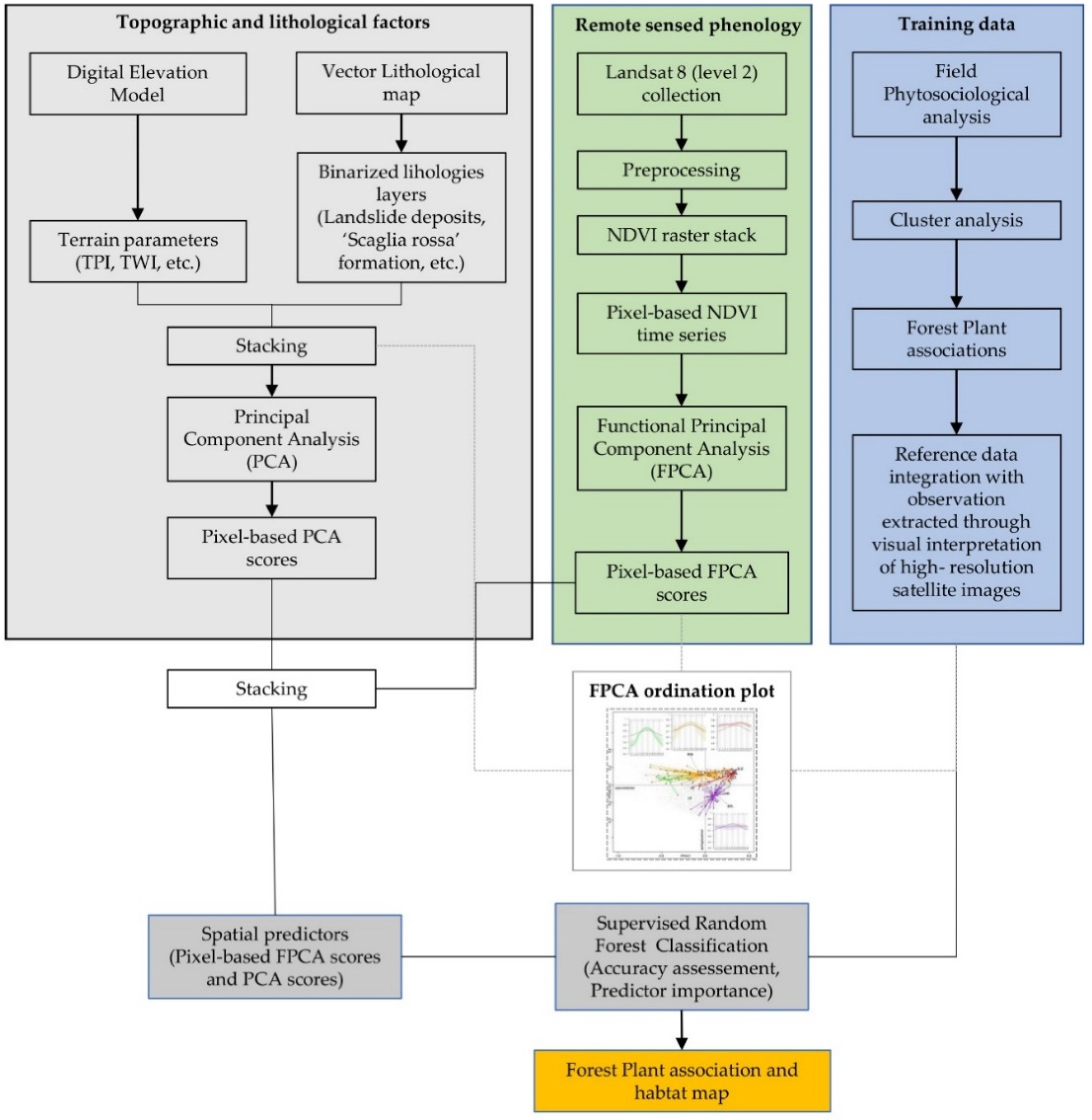
2. Materials and Methods
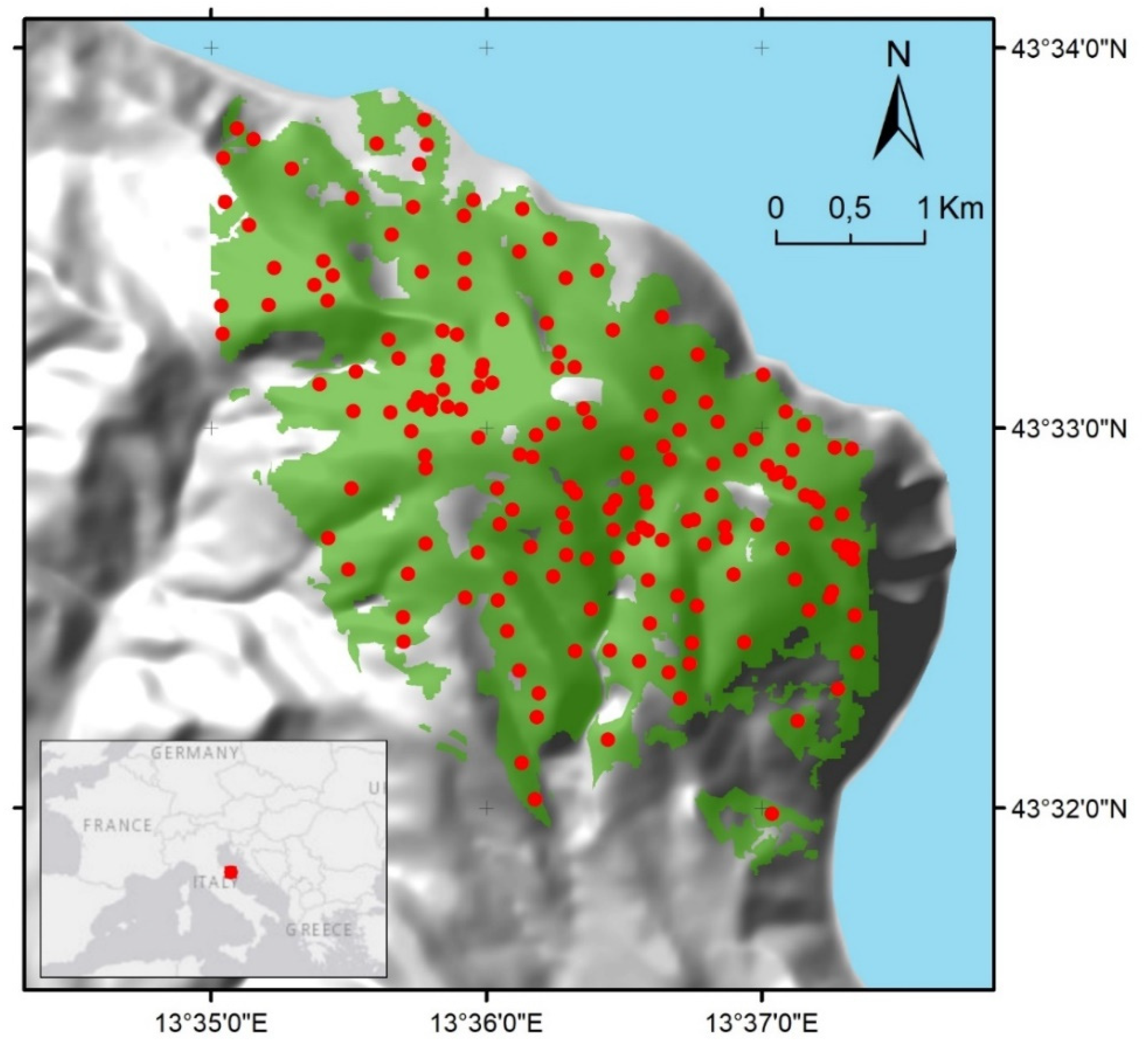
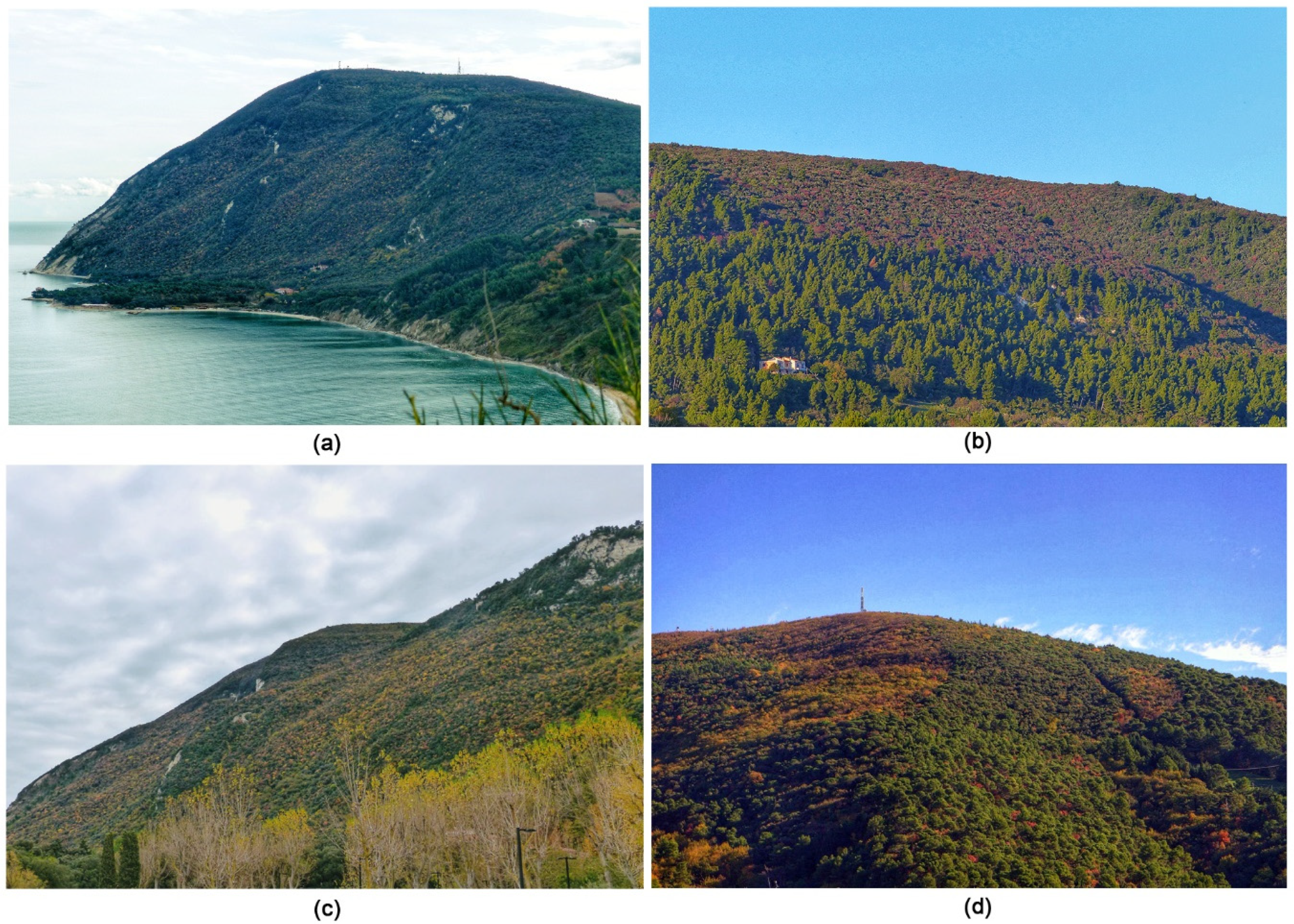
2.1. Study Site
2.2. Data Collection
2.2.1. Remote-Sensed NDVI Times Series
2.2.2. Functional Principal Component Analysis of NDVI Time Series
2.2.3. Topographic and Lithological Factors
2.2.4. Forest Plant Associations and Reference Data Collection
2.2.5. Relationships between NDVI Seasonality, Topography, and Forest Plant Associations
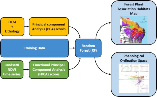
2.3. Supervised Mapping of the Forest Plant Associations
3. Results
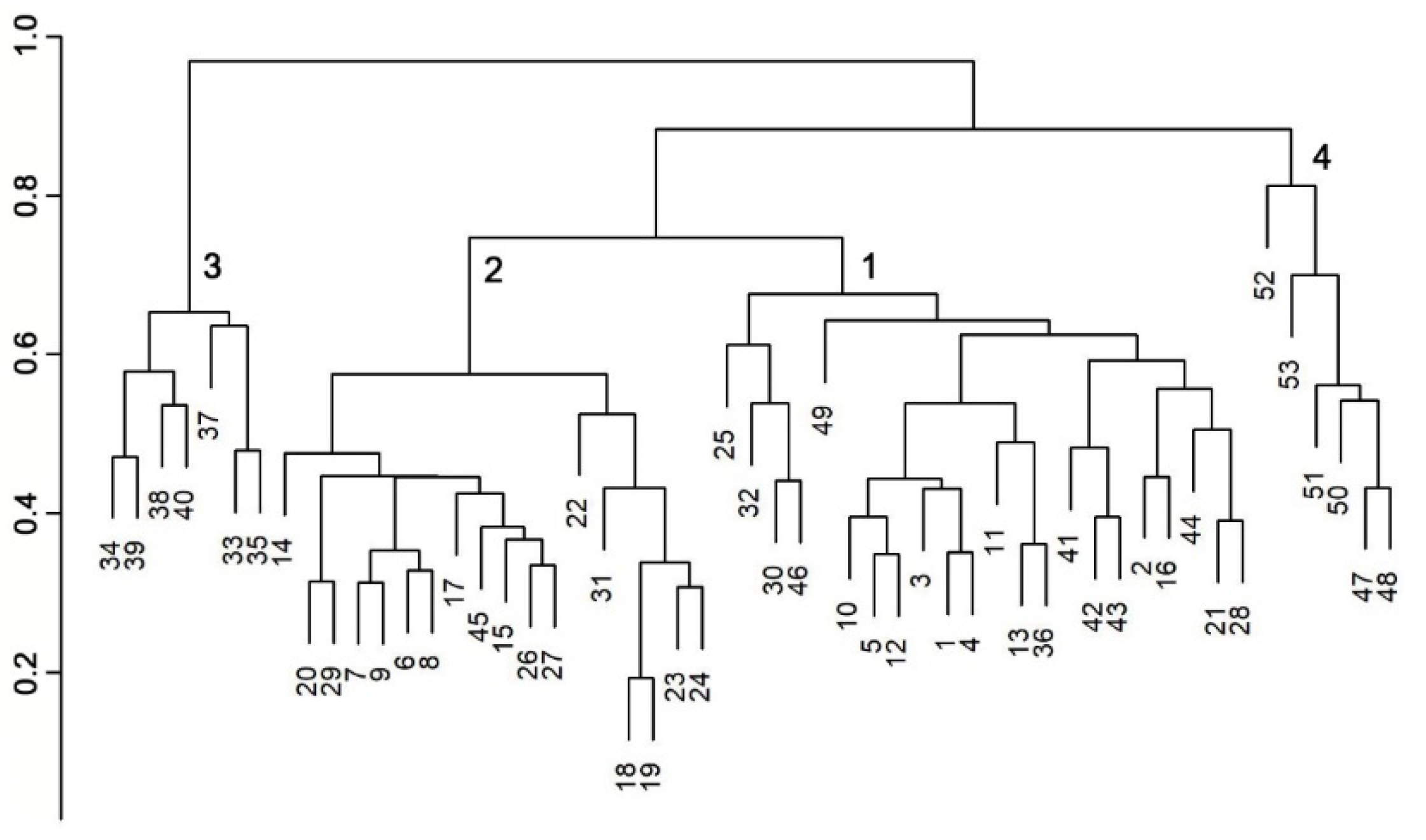
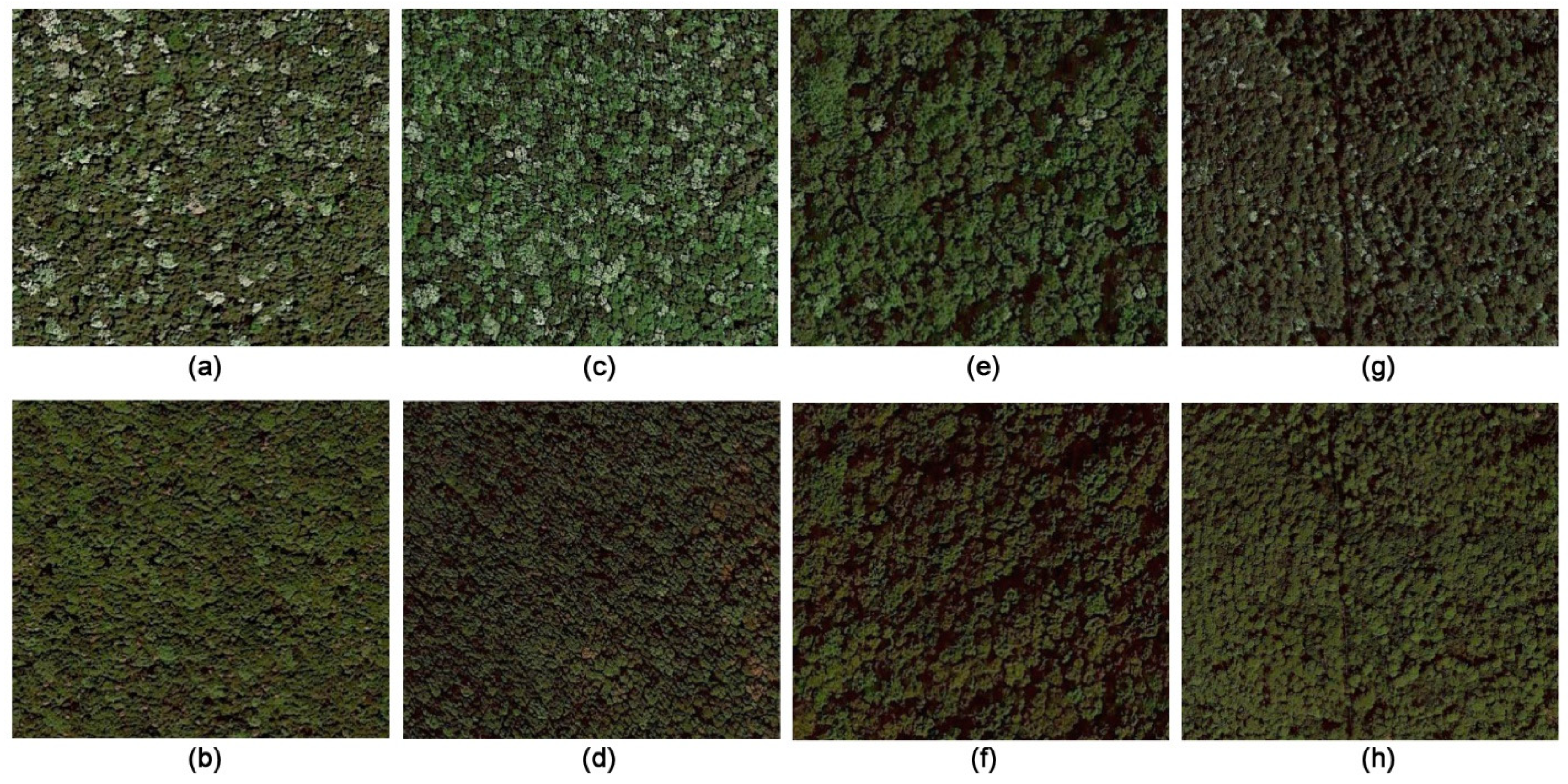
3.1. Forest Vegetation Field Survey and Plant Associations
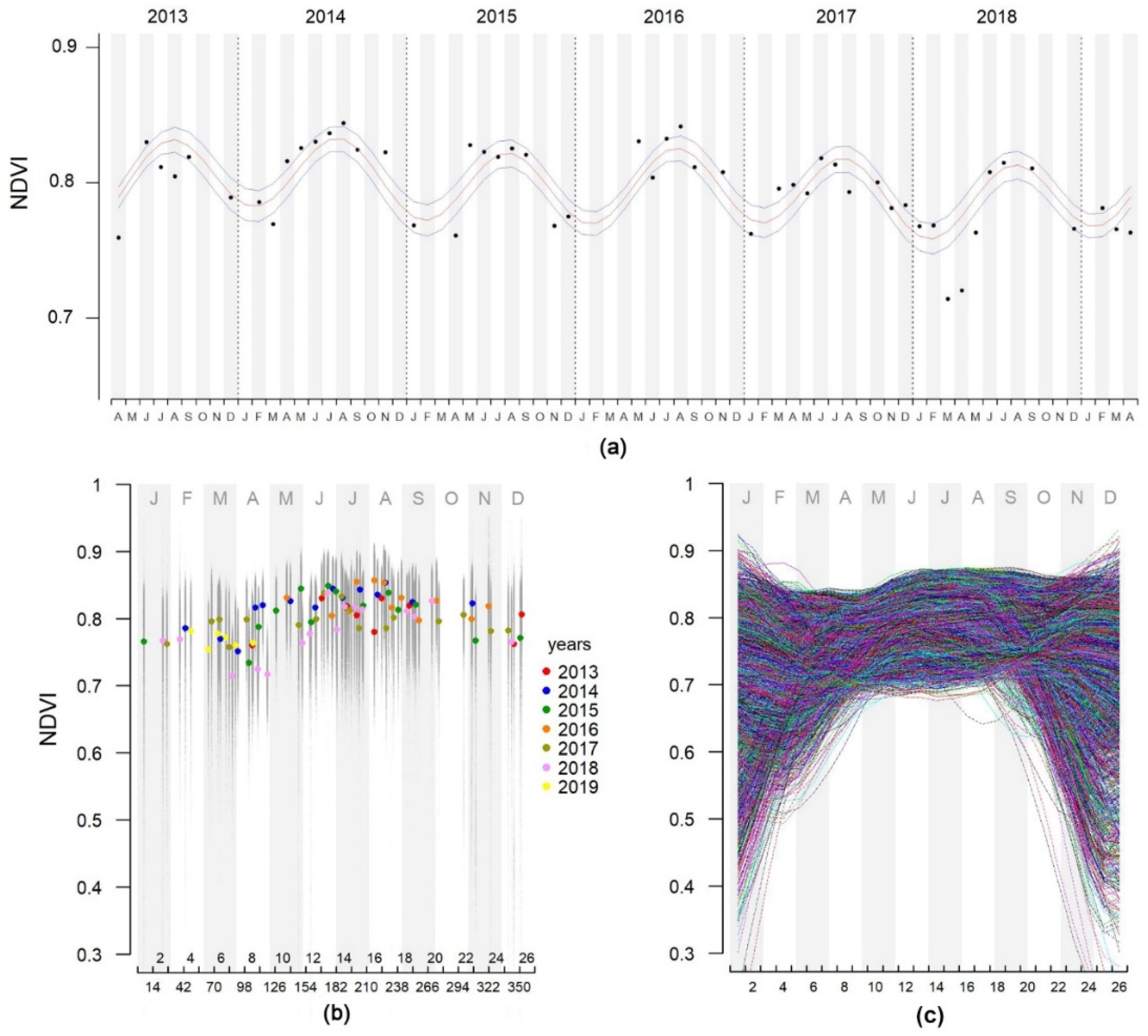
3.2. Main Seasonal NDVI Variation of the Forests
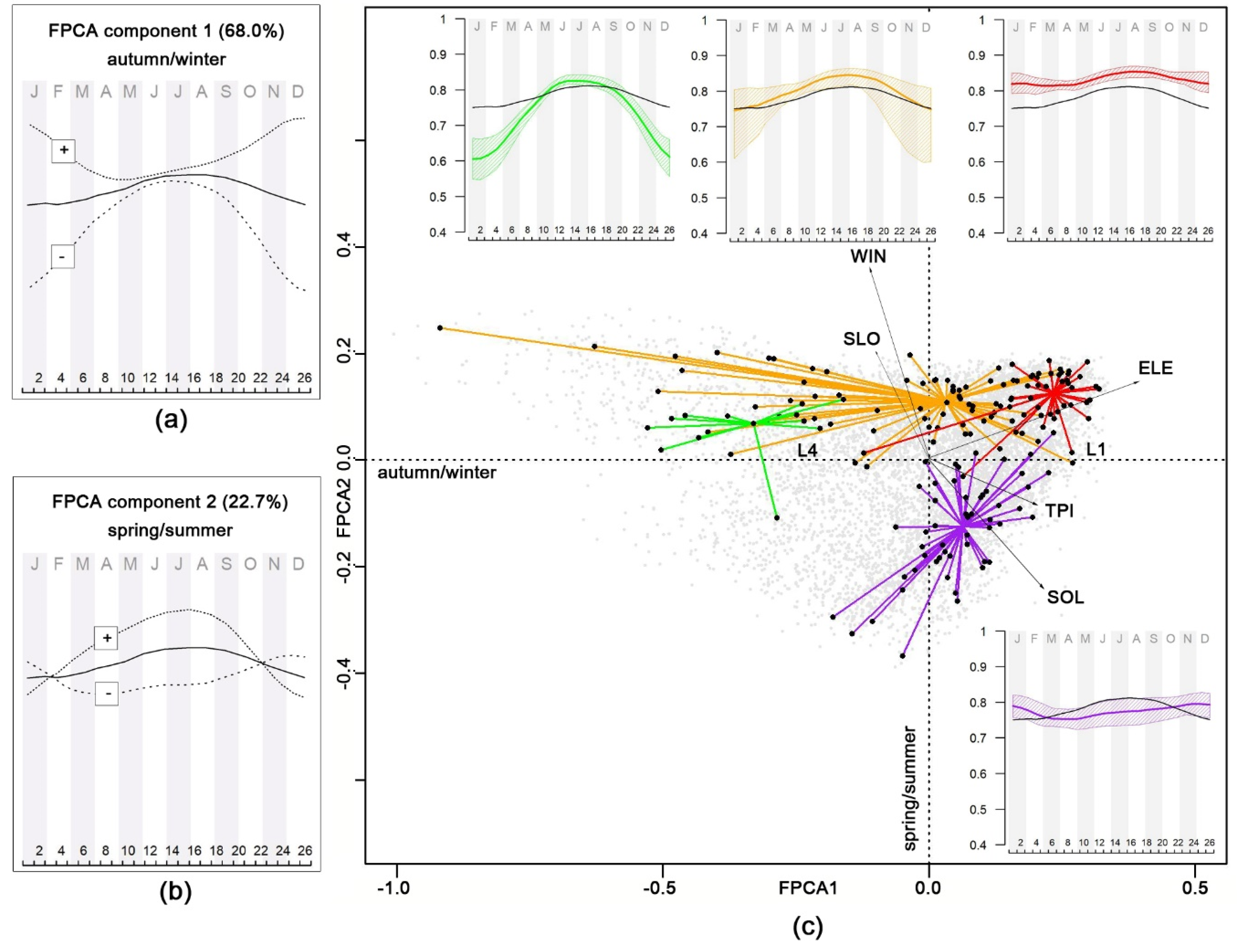
Relationships between NDVI Seasonality, Topography, and Forest Plant Associations
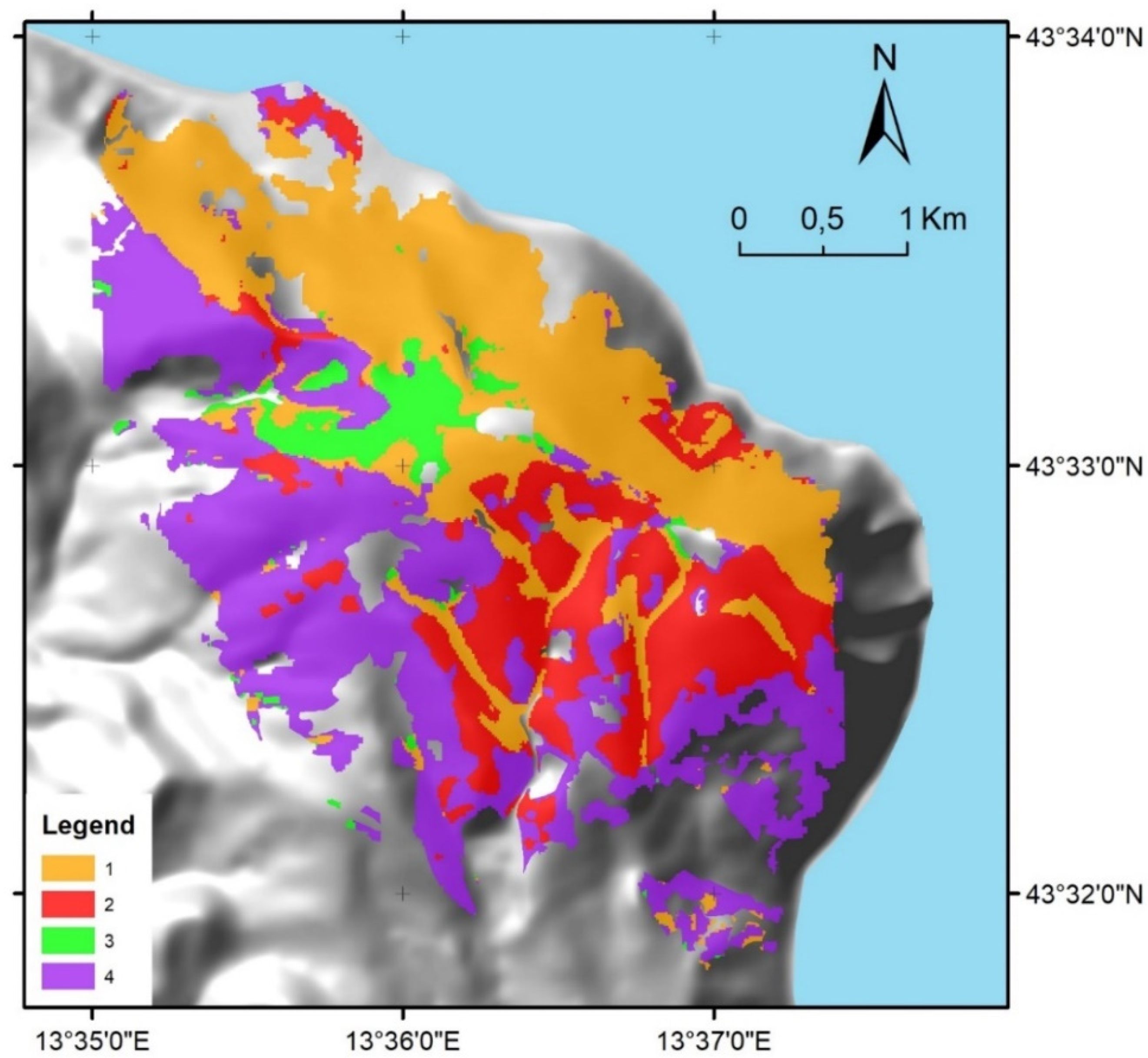
3.3. Phenology and Topography-Based Plant Association Map
4. Discussion
4.1. Mapping Performance and Methodological Considerations
4.2. Some Considerations of the Limits of This Study and Future Works
5. Conclusions
Author Contributions
Funding
Conflicts of Interest
Appendix A

| Plant Association | 3 | 1 | 2 | 4 |
|---|---|---|---|---|
| Number of plots (pixels) | 7 | 22 | 18 | 6 |
| Mean Richness (±SD) of groups | 27.7 | 16 | 13.6 | 15.1 |
| (±4.9) | (±3.2) | (±2.5) | (±4.4) | |
| Primula vulgaris | 43 | |||
| Stachys officinalis | 57 | |||
| Campanula trachelium | 29 | |||
| Solidago virgaurea | 29 | |||
| Brachypodium sylvaticum | 71 | |||
| Buglossoides purpurocaerulea | 71 | |||
| Euonymus europaeus | 29 | 17 | ||
| Cornus mas | 29 | |||
| Sanicula europaea | 29 | |||
| Epipactis helleborine | 43 | 9 | 11 | |
| Hepatica nobilis | 57 | 9 | ||
| Cornus sanguinea | 71 | 9 | ||
| Crataegus monogyna | 71 | 9 | 33 | |
| Viola reichenbachiana | 71 | 5 | ||
| Melittis melissophyllum | 86 | 14 | ||
| Viola alba ssp. dehnhardtii | 100 | 32 | 6 | |
| Lonicera etrusca | 100 | 5 | 6 | 17 |
| Carex halleriana | 100 | 5 | 6 | 50 |
| Daphne laureola | 100 | 45 | 17 | 33 |
| Acer obtusatum | 100 | 59 | 6 | 33 |
| Quercus virgiliana | 100 | 50 | 44 | 100 |
| Ostrya carpinifolia | 100 | 100 | 17 | |
| Cyclamen repandum | 29 | 50 | ||
| Ilex aquifolium | 36 | 17 | ||
| Mercurialis perennis | 32 | |||
| Quercus ilex | 100 | 100 | 100 | 100 |
| Phillyrea media | 9 | 44 | ||
| Osyris alba | 14 | 61 | 17 | |
| Pistacia lentiscus | 50 | 17 | ||
| Arbutus unedo | 50 | 100 | 50 | |
| Pinus pinea | 5 | 67 | ||
| Pinus halepensis | 5 | 11 | 100 | |
| Cyclamen hederifolium | 43 | 45 | 22 | |
| Ruscus hypoglossum | 14 | 50 | 6 | |
| Sorbus domestica | 43 | 14 | 17 | |
| Sorbus torminalis | 14 | 27 | 6 | |
| Cephalanthera longifolia | 29 | 5 | 11 | |
| Juniperus oxycedrus | 39 | 33 | ||
| Hedera helix | 100 | 86 | 44 | 33 |
| Viburnum tinus | 29 | 95 | 100 | 100 |
| Smilax aspera | 86 | 100 | 100 | 67 |
| Rubia peregrina | 100 | 77 | 72 | 83 |
| Ruscus aculeatus | 86 | 100 | 100 | 50 |
| Fraxinus ornus | 100 | 100 | 100 | 100 |
| Asparagus acutifolius | 100 | 77 | 100 | 83 |
| Coronilla emerus ssp. emeroides | 86 | 50 | 83 | 17 |
| Rosa sempervirens | 57 | 36 | 50 | 50 |
| Laurus nobilis | 14 | 36 | 6 | 17 |
| Brachypodium rupestre | 57 | 5 | 67 | |
| Rubus ulmifolius | 57 | 9 | 67 | |
| Prunus avium | 29 | 17 |
| Acquisition Date | DoY | Week | Be-Week | Month | Year |
|---|---|---|---|---|---|
| 06/01/2015 | 6 | 1 | 1 | 1 | 2015 |
| 23/01/2018 | 23 | 4 | 2 | 1 | 2018 |
| 27/01/2017 | 27 | 4 | 2 | 1 | 2017 |
| 08/02/2018 | 39 | 6 | 3 | 2 | 2018 |
| 13/02/2014 | 44 | 7 | 4 | 2 | 2014 |
| 18/02/2019 | 49 | 7 | 4 | 2 | 2019 |
| 06/03/2019 | 65 | 10 | 5 | 3 | 2019 |
| 09/03/2017 | 68 | 10 | 5 | 3 | 2017 |
| 15/03/2019 | 74 | 11 | 6 | 3 | 2019 |
| 16/03/2017 | 75 | 11 | 6 | 3 | 2017 |
| 17/03/2014 | 76 | 11 | 6 | 3 | 2014 |
| 22/03/2019 | 81 | 12 | 6 | 3 | 2019 |
| 25/03/2017 | 84 | 12 | 6 | 3 | 2017 |
| 28/03/2018 | 87 | 13 | 7 | 3 | 2018 |
| 31/03/2019 | 90 | 13 | 7 | 3 | 2019 |
| 02/04/2014 | 92 | 14 | 7 | 4 | 2014 |
| 10/04/2017 | 100 | 15 | 8 | 4 | 2017 |
| 12/04/2015 | 102 | 15 | 8 | 4 | 2015 |
| 15/04/2013 | 105 | 15 | 8 | 4 | 2013 |
| 16/04/2019 | 106 | 16 | 8 | 4 | 2019 |
| 18/04/2014 | 108 | 16 | 8 | 4 | 2014 |
| 20/04/2018 | 110 | 16 | 8 | 4 | 2018 |
| 21/04/2015 | 111 | 16 | 8 | 4 | 2015 |
| 25/04/2014 | 115 | 17 | 9 | 4 | 2014 |
| 29/04/2018 | 119 | 17 | 9 | 4 | 2018 |
| 07/05/2015 | 127 | 19 | 10 | 5 | 2015 |
| 16/05/2016 | 137 | 20 | 10 | 5 | 2016 |
| 20/05/2014 | 140 | 20 | 10 | 5 | 2014 |
| 28/05/2017 | 148 | 22 | 11 | 5 | 2017 |
| 30/05/2015 | 150 | 22 | 11 | 5 | 2015 |
| 31/05/2018 | 151 | 22 | 11 | 5 | 2018 |
| 07/06/2018 | 158 | 23 | 12 | 6 | 2018 |
| 08/06/2015 | 159 | 23 | 12 | 6 | 2015 |
| 12/06/2014 | 163 | 24 | 12 | 6 | 2014 |
| 13/06/2017 | 164 | 24 | 12 | 6 | 2017 |
| 18/06/2013 | 169 | 25 | 13 | 6 | 2013 |
| 20/06/2017 | 171 | 25 | 13 | 6 | 2017 |
| 23/06/2018 | 174 | 25 | 13 | 6 | 2018 |
| 24/06/2015 | 175 | 25 | 13 | 6 | 2015 |
| 26/06/2016 | 178 | 26 | 13 | 6 | 2016 |
| 28/06/2014 | 179 | 26 | 13 | 6 | 2014 |
| 01/07/2015 | 182 | 26 | 13 | 7 | 2015 |
| 02/07/2018 | 183 | 27 | 14 | 7 | 2018 |
| 06/07/2017 | 187 | 27 | 14 | 7 | 2017 |
| 07/07/2014 | 188 | 27 | 14 | 7 | 2014 |
| 09/07/2018 | 190 | 28 | 14 | 7 | 2018 |
| 10/07/2015 | 191 | 28 | 14 | 7 | 2015 |
| 11/07/2013 | 192 | 28 | 14 | 7 | 2013 |
| 12/07/2016 | 194 | 28 | 14 | 7 | 2016 |
| 15/07/2017 | 196 | 28 | 14 | 7 | 2017 |
| 18/07/2018 | 199 | 29 | 15 | 7 | 2018 |
| 20/07/2013 | 201 | 29 | 15 | 7 | 2013 |
| 19/07/2016 | 201 | 29 | 15 | 7 | 2016 |
| 22/07/2017 | 203 | 29 | 15 | 7 | 2017 |
| 23/07/2014 | 204 | 30 | 15 | 7 | 2014 |
| 25/07/2018 | 206 | 30 | 15 | 7 | 2018 |
| 26/07/2015 | 207 | 30 | 15 | 7 | 2015 |
| 05/08/2013 | 217 | 31 | 16 | 8 | 2013 |
| 04/08/2016 | 217 | 31 | 16 | 8 | 2016 |
| 08/08/2014 | 220 | 32 | 16 | 8 | 2014 |
| 12/08/2013 | 224 | 32 | 16 | 8 | 2013 |
| 13/08/2016 | 226 | 33 | 17 | 8 | 2016 |
| 15/08/2014 | 227 | 33 | 17 | 8 | 2014 |
| 16/08/2017 | 228 | 33 | 17 | 8 | 2017 |
| 18/08/2015 | 230 | 33 | 17 | 8 | 2015 |
| 20/08/2016 | 233 | 34 | 17 | 8 | 2016 |
| 23/08/2017 | 235 | 34 | 17 | 8 | 2017 |
| 27/08/2015 | 239 | 35 | 18 | 8 | 2015 |
| 29/08/2016 | 242 | 35 | 18 | 8 | 2016 |
| 04/09/2018 | 247 | 36 | 18 | 9 | 2018 |
| 06/09/2013 | 249 | 36 | 18 | 9 | 2013 |
| 09/09/2014 | 252 | 36 | 18 | 9 | 2014 |
| 11/09/2018 | 254 | 37 | 19 | 9 | 2018 |
| 12/09/2015 | 255 | 37 | 19 | 9 | 2015 |
| 14/09/2016 | 258 | 37 | 19 | 9 | 2016 |
| 27/09/2018 | 270 | 39 | 20 | 9 | 2018 |
| 30/09/2016 | 274 | 40 | 20 | 9 | 2016 |
| 03/10/2017 | 276 | 40 | 20 | 10 | 2017 |
| 26/10/2017 | 299 | 43 | 22 | 10 | 2017 |
| 01/11/2016 | 306 | 44 | 22 | 11 | 2016 |
| 03/11/2014 | 307 | 44 | 22 | 11 | 2014 |
| 06/11/2015 | 310 | 45 | 23 | 11 | 2015 |
| 17/11/2016 | 322 | 46 | 23 | 11 | 2016 |
| 20/11/2017 | 324 | 47 | 24 | 11 | 2017 |
| 06/12/2017 | 340 | 49 | 25 | 12 | 2017 |
| 09/12/2018 | 343 | 49 | 25 | 12 | 2018 |
| 11/12/2013 | 345 | 50 | 25 | 12 | 2013 |
| 17/12/2015 | 351 | 51 | 26 | 12 | 2015 |
| 18/12/2013 | 352 | 51 | 26 | 12 | 2013 |


References
- CEC Council Directive 92/43/EEC of 21 May 1992 on the conservation of natural habitats and of wild fauna and flora. Off. J. Eur. Union 1992, 206, 7–50.
- Evans, D. The habitats of the European Union Habitats Directive. Biol. Environ. Proc. R. Irish Acad. 2006, 106, 167–173. [Google Scholar] [CrossRef] [Green Version]
- Rodwell, J.S.; Evans, D.; Schaminée, J.H.J. Phytosociological relationships in European Union policy-related habitat classifications. Rend. Lincei 2018, 29, 237–249. [Google Scholar] [CrossRef]
- Biondi, E. Phytosociology today: Methodological and conceptual evolution. Plant Biosyst. 2011, 145, 19–29. [Google Scholar] [CrossRef]
- Biondi, E.; Burrascano, S.; Casavecchia, S.; Copiz, R.; Del Vico, E.; Galdenzi, D.; Gigante, D.; Lasen, C.; Spampinato, G.; Venanzoni, R.; et al. Diagnosis and syntaxonomic interpretation of Annex I Habitats (Dir. 92/43/EEC) in Italy at the alliance level. Plant Sociol. 2012, 49, 5–37. [Google Scholar]
- Gigante, D.; Attorre, F.; Venanzoni, R.; Acosta, A.T.R.; Agrillo, E.; Aleffi, M.; Alessi, N.; Allegrezza, M.; Angelini, P.; Angiolini, C.; et al. A methodological protocol for Annex I Habitats monitoring: The contribution of vegetation science. Plant Sociol. 2016, 53, 77–87. [Google Scholar]
- Frontoni, E.; Mancini, A.; Zingaretti, P.; Malinverni, E.; Pesaresi, S.; Biondi, E.; Pandolfi, M.; Marseglia, M.; Sturari, M.; Zabaglia, C. SIT-REM: An Interoperable and Interactive Web Geographic Information System for Fauna, Flora and Plant Landscape Data Management. ISPRS Int. J. Geo-Inf. 2014, 3, 853–867. [Google Scholar] [CrossRef] [Green Version]
- Viciani, D.; Dell’Olmo, L.; Ferretti, G.; Lazzaro, L.; Lastrucci, L.; Foggi, B. Detailed Natura 2000 and CORINE Biotopes habitat maps of the island of Elba (Tuscan Archipelago, Italy). J. Maps 2016, 12, 492–502. [Google Scholar] [CrossRef]
- Ichter, J.; Savio, L.; Evans, D.; Poncet, L. State-of-the-art of vegetation mapping in Europe: Results of a European survey and contribution to the French program CarHAB. Doc. Phytosociol. Série 3 2017, 6, 335–352. [Google Scholar]
- Ichter, J.; Evans, D.; Richard, D. Terrestrial Habitat Mapping in Europe: An Overview; Poncet, L., Spyropoulou, R., Martins, I.P., Eds.; MNHN-EEA: Luxembourg, 2014; Volume 1, pp. 7–154. ISBN 978-92-9213-420-4. [Google Scholar]
- Vanden Borre, J.; Paelinckx, D.; Mücher, C.A.; Kooistra, L.; Haest, B.; De Blust, G.; Schmidt, A.M. Integrating remote sensing in Natura 2000 habitat monitoring: Prospects on the way forward. J. Nat. Conserv. 2011, 19, 116–125. [Google Scholar] [CrossRef]
- Corbane, C.; Lang, S.; Pipkins, K.; Alleaume, S.; Deshayes, M.; García Millán, V.E.; Strasser, T.; Vanden Borre, J.; Toon, S.; Michael, F. Remote sensing for mapping natural habitats and their conservation status—New opportunities and challenges. Int. J. Appl. Earth Obs. Geoinf. 2015, 37, 7–16. [Google Scholar] [CrossRef]
- Zlinszky, A.; Deák, B.; Kania, A.; Schroiff, A.; Pfeifer, N. Mapping natura 2000 habitat conservation status in a pannonic salt steppe with airborne laser scanning. Remote Sens. 2015, 7, 2991–3019. [Google Scholar] [CrossRef] [Green Version]
- Rouse, J.W., Jr.; Haas, R.H.; Schell, J.A.; Deering, D.W. Monitoring Vegetation Systems in the Great Plains with ERTS; NASA. Goddard Space Flight Center 3d ERTS-1 Symp.; SEE 19740022592, Sect. A; NASA: Washington, DC, USA, 1974; Volume 1, pp. 309–317. [Google Scholar]
- White, M.A.; Hoffman, F.; Hargrove, W.W.; Nemani, R.R. A global framework for monitoring phenological responses to climate change. Geophys. Res. Lett. 2005, 32, L04705. [Google Scholar] [CrossRef] [Green Version]
- Feret, J.B.; Corbane, C.; Alleaume, S. Detecting the Phenology and Discriminating Mediterranean Natural Habitats with Multispectral Sensors-An Analysis Based on Multiseasonal Field Spectra. IEEE J. Sel. Top. Appl. Earth Obs. Remote Sens. 2015, 8, 2294–2305. [Google Scholar] [CrossRef]
- Grignetti, A.; Salvatori, R.; Casacchia, R.; Manes, F. Mediterranean vegetation analysis by multi-temporal satellite sensor data. Int. J. Remote Sens. 1997, 18, 1307–1318. [Google Scholar] [CrossRef]
- Alcaraz-Segura, D.; Cabello, J.; Paruelo, J. Baseline characterization of major Iberian vegetation types based on the NDVI dynamics. Plant Ecol. 2009, 202, 13–29. [Google Scholar] [CrossRef]
- Marzialetti, F.; Giulio, S.; Malavasi, M.; Sperandii, M.G.; Acosta, A.T.R.; Carranza, M.L. Capturing Coastal Dune Natural Vegetation Types Using a Phenology-Based Mapping Approach: The Potential of Sentinel-2. Remote Sens. 2019, 11, 1506. [Google Scholar] [CrossRef] [Green Version]
- Rapinel, S.; Mony, C.; Lecoq, L.; Clément, B.; Thomas, A.; Hubert-Moy, L. Evaluation of Sentinel-2 time-series for mapping floodplain grassland plant communities. Remote Sens. Environ. 2019, 223, 115–129. [Google Scholar] [CrossRef]
- Rivas-Martínez, S.; Sáenz, S.R.; Penas, A. Worldwide bioclimatic classification system. Glob. Geobot. 2011, 1, 1–634. [Google Scholar]
- Pesaresi, S.; Biondi, E.; Casavecchia, S. Bioclimates of Italy. J. Maps 2017, 13, 955–960. [Google Scholar] [CrossRef]
- Biondi, E. L’ostrya carpinifolia scop. sul litorale delle Marche (Italia centrale). Stud. Geobot. 1982, 2, 141–147. [Google Scholar]
- Biondi, E. La Vegetazione del Monte Conero (Con Carta della Vegetazione alla Scala 1:10000); Biondi, E., Ed.; Tecnostampa: Ostra Vetere, Italy, 1986. [Google Scholar]
- Biondi, E.; Gubellini, L.; Pinzi, M.; Casavecchia, S. The vascular flora of Conero Regional Nature Park (Marche, Central Italy). Flora Mediterr. 2012, 22, 67–167. [Google Scholar] [CrossRef]
- Baiocco, M.; Casavecchia, S.; Biondi, E.; Pietracapina, A. Indagini Geobotaniche per il recupero del Rimboschimento del Monte Conero (Italia Centrale). Doc. Phytosociol. NS 1996, XVI, 389–392. [Google Scholar]
- Angelini, P.; Casella, L.; Grignetti, A.; Genovesi, P. Manuali per il Monitoraggio di Specie e Habitat di Interesse Comunitario (Direttiva 92/43/CEE) in Italia: Habitat; Serie Manuali e linee guida, 142/2016; ISPRA: Rome, Italy, 2016; pp. 1–280. ISBN 978-88-448-0789-4. [Google Scholar]
- O’Neill, R.V.; Hunsaker, C.T.; Timmins, S.P.; Jackson, B.L.; Jones, K.B.; Riitters, K.H.; Wickham, J.D. Scale problems in reporting landscape pattern at the regional scale. Landsc. Ecol. 1996, 11, 169–180. [Google Scholar] [CrossRef]
- Soenen, S.A.; Peddle, D.R.; Coburn, C.A. SCS + C: A modified Sun-canopy-sensor topographic correction in forested terrain. IEEE Trans. Geosci. Remote Sens. 2005, 43, 2148–2159. [Google Scholar] [CrossRef]
- Leutner, B.; Horning, N.; Schwalb-Willmann, J. RStoolbox: Tools for Remote Sensing Data Analysis. R Package Version 0.2.3. Available online: https://cran.r-project.org/package=RStoolbox (accessed on 1 April 2020).
- Hyndman, R.; Athanasopoulos, G.; Bergmeir, C.; Caceres, G.; Chhay, L.; O’Hara-Wild, M.; Petropoulos, F.; Razbash, S.; Wang, E.; Yasmeen, F. forecast: Forecasting Functions for Time Series and Linear Models. R Package Version 8.6. Available online: https://cran.r-project.org/package=forecast (accessed on 1 April 2020).
- Hyndman, R.J.; Khandakar, Y. Automatic Time Series Forecasting: The forecast Package for R. J. Stat. Softw. 2008, 27, 1–22. [Google Scholar] [CrossRef] [Green Version]
- Ramsay, J.O.; Silverman, B.W. Functional Data Analysis; Ramsay, R., Silverman, B., Eds.; Springer: New York, NY, USA, 2005; ISBN 978-0-387-40080-8. [Google Scholar]
- Hurley, M.A.; Hebblewhite, M.; Gaillard, J.; Dray, S.; Taylor, K.A.; Smith, W.K.; Zager, P.; Bonenfant, C. Functional analysis of normalized difference vegetation index curves reveals overwinter mule deer survival is driven by both spring and autumn phenology. Philos. Trans. R. Soc. Lond. B. Biol. Sci. 2014, 369, 20130196. [Google Scholar] [CrossRef] [Green Version]
- Wang, J.-L.; Chiou, J.-M.; Müller, H.-G. Functional Data Analysis. Annu. Rev. Stat. Appl. 2016, 3, 257–295. [Google Scholar] [CrossRef] [Green Version]
- Yao, F.; Müller, H.G.; Wang, J.L. Functional data analysis for sparse longitudinal data. J. Am. Stat. Assoc. 2005, 100, 577–590. [Google Scholar] [CrossRef]
- Dai, X.; Hadjipantelis, P.Z.; Han, K.; Ji, H. fdapace: Functional Data Analysis and Empirical Dynamics. R Package Version 0.4.0. Available online: https://cran.r-project.org/package=fdapace (accessed on 1 April 2020).
- Tardella, F.M.; Postiglione, N.; Vitanzi, A.; Catorci, A. The effects of environmental features and overstory composition on the understory species assemblage in sub-mediterranean coppiced woods: Implications for a sustainable forest management. Polish J. Ecol. 2017, 65, 167–182. [Google Scholar] [CrossRef]
- Dubeau, P.; King, D.J.; Unbushe, D.G.; Rebelo, L.M. Mapping the Dabus Wetlands, Ethiopia, using random forest classification of Landsat, PALSAR and topographic data. Remote Sens. 2017, 9, 1056. [Google Scholar] [CrossRef] [Green Version]
- Marcinkowska-Ochtyra, A.; Gryguc, K.; Ochtyra, A.; Kopeć, D.; Jarocińska, A.; Sławik, Ł. Multitemporal Hyperspectral Data Fusion with Topographic Indices—Improving Classification of Natura 2000 Grassland Habitats. Remote Sens. 2019, 11, 2264. [Google Scholar] [CrossRef] [Green Version]
- Conrad, O.; Bechtel, B.; Bock, M.; Dietrich, H.; Fischer, E.; Gerlitz, L.; Wehberg, J.; Wichmann, V.; Böhner, J. System for Automated Geoscientific Analyses (SAGA) v. 2.1.4. Geosci. Model Dev. 2015, 8, 1991–2007. [Google Scholar] [CrossRef] [Green Version]
- Böhner, J.; Antonić, O. Land-Surface Parameters Specific to Topo-Climatology. In Developments in Soil Science; Chapter 8; Hengl, T., Reuter, H.I., Eds.; Elsevier: Amsterdam, The Netherlands, 2009; pp. 195–226. [Google Scholar]
- Marche, R. La Carta Geologica della Regione Marche in Scala 1:10.000. Available online: http://www.regione.marche.it/Regione-Utile/Paesaggio-Territorio-Urbanistica/Cartografia/Repertorio/Cartageologicaregionale10000 (accessed on 1 April 2020).
- Guisan, A.; Weiss, S.B.; Weiss, A.D. GLM versus CCA spatial modeling of plant species distribution. Plant Ecol. 1999, 143, 107–122. [Google Scholar] [CrossRef]
- Dengler, J. Phytosociology. In International Encyclopedia of Geography: People, the Earth, Environment and Technology; Richardson, D., Castree, N., Goodchild, M.F., Kobayashi, A., Liu, W., Marston, R.A., Eds.; John Wiley & Sons, Ltd: Oxford, UK, 2017; pp. 1–6. ISBN 9781118786352. [Google Scholar]
- Braun-Blanquet, J.; Conard, H.S.; Fuller, G.D. Plant Sociology; The Study of Plant Communities, 1st ed.; Conard, H.S., Fuller, G.D., Eds.; McGraw-Hill Inc.: New York, NY, USA, 1932. [Google Scholar]
- Biondi, E.; Casavecchia, S.; Pesaresi, S. Phytosociological synrelevés and plant landscape mapping: From theory to practice. Plant Biosyst. 2011, 145, 261–273. [Google Scholar] [CrossRef]
- De Cáceres, M.; Legendre, P. Associations between species and groups of sites: Indices and statistical inference. Ecology 2009, 90, 3566–3574. [Google Scholar] [CrossRef]
- Oksanen, J.; Blanchet, F.G.; Friendly, M.; Kindt, R.; Legendre, P.; McGlinn, D.; Minchin, P.R.; O’Hara, R.B.; Simpson, G.L.; Solymos, P.; et al. Vegan: Community Ecology Package. R Package Version 2.5-3. Available online: https://cran.r-project.org/package=vegan (accessed on 1 April 2020).
- Breiman, L. Random Forests. Mach. Learn. 2001, 45, 5–32. [Google Scholar] [CrossRef] [Green Version]
- Belgiu, M.; Drăguţ, L. Random forest in remote sensing: A review of applications and future directions. ISPRS J. Photogramm. Remote Sens. 2016, 114, 24–31. [Google Scholar] [CrossRef]
- Evans, J.S.; Cushman, S.A. Gradient modeling of conifer species using random forests. Landsc. Ecol. 2009, 24, 673–683. [Google Scholar] [CrossRef]
- Hijmans, R.J. Raster: Geographic Data Analysis and Modeling. R Package Version 2.8-4. Available online: https://cran.r-project.org/package=raster (accessed on 1 April 2020).
- Kuhn, M. Building Predictive Models in R Using the caret Package. J. Stat. Softw. 2008, 28, 1–26. [Google Scholar] [CrossRef] [Green Version]
- Zhu, X.; Liu, D. Accurate mapping of forest types using dense seasonal landsat time-series. ISPRS J. Photogramm. Remote Sens. 2014, 96, 1–11. [Google Scholar] [CrossRef]
- Zlinszky, A.; Heilmeier, H.; Balzter, H.; Czúcz, B.; Pfeifer, N. Remote sensing and GIS for habitat quality monitoring: New approaches and future research. Remote Sens. 2015, 7, 7987–7994. [Google Scholar] [CrossRef] [Green Version]
- Bajocco, S.; Ferrara, C.; Alivernini, A.; Bascietto, M.; Ricotta, C. Remotely-sensed phenology of Italian forests: Going beyond the species. Int. J. Appl. Earth Obs. Geoinf. 2019, 74, 314–321. [Google Scholar] [CrossRef]
- Bajocco, S.; Dragoz, E.; Gitas, I.; Smiraglia, D.; Salvati, L.; Ricotta, C. Mapping Forest Fuels through Vegetation Phenology: The Role of Coarse-Resolution Satellite Time-Series. PLoS ONE 2015, 10, e0119811. [Google Scholar] [CrossRef] [Green Version]
- De Cáceres, M.; Chytrý, M.; Agrillo, E.; Attorre, F.; Botta-Dukát, Z.; Capelo, J.; Czúcz, B.; Dengler, J.; Ewald, J.; Faber-Langendoen, D.; et al. A comparative framework for broad-scale plot-based vegetation classification. Appl. Veg. Sci. 2015, 18, 543–560. [Google Scholar] [CrossRef] [Green Version]
- Riaño, D.; Chuvieco, E.; Salas, J.; Aguado, I. Assessment of different topographic corrections in landsat-TM data for mapping vegetation types (2003). IEEE Trans. Geosci. Remote Sens. 2003, 41, 1056–1061. [Google Scholar] [CrossRef] [Green Version]
- Duckworth, J.C.; Kent, M.; Ramsay, P.M. Plant functional types: An alternative to taxonomic plant community description in biogeography? Prog. Phys. Geogr. Earth Environ. 2000, 24, 515–542. [Google Scholar] [CrossRef]


| Acronym | Description |
|---|---|
| ELEV | Altitude (m a.s.l) |
| SLO | Slope of the terrain (°) |
| SOL | Potential Incoming Solar Radiation. It characterizes the insolation intensity variation of the study area determined by the topography assuming uniform albedo and clear sky conditions. It was Calculated by the Module “Potential Incoming Solar Radiation” |
| WIN | Effect of the cold wind “Bora” that has a North-East direction, calculated by the Module “Wind Effect (Windward/Leeward Index)” |
| TWI | Topographic Wetness Index. It is a parameter describing the tendency of a cell to accumulate water and it is useful to characterize the wetness of the landscape. It was calculated by the module “SAGA Wetness Index” |
| TPI | Multi-Scale Topographic Position Index. Integrates in one single grid the Topographic Position Index (TPI) as proposed by Guisan et al. [44] calculated for different scales. It was calculated by the Module “Multi-Scale Topographic Position Index” |
| L | Lithologies (L1: “scaglia rossa” formation; L2: “scaglia variegata” formation; L3: “Maiolica” formation; L4: landslide deposit; L5: slope deposit) |
| Plant Associations | Training Data | ||
|---|---|---|---|
| Phytosociological Analysis | Visual Interpretation of Images | Total | |
| Cephalanthero longifoliae-Quercetum ilicis | 29 (22) | 43 | 72 |
| Cyclamino hederifolii-Quercetum ilicis | 18 (18) | 19 | 37 |
| Asparago acutifolii–Ostryetum carpinifoliae | 11 (7) | 2 | 13 |
| Pinus sp. plantation | 22 (6) | 31 | 53 |
| Training Data | ||||||
|---|---|---|---|---|---|---|
| Plant Association | 1 | 2 | 3 | 4 | User’s Accuracy (%) | |
| Prediction | 1 | 39.4 | 3.7 | 4.3 | 0.9 | 81.6 |
| 2 | 1.4 | 17.3 | 0.0 | 1.7 | 84.8 | |
| 3 | 0.1 | 0.0 | 3.1 | 0.0 | 96.8 | |
| 4 | 0.3 | 0.1 | 0.0 | 27.7 | 98.5 | |
| Producer’s accuracy (%) | 95.6 | 82.0 | 42.0 | 91.4 | ||
| Overall accuracy (%) | 87.5 | |||||
| Kappa statistic (%) | 0.81 | |||||
© 2020 by the authors. Licensee MDPI, Basel, Switzerland. This article is an open access article distributed under the terms and conditions of the Creative Commons Attribution (CC BY) license (http://creativecommons.org/licenses/by/4.0/).
Share and Cite
Pesaresi, S.; Mancini, A.; Quattrini, G.; Casavecchia, S. Mapping Mediterranean Forest Plant Associations and Habitats with Functional Principal Component Analysis Using Landsat 8 NDVI Time Series. Remote Sens. 2020, 12, 1132. https://0-doi-org.brum.beds.ac.uk/10.3390/rs12071132
Pesaresi S, Mancini A, Quattrini G, Casavecchia S. Mapping Mediterranean Forest Plant Associations and Habitats with Functional Principal Component Analysis Using Landsat 8 NDVI Time Series. Remote Sensing. 2020; 12(7):1132. https://0-doi-org.brum.beds.ac.uk/10.3390/rs12071132
Chicago/Turabian StylePesaresi, Simone, Adriano Mancini, Giacomo Quattrini, and Simona Casavecchia. 2020. "Mapping Mediterranean Forest Plant Associations and Habitats with Functional Principal Component Analysis Using Landsat 8 NDVI Time Series" Remote Sensing 12, no. 7: 1132. https://0-doi-org.brum.beds.ac.uk/10.3390/rs12071132