Spatially Variable Relationships between Karst Landscape Pattern and Vegetation Activities


1
Key Laboratory of Land Surface Pattern and Simulation, Institute of Geographic Sciences and Natural Resources Research, CAS, Beijing 100101, China
2
Academy of Plateau Science and Sustainability, Xining 810016, China
*
Author to whom correspondence should be addressed.
Remote Sens. 2020, 12(7), 1134; https://0-doi-org.brum.beds.ac.uk/10.3390/rs12071134
Submission received: 28 February 2020
/
Revised: 29 March 2020
/
Accepted: 1 April 2020
/
Published: 2 April 2020
(This article belongs to the Special Issue Ecosystem Services with Remote Sensing)
Abstract
:Based on the theories of structure–function correlation in Geography, and landscape pattern-ecological function correlation in Landscape Ecology, the correlation between land use fragmentation and vegetation activity was quantified. Effective mesh size (meff) was calculated to represent landscape fragmentation for land use, and the normalized difference vegetation index (NDVI) was used to reflect vegetation activity. The geographically weighted regression (GWR) model was applied to explore the spatial non-stationary relationship between meff and NDVI in a karst basin of the southwestern China, where environmental factors (i.e., climate, topography, and vegetation) are spatially heterogeneous. The spatial variation and scale dependence of landscape fragmentation and its relationship with vegetation activity, as well as the influence of lithology types and landforms relief, were considered. Firstly, the optimal ‘slide window’ size for landscape fragmentation was determined to be 500 m, and spatial pattern of meff displayed clear heterogeneity with a serious degree of fragmentation. Landscape fragmentation was more severe in carbonate areas than non-carbonate areas, reflecting the influence of landforms relief. More serious fragmentation in dolomite areas meant that the impact of human activities on the landscape morphological characteristics was much more significant than that in the limestone areas with steeper slope. Multi-scale analysis was used to verify a neighborhood size of 7 km for GWR in the study area. Negative effects on vegetation activity from landscape structural changes were more significant in limestone areas, which may be due to the more vulnerable ecosystems there. This research can provide scientific guidance for landscape management in karst regions as it considers the multi-scaled and spatially heterogeneous effects of lithology, geomorphology, and human factors on landscape structure and its correlation with vegetation activity.

1. Introduction
The structure–function correlation is a basic principle of geographic research [1,2], of which coupled studies on landscape patterns and ecological function in Landscape Ecology [3] are an important aspect. Most previous studies on the influence of land use on ecological function or vegetation activity have mainly focused on the type transformation and quality alteration [4,5,6]. For example, satellite-based vegetation indices and land use maps were applied to analyze the spatio-temporal difference in vegetation coverage among different land use types [7]. A field survey and model simulations were also combined to reveal the statistical relationships between land use and vegetation growth [8]. Furthermore, although landscape pattern indices have been widely applied to calculate land use structure [9], a quantitative investigation on the effects of land use changes on vegetation activity by embedding landscape indices has not attracted sufficient attention [10].
Many studies have pointed out that vegetation coverage, productivity and other indicators reflect the status of vegetation activities [11,12]. It is an important research content of physical geography and landscape ecology to ecological functions by vegetation activities and reveal the response rule of ecological functions to landscape pattern [13]. To a certain degree, the normalized vegetation index (NDVI) is an objective indicator of large-scale vegetation cover and vegetation productivity, which is widely used in the study of large-scale vegetation activities [14,15]. Furthermore, interest-driven environmental restrictions lead to the significant spatial heterogeneity of land use types and landscape fragmentation, especially in mountainous areas, where the heterogeneity of landscape pattern is caused by dramatically undulating terrain [16]. Therefore, the calculation scale of landscape pattern index and the bandwidth of fitting spatial relationships between landscape and vegetation activity should be identified scientifically and reasonably, which is the basic problem of this kind of research [17,18]. In this study, under the theoretical framework of the landscape pattern–ecological function relationship [19,20], the typical karst basin of southwestern China is selected as the study area, and the spatial variability of the landscape pattern is explored using geo-statistical methods, then the scale dependence and spatial relationship between landscape fragmentation and vegetation activity are demonstrated using a GWR model, in order to investigate the spatial heterogeneity of the impact of landscape fragmentation on vegetation activity systematically, which is also referred to in the study of Ungaro et al. [21,22,23]. Meanwhile, due to the importance of geological background and topography to land use and vegetation activity in karst mountain areas [24], the spatial patterns of landscape fragmentation and its ecological effects were analyzed under different landform and lithology types. Based on these assumptions and work, we aimed to obtain the relationship between landscape pattern and vegetation activities in karst areas, and to further explore the rules of the relationship under different geological and geomorphic conditions. At the same time, a set of methodological frameworks suitable for this region is expected to be established through this research, which aims to provide a theoretical and methodological basis for the spatial optimization and comprehensive treatment of rocky desertification areas.
2. Materials and Methods
2.1. Study Area
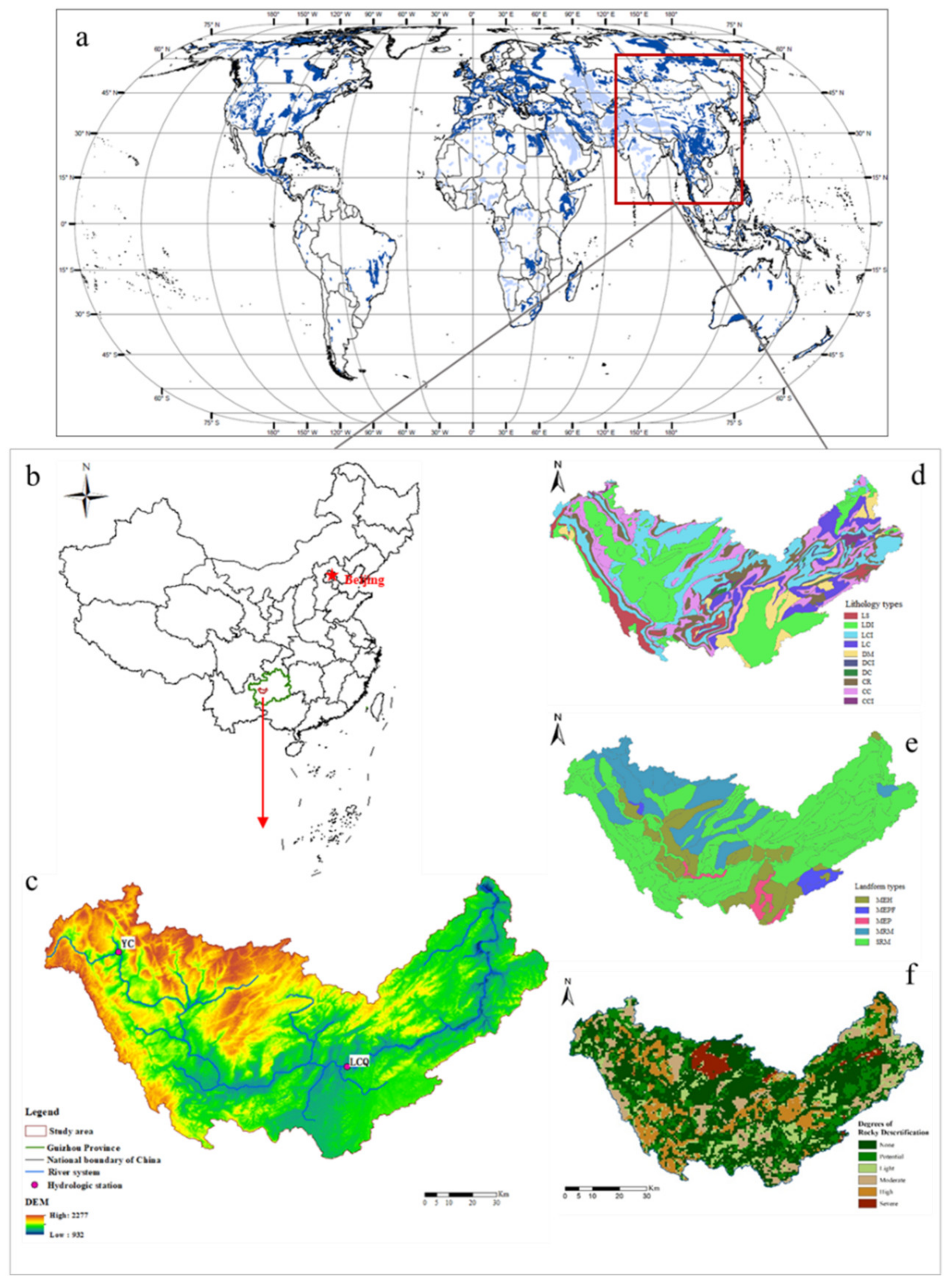
A typical karst peak-cluster depression area is selected in this study, located in the Guizhou Province of southwest China at 104°54′–106°24′E and 26°06′–27°00′N, with an area of 4861 km2. The study area lies in a subtropical monsoon climate zone, with a warm-humid climate and abundant rainfall. Heavy rains are concentrated between July and September. Karst geology, a binary hydrological structure, and thin and discontinuous soil are the typical environmental features of the study area [25,26]. Hydrological processes experience rapid changes, and the spatial distribution of water and soil resources do not correspond well [27]. The lithology types include limestone, dolomite, interbedded limestone and dolomite, limestone with clastic rocks, dolomite with clastic rocks, interbedded limestone and clastic rocks, interbedded dolomite and clastic rocks, clastic rocks, and clastic rocks with carbonate, among which limestone with clastic rocks LC and interbedded limestone and clastic rocks account for more than half of the study area (Table 1). Karst landforms mainly consist of middle elevation plains, middle elevation terraces, middle elevation hills, small relief mountains, and middle relief mountains (Table 1). In terms of the Hydrological yearbook of the People’s Republic of China—Wujiang area, Yangtze river basin, the tributary of Wujiang river runs through and there are two hydrological stations in this study area (YC and LQC, Figure 1c). Combined with DEM data of this area, the area near YC station is defined as upstream, the area near LQC station as middle stream, and the remaining area as the downstream. This division is convenient for subsequent description and analysis of spatial pattern. According to the rocky desertification data (http://www.forestry.gov.cn/), we found significant rocky desertification in this area. The grade of rocky desertification degree is divided according to the bare reate of bedrock (Table 2), referring to the classification criteria of Bai et al. [28], Li et al. [29], and Gao et al. [30]. In this study area, there are 55.3% of the area with potential, light, moderate, high and severe rocky desertification. The area percentages, respectively, are 17.2%, 9.80%, 13.00%, 12.3%, and 3.00% (Figure 1f).
2.2. Datasets
2.2.1. Land Use Data
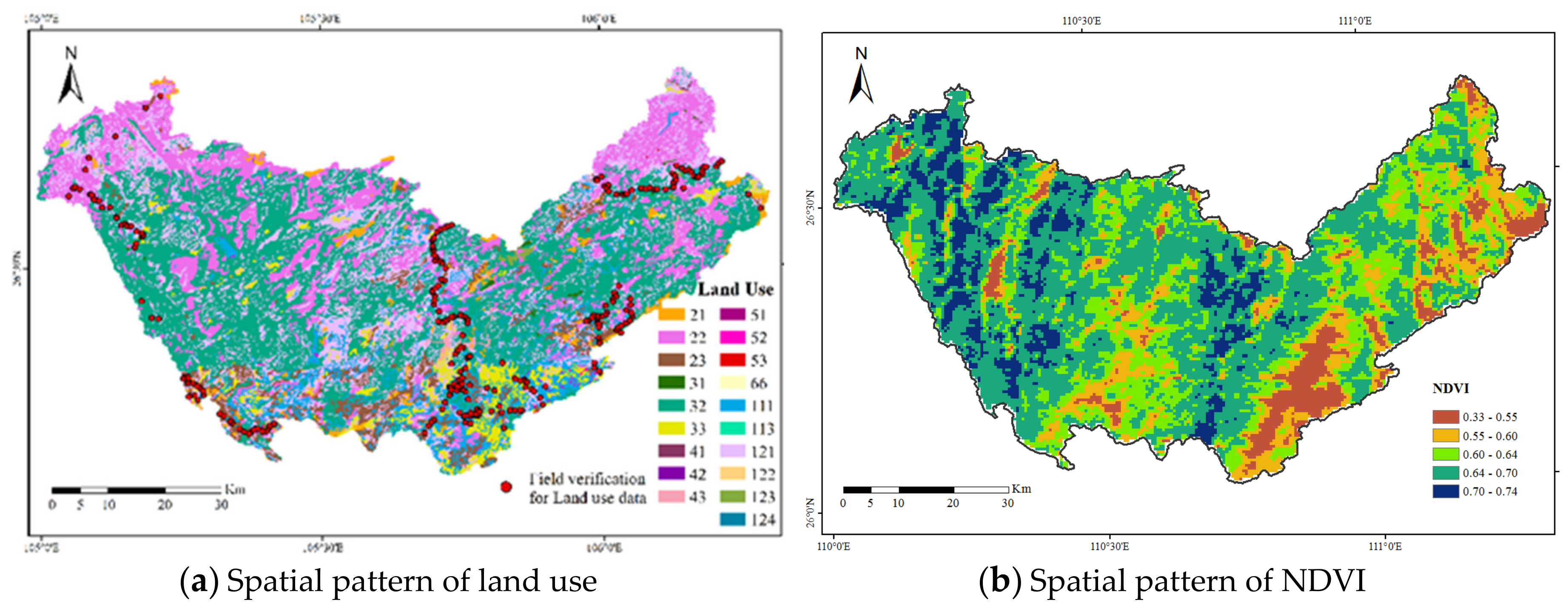
The land use data set was provided by the Data Center for Resources and Environmental Sciences, Chinese Academy of Sciences (RESDC) (http://www.resdc.cn), which was interpreted from 30 m-resolution Landsat TM images by supervised classification methods, based on field sampling points (Figure 2a) collected by GPS with ENVI software. The efficient of Kappa was 0.81 through the mode of Classifier-Accuracy Assessment in Erdas, which meant the remote sensing data of land use was reliable. The region includes seven primary land use types: garden plot, woodland, grassland, commercial land, industrial and warehouse land, water areas, and other land. The dominant types are woodland and garden plot, occupying 43.6% and 26.2% of the region, respectively. Commercial and service land, and industrial and warehouse land occupies a small area, mainly in the southeast. Water conservation and facility land only accounts for 7.9% of the region, and other land use types are scattered throughout the whole region. Approximately 20 secondary land use types exist (Figure 2a), which were used to calculate the landscape fragmentation index.
2.2.2. MODIS NDVI Data
Vegetation activity can be indicated by NDVI [31], and also the conditions of vegetation cover and productivity in a lot of researches [13,32]. NDVI from Moderate Resolution Imaging Spectroradiometer (MODIS, http://ladsweb.nascom.nasa.gov/) dataset, provided by the EOS/Terra of National Aeronautics and Space Administration, was used to reflect vegetation activity [33]. Then, 500-m spatial resolution MODIS NDVI data were collected for the 2005 to 2010 period. This dataset was produced by maximum value composite (MVC) methods to reduce the impacts of atmospheric clouds, shadows, solar zenith angle, and aerosol scattering. Radiation correction and geometric rectification were also applied. It was first cropped for the study area, and then transformed to the Krasovsky_1940_Albers projection. The NDVI dataset was applied to detect the spatial relationship between landscape fragmentation and vegetation activity.
As shown in Figure 2b, NDVI values vary from 0.33 to 0.74, with an average of 0.64. Vegetation activity, represented by the annual mean NDVI from 2005 to 2010, declines from west to east in the study area. Spatial statistics show that areas with higher NDVI values (i.e., larger than the average) occupy 47% of the whole area, and areas with NDVI values below 0.5 only account for 9%. This indicates that vegetation activity is relatively strong, especially in the upstream area, which is mainly covered with forest and shrub land (Figure 2a). Lower NDVI values, or weaker vegetation activity, are widely distributed in downstream areas due to greater human disturbance, such as steep slope reclamation, heavy grazing, and urbanization.
2.3. Methods
2.3.1. Landscape Fragmentation Index
Effective mesh size (meff), as an index of landscape fragmentation, was used to directly reflect landscape patterns in this study [34]. Ecological processes, landscape composition, and spatial patterns were all considered in this index to more objectively and comprehensively express fragmentation level [35]. The meff is the average of the continuous distribution area of different land use types in the region. The lower the mesh value is, the greater the degree of landscape fragmentation. The formula is:
where meff (j) is the meff of landscape j, n is the number of unbroken pieces in landscape j, and Aij is the area of plaque i in landscape j. The meff ranges from grid size to the landscape area. The grid type differs from its neighbors, and there is only one type of landscape. The landscape analysis software FRAGSTATS [36] was used to calculate the meff value.
2.3.2. Geostatistical Method: Semi-Variance Function
Spatial heterogeneity is the main cause of landscape patterns [37,38], and the scale effect should be considered in the analysis of spatial heterogeneity [39]. So, a geostatistical method was applied to obtain the appropriate analysis scale. Geostatistics is based on the theory of regionalization variables, and it is used to analyze random and structured natural spatial patterns with semi-variograms. In this study, an overall analysis of the spatial variation in this region would be carried out with the methods of semi-variable function. This can be carried out by GS+ 7.0, which is a comprehensive geostatistics program that is fast, efficient and easy to use.
The meff variogram was computed as half the expected squared increment of the values between locations xi and xi+h:
where N(h) is the number of pairs within a given spatial distance (and direction) known as lag h, and Z(xi) and Z(xi+h) are values of the indicator variable at locations xi and xi+h, respectively.
The nugget C0, sill (C0+C), range, ratio between C0 and (C0+C), and determination coefficient can quantify the degree of spatial variability. C0, which is the intercept on the y-axis, accounts for uncorrelated spatial noise or for spatial structures not detected at the analysis scale, and reflects internal randomness. C represents the spatial heterogeneity of structural factors, such as climate and landforms. The sill is an indicator of the overall spatial variance of the data. C/(C0+C) is the ratio of spatial heterogeneity of structural factors to the total spatial heterogeneity, which reflects the influence of structural factors on total spatial heterogeneity [40]. The range (r) indicates the distance at which the variogram reaches its sill. Data separated by a distance larger than the range are uncorrelated.
2.3.3. Geographically Weighted Regression Model
GWR is an extension of traditional regression methods, whereby local rather than global parameters can be estimated [41]. It can address the issue of a spatial non-stationary process, in which the parameter estimates are functions of location [42]. The relative value of the regression coefficient represented the degree of correlation, and the local determination coefficient (R2), ranging from 0 to 1, indicated how well the local regression model fit the observations [43]. The model is run for an observation point, using a spatial kernel that focuses on that point, and weighs observations subject to a distance decay function.
The model is expressed as:
where yi, xik, and εi represent the dependent variable, the independent variable, and the random error term at location i, respectively. (μi, vi) denotes the coordinate location of the ith point, k is the independent variable number. β0(μi, vi) expresses the intercept, and βk(μi, vi) is the slope coefficient for xk at location i.
The parameters are estimated from:
where β(μi, vi) is the unbiased estimate of the regression coefficient, W(μi, vi) represents the weighting matrix. X and Y are matrices for independent and dependent variables, respectively.
The weighting function (kernel function), can be calculated by the exponential distance decay form, Gauss function:
where ωij is the weight of observation j for location i, dij represents the Euclidean distance between points i and j, and b is the kernel bandwidth. If observation j coincides with i, the weight value is 1, while wij is decreasing according to a Gaussian curve as the distance dij increases. The optimal bandwidth ensures that macro patterns are accurate and local information is distinct. Bandwidth is one of the most important parameters in this regression model, which is a nonnegative attenuation parameter describing the functional relationship between weight and distance. The larger the bandwidth, the slower the weight decays with distance. According to the theory of the model, AICc (revised Akaike information criteria) value is the primary criteria for determining bandwidth. If the AICc values of the two models differ by more than 3, the model with lower AICc values will be considered as the better model.
2.3.4. Research Procedures
Based on land use data, landscape patterns and spatial variability were studied, and the spatial correlation between meff and NDVI was analyzed using the following steps: (1) The degree of landscape fragmentation was calculated by FRAGSTATS according to the size of the “sliding window”, employing 30-m resolution land use data. (2) GS+ 7.0 was used to calculate the spatial heterogeneity for different analysis scales (250 m, 500 m, 1500 m. etc.) and to determine the appropriate landscape size. (3) Multi-scale analysis was carried out with the size of “sliding window” as the abscissa and the value of spatial variability under the corresponding size as the ordinate. (4) Based on the multi-scale analysis (i.e., multiple neighborhood sizes), the feature points of scale transformation are revealed and regarded as sliding window size suitable for describing landscape fragmentation in this study area. (5) Landscape fragmentation index was calculated based on the analysis size, and GWR were applied to explore the relationship between landscape fragmentation and vegetation activity.
3. Results and Analysis
3.1. Spatial Heterogeneity of Landscape Fragmentation
3.1.1. Scale Dependence of Landscape Fragmentation
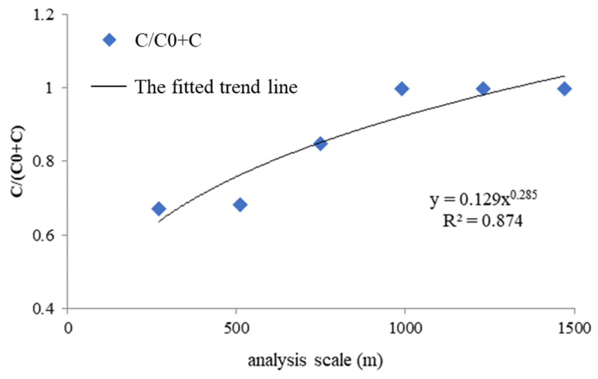
Landscape patterns are spatially correlated and scale-dependent [17]. The spatial variation of landscape fragmentation differs from the scale variation, so an accurate analysis scale is crucial for studying landscape patterns. Figure 3 shows the variation degree of spatial heterogeneity in landscape fragmentation at different analysis scales, which reflects the spatial heterogeneity of structural factors. A higher ratio indicates a stronger degree of spatial autocorrelation or a weaker degree of spatial variation. The scale analysis of landscape fragmentation in the study area indicates a power law relationship between effective mesh size and analysis scale (Figure 3). As shown in the Figure 3 of the manuscript, the spatial differences controlled by the structural factors decrease gradually with the analysis size changing from 1500 m to 250 m. It starts to stabilize at 500 m. On the other hand, the spatial differences controlled by random factors also tends to be stable. Therefore, it is reasonable and accurate to analyze the spatial difference under the analysis scale of 500 m. Furthermore, R2, which represented the fitting effect, also reached 0.98. According to this experts’ advice, the C/(C0+C) of 250 m is similar to 500 m, but a larger analysis scale of 500 m revealed sufficient spatial heterogeneity information, and thus optimally reflected the intrinsic spatial heterogeneity scale of landscape fragmentation. Therefore, an analysis scale of 500 m was chosen to calculate the landscape fragmentation. Meanwhile, in order to keep the same scale with the landscape fragmentation, the NDVI product should also be 500 m, so as to finally study the impact of landscape pattern on vegetation activities.
3.1.2. Spatial Distribution of Landscape Fragmentation
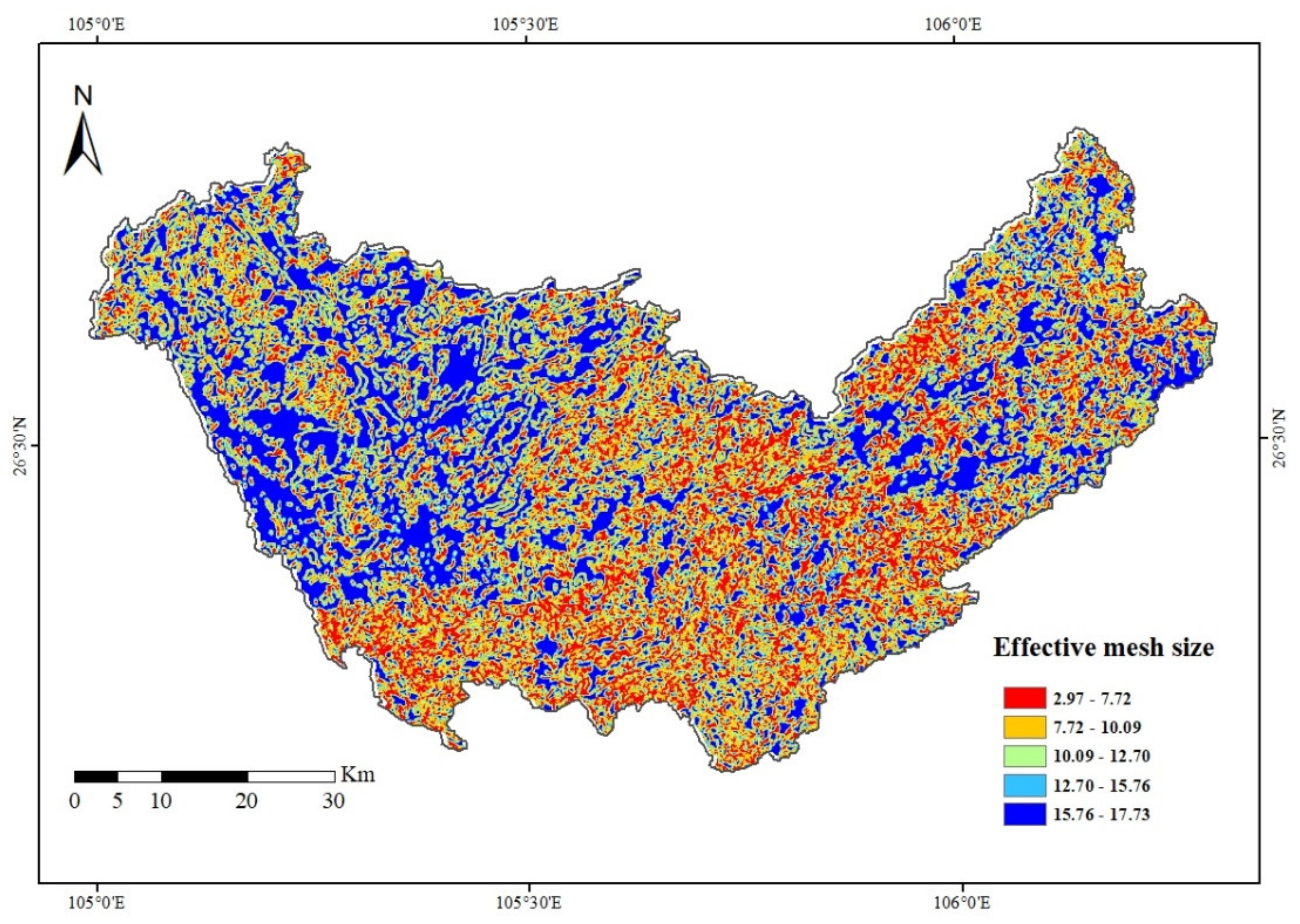
From an overall perspective, the study area shows a different distribution of high and low meff values, with a larger area of low meff values (Figure 4). Low meff values are mostly located in the middle and lower streams of the study area, where the degree of landscape fragmentation is more serious. In upstream areas, with high elevation and weaker human disturbance, there is less landscape fragmentation. According to different land use types, the meff values of forest land are mostly high, with an average of 12.13, which is greater than the mean of the whole region (11.70). This may be due to the concentrated and broad distribution of forest land, resulting in weaker landscape fragmentation compared to other land use types. The values of the other four land use types are mostly below average.
At the same time, we further analyzed the spatial heterogeneity of this area based on semi-variance function (Table 2), and exponential model was used to simulate spatial variance of meff, showing good fitting effect, with R2 reaching 98.4%. Results indicate that the influences of random factors are relatively weak, and account for 31.8% of the total impacts, and structural factors are dominant (C = 68.2%). The degree of landscape fragmentation is high in the middle stream of the study area, and is distributed on forest land, garden land, watershed, grass land, commercial services land, and other land use types. Furthermore, human activity is substantially higher in the middle stream. It is concluded that the landscape pattern distribution is mainly impacted by the structural factors in the study area, including unique geological conditions and highly fluctuating landforms, while the random factors such as local climate factors and human activities have little influence.
3.1.3. Variation Characteristics of Landscape Fragmentation under Different Environmental Factors
Compared with other regions, the degree of landscape fragmentation is greater in this study area, with an average meff value of 11.70. For example, in the urban fringe of Shunyi district in Beijing, the average was 42.45, with a range of 7.2–98.01 [44], despite intense human activities. This may be related to the special geological and geomorphological conditions, which led to landscape fragmentation. Therefore, elevation, slope, lithology, and landforms were considered in the impact analysis of landscape fragmentation, which paves the way for subsequent analysis of spatial relationship between landscape fragmentation and NDVI.
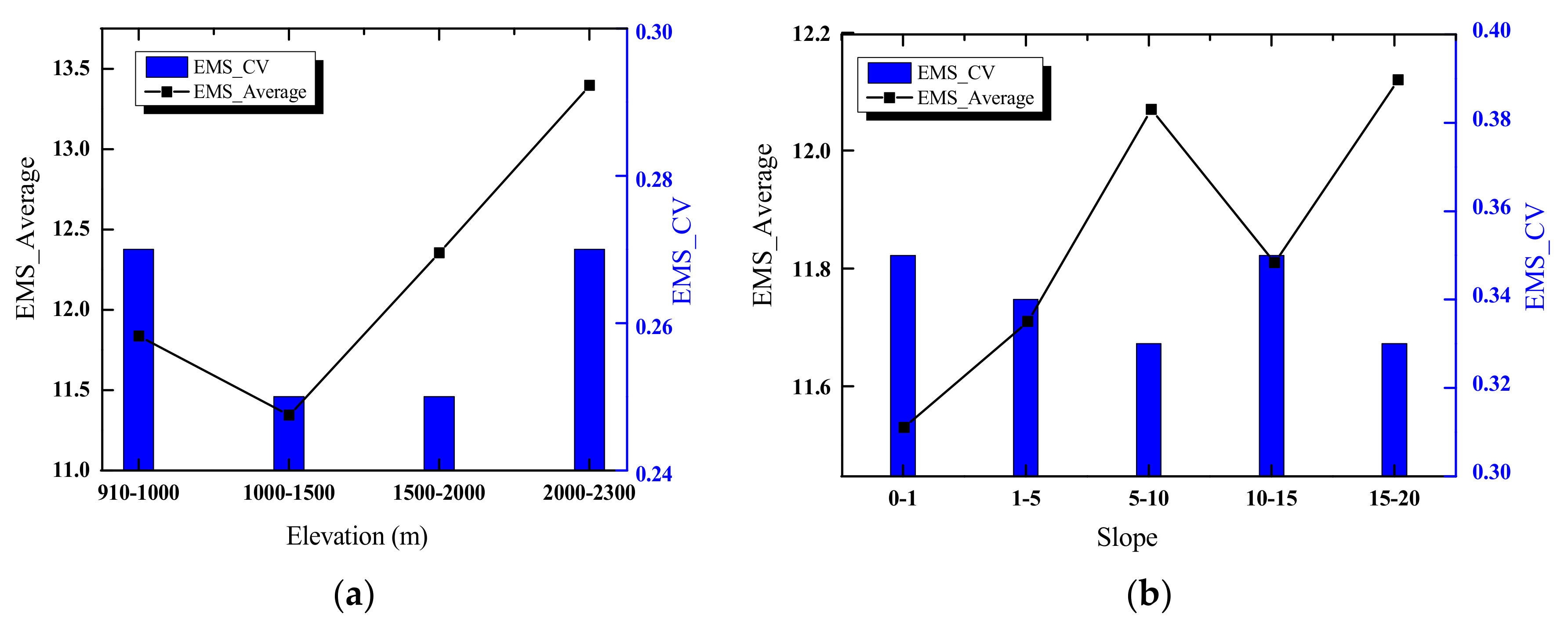
Elevation and slope are the basic topographic factor. So the basic law of landscape fragmentation with their changes should be preliminarily understood, as the analysis background of lithology and landform conditions. It is found (Figure 5) that meff values increase with elevation, with the greatest fragmentation in the range of 1000–1500 m, the weakest fragmentation in the range of 2000–2300 m. However, the meff values fluctuate with the increase in slope, and there is no obvious upward or downward trend. Variations in meff value at different elevation and slope are both not evident.
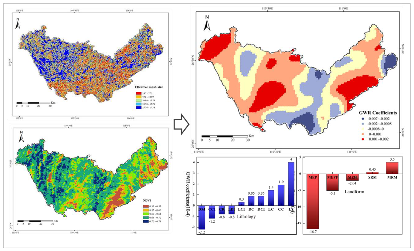
The results (Table 3) of the statistical analysis on the landscape fragmentation of different lithology types suggest that a high fragmentation degree for continuous and intercalated carbonate lithologies (i.e., LS, DM, LC, DC) was at a high level, and the type of rock alternating (i.e., LCI, DCI) was low. It can be deduced that the degree of fragmentation is more serious in carbonate than non-carbonate rocks, and that the higher the content of carbonate, the more serious the fragmentation, which may be due to strong karst erosion in the carbonate region. For dolomite lithologies, the order of meff values is DM<DC<DCI (Table 3), indicating that fragmentation degree gradually increases as the content of clastic rock decreases. Areas of dolomite with clastic rocks occur in regions of high elevation and steep slopes (middle relief mountain), which result in a fragmented landscape, but limestone regions are found in small relief mountains. The same pattern is not found in limestone rocks (i.e., LCI>LS>LC), in that fragmentation degree first increases then decreases with increasing clastic rock content. In addition, the fragmentation degree differs according to landform type, which combines elevation, slope, and terrain (e.g. plain, hill). The degree of fragmentation is most serious for middle elevation plains, and follows the order: middle elevation terrace>middle elevation hill>small relief mountain>middle relief mountain, with meff values from 10.59 to 12.47.
3.2. Spatial Relationship Between Landscape Fragmentation and Vegetation Activity Based on GWR Model
3.2.1. Multi-scale Simulation Using GWR Model
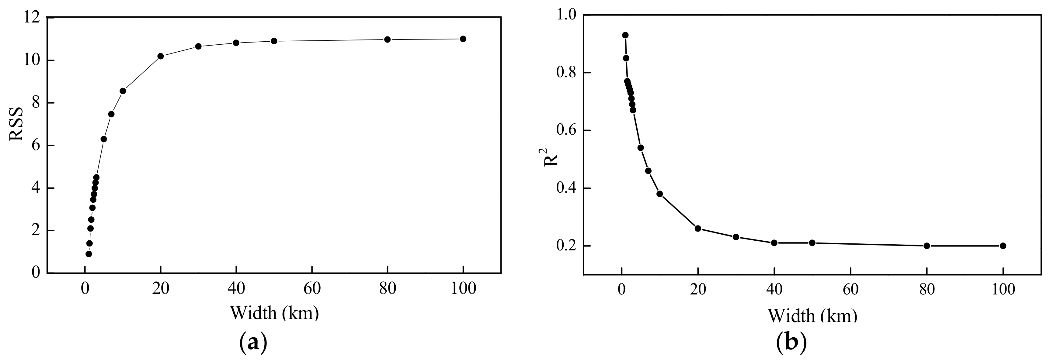
GWR was used to analyze the spatial relationship between landscape pattern and vegetation activity, and bandwidth (the analysis scale of correlation research) can impact the simulation effect of regression. To ensure that GWR effectively describes the non-stationary spatial correlation, an optimal bandwidth should be selected. Here, comprehensively considering the confirmed standard of bandwidth and the actual meaning of weight function, a bandwidth of 7 km was selected as the analysis scale for this GWR model in this study. The process is as follows.
An AICc value of 7 km is the smallest through model calculation, but the differences of AICc values between 7km and 4 km, 5 km, 6 km, respectively, are less than 3. However, residual sum of squares (RSS) and the coefficient of determination (R2) values of scales less than 7km seem to have a good fitting effect, with low RSS and high R2 (Figure 6). Under this circumstance, the functional relationship between bandwidth and weight is also considered. According to the Gaussian function, the smaller the bandwidth, the greater the reduction in weight with the increase in unit distance, which is similar to the inverse distance weight model. Apparently, this is inconsistent with the original intention of the GWR model. Furthermore, Figure 6 shows that the value changes of different scales gradually leveled off from 7 km, and the R2 was 0.46 at a bandwidth of 7 km. Taking the above reasons into consideration, the scale of 7 km can not only meet the requirement of having a smaller AICc value, meaning a better fitting effect, but also represents the macro pattern of the region accurately and depicts the local information clearly.
3.2.2. Spatially Relationships Between Landscape Fragmentation and Vegetation Activity
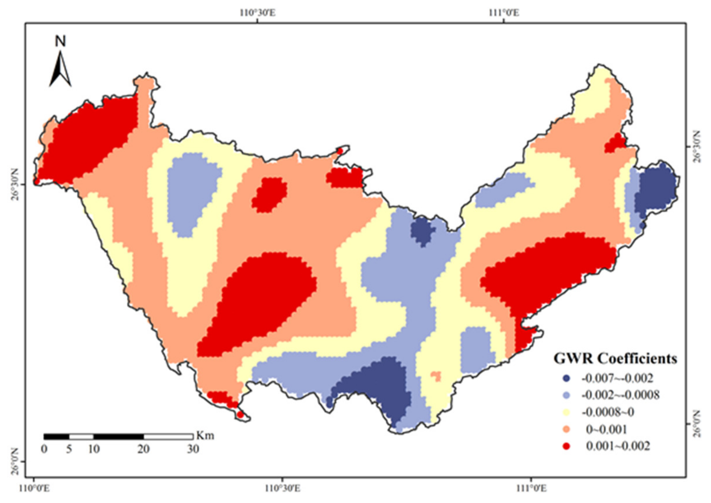
Due to its advantage of regional parameter estimation, the GWR model was used to quantify the spatial correlation between landscape fragmentation and vegetation activity, with R2 being 0.46. Considering that the prerequisite of the GWR method’s application is the spatial difference between the independent and dependent variables—that is, the regression coefficients change with the spatial position of independent variables [44] —this study conducted spatial autocorrelation analysis on the regression coefficient. The spatial autocorrelation index of regression coefficients is 0.84, calculated by the Spatial Statistics Tools—Spatial Autocorrelation mode of ArcGIS, which indicates that the coefficients are non-stationary spatially. The Z value is more than 2.58 times standard deviation, which is statistically significant at the significant level of 0.01.
The regression coefficients are clearly spatially heterogeneous (Figure 7). Positive and negative correlations are distributed throughout the study area. Negative correlations between NDVI and meff are mainly distributed in the northeast, and account for 45.4% of the whole region. Positive relationships are mostly located in the east and west. In the upstream of the study area, the relationship between NDVI and meff is predominantly positive. This can be attributed to the low degree of landscape fragmentation in the upstream, which is mainly shrub and orchard land, and where vegetation cover is in a good condition. In the middle stream, both positive and negative correlations are found. This area shows high landscape fragmentation, and high NDVI may be influenced by temperature, precipitation and terrain, among other factors. Downstream areas mainly show positive correlations. That is, the more fragmented the landscape is, the lower the NDVI value. This also indicates that human activities, such as uncontrolled exploitation and utilization of natural resources, have an important effect on vegetation. Particularly in the southeast, the absolute value of the regression coefficients is significantly larger on commercial services land and industrial warehouse land.
3.3. Effect of Environmental Factors on the Spatial Relationship Between Landscape Fragmentation and Vegetation Activity
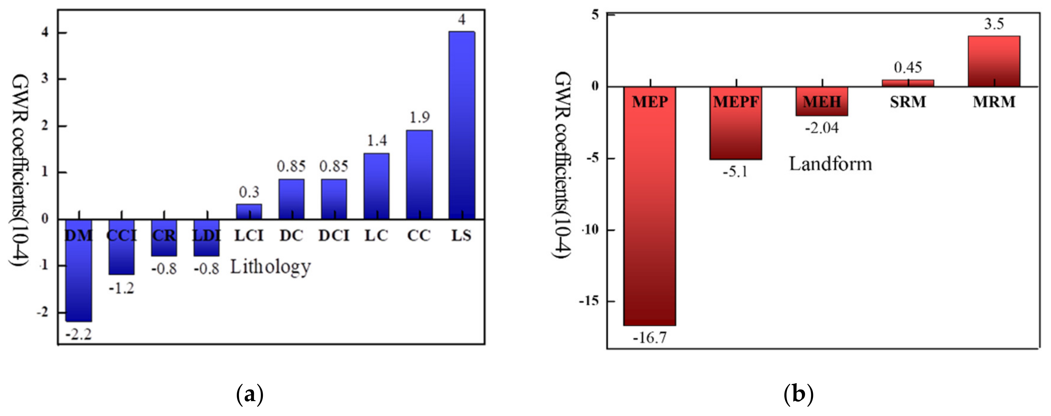
The relationship between landscape patterns and vegetation activity shows significant spatial heterogeneity. Lithology is an important and intrinsic factor of karst regions, which influences the formation of landscape patterns and ecosystem function. The GWR coefficients of different lithology types are analyzed statistically. Results show that the coefficients are positive in areas of limestone and limestone mixed with clastic rocks, at 4 × 10⁻⁴ and 1.4 × 10⁻⁴, respectively, and those in continuous dolomite (DM) areas are negative (−2.2 × 10⁻⁴). In limestone (LS) areas, the greater the degree of landscape fragmentation, the poorer the vegetation activity. This rule becomes weaker as the content of clastic rocks increases. Relatively higher correlations also indicate that ecological functions are more sensitive to changes in the external environment. In contrast, the average GWR coefficient in DM regions (meff = 11.10) is negative; the more severe the landscape fragmentation, the better the vegetation activity. The terrain in DM regions is typically gentle, and may be affected by human activities, including afforestation and grain for green in this area. In addition, statistical results (Table 4) show that the GWR coefficient fluctuates with elevation and slope with no clear trend.
A clearer effect of elevation and slope is observed for different landform types (Figure 8). For example, negative relationships between landscape fragmentation and vegetation activity are found in middle elevation hills, middle elevation terraces, and middle elevation plains. A positive correlation occurs in small relief and middle relief mountains. In middle relief mountains, the positive relationship reflects weak human disturbance. In middle elevation regions, human activity has a more important impact on the relationship. Moreover, projects of rocky desertification management have led to improvement of the ecological environment, but may have also led to landscape fragmentation.
4. Discussion
This research, guided by the relationship between geographical structure and function, systematically explores the spatial relationship between landscape pattern and ecological function. A set of methodological frameworks suitable for this region was constructed, through studying spatial relationship between them. The regional rules obtained from this framework will provide scientific support for the spatial optimization and treatment of rocky desertification areas.
The degree of landscape fragmentation is influenced by environmental factors (elevation, slope, lithology and landform), both directly and indirectly. Carbonate lithology and terrain with higher relief are typically more prone to landscape fragmentation. However, add to the effect of human activities, the spatial distribution of landscape fragmentation is highly complex. Furthermore, this study also found that the fragmentation degree and its relationship with vegetation activities showed obvious differences in the different lithology types of karst areas. Specifically, landscape fragmentation in DM regions is significantly higher than in LS, LCI, DCI, and DC regions, where the terrain is steeper. In flat areas, human activities are more intense, which enhances fragmentation. However, the ecological function of the area with serious fragmentation is better, and we think this may be due to the ecosystem restoration projects in the flat DM region. For areas of limestone dominance, the influence of human activities is not greater than for the DM region. Due to the obviously positive relationship between landscape fragmentation and vegetation activities in these areas, we found that the ecological functions of landscape fragmentation are much more significant, and assume that they are more sensitive to the changes of external physical environment. Meanwhile, we also found some problems. The landscape fragmentation averages under different geological and topographic conditions (elevation, slope, lithology and landform) are concentrated on the range of 10.6–13.5, which is smaller than the range in the spatial pattern map of the whole study area, of 2.97–17.73. That is to say, under the same geological or topographic conditions, different levels of landscape fragmentation can be distributed with great differences, resulting in the lack of characteristic in the average value of the final landscape fragmentation degree under a certain condition. This phenomenon indicates that the fragmentation of region landscape is comprehensively affected by a variety of factors, with interactions between factors playing important roles. Therefore, it is necessary to analyze the interaction of different factors, which will be further studied in the future, in order to deeply understand the influencing mechanism of landscape fragmentation. In addition, there are some uncertainties in this study. For example, the possible impact of human activities is mentioned in the analysis of influence factors in this study, but the limited data mean it is not quantified. So, if the impact of human activities is represented by the corresponding human and economic parameters, the quantitative relationship between human activities and topographic conditions and vegetation activities can be accurately explored, which can further enhance the persuasiveness of the research results; we plan to do this in future research.
According to the above results of spatial pattern characteristics, it is found that this region does have high spatial heterogeneity. So, considering the uniqueness of this karst area, a multi-scale analysis should be conducted before calculating the meff and regression relationship, as is conducted in the study. Based on the multi-scale statistical relation analysis, significant power law relations between spatial variance and analysis scale, and exponential change rules between the determination coefficient of spatial relationship of fragmentation-vegetation activity and analysis scale, are identified, of which 500 m and 7 km are intended to be the regional characteristic scales of fragmentation calculation and relationship fitting, respectively.
Furthermore, the results of this study are of practical significance. For example, the meff value is mostly low in dolomite regions, but the relationship between mesh and NDVI suggests a beneficial effect of landscape fragmentation on vegetation activity. Thus, although ecological restoration can be seen to be harmful through landscape fragmentation, it can also enhance the ecological function and improve the ecological environment, which is the ultimate aim of landscape ecology research. These results can provide more objective, scientific, and comprehensive theoretical support, and, furthermore, provide guidance for ecological restoration.
5. Conclusions
The spatial relationship between landscape pattern and ecosystem process and function is complex, yet it is the key to ecosystem services research and ecological restoration. In this study, the spatial heterogeneity of landscape fragmentation and its spatially non-stationary relationship with vegetation activity was detected using geostatistical analysis and a GWR model for this study area. Moreover, a multi-scale analysis based on landscape size and GWR neighborhood size was conducted in view of spatial variability. Considering the impact of topography and lithology on land use and vegetation activity in mountainous karst areas, the influences of these factors were investigated.
Firstly, we found the spatial pattern of landscape fragmentation showed clear heterogeneity, which is mainly dominated by the structural factors (e.g., geology, topography, and other physical environmental factors). The fragmentation degree was mostly high in the region, with the range of 2.97–17.73 and the mean of the whole region being 11.70. Among them, the value of woodland is the largest, and the value is 12.13. Moreover, compared to non-carbonate regions, the degree of landscape fragmentation was greater in carbonate areas, with the smallest value of different lithology types being 10.95 in the LC area, as well as the DM areas. The influence of human activities on the morphological characteristics of dolomite regions was much more significant than that in limestone regions. Secondly, the spatial relationship between landscape fragmentation and vegetation activity was also highly heterogeneous, and negative correlations are mainly distributed in the northeast, accounting for 45.4% of the whole region. In limestone regions, larger coefficients, e.g., the largest of 4 × 10⁻⁴ in LS areas, revealed significant negative effects on ecosystem function due to structural changes, which also reflected the greater sensitivity and vulnerability of the ecosystem to environment variations. Contrastingly, the coefficient of DM areas is the smallest, −2.2 × 10⁻⁴, which shows that the fragmented landscape had a beneficial effect on ecosystem function in flat areas with dolomite. This indicates that although the degree of landscape fragmentation may be exacerbated by ecosystem restoration projects, it could also improve the conditions of vegetation cover. Through these works, a methodology of multi-scale analysis for this area is also formed at the same time, including the thought and method of analysis scale and bandwidth, which would be helpful to further improve the landscape pattern and ecological effect in the karst mountain area.
Landscape ecology research contributes toward an understanding of ecosystem services and how land management can enhance sustainability of ecosystem services in a changing landscape. We suggest that the principles of "scientific analysis, prominent focus, clear objectives" should be paid more attention in relation to karst ecological management and rocky desertification control. The surface relief characterized by landscape fragmentation, and the ecological function characterized by vegetation activity, as well as the regional differences of different lithology and geomorphic units, especially, will be the scientific basis for treating both the symptoms and root causes and structure–function collaborative management of rocky desertification in the future, which is also the key for land management and urban planning. It is also an important impetus for ecological restoration and construction in this area, and provides a representative case for landscape ecology research, further contributing to the in-depth development of landscape ecology research.
Author Contributions
Conceptualization methodology, software, validation, investigation, writing—review and editing, and so on, were finished by W.H. and J.G. All authors have read and agreed to the published version of the manuscript.
Funding
This material is based upon work supported by the National Natural Science Foundation of China (No. 41671098, 41807168), and the National Key R&D Program of China (2018YFC1508900, 2018YFC1508801).
Acknowledgments
All the authors thank the Data Center for Resources and Environmental Sciences, Chinese Academy of Sciences (RESDC) and EOS/Terra of National Aeronautics and Space Administration, for producing and sharing the land use and NDVI dataset, respectively.
Conflicts of Interest
The authors declare no conflict of interest.
References
- Fu, B.; Li, S.; Yu, X.; Yang, P.; Yu, G.; Feng, R.; Zhuang, X. Chinese ecosystem research network: Progress and perspectives. Ecol. Complex. 2010, 7, 225–233. [Google Scholar] [CrossRef]
- Shen, Z.; Wang, Y.; Fu, B. Corridors and Networks in Landscape: Structure, Functions and Ecological Effects. Chinese Geogr. Sci. 2014, 24, 1–4. [Google Scholar] [CrossRef] [Green Version]
- Zhang, Q.; Wu, J. Research advances in the relationship between functional diversity and ecosystem function. In Lectures in Modern Ecology (VIII): Advances in Community, Ecosystem and Landscape Ecology; Gao, Y., Wu, J., Eds.; Higher Education Press: Beijing, China, 2017. [Google Scholar]
- Turner, B.; Meyer, W.; Skole, D. Global Land-Use/Land-Cover Change: Towards an Integrated Study. Ambio 1994, 23, 91–95. [Google Scholar]
- Fu, Y.; Lu, X.; Zhao, Y.; Zeng, X.; Xia, L. Assessment Impacts of Weather and Land Use/Land Cover (LULC) Change on Urban Vegetation Net Primary Productivity (NPP): A Case Study in Guangzhou, China. Remote Sens. 2013, 5, 4125–4144. [Google Scholar] [CrossRef] [Green Version]
- Fierro, P.; Bertrán, C.; Tapia, J.; Peña-Cortés, F.; Vergarab, C.; Cerna, C.; Vargas-Chacoff, L. Effects of local land-use on riparian vegetation, water quality, and the functional organization of macroinvertebrate assemblages. Sci. Total Environ. 2017, 609, 724–734. [Google Scholar] [CrossRef]
- Lu, X.; Zhou, Y.; Hou, X.; Li, J.; Liu, Y.; Zhang, Y. Vegetation change based on land use/cover in arid oasis: A case study of the Eighth Division of Xinjiang Production and Construction Corps. Chin. J. Eco-Agre. 2015, 23, 246–256. [Google Scholar]
- Dong, G.; Bai, J.; Yang, S.; Wu, L.; Cai, M.; Zhang, Y.; Luo, Y.; Wang, Z. The impact of land use and land cover change on net primary productivity on China’s Sanjiang Plain. Environ. Earth Sci. 2015, 74, 2907–2917. [Google Scholar] [CrossRef]
- Wu, J.; Shen, W.; Sun, W.; Tueller, T. Empirical patterns of the effects of changing scale on landscape metrics. Landsc. Ecol. 2002, 17, 761–782. [Google Scholar] [CrossRef]
- Hernández, Á.; Arellano, E.; Morales-Moraga, D.; Miranda, M. Understanding the effect of three decades of land use change on soil quality and biomass productivity in a Mediterranean landscape in Chile. Catena 2016, 140, 195–204. [Google Scholar] [CrossRef]
- Jocque, M.; Field, R.; Brendonck, L.; De Meester, L. Climatic control of dispersal-ecological specialization trade-offs: A metacommunity process at the heart of the latitudinal diversity gradient? Glob. Ecol. Biogeogr. 2010, 19, 244–252. [Google Scholar] [CrossRef]
- Gao, J.; Jiao, K.; Wu, S.; Ma, D.; Zhao, D.; Yin, Y.; Dai, E. Past and future effects of climate change on spatially heterogeneous vegetation activity in China. Earth’s Future 2017, 5, 679–692. [Google Scholar] [CrossRef] [Green Version]
- Andrew, R.; Guan, H.; Batelaan, O. Large-scale vegetation responses to terrestrial moisture storage changes. Hydrol. Earth Syst. Sci. 2017, 21, 4469–4478. [Google Scholar] [CrossRef] [Green Version]
- Piao, S.; Fang, J. Seasonal changes in vegetation activity in response to climate changes in China between 1982 and1999. Acta Geogr. Sin. 2003, 58, 119–125. [Google Scholar]
- Fang, J.; Piao, S.; He, J.; Ma, W. Increasing terrestrial vegetation activity in China, 1 during the last 20 years. Sci. China Ser. C 2004, 47, 229–240. [Google Scholar]
- Zheng, D.; Wallin, D.; Hao, Z. Rates and patterns of landscape change between 1972 and 1988 in the Changbai Mountain area of China and North Korea. Landsc. Ecol. 1997, 12, 241–254. [Google Scholar] [CrossRef]
- Wu, J. Effects of changing scale on landscape pattern analysis: Scaling relations. Landsc. Ecol. 2004, 19, 125–138. [Google Scholar] [CrossRef]
- Maciejewski, K.; Cumming, G. Multi-scale network analysis shows scale-dependency of significance of individual protected areas for connectivity. Landsc. Ecol. 2016, 31, 761–774. [Google Scholar] [CrossRef]
- Grêtregamey, A.; Rabe, S.; Crespo, R.; Crespo, R.; Lautenbach, S.; Ryffel, A. On the importance of non-linear relationships between landscape patterns and the sustainable provision of ecosystem services. Landsc. Ecol. 2014, 29, 201–212. [Google Scholar] [CrossRef]
- Hao, R.; Yu, D.; Liu, Y.P.; Liu, Y.; Qiao, J.; Wang, X.; Du, J. Impacts of changes in climate and landscape pattern on ecosystem services. Sci. Total Environ. 2016, 579, 718–728. [Google Scholar] [CrossRef]
- Garrigues, S.; Allard, D.; Baret, F.; Morisette, J. Multivariate quantification of landscape spatial heterogeneity using variogram models. Remote Sens. Environ. 2008, 112, 216–230. [Google Scholar] [CrossRef]
- Ungaro, F.; Zasada, I.; Piorr, A. Mapping landscape services, spatial synergies and trade-offs. A case study using variogram models and geostatistical simulations in an agrarian landscape in North-East Germany. Ecol. Indic. 2014, 46, 367–378. [Google Scholar] [CrossRef]
- Gao, J.; Li, S. Detecting spatially non-stationary and scale-dependent relationships between urban landscape fragmentation and related factors using Geographically Weighted Regression. App. Geogr. 2011, 31, 292–302. [Google Scholar] [CrossRef]
- Yu, Y.; Li, J.; Zhang, J. Effects of topography on land use pattern in Karst areas. In Proceedings of the International Conference on Environmental Science and Information Application Technology, Wuhan, China, 17–18 July 2010; pp. 760–763. [Google Scholar]
- Yuan, D. On the Karst environmental system. Carsologica Sin. 1988, 7, 179–186. [Google Scholar]
- Zhang, Z.; Chen, X.; Huang, Y.; Zhang, Y. Effect of catchment properties on runoff coefficient in a karst area of southwest China. Hydrol. Process. 2014, 28, 3691–3702. [Google Scholar] [CrossRef]
- Wang, S.; Li, R.; Sun, C.; Zhang, D.; Li, F.; Zhou, D.; Xiong, K.; Zhou, Z. How types of carbonate rock assemblages constrain the distribution of karst rocky desertified land in Guizhou Province, PR China: Phenomena and mechanisms. Land Degrad. Dev. 2004, 15, 123–131. [Google Scholar] [CrossRef]
- Bai, X.; Wang, S.; Chen, Q.; Cheng, A.; Ni, X. Spatio-temporal evolution process and its evaluation methods of karst rocky desertification in Guizhou Province. Acta Geogr. Sinica. 2009, 64, 609–618. [Google Scholar]
- Li, Y.; Bai, X.; Zhou, G.; Lan, A.; Long, J.; An, Y.; Mei, Z. The relationship of land use with karst rocky desertification in a typical karst area, China. Acta Geogr. Sin. 2006, 61, 624–632. [Google Scholar]
- Gao, J.; Wang, H. Temporal analysis on quantitative attribution of karst soil erosion: A case study of a peak-cluster depression basin in Southwest China. Catena 2019, 172, 369–377. [Google Scholar] [CrossRef]
- Fang, J.; Tang, Y.; Song, Y. Why are East Asian ecosystems important for carbon cycle research? Sci. China Life Sci. 2010, 53, 753–756. [Google Scholar] [CrossRef]
- Duo, A.; Zhao, W.; Qu, X.; Jing, R.; Xiong, K. Spatio-temporal variation of vegetation coverage and its response to climate change in North China plain in the last 33 years. Int. J. Appl. Earth Obs. Geoinf. 2016, 53, 103–117. [Google Scholar]
- Fang, J.; Piao, S.; Zhou, L.; He, J.; Wei, F.; Myneni, R.; Tucker, C.J.; Kun, T. Precipitation patterns alter growth of temperate vegetation. Geophys. Res. Lett. 2005, 322, 365–370. [Google Scholar] [CrossRef] [Green Version]
- Jaeger, J. Landscape division splitting index and effective mesh size new measures of landscape fragmentation. Landsc. Ecol. 2000, 15, 115–130. [Google Scholar] [CrossRef]
- Gao, J.; Cai, Y. Spatial heterogeneity of landscape fragmentation at multi-scales: A case study in Wujiang river basin, Guizhou Province, China. Scientia Geogr. Sin. 2010, 30, 742–747. [Google Scholar]
- Mcgarigal, K.; Marks, B. FRAGSTATS: Spatial Analysis Program for Quantifying Landscape Structure. USDA Forest Service - General Technical Report PNW, 351, Portland. 1995. Available online: https://www.fs.fed.us/pnw/pubs/pnw_gtr351.pdf (accessed on 1 October 2019).
- Yue, W.; Xu, J.; Xu, L.; Tan, W.; Mei, A. Spatial variance characters of urban synthesis indices at different scales. Chinese J. Appl. Ecol. 2005, 16, 2053–2059. [Google Scholar]
- Wu, J. Landscape Ecology: Pattern, Process, Scale and Level; Higher Education Press: Beijing, China, 2007. [Google Scholar]
- Levin, S. The problem of pattern and scale in ecology: The Robert H. Macarthur award lecture. Ecology 1992, 73, 1943–1967. [Google Scholar] [CrossRef]
- Wang, Z. Geostatistics and its Application in the Ecology; Science Press: Beijing, China, 1999. [Google Scholar]
- Fotherigham, A.; Brusdon, C.; Charlton, M. Geographically Weighted Regression: The Analysis of Spatially Varying Relationships; John Wiley & Sons: West Sussex, UK, 2002. [Google Scholar]
- Li, Z.; Huffman, T.; McConkey, B.; Townley-Smith, L. Monitoring and modeling spatial and temporal patterns of grassland dynamics using time-series MODIS NDVI with climate and stocking data. Remote Sens. Environ. 2013, 138, 232–244. [Google Scholar] [CrossRef]
- Chao, L.; Zhang, K.; Li, Z.; Zhu, Y.; Wang, J.; Yu, Z. Geographically weighted regression based methods for merging satellite and gauge precipitation. J. Hydrol. 2018, 558, 275–289. [Google Scholar] [CrossRef]
- Li, C.; Zhang, F.; Zhu, T.; Qu, Y. Analysis on spatial-temporal heterogeneities of landscape fragmentation in urban fringe area: A case study in Shunyi district of Beijing. Acta Ecol. Sin. 2013, 33, 5363–5374. [Google Scholar]
Figure 1.
Maps of world karst distribution (a) and basic environmental elements (d, lithology; e, landform; f, rocky desertification) for the study area(c) in the northwest Guizhou province of China (b).
Figure 1.
Maps of world karst distribution (a) and basic environmental elements (d, lithology; e, landform; f, rocky desertification) for the study area(c) in the northwest Guizhou province of China (b).

Figure 2.
Spatial patterns of land use (a) and vegetation activity (b) in the study area. Land use types are: 21 = orchard, 22 = tea garden, 23 = other garden, 31 = forest land, 32 = shrubland, 33 = other forest land, 41 = natural grassland, 42 = tame pasture, 43 = other grassland, 51 = wholesale and retail land, 52 = accommodation and catering land, 53 = commercial and financial land, 61 = industrial land, 62 = mining land, 63 = warehouse land, 66 = other lands, 111 = river surface, 113 = reservoir surface, 121 = vacant land, 122 = facility agricultural land, 123 = ridge , and 124 = saline-alkali land .

Figure 3.
Trends of spatial heterogeneity for landscape fragmentation at different scales.

Figure 4.
Spatial distribution of meff values (hm2) in the study area.

Figure 5.
Statistical analysis of the index of landscape fragmentation at different elevation (a) and slope (b).
Figure 5.
Statistical analysis of the index of landscape fragmentation at different elevation (a) and slope (b).

Figure 6.
Residuals (a) and R2 (b) of GWR models for different bandwidth scales.

Figure 7.
Spatial distribution of regression coefficients from the GWR models for NDVI and effective mesh size.
Figure 7.
Spatial distribution of regression coefficients from the GWR models for NDVI and effective mesh size.

Figure 8.
Statistical analysis of GWR coefficients for different lithology (a) and landform (b) types.
Figure 8.
Statistical analysis of GWR coefficients for different lithology (a) and landform (b) types.


Table 1.
Proportion of different lithology and landform types in the study area.
| Description | Area(km2) | Areal Percentage | Abbreviation | |
|---|---|---|---|---|
| Lithology types | limestone with clastic rocks | 373.3 | 7.68% | LC |
| clastic rocks | 471.0 | 9.69% | CR | |
| dolomite | 316.5 | 6.51% | DM | |
| clastic rocks with carbonate | 846.8 | 17.42% | CC | |
| limestone | 231.4 | 4.76% | LS | |
| interbedded limestone and dolomite | 1370.8 | 28.20% | LDI | |
| interbedded limestone and clastic rocks | 1196.8 | 24.62% | LCI | |
| interbedded dolomite and clastic rocks | 34.5 | 0.71% | DCI | |
| dolomite with clastic rocks | 19.9 | 0.41% | DC | |
| Landform types | middle elevation plain | 98.2 | 2.02% | MEP |
| middle elevation platform | 92.4 | 1.90% | MET | |
| middle elevation hill | 721.3 | 14.84% | MEH | |
| small relief mountain | 3020.6 | 62.14% | SRM | |
| middle relief mountain | 928.5 | 19.10% | MRM | |
Table 2.
Summary of model and structural components of the semi-variance functions for effective mesh size.
Table 2.
Summary of model and structural components of the semi-variance functions for effective mesh size.
| Landscape Fragmentation | Nugget C0 | Sill C0+C | C0/(C0+C) | Range (a/km) | Fractal | R2 | RSS | Fit Model |
|---|---|---|---|---|---|---|---|---|
| meff | 0.317 | 0.998 | 0.318 | 870 | 1.964 | 0.984 | 0.0016 | exponential model |
Table 3.
Statistical analysis of the index of landscape fragmentation by lithology and landform type.
Table 3.
Statistical analysis of the index of landscape fragmentation by lithology and landform type.
| Lithology and Landform | Average meff Value | Coefficient of Variance | |
|---|---|---|---|
| Lithology | limestone with clastic rocks (LC) | 10.95 | 0.345 |
| clastic rocks (CR) | 11.08 | 0.350 | |
| dolomite (DM) | 11.10 | 0.349 | |
| clastic rocks with carbonate (CC) | 11.55 | 0.342 | |
| limestone (LS) | 11.75 | 0.354 | |
| interbedded limestone and dolomite (LDI) | 11.97 | 0.331 | |
| interbedded limestone and clastic rocks (LCI) | 12.09 | 0.335 | |
| interbedded dolomite and clastic (DCI) | 12.33 | 0.325 | |
| dolomite with clastic rocks (DC) | 11.71 | 0.354 | |
| Landform | middle elevation plain (MEP) | 10.59 | 0.345 |
| middle elevation terrace (MET) | 11.04 | 0.330 | |
| middle elevation hill (MEH) | 11.30 | 0.342 | |
| Small relief mountain (SRM) | 11.61 | 0.345 | |
| middle relief mountain (MRM) | 12.47 | 0.317 | |
Table 4.
Statistical analysis of GWR coefficients for different elevation and slope.
| Elevation (m) | GWR Coefficients | Slope (°) | GWR Coefficients |
|---|---|---|---|
| 910–1000 | −5.7 × 10⁻⁴ | 0–5 | −18.5 × 10⁻⁴ |
| 1000–1500 | −19.6 × 10⁻⁴ | 5–10 | −10.8 × 10⁻⁴ |
| 1500–2000 | −5.6 × 10⁻⁴ | 10–15 | 1.3 × 10⁻⁴ |
| 2000–2300 | −13.4 × 10⁻⁴ | 15–20 | −14.1 × 10⁻⁴ |
© 2020 by the authors. Licensee MDPI, Basel, Switzerland. This article is an open access article distributed under the terms and conditions of the Creative Commons Attribution (CC BY) license (http://creativecommons.org/licenses/by/4.0/).
Share and Cite
MDPI and ACS Style
Hou, W.; Gao, J. Spatially Variable Relationships between Karst Landscape Pattern and Vegetation Activities. Remote Sens. 2020, 12, 1134. https://0-doi-org.brum.beds.ac.uk/10.3390/rs12071134
AMA Style
Hou W, Gao J. Spatially Variable Relationships between Karst Landscape Pattern and Vegetation Activities. Remote Sensing. 2020; 12(7):1134. https://0-doi-org.brum.beds.ac.uk/10.3390/rs12071134
Chicago/Turabian StyleHou, Wenjuan, and Jiangbo Gao. 2020. "Spatially Variable Relationships between Karst Landscape Pattern and Vegetation Activities" Remote Sensing 12, no. 7: 1134. https://0-doi-org.brum.beds.ac.uk/10.3390/rs12071134
Note that from the first issue of 2016, this journal uses article numbers instead of page numbers. See further details here.