ASTER Global Digital Elevation Model (GDEM) and ASTER Global Water Body Dataset (ASTWBD)

1
Jet Propulsion Laboratory, California Institute of Technology, Pasadena, CA 91109, USA
2
Sensor Information Laboratory Corp., Ibaraki 300-2359, Japan
*
Author to whom correspondence should be addressed.
†
Retired.
Remote Sens. 2020, 12(7), 1156; https://0-doi-org.brum.beds.ac.uk/10.3390/rs12071156
Submission received: 3 March 2020
/
Revised: 30 March 2020
/
Accepted: 2 April 2020
/
Published: 4 April 2020
(This article belongs to the Special Issue Advances in Global Digital Elevation Model Processing)
Abstract
:The Advanced Spaceborne Thermal Emission and Reflection Radiometer (ASTER) is a 14-channel imaging instrument operating on NASA’s Terra satellite since 1999. ASTER’s visible–near infrared (VNIR) instrument, with three bands and a 15 m Instantaneous field of view (IFOV), is accompanied by an additional band using a second, backward-looking telescope. Collecting along-track stereo pairs, the geometry produces a base-to-height ratio of 0.6. In August 2019, the ASTER Science Team released Version 3 of the global DEM (GDEM) based on stereo correlation of 1.8 million ASTER scenes. The DEM has 1 arc-second latitude and longitude postings (~30 m) and employed cloud masking to avoid cloud-contaminated pixels. Custom software was developed to reduce or eliminate artifacts found in earlier GDEM versions, and to fill holes due to the masking. Each 1×1 degree GDEM tile was manually inspected to verify the completeness of the anomaly removal, which was generally excellent except across some large ice sheets. The GDEM covers all of the Earth’s land surface from 83 degrees north to 83 degrees south latitude. This is a unique, global high spatial resolution digital elevation dataset available to all users at no cost. In addition, a second unique dataset was produced and released. The raster-based ASTER Global Water Body Dataset (ASTWBD) identifies the presence of permanent water bodies, and marks them as ocean, lake, or river. An accompanying DEM file indicates the elevation for each water pixel. To date, over 100 million 1×1 degree GDEM tiles have been distributed.
1. Introduction
A digital elevation model (DEM) is a digital raster representation of ground surface topography or terrain. Each raster cell (or pixel) has a value corresponding to its altitude above sea level. Topography is one of the primary attributes of the Earth’s surface. DEMs are used in numerous applications: extracting terrain parameters, modeling water flow, creation of relief maps, terrain analyses in geomorphology and physical geography, engineering and infrastructure design, base mapping, flight simulation, line of sight analysis, and many more. Morphometric data, such as slope, gradients, slope aspect, and hydrographic networks can be automatically extracted from DEMs. Hillshade images, curvature, contour lines, viewshed and observer points can also be calculated. In 2009, the US/Japan Advanced Spaceborne Thermal Emission and Reflection Radiometer (ASTER) project released the first global high spatial resolution digital elevation model (GDEM) available to all users. ASTER’s GDEM was created by stereo correlation of more than 1.2 million individual ASTER stereo scenes contained in the archive. The GDEM had 1 arc-second latitude and longitude postings (~30 m), and a vertical accuracy of approximately 10 m. The data were tiled as 22,000+ 1 × 1 degree latitude/longitude files, each accompanied by a quality file. The only other global high spatial resolution DEM in existence at the time was owned by the US National Geospatial Intelligence Agency (NGA), and remains classified to this day. In Version 2, released in 2011, the GDEM was improved, with reduction of artifacts, higher-resolution correlation, and additional scenes to fill in holes. In 2019, Version 3 was released. This final version of the GDEM was processed with new custom software to eliminate most artifacts, addition of 200,000 scenes to fill holes, and to improve infilling of the few holes remaining. The methodology used to produce the most recent GDEM is described in this contribution.
In addition to the improved GDEM Version 3, a second, unique dataset was created and released: the ASTER Global Water Body Dataset (ASTWBD). The ASTWBD is the only near-global raster dataset that delineates all water bodies smaller than 0.2 km2. The dataset defines the type of water body and identifies each water pixel as ocean, lake or river; an accompanying elevation file reports the elevation for each water pixel. The processing methodology is described below.
2. ASTER Instrument
The ASTER project is a joint endeavor by Japan’s Ministry of Economy, Trade and Industry (METI) and the U.S. National Aeronautics and Space Administration (NASA). METI provided the instrument; NASA provided the spacecraft and launch vehicle. The joint US/Japan ASTER Science Team is responsible for scheduling data acquisition, maintaining instrument calibration, and archiving and distributing data to users.
The ASTER instrument [1], launched onboard NASA’s Terra spacecraft in December 1999, is a 14-channel imaging instrument, with bands in visible–near infrared (VNIR), shortwave infrared, and thermal infrared. The VNIR sensor has an along-track stereoscopic capability using its near infrared spectral band to acquire the stereo data. The ASTER VNIR instrument has two telescopes—one for nadir viewing and another for backward viewing—with a base-to-height ratio of 0.6. The spatial resolution is 15 m in the horizontal plane. One scene consists of 4100 samples by 4200 lines that corresponds to approximately 60 by 60 km ground area. For almost every daytime image acquisition, ASTER captures a stereo pair. Currently, there are over 2.5 million stereo images in the archive.
3. ASTER Global Digital Elevation Model (GDEM) Version 3
3.1. Background: GDEM Versions 1 and 2
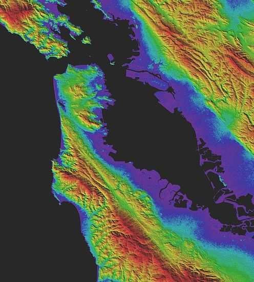
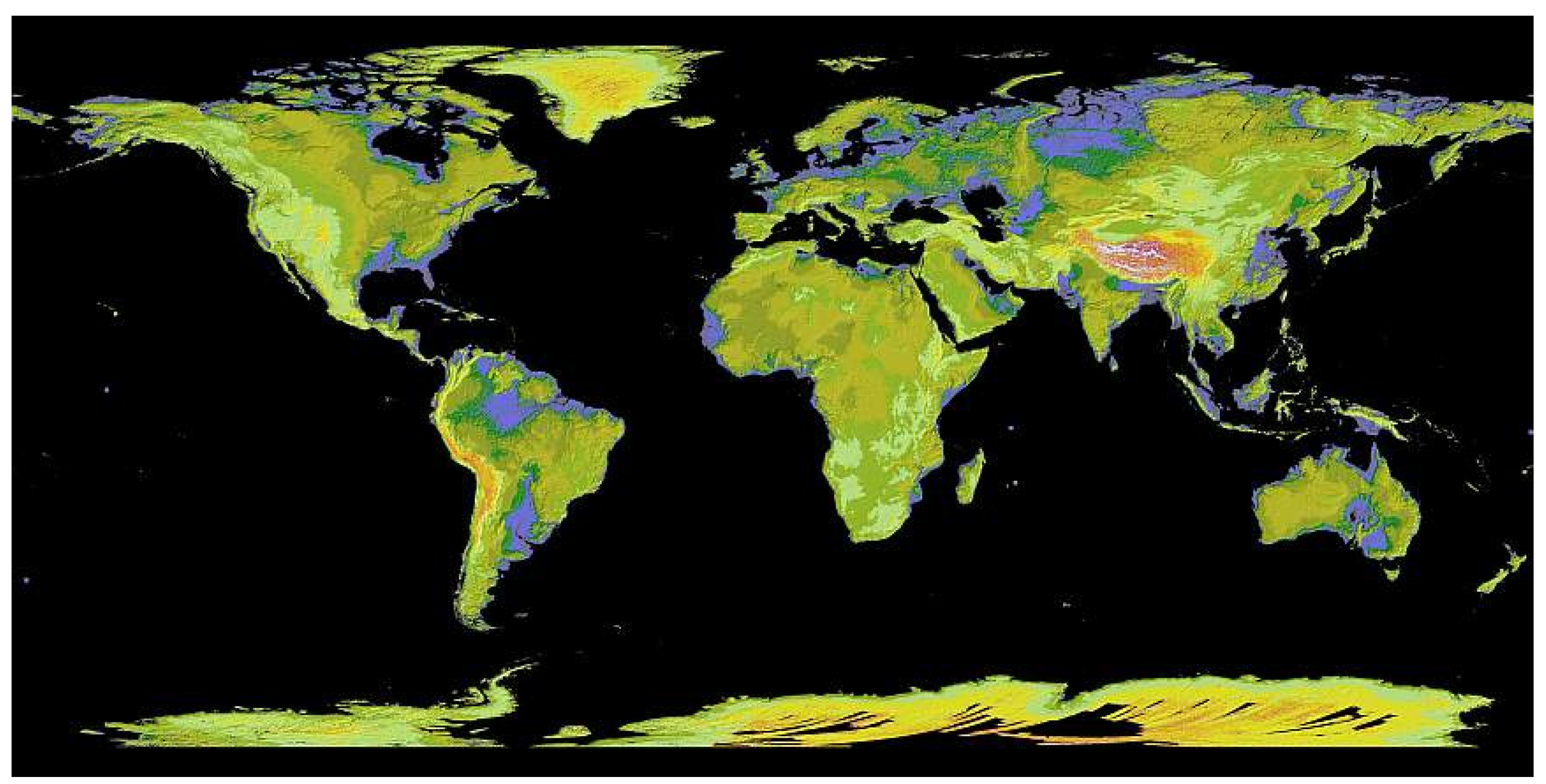
On June 29, 2009, the NASA and METI jointly released the global digital elevation model (GDEM) of the Earth’s land surface (Figure 1), derived from the stereo images acquired by ASTER [2].
The ASTER GDEM is the most up-to-date, complete digital topographic dataset of the Earth available to the public, covering the global land surface from 83 degrees north to 83 degrees south latitude. The GDEM was offered jointly by METI and NASA to the Group on Earth Observations (GEO) at the Summit of Ministers in Cape Town, as a contribution to the Global Earth Observing System of Systems (GEOSS) to serve societal needs.
The ASTER GDEM Version 1 was generated using 1,264,000 Level-1A scenes acquired between March 1, 2000 and November 30, 2007. ASTER GDEM was created by stacking all individual cloud-masked scene DEMs and non-cloud-masked scene DEMs, and then applying various algorithms to remove abnormal data [3,4,5].
The methodology used to produce the ASTER GDEM involved automatic processing of the entire archive:
- Each of the 1,264,118 daytime VNIR scenes that had a stereo pair was stereo correlated to produce individual scene-based DEMs with 30 m postings. This was done using standard photogrammetric methods and a complete camera model of the ASTER VNIR instrument.
- The individual scenes were also passed through a cloud-screening algorithm to identify cloud-contaminated pixels; data from all ASTER bands were used to identify clouds.
- For each output pixel, all of the acceptable DEM values were stacked and averaged, removing residual bad values and outliers. Where only 1 or 2 pixel values were available, the ASTER DEM value was replaced by an available existing reference DEM or was forced to be void if no fill-in DEM was available.
- Certain elevation anomalies, detected by an automated process, were replaced by values from one of several available existing DEMs. For certain other anomalies, where there was no available value to substitute (such as above 83 degrees latitude), a value of −9999 was inserted. For ocean areas, a DEM value of 0 was assigned.
- The mosaicked and averaged DEM values were partitioned into approximately 22,600 1 × 1 degree tiles, posted at 1 arc-second (~30 m at the equator but fewer meters east–west as a cosine function of latitude), projected in rectangular (cylindrical equidistant projection) format, and referenced to the WGS84 ellipsoid. The tile size is 3601 × 3601. The GDEM tiles are signed 16 bit integers in GeoTIFF format. The names of individual data tiles refer to the latitude and longitude at the geometric center of the lower-left corner pixel of the tile. The rows at the north and south edges, as well as the columns at the east and west edges, of each tile overlap and are identical to the edge rows and columns in the adjacent tiles.
In 2011, Version 2 was released. Improvements in the GDEM2 resulted from acquiring 260,000 additional scenes to improve coverage, a smaller correlation kernel (5×5 versus 9×9 for GDEM1) to yield higher spatial resolution, and improved water masking. A negative 5 m overall bias observed in the GDEM1 was removed in the newer version.
In August, 2019, the ASTER Science Team released GDEM3, the final version of the GDEM. In addition to the addition of several hundred thousand additional scenes to improve quality, a rigorous, automatic and manual anomaly correction program was undertaken to create the most accurate GDEM possible.
3.2. Anomaly Correction for GDEM3
3.2.1. Initial Corrections
A cloud masking and a statistical approach were used to select the effective data for stacking. Cloud masking cannot completely remove the clouds. In addition, the statistical approach is not always effective for anomaly removal in cases where a small number of scenes were used. At least three stacked scenes are necessary to apply statistical algorithms.
Existing DEMs were used as reference data to correct and replace anomalies or missing data. Table 1 shows the list of the reference DEMs used for ASTER GDEM V3 data. The anomaly data were filled with the reference data according to the priority for usage shown in Table 1. When using Global Multi-resolution Terrain Elevation Data 2010 (GMTED2010) 7.5 sec reference data, only an anomaly larger than 1 km2 was filled with the reference data. Smaller size anomalies less than 1 km2 were filled with two-dimensional interpolation from the perimeter data.
The reference data shown in Table 1 collectively cover all ASTER GDEM voids. All of these reference data are not anomaly free, but the initial ASTER GDEM V3 was nearly void free except for Greenland and Antarctica.
3.2.2. GDEM Error Mask Generation
The GDEM error mask was created in three major steps. First, the input GDEM, described above, (both Version 2 and Version 3) was compared to Shuttle Radar Topography Mission (SRTM) [5] and PRISM (30 m DEM available from the Japan Aerospace Exploration Agency (JAXA), created from Advanced Land Observing Satellite (ALOS) Panchromatic Remote-sensing Instrument for Stereo Mapping (PRISM) optical data [10]) for reasonable consistency. Second, the input GDEM was evaluated for the likelihood of errors (such as clouds) based upon its own morphology. Third, the composite mask generated from the first and second steps was expanded by filtering to better include all input GDEM error pixels.
The first step followed qualitative logical probabilities. SRTM has no cloud errors, and the cloud avoidance for PRISM appears to be more consistently effective than the cloud avoidance of the input GDEM. However, both SRTM and PRISM have data voids, and so are not always available for comparison with the input GDEM. Further, SRTM can have interferometric unwrapping errors, although the most significant of those were likely detected and were voided prior to comparison to the input GDEM (see above). In short, SRTM is generally considered reliable and PRISM is considered less error prone than the input GDEM, especially where two or fewer ASTER scenes were used to create GDEM. With that in mind, this first step in creating the GDEM error mask adhered to the following logic:
- SRTM and PRISM not void: Input GDEM pixel was rejected if it differed from both SRTM and PRISM by more than 80 m.
- SRTM and PRISM both void: Input GDEM not rejected.
- SRTM void but PRISM not void: Input GDEM was rejected if more than 80 m different from PRISM, unless input GDEM NUM (number) pixel value was 3 or more.
- PRISM void but SRTM not void: Input GDEM was rejected if more than 80 m different from SRTM.
An initial rejection mask was thus created. The 80 m threshold was determined empirically from extensive experience worldwide, maximizing cloud masking while minimizing the loss of obviously real topography such as dendritic erosion patterns. The mask was then expanded to the eight neighboring pixels of any masked pixel in order to more assuredly include problem areas in the mask.
In the second major step, the mask was then additionally expanded to any pixel that differed “too much” from any neighboring pixel (thus having a slope so high as to be more likely an error, such as a cloud edge, than to be natural topography). The threshold for “too much” was defined as greater than 100 m in the north–south or east–west direction at the equator, and it was defined as 141 m (approximately the square root of 2 times 100) in the northwest–southeast and northeast–southwest directions at the equator. Exceeding the threshold in any direction resulted in GDEM pixel masking. The threshold was decreased appropriately as a cosine function of latitude for all orientations (except north–south) because longitude 1 arc-second pixel spacings decrease with latitude. The (by-chance) round number 100 was (again) determined empirically. Lower thresholds lost too much good topography and higher thresholds accepted too many cloud errors.
At this point, a mask had been created based upon two major steps: (1) comparisons of individual pixels to themselves in other datasets, and (2) comparisons of individual GDEM pixels to their immediate GDEM neighbors. Neither of these steps “look” across significant geography which was found to be a problem. Often edges of clouds were masked but not the cloud interiors (which could be much less steep). Thus, a third step, spatial filtering, was needed to “fill in” the mask.
Extensive testing resulted in an effective filtering method, as follows. Any non-masked pixel was added to the mask if masked pixels were found within a 50 pixel radius in at least 12 of 16 “spoke” directions (north, north–northwest, northwest, west–northwest, west, etc.). The concept here is that small areas need to be additionally masked if they are enclosed by masked pixels or if they are almost (at least 12/16) enclosed by masked pixels. Note that this method does not expand the exterior edges of masked regions (i.e., areas clearly exterior to clouds are preserved as unmasked).
A 5 by 5 median filter of the binary mask (masked versus not masked pixels) was needed to avoid some noise from the 16 detector “spokes”. Previously identified “too steep” pixels were then restored to the mask where eliminated by the 5 by 5 median filter. The mask was then complete and found to be extremely effective.
3.2.3. GDEM Void Filling
The masking of errors in GDEM creates voids that need to be filled. Preferably, these voids are filled with an alternative DEM rather than via interpolation. For consistency, the best DEM to fill the latest GDEM is an earlier GDEM. That results in a final GDEM that is maximally from ASTER and thus most inherently an ASTER product with minimum elevation data from other sources. Using GDEM V2 to fill voids is possible because errors in GDEM V3 were not always spatially coincident with errors in GDEM V2. The newer GDEM uses the ASTER scenes used in GDEM V2 plus additional (more recent) scenes. In general, having more scenes results in fewer errors. However, inclusion of additional cloudy scenes occasionally introduced errors that did not occur in the older GDEM.
Thus, GDEM V2 was the first choice as the elevation model for filling voids of the newer GDEM. Since GDEM V2 has errors too, the same error masking procedure (above) was applied. SRTM, where available, was the elevation model of second choice to be used as fill. This was the reprocessed SRTM (e.g., ICESat adjusted original radar swaths) that was concurrently (circa 2012–2018) generated for the NASADEM project. (The original SRTM had been the primary fill for all prior versions of GDEM.) Some interferometric unwrapping errors were removed from the NASADEM SRTM (and generally replaced with GDEM) but no further masking was applied. PRISM ALOS World 3D-30m (AW3D30), where available, was used as third choice, after it was subjected to a masking routine similar to that applied to the GDEM elevation models. Masking PRISM AW3D30 was a precautionary step. Note that after masking GDEM V2, all of the filler elevation models had voids (GDEM V2, SRTM, and PRISM AW3D30), either inherently, or from masking, or both.
The void fill routine is a modified version of the Delta Surface Fill method of Grohman [11]. The published method was modified in order to (1) use filler DEMs with voids, (2) reduce the spread of errors from void edges into the void fill, and (3) improve processing speed. (See Appendix A for further details of the modified procedure.)
With the delta surface calculated and filled, each intermediate DEM (from each filling step) is generated such that (1) the output is the primary DEM where it exists, (2) the output is void where both DEMs are void and (3) the output is the secondary DEM shifted by the filled delta surface where the primary DEM is void and the secondary DEM is not void.
To summarize, the initial GDEM V3, the GDEM V2, and the PRISM DEM were error masked via select comparisons to each other and to SRTM. The masks were then expanded to also remove DEM morphologies more likely to be clouds (and other errors) than real terrain. Specially designed filtering improved the masks. Voids in the masked initial GDEM V3 were then sequentially filled with the masked GDEM V2, SRTM, and the masked PRISM DEM (in that order). Interpolation filled any remaining voids. Results for all quads outside Antarctica and Greenland were visually inspected and found to be satisfactory to excellent, with some exceptions. Results for major ice sheets (Antarctica and Greenland), often with few ASTER scene inputs, often have poor-quality and limited utility.
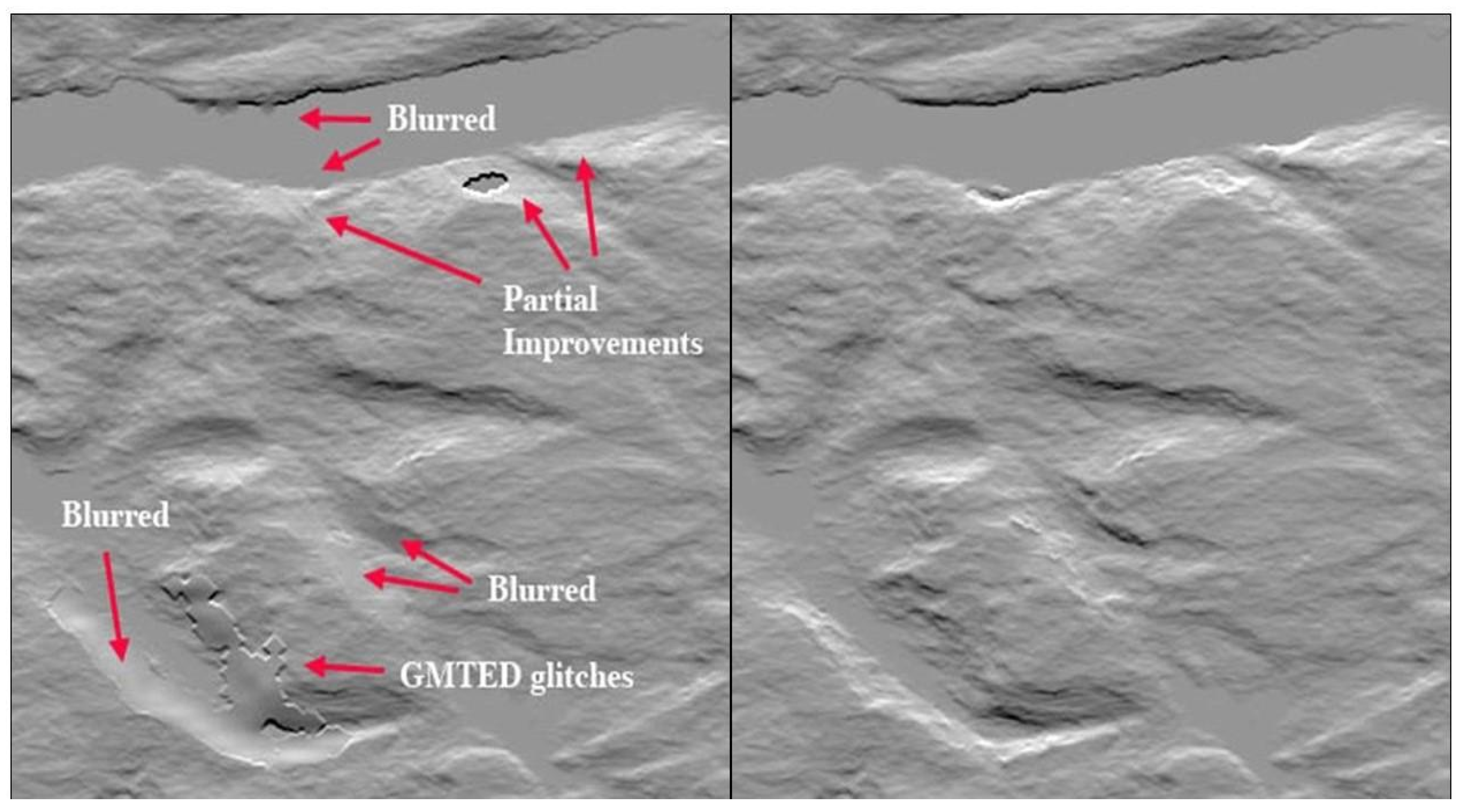
An example of the results of the procedure is shown in Figure 2. A 400 by 400 pixel subarea of tile N60E05 tile was processed using the above process. The input was the GDEM provided by the contractor, who applied some additional void-filling corrections that introduced new artifacts (left image), partially due to the use of poor-quality Global Multi-resolution Terrain Elevation Data 2010 (GMTED 2010) data. The right image shows the final, fully corrected GDEM V3 tile. Note that this area is above 60 degrees north latitude, where there are no SRTM data.
3.3. Data Format and Characteristics
3.3.1. GDEM Characteristics
Each ASTER GDEM tile has two associated files: a DEM file with elevation information and a quality assessment (QA) NUM file. Both files have a dimension of 3601 samples by 3601 lines, which corresponds to 1 degree by 1 degree data area. The names of individual data tiles refer to the latitude and longitude at the geometric center of the lower-left (southwest) corner pixel. For example, the coordinates of the lower-left corner of the tile ASTGTMV003_N00E006 tile are 0 degree north latitude and 6 degrees east longitude. ASTGTMV003_N00E006_dem and ASTGTMV003_N00E006_num files accommodate DEM and QA data, respectively. The rows at the north and south edges as well as the column at the east and west edges of each cell overlap and are identical to the edge row and column in the adjacent cell. The data coverage is north 83 degrees to south 83 degrees. The GDEM collection includes 22,912 tiles. Data product characteristics are summarized in Table 2.
3.3.2. NUM File
A NUM file is provided for each tile to describe the number of images (or swaths) stacked to derive the elevation values from ASTER (GDEM V2 and initial GDEM V3), PRISM, and SRTM. The ASTER scene count is limited here to 50 for both GDEM V2 and GDEM V3 (in some areas the actual scene count exceeds 100). The actual maximum scene count for PRISM is 54 (37 in non-polar areas) and is fully indicated. The actual maximum swath count for SRTM is 23 and is fully indicated. Some other NUM values simply indicate the data type previously used as fill sources in GDEM V2 and the initial GDEM V3 (identified by a single value). See Table 3. The NUM files are presented as single-byte (8 bit, 0-255 Digital Number (DN)) images for easy visual display. The tile size, posting interval, and geometric formats of the NUM files are consistent with the DEM files described in Table 2.
4. Global Water Bodies Database (ASTWBD)
4.1. Background
In addition to ASTER GDEM, the ASTER Global Water Body Database (ASTWBD) was generated as a by-product to correct elevation values of water body surfaces like oceans, rivers, and lakes. The ASTWBD was applied to GDEM such that it has a proper elevation value for a water body surface. The oceans and lakes have a flattened, constant elevation value. Rivers have a stepped-down elevation value from their upper reaches to where they join another river or reach the ocean.
The ASTWBD is the only near-global raster dataset available; it delineates water bodies smaller than 0.2 km2. In addition, the dataset defines the type of water body, and identifies it as ocean, lake or river. Two more, less complete, datasets are publicly available. 1.) The Shuttle Radar Topography Mission (SRTM) Water Body Dataset (SWBD) [12] was created from the SRTM Synthetic Aperture Radar (SAR) mission of 2000 and covers 60 degrees north to 54 degrees south at 30 m resolution and is available from the Land Processes Distributed Active Archive Center (LP DAAC) at https://lpdaac.usgs.gov. It is a binary vector dataset: water or no water. 2.) The Landsat Global Surface Water Explorer [13], developed by the European Commission, is based on 32 years of Landsat data, and maps show change from 80 degrees north to 60 degrees south, at 30 m resolution and is available at https://global-surface-water.appspot.com. The “occurrence” dataset is a binary water/no-water raster dataset, which does not identify the types of water bodies, nor identify shorelines.
4.2. How the ASTWBD Was Created
The ASTWBD was procured from the Sensor Information Laboratory Corporation (SILC) in Tokyo. The SILC used proprietary software to extract water bodies from the ASTER images used to create the GDEM. In addition, considerable hand editing was done on each tile to improve the output from the automatic detection algorithms.
ASTWBD generation consisted of two parts [14]: separation of water bodies from land areas; and classification of detected water bodies into three categories: ocean, river, and lake. The separation process was carried out during scene-based DEM generation using an algorithm that created the GDEM3. For ocean water bodies, the effect of sea ice was manually removed to better delineate ocean shorelines in high-latitude areas. This process was enhanced by reference to Google Earth and GeoCover images. For lake water bodies, the elevation for each lake was calculated from the perimeter elevation data using the mosaic image that covers the entire area of the lake. All lakes with an area greater than 0.2 km2 were identified. Rivers presented a unique challenge, because their elevations gradually step down from upstream to downstream. Initially, visual inspection was required to separate rivers from lakes. A stepwise elevation assignment, with a step of one meter, was carried out by manual or automated methods, depending on the situation.
4.3. The Dataset Container
The ASTWBD zipped tiles accommodate two files: an attribute (*.att) file and an elevation (*.dem) file. Both files have a dimension of 3601 samples by 3601 lines, which corresponds to 1 degree by 1 degree data area at 1 arc-second (~30 m) resolution. The names of individual data tiles refer to the latitude and longitude at the geometric center of the lower-left (southwest) corner pixel. For example, the coordinates of the lower-left corner of the ASTWBDV001_N00E006 tile are 0 degree north latitude and 6 degrees east longitude. ASTWBDV001_N00E006_dem and ASWBDV001_N00E006_att files represent the DEM and attribute layers, respectively. The rows at the north and south edges as well as the column at the east and west edges of each tile overlap and are identical to the edge row and column in the adjacent tile. The data are in geographic latitude/longitude rectangular projection (also called plate carree). The data coverage is north 83 degrees to south 83 degrees. The set of ASTWBD includes 22,912 tiles (Table 4).
4.4. Data Formats and File Name Convention
The attribute file has four values: 0 for land, 1 for ocean, 2 for river, and 3 for lakes, in GeoTIFF format. The accompanying *.dem file has elevation values for all non-land pixels and is also in GeoTIFF format. The data tiles cover 1 by 1 degree areas, and are in rectangular, geographic latitude/longitude projection. Data formats are summarized in Table 5.
The ASTWBD product is a zipped file of the ATT file and corresponding DEM file. An example of the filename is ASTWBDV001_N40W100_XXX.tif, where
ASTWBD = Product short name,
N or S = Northern hemisphere or southern hemisphere,
40 = Latitude of lower left corner,
W or E = Western hemisphere or eastern hemisphere,
100 = Longitude of lower left corner,
XXX = DEM or ATT for data file type, and
Tif = GeoTIFF.
5. Data Availability
The ASTER GDEM and ASTWBD can be searched and downloaded from:
NASA’s Earthdata Search, and
METI’s Japan Space Systems.
Citing ASTER GDEM V3 data:
NASA/METI/AIST/Japan Space Systems, and U.S./Japan ASTER Science Team. ASTER global digital elevation model V003, 2018, distributed by NASA EOSDIS Land Processes DAAC, https://0-doi-org.brum.beds.ac.uk/10.5067/ASTER/ASTGTM.003.
6. Discussion
Creating a global 30 m (or better) DEM, freely available to all users, has been a goal for the Earth science community for decades. Until 2009, the only dataset meeting the resolution criterion was the NGA’s classified DTED, restricted to a few, screened and approved users. In addition, the data could not be published. ASTER’s GDEM Version 1 filled this gaping hole in data characterizing the Earth’s land surface. Further improvements to GDEM1 were incorporated in GDEM2, released in 2011. The final, and most improved, DEM dataset was GDEM3, released in 2019.
There are two more near-global free 30 m DEM datasets available. Data for the SRTM [6] DEM data were acquired in 2000 during an 11 day Shuttle mission. The dataset covers the land surface between 56 degrees north latitude and 60 degrees south latitude. It is not a true global dataset, as it misses northern Europe, northern Asia, Greenland, Iceland, northern Canada, and Antarctica. Numerous studies have validated its accuracy and have found it to be slightly better than ASTER’s accuracy [15]. The data can be downloaded from the USGS EarthExplorer website, in Digital Terrain Elevation Data (DTED) format (designed by the NGA).
The second dataset is Japan’s ALOS World 3D 30 m mesh (AW3D30) [16]. This DEM dataset uses the archived optical data of the Panchromatic Remote-sensing Instrument for Stereo Mapping (PRISM) onboard the Advanced Land Observing Satellite (ALOS, nicknamed “Daichi”). Stereo correlation and processing were completed in March 2016 by Japan Aerospace Exploration Agency (JAXA) collaborating with NTT DATA Corp. and Remote Sensing Technology Center, Japan. The original 5 m DEM was resampled to 1 arc-second (30 m), and released. In April 2019, the most recent update was released. The dataset suffers from many “no-data” areas at high latitudes (above 60 degrees) due to clouds, snow and ice.
Accompanying or stand-alone water masks are available from several sources, as described earlier. Until the 2019 release of the ASTWBD, there was no raster dataset that was global and/or identified the nature of water pixels and provided elevation values for them.
7. Conclusions
We have shown that the first, and still the most complete, 30 m DEM is the ASTER GDEM. Custom software was developed to reduce or eliminate anomalies found in earlier versions, producing an almost artifact-free dataset. Manual inspection of each of the 22,000+ 1 × 1 degree tiles verified that the correction software was effective. While higher-resolution DEMs are available from several commercial vendors, their cost is very high. WorldDEM [17], for example, is a global 12 m resolution dataset, derived from stereo radar pairs from the TanDEM-X satellite mission using radar interferometry. The advertised cost is $6.25/km2. To purchase coverage for the entire land surface of the globe at this per area price would be $900,000,000+ (before quantity discounts). The ASTWBD is a unique raster dataset, depicting the Earth’s water bodies. Accompanying elevation values for every water pixel provide a valuable complementary characteristic.
Author Contributions
Conceptualization, M.A. and H.F.; methodology, R.C. and H.F.; software, H.F. and R.C.; validation, R.C.; writing—original draft preparation, M.A.; writing—review and editing, M.A., R.C., and H.F. All authors have read and agreed to the published version of the manuscript.
Funding
Work by Abrams and Crippen was funded by the National Aeronautics and Space Administration.
Acknowledgments
Work by Abrams and Crippen was performed at the Jet Propulsion Laboratory (JPL), California Institute of Technology, under contract with the National Aeronautics and Space Administration. Refinements of GDEM3 and production of NASADEM, both at JPL, were concurrent and they synergistically improved both elevation models. We gratefully acknowledge support from the NASADEM team (Sean Buckley, Principal Investigator.) Some of the GDEM material in this article was adapted from the GDEM User Guide, written by Abrams and Crippen, and distributed by the LPDAAC with GDEM orders. Some of the ASTWBD material in this article was adapted from the ASTWBD User Guide, written by Abrams, and distributed by the LPDAAC with ASTWBD orders.
Conflicts of Interest
The authors declare no conflict of interest.
Appendix A
In simple terms, the original Delta Surface Fill method is intended to create a void-free DEM from (1) a primary DEM that has voids and (2) a secondary DEM that does not have voids. The secondary DEM fills the voids seamlessly by being adjusted vertically to compensate for height differences (the delta) between the DEMs, with particular focus on the primary DEM’s void edges. Elevations of the secondary DEM within the voids of the primary DEM (where deltas can only be estimated) are adjusted vertically by deltas interpolated from those void edges. Thus, a full delta surface (the DEM difference) is calculated as a simple subtraction where outside the voids, and it is filled by interpolation within the voids. That void-free delta surface is the spatially variable vertical shift that is applied to the filler DEM as it fills the voids of the primary DEM.
For some steps (not the final void-filling step), the delta surface has voids not only from the primary DEM but also from the secondary (filler) DEMs. This often means that some elevations (including void edges) in the primary DEM correspond to voids in the secondary DEM. This is not a severe problem because, unless the DEMs are badly corrupted, all of the delta surface values across a region should be nearly a constant. The delta surface measures general vertical differences between the DEMs (such as reference datum errors, which are spatially constant), various possible warps, and local vertical differences between the DEMs (associated with measurement errors of individual or neighboring pixels, thus having high spatial frequencies and no widespread trends). In short, estimating delta surfaces for voids in the primary DEM is usually performed by interpolation of the delta surface from the edges of those voids. However, if it is performed by interpolation from further away, namely at the edge of the void of the filler DEM, there is usually no large adverse impact. The fill may be somewhat less “seamless” at the edge of the void in the primary DEM, but that “seamlessness” may just have been corruption of the fill to better match errors at the void edge. It may look better (smoother) but be less correct in terms of actual elevations. Thus, applying the Delta Surface Fill method with a filler DEM that has voids does work, but it will (of course) leave remnant voids where both DEMs are void.
The delta surface (as with nearly any difference image) is typically quite noisy. The vast majority of the elevation signal is cancelled and only differences (e.g., errors and possibly temporal differences) in the elevation measurements remain. Systematic errors (reference datums and warps) will remain, and these are what the delta surface is intended to extract and then suppress in the DEM merger. However, random errors also exist pixel by pixel or over small areas. This may be especially true at void edges next to pixels that were voided because they were clearly erroneous or at least unreliable. Interpolation from void-edge pixels can therefore result in a delta surface fill that is particularly noisy. To suppress this, a 5 by 5 pixel median filter was applied to the non-void pixels (only near voids, for speed). Interpolation across the delta surface voids then proceeded using these filtered void-edge pixels.
However, the delta elevations are typically still quite noisy, and so an interpolation method is needed that suppresses local noise and keeps it local. Consequently, a repetitive edge-growing interpolator was used. Pixels in the void directly adjacent to the void edge were interpolated, and then the void pixels next to those were interpolated from the first interpolated pixels. The edge-growing interpolator was run for five iterations. This greatly smoothed the void fill. For speed in global processing, remaining void pixels used direct interpolation and skipped edge growing.
In both the edge-growing interpolator and the interpolator without edge growing, an inverse square root of distance interpolator that looked in 16 directions (north, south, east, west, and approximately west–northwest, northwest, north–northwest, etc.) was applied. Using the inverse square root of distance may be unique. Interpolators often use the inverse square (not square root) of distance to more heavily weight nearby reference points, especially the single nearest reference point. However, to some degree, the opposite approach was desired—to de-emphasize noise in the very nearest reference points. Distant pixels are generally less relevant in most interpolations. However, recall that the delta surface generally measures a fairly uniform value (the elevation signal cancels out). Distant reference pixels are more scattered and therefore less redundantly subject to a single noise source. Giving them extra weighting helps to reduce noise. This is particularly true in the edge-growing interpolator, because typically half of the 16 look directions find pixels that are only a very few pixels away, and close pixels (due to their quantity) are already heavily weighted because of that. The inverse square root of distance formula helps balance the weighting of reference points around the void.
References
- Yamaguchi, Y.; Kahle, A.; Tsu, H.; Kawakami, T.; Pniel, M. Overview of Advanced Spaceborne Thermal Emission and Reflection Radiometer (ASTER). IEEE Trans. Geosci. Remote Sens. 1998, 36, 1062–1071. [Google Scholar] [CrossRef] [Green Version]
- Abrams, M.; Bailey, B.; Tsu, H.; Hato, M. The ASTER Global DEM. J. Am. Soc. Photog. Remote Sens. 2010, 20, 344–348. [Google Scholar]
- Fujisada, H.; Bailey, G.; Kelly, G.; Hara, S.; Abrams, M. ASTER DEM performance. IEEE Trans. Geosci. Remote Sens. 2005, 43, 2707–2714. [Google Scholar] [CrossRef]
- Fujisada HUrai, M.; Iwasaki, A. Advanced methodology for ASTER DEM generation. IEEE Trans. Geosci. Remote Sens. 2011, 48, 5080–5091. [Google Scholar] [CrossRef]
- Fujisada, H.; Urai, M.; Iwasaki, A. Technical methodology for ASTER global DEM. IEEE Trans. Geosci. Remote Sens. 2012, 50, 3725–3736. [Google Scholar] [CrossRef]
- NASA JPL. NASA Shuttle Radar Topography Mission Global 1 Arc Second; NASA EOSDIS Land Processes DAAC: Pasadena, CA, USA, 2013. [CrossRef]
- USGS. USGS Alaska Digital Elevation Models (DEM) 5 Meter; USGS The National Map: Washington, DC, USA, 2013.
- National Resources Canada. Canadian Digital Elevation Data (CDED) 3 Arc Second; Open Government of Canada GeoBase: Ottawa, ON, Canada, 2008.
- USGS. Global Multi-Resolution Terrain Elevation Data 2010 7.5 Arc Second; USGS EarthExplorer: Washington, DC, USA, 2010.
- JAXA. ALOS Global Digital Surface Model 1 Arc Second; JAXA Earth Observation Research Center: Tokyo, Japan, 2017. [Google Scholar]
- Grohman, G.; Kroenung, G.; Strebeck, J. Filling SRTM voids: The Delta Surface Fill method. Photogram. Eng. Remote Sens. 2006, 72, 213–216. [Google Scholar]
- NASA JPL. NASA Shuttle Radar Topography Mission Water Body Data Shapefiles & Raster Files; NASA EOSDIS Land Processes DAAC: Sioux Falls, SD, USA, 2013.
- Pekel, J.; Cottam, A.; Goerlick, N.; Belward, A. High-resolution mapping of global surface water and its long-term changes. Nature 2016. [Google Scholar] [CrossRef] [PubMed]
- Fujisada, H.; Urai, M.; Iwasaki, A. Technical methodology for ASTER Global Water Body Data Base. Remote Sens. 2018, 10, 1860. [Google Scholar] [CrossRef] [Green Version]
- Satge, F.; Bonnet, M.; Timouk, R. Accuracy assessment of SRTM v4 and ASTER GDEM2 over the Altiplano watershed using Icesat/GLAS data. Int. J. Remote Sens. 2015, 45, 465–488. [Google Scholar] [CrossRef]
- Tadono, T.; Nagai, H.; Ishida, H.; Oda, F.; Naito, S.; Minakawa, K.; Iwamoto, H. Initial Validation of the 30 m-mesh Global Digital Surface Model Generated by ALOS PRISM. Int. J. Arch. Photogramm. Remote Sens. Spat. Inf. Sci. 2016, 41, 157–162. [Google Scholar] [CrossRef]
- Apollo Mapping. Available online: https://apollomapping.com/digital-elevation-models/worlddem (accessed on 5 February 2020).
Figure 1.
Colorized, shaded relief depiction of the Advanced Spaceborne Thermal Emission and Reflection Radiometer (ASTER) global digital elevation model Version 1. Ocean is zero elevation, and black. Color scale from (with increasing elevation) purple, blue, green, olive, light green, chartreuse, yellow, orange, dark red, to white. Note the holes in northern Asia, where persistent snow and clouds limited the acquisition of usable scenes.

Figure 2.
Global digital elevation model (GDEM) V3 tile N60E05; 400 by 400 pixel subarea. Left: Input GDEM with errors and artifacts, both original, and introduced in early attempt at correction. Right: Final GDEM tile after corrections.
Figure 2.
Global digital elevation model (GDEM) V3 tile N60E05; 400 by 400 pixel subarea. Left: Input GDEM with errors and artifacts, both original, and introduced in early attempt at correction. Right: Final GDEM tile after corrections.


Table 1.
Reference digital elevation model (DEM) list.
| SRTM1 V3 [6] (First Priority) | Posting: 1 Arc-Second Coverage: North 60 Degrees to South 56 Degrees |
|---|---|
| Alaska DEM [7] (Second priority) | Posting: 2 × 2 arc-seconds Coverage: All Alaska territory |
| CDED* [8] (Canadian Digital Elevation Dataset) (Second priority) | Posting: 3 arc-seconds for latitude 3, 6 and 12 arc-seconds for longitude depending on latitude Coverage: All Canada territory |
| GMTED2010 [9] (Third priority) | Posting: 7.5 arc-seconds Coverage: North 84 degrees to south 56 degrees (except Greenland) |
Table 2.
GDEM characteristics.
| Table | 3601 × 3601 (1 Degree by 1 Degree) |
|---|---|
| Posting interval | 1 arc-second (30 m) |
| Geographic coordinates | Geographic latitude and longitude |
| DEM output format | DEM: GeoTiff, signed 16 bits, and 1m/DN for DEM; NUM: GeoTiff; unsigned 8 bit number of individual scenes used to compile each pixel (maxed at 50); and source of fill for missing ASTER data (see index below) |
| Special DN values | −9999 for void pixels and 0 for sea-level water body |
| Ellipsoid/Geoid | Referenced to the WGS84/EGM96 geoid |
| Coverage | North 83 degrees to south 83 degrees, 22,912 tiles for GDEM |
Table 3.
Contents of NUM file showing number of DEM tiles used, and source of void fill. * 0 = unspecified; ** National Geospatial Intelligence Agency (filled SRTM).
Table 3.
Contents of NUM file showing number of DEM tiles used, and source of void fill. * 0 = unspecified; ** National Geospatial Intelligence Agency (filled SRTM).
| NUM | DEM Source |
|---|---|
| 0–50 | GDEM V3 (0* to 50+ scenes) |
| 60–110 | GDEM V2 (0* to 50+ scenes) |
| 131–184 | PRISM (1 to 54 scenes) |
| 201–223 | SRTM (1 to 23 swaths) |
| 231 | SRTM V3 from initial GDEM V3 |
| 232 | SRTM V2 from initial GDEM V3 |
| 233 | SRTM V2 from GDEM V2 |
| 234 | SRTM with NGA** fill from GDEM V2 |
| 241 | NED from GDEM V2 (USA) |
| 242 | NED from initial GDEM V3 (USA) |
| 243 | CDED from GDEM V2 (Canada) |
| 244 | CDED from initial GDEM V3 (Canada) |
| 245 | Alaska DEM from GDEM V2 |
| 246 | Alaska DEM from initial GDEM V3 |
| 250 | Interpolation |
Table 4.
ASTER Global Water Body Dataset (ASTWBD) and GDEM # tiles.
| #tiles | GDEM3 | ASTWBD | Status | |
|---|---|---|---|---|
| Case 1 | 16,833 | tile | tile | Water present (ocean, lake, river) in tile |
| Case 2 | 6,053 | tile | tile | No water body (=land) in tile |
| (Subtotal) | 22,912 | Number of ASTWBD or GDEM tiles | ||
| Case 3 | 36,874 | no tile | no tile | Ocean in entire tile |
| Total # of tiles | 59,760 | # of tiles in latitude 83 [(83 * 2) * 360 = 59,760] |
Table 5.
ASTWBD formats.
| Tile Size | 3601 × 3601 (1 Degree by 1 Degree) |
|---|---|
| Posting interval | 1 arc-second (~30 m) |
| Geographic coordinates | Geographic latitude and longitude |
| Output format | ATT (attribute) file: GeoTiff, 8 bits; DN values: 1 for ocean, 2 for river, 3 for lake, and 0 for land DEM (elevation) file: GeoTiff, signed 16 bits, 1m/DN, −9999 for land DEM referenced to the WGS84/EGM96 geoid |
| Coverage | North 83 degrees to south 83 degrees, 22,912 tiles for ASTWBD |
© 2020 by the authors. Licensee MDPI, Basel, Switzerland. This article is an open access article distributed under the terms and conditions of the Creative Commons Attribution (CC BY) license (http://creativecommons.org/licenses/by/4.0/).
Share and Cite
MDPI and ACS Style
Abrams, M.; Crippen, R.; Fujisada, H. ASTER Global Digital Elevation Model (GDEM) and ASTER Global Water Body Dataset (ASTWBD). Remote Sens. 2020, 12, 1156. https://0-doi-org.brum.beds.ac.uk/10.3390/rs12071156
AMA Style
Abrams M, Crippen R, Fujisada H. ASTER Global Digital Elevation Model (GDEM) and ASTER Global Water Body Dataset (ASTWBD). Remote Sensing. 2020; 12(7):1156. https://0-doi-org.brum.beds.ac.uk/10.3390/rs12071156
Chicago/Turabian StyleAbrams, Michael, Robert Crippen, and Hiroyuki Fujisada. 2020. "ASTER Global Digital Elevation Model (GDEM) and ASTER Global Water Body Dataset (ASTWBD)" Remote Sensing 12, no. 7: 1156. https://0-doi-org.brum.beds.ac.uk/10.3390/rs12071156
Note that from the first issue of 2016, this journal uses article numbers instead of page numbers. See further details here.