Inferring Surface Flow Velocities in Sediment-Laden Alaskan Rivers from Optical Image Sequences Acquired from a Helicopter


U.S. Geological Survey, Integrated Modeling and Prediction Division, Golden, CO, 80403, USA
*
Author to whom correspondence should be addressed.
Remote Sens. 2020, 12(8), 1282; https://0-doi-org.brum.beds.ac.uk/10.3390/rs12081282
Submission received: 2 March 2020
/
Revised: 13 April 2020
/
Accepted: 15 April 2020
/
Published: 18 April 2020
(This article belongs to the Special Issue Remote Sensing of Flow Velocity, Channel Bathymetry, and River Discharge)
Abstract
:The remote, inaccessible location of many rivers in Alaska creates a compelling need for remote sensing approaches to streamflow monitoring. Motivated by this objective, we evaluated the potential to infer flow velocities from optical image sequences acquired from a helicopter deployed above two large, sediment-laden rivers. Rather than artificial seeding, we used an ensemble correlation particle image velocimetry (PIV) algorithm to track the movement of boil vortices that upwell suspended sediment and produce a visible contrast at the water surface. This study introduced a general, modular workflow for image preparation (stabilization and geo-referencing), preprocessing (filtering and contrast enhancement), analysis (PIV), and postprocessing (scaling PIV output and assessing accuracy via comparison to field measurements). Applying this method to images acquired with a digital mapping camera and an inexpensive video camera highlighted the importance of image enhancement and the need to resample the data to an appropriate, coarser pixel size and a lower frame rate. We also developed a Parameter Optimization for PIV (POP) framework to guide selection of the interrogation area (IA) and frame rate for a particular application. POP results indicated that the performance of the PIV algorithm was highly robust and that relatively large IAs (64–320 pixels) and modest frame rates (0.5–2 Hz) yielded strong agreement () between remotely sensed velocities and field measurements. Similarly, analysis of the sensitivity of PIV accuracy to image sequence duration showed that dwell times as short as 16 s would be sufficient at a frame rate of 1 Hz and could be cut in half if the frame rate were doubled. The results of this investigation indicate that helicopter-based remote sensing of velocities in sediment-laden rivers could contribute to noncontact streamgaging programs and enable reach-scale mapping of flow fields.
1. Introduction
The largest streamflow monitoring network in Alaska is maintained and operated by the U.S. Geological Survey (USGS) and currently consists of 111 continuous monitoring stations. Although these stations are distributed across the state, Alaska’s vast geographic extent encompasses more than 1,200,000 km of rivers and streams; the majority of these waterways remain ungaged. As a result, the streamflow monitoring network in Alaska is sparse relative to that in the contiguous United States. Whereas the average density of streamgages in the lower 48 states is one gage per 1036 km2, in Alaska the mean area per streamgage is over 16 times greater: 16,735 km2 [1]. Moreover, many of the streamgages in Alaska are located in remote, roadless areas that can only be accessed by helicopter. Maintaining these gages and making periodic streamflow measurements thus places field personnel at risk. In an ongoing effort to improve safety, increase efficiency, and ultimately expand the monitoring network, the USGS is developing noncontact methods to estimate streamflow using data collected from a variety of remote platforms [1]. These remote sensing approaches comprise two broad categories: (1) techniques that rely on observations from satellites [2,3,4]; and (2) near-field techniques that include measurements made from bridges [5], small unmanned aircraft systems (sUAS, or drones), helicopters [6], or fixed-wing aircraft. In this study, we focus on remote sensing of surface flow velocities using optical image sequences acquired from a helicopter deployed above two Alaskan rivers. We outline a particle image velocimetry (PIV)-based workflow that could, along with information on channel bathymetry, contribute to a noncontact streamflow measurement strategy. Note that the term large-scale PIV (LSPIV) is often used to describe the application of PIV techniques, which were originally developed for examining small-scale flows under laboratory conditions, to larger natural rivers. Herein, however, we use the shorter term PIV for brevity.
Near-field remote sensing of streamflow in Alaska presents a number of unique challenges that can complicate if not preclude application of methods developed for smaller rivers and streams in more readily accessible locations. For example, although many prior investigations have estimated surface flow velocities by tracking features visible in image sequences acquired from sUAS, most of these studies seeded the flow with tracer particles to enable the use of various motion estimation algorithms including PIV, particle tracking velocimetry (PTV), and optical flow (e.g., [7,8,9,10,11]). However, introducing artificial tracers in a large Alaskan river like the Yukon, which is the third longest river in the United States and the second largest by flow volume [1], is simply not practical.
An alternative means of estimating surface flow velocities that does not require seeding involves using thermal rather than optical image sequences; the feasibility of this approach has been demonstrated using thermal data acquired from bridges [5], fixed-wing aircraft [12], and sUAS [13]. However, the expression of thermal features is highly sensitive to the air-water temperature contrast, implying that this approach might not be consistently effective over the course of a day. In addition, regulatory constraints and logistical considerations might preclude sUAS-based thermal image acquisition at the time when the air-water temperature contrast is most favorable: before dawn. Other, manned platforms are more expensive to operate and also are limited in several other respects. For example, helicopter exhaust can contaminate thermal images and planes cannot safely fly slow enough to provide the long dwell times most conducive to accurate velocity estimation via PIV.
Given the impracticality of seeding the flow to support large-scale PIV of optical images and the various issues associated with thermal PIV, we evaluated the potential to infer surface flow velocities from optical image sequences using a different type of tracer found in great abundance in many Alaskan rivers: sediment. We hypothesized that naturally occurring differences in the texture and color of the water surface, commonly referred to as ripples and boils, provide sufficient contrast for detection by feature tracking algorithms. This approach builds upon the work of Fujita and Komura [14], who observed “boil vortices” in Japanese rivers and used these features as natural tracers for PIV, assuming that their movement represented the surface flow velocity. Subsequently, Fujita and Hino [15] attributed differences in the color of these boil vortices to variations in the concentration of suspended sediment upwelled from within the water column by turbulence. Chickadel et al. [16] captured a similar phenomenon in a tidal estuary via thermal images acquired above a submerged rocky sill.
Although these boil vortices are not ubiquitous in all rivers and streams and might not be expressed at all discharges, when these features are present they could serve as a natural tracer and thus provide a means of inferring spatial patterns of flow velocity. This approach could be especially well suited to large rivers that transport substantial amounts of sediment in suspension or smaller rivers during periods of high runoff when elevated discharges and increased sediment supply lead to higher concentrations of suspended sediment. Glacially fed rivers, in particular, often convey substantial volumes of sediment during melting periods. For example, although only 5% of the drainage area of Alaska’s Tanana River consists of mountainous glaciated terrain, material originating in these glaciated areas accounts for 76–94% of the river’s sediment load [17].
In addition to stream gaging, characterizing surface velocity fields via remote sensing provides information that is useful in a number of other contexts. From a practical perspective, PIV and other similar techniques allow water surface velocities to be estimated in areas that cannot be accessed by wading or from a boat. Moreover, PIV can resolve low velocities along channel margins, in recirculation zones, and in other small-scale features of the flow field that might not be captured adequately by cross section-based field measurements. Obtaining this type of spatially distributed information is important for many applications in river management. For example, the fate and transport of floating contaminants like oil depend not only upon the main current in the river but also turbulence at the water surface and the location and extent of transient storage zones [18]. Remotely sensed surface velocity fields could be used to identify eddies that represent potential capture zones for the contaminants. Similarly, information on surface velocity patterns could complement tracer studies that use a visible dye to examine dispersion processes [19], which have important implications for the dispersal of juvenile stages of endangered fish species such as sturgeon [20]. Velocity estimates would help guide selection of the location and sampling interval of in-situ sondes used to measure tracer dye concentrations. In a biological context, eddies in rivers provide critical habitat by trapping food for fish and providing a refuge from the primary current [21]. Remote sensing of velocity fields can play a key role in characterizing these micro- to mesoscale habitat features as part of a spatially heterogeneous riverscape [22].
Our work builds upon a growing body of literature on remote sensing of surface flow velocities, summarized in the recent study by Strelnikova et al. [11]. Both Koutalakis et al. [23] and Pearce et al. [10] compared algorithms for inferring flow velocities from optical image sequences, including PIV, PTV, space-time image velocimetry (STIV), a Kanade–Lucas Tomasi optical flow technique, and several other variants. In this study, we selected a single algorithm and instead focused on extending the method to a new domain and establishing a framework to facilitate its effective application. More specifically, we used the ensemble correlation version of PIV advocated by Strelnikova et al. [11] and available within the widely used PIVlab software package [24,25,26] to estimate flow velocities in Alaskan rivers from optical image sequences that were acquired from a helicopter and captured the advection of boil vortices upwelling suspended sediment from within the water column. We also emphasized geo-referencing of the image sequence and derived velocity field, which might be overlooked in studies on smaller streams that only require information on image scale, because PIV output must be spatially referenced to enable comparison with field measurements of flow velocity for accuracy assessment and parameter specification. We developed a workflow that explicitly includes image stabilization and geo-referencing steps to ensure that the motion of the features tracked by the PIV algorithm is due to movement of the water and not the imaging platform.
Additional objectives of this investigation were to identify appropriate image preprocessing techniques and to facilitate selection of two key parameters of the PIV algorithm: (1) the size of the interrogation area within which features are tracked from frame to frame; and (2) the rate at which these frames are acquired. Although guidelines have been proposed [10,11,24], rigorous testing of these parameters in the context of larger rivers is lacking. In addition, we addressed the basic question of how long a river must be imaged to provide reliable velocity information by assessing the sensitivity of velocity estimates to the duration of the image sequence. Overall, we aimed to establish a general framework to guide preprocessing, parameter specification, and mission planning. This type of analysis can also help to determine which types of instrumentation might be well-suited to a particular application and provide guidance for operating these sensors. Our goal was to move beyond trial and error by introducing a more systematic strategy for data collection and PIV parameter specification. Whereas a heuristic approach fails to yield any true, general insight as to how or why a particular solution was effective to some degree, the framework introduced herein ultimately could yield a more process-based explanation as to why a particular configuration either performed well or failed to provide useful information on flow velocities.
To summarize, the objectives of this study were to:
- Assess the feasibility of inferring flow velocities in unseeded, sediment-laden rivers via PIV of optical image sequences acquired from a helicopter.
- Evaluate the utility of different sensor configurations (i.e., image pixel sizes and frame rates).
- Establish a general, modular, spatially explicit workflow for performing PIV analysis.
- Introduce a framework to optimize PIV parameter selection by performing an accuracy assessment based on field measurements of flow velocity.
- Assess the sensitivity of PIV-derived velocity estimates to the duration of the image sequence.
2. Materials and Methods
All of the field measurements and remotely sensed data used in this study are available through a data release hosted by the USGS ScienceBase catalog [27]. The data release consists of a parent landing page with child pages for the individual data sets: field measurements of flow velocity from the Salcha and Tanana Rivers in Alaska and the image sequences acquired from each of these sites.
2.1. Study Area
The need for remotely sensed streamflow information is particularly acute in Alaska, which is the largest of the United States in terms of area but remains sparsely gaged [1]. As part of an ongoing effort to develop robust methods for remote sensing of river discharge, this study focused on two rivers near the city of Fairbanks in central Alaska: the Salcha and Tanana (Figure 1). Basic hydraulic characteristics at the time of data collection are presented in Table 1.
The Salcha is a midsized, gravel-bed river that often flows clear but can transport large amounts of sediment in suspension during periods of high flow. Exceptionally high runoff on the Salcha occurred in 2018 and the discharge of 223 m3/s recorded at a gaging station (USGS 15484000 Salcha River near Salchaket, AK, USA) within our study area on 31 August 2018 was in the 95th percentile of mean daily values for this date. Although no turbidity data were available, 23 suspended sediment samples were collected on the Salcha from 1953 to 1975. A power function was fit to these data to relate suspended sediment concentration in mg/L to discharge in m3/s with an of 0.67. Based on this relationship, the suspended sediment concentration on the Salcha River on the date of image acquisition was estimated to be 55 mg/L. We deployed a mobile weather station as the remotely sensed data were being obtained and recorded a mean wind speed of 1.2 m/s from the southwest.
The Tanana is a large, glacier-fed and thus sediment-laden river [17], representative of the many glacial outwash channels that comprise a large fraction of Alaska’s drainage network. Importantly, the presence of abundant suspended material within these streams could enable surface flow velocities to be inferred via PIV under natural conditions, without the need to seed the flow with artificial tracers. The discharge recorded at the USGS gaging station (15515500) on the Tanana at Nenana, AK, USA, was 1722 m3/s during our data collection on 24 July 2019, approximately the median of the mean daily values observed on this date. Turbidity data were not available for the Tanana, but we used 139 samples of suspended sediment concentration collected between 1963 and 2005 to relate suspended sediment concentration to discharge via a power function with an of 0.92. This relation led to an estimated suspended sediment concentration of 2185 mg/L at the time remotely sensed data were collected. The mean wind speed during image acquisition on the Tanana was 1.3 m/s from the southwest.
2.2. Remotely Sensed Data
The remotely sensed data used in this study were acquired from a Robinson R44 helicopter (Figure 2), a platform that is often used in Alaska to transport field crews to gaging stations in remote, inaccessible terrain for periodic streamflow measurements and maintenance operations. The instrumentation deployed from the helicopter has evolved over time and different cameras were used on the Salcha in 2018 and on the Tanana in 2019. Details regarding the sensors used at each site are provided in the following text and in Table 2. The two instruments spanned a range of technological sophistication (and therefore cost) and collecting data with both allowed us to assess whether a relatively affordable, low-tech system might be sufficient for estimating surface flow velocities or whether a higher-tech, more expensive sensor would be required. For both systems, flight planning involved using information on focal length and the physical dimensions of the camera’s detector array to calculate the flying height required to provide a swath width sufficient to see both banks of the river. Including the banks was critical because distinctive terrestrial features were needed to enable stabilization of the image sequences. In addition, we placed ground control targets along the banks of each river to facilitate image geo-referencing. The locations of these targets were established via postprocessed kinematic (PPK) global positioning system (GPS) surveys with a horizontal positional accuracy of approximately 2 cm.
High spatial resolution images of the Salcha were acquired on 31 August 2018 while the helicopter hovered at a predefined waypoint above a reach of the river where the channel widened and the flow diverged before entering a meander bend (Figure 1b). The images were obtained by a Hasselblad A6D-100c digital mapping camera [28] deployed within a pod mounted on the landing gear of the helicopter, as illustrated in Figure 2a. The instrumentation package within the pod is shown in Figure 2b and included an ATLANS GPS/Inertial Motion Unit (IMU) that provided precise, high-frequency position and orientation data during the flight. The accuracies for this sensor were 0.02° for heading, 0.01° for roll and pitch, 0.05 m for horizontal position, and 0.1 m for vertical position. The Hasselblad was programmed to acquire an image every second (i.e., at the camera’s maximum frame rate of 1 Hz) as the helicopter hovered at a mean flying height of 197 m above the river. The helicopter’s vertical position remained stable throughout the hovering image acquisition, with a standard deviation of flying height of 2.5 m and a range of 9.5 m; these fluctuations had a negligible impact on image scale and were accounted for by the geo-referencing software. The image data were stored on a compact flash memory card within the camera.
The Hasselblad Phocus software package was used to import the raw images, which had a compressed, proprietary format, and export them as .tif files. We then used SimActive Correlator3D software (Version 8.3.5) [29] to geo-reference the image sequence. This process involved using the internal orientation parameters of the camera, trajectory information from the GPS/IMU, a light detection and ranging (lidar) digital elevation model (DEM), and surveyed ground control targets to perform aerial triangulation and bundle adjustment, which resulted in a series of orthorectified GeoTif images with a pixel size of 0.018 m that served as input to the PIV workflow described in Section 2.4.
Video of the Tanana River was acquired on 24 July 2019 using a Zenmuse X5 camera [30] housed within an enclosure connected to a Meeker mount that in turn was attached to the nose of the helicopter (Figure 2a,c). The Zenmuse was not integrated with the GPS/IMU within the pod, but the camera was mounted on a three-axis gimbal to enhance stability. The Zenmuse was operated via remote control from within the helicopter, which allowed the operator to trigger the camera once the aircraft was hovering above the desired waypoint and then view the live video feed. The mean flying height during image acquisition on the Tanana was 591 m above the river; the standard deviation and range of the flying height were 3.9 m and 13 m, respectively. The original video files recorded by the Zenmuse had a frame rate of approximately 30 Hz and were saved in a .mov format. We used a custom MATLAB script to parse the video into individual image frames. Relative to the original, full-frame rate video, we retained only every third frame to obtain an image sequence with a maximum frame rate of 10 Hz. The resulting images were not geo-referenced but provided suitable input for the PIV workflow described below.
2.3. Field Data
In coordination with the image acquisition at each site, we collected direct, in situ field measurements of flow velocity to assess the accuracy of PIV-derived velocity estimates and guide PIV algorithm parameterization. A TRDI RiverRay acoustic Doppler current profiler (ADCP) [31] with a Hemisphere A101 differential GPS with a horizontal precision of 0.6 m [32] was deployed from a catamaran towed behind a boat with an outboard motor. ADCP data were collected along channel-spanning cross sections oriented perpendicular to the primary flow direction. One transect was recorded within the footprint of the Salcha River image sequence (Figure 1b) whereas the greater spatial extent of the images from the Tanana River encompassed two ADCP transects (Figure 1c). The ADCP data were not intended for use as a discharge measurement and a single pass across the channel was performed at each transect. The RiverRay was controlled by an operator in the boat using the TRDI WinRiver II software package, which allowed for real-time visualization of the velocity field throughout the water column as the boat traversed the channel. The ADCP data were postprocessed in WinRiver II and exported as text files that were then imported into the USGS Velocity Mapping Toolbox (VMT) [33]. We used VMT to perform spatial averaging with horizontal and vertical grid node spacings of 1 m and 0.4 m, respectively. VMT’s GIS export tool produced text files consisting of easting and northing spatial coordinates (UTM Zone 6N, NAD83) and the east and north components of the depth-averaged velocity vectors at these locations. Following the recent study by Pearce et al. [10], we used this distilled summary of the ADCP data without applying any kind of correction factor (i.e., velocity index [34]) to estimate the corresponding surface flow velocities from the depth-averaged velocity vectors. Assuming a specific velocity index would have been unnecessarily indirect and would have obfuscated the comparison of field-measured and remotely sensed velocities. Quantitative accuracy assessment of PIV output was based on velocity magnitudes.
2.4. Particle Image Velocimetry (PIV) Workflow
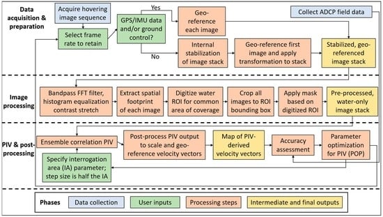
One of the primary objectives of this investigation was to establish a flexible, modular workflow for inferring river surface flow velocities from image sequences. In pursuit of this aim, we developed an approach implemented primarily within MATLAB, making use of the widely used PIVlab add-in as the core PIV algorithm [24,25,26], but also incorporating functionality from the open source FIJI (ImageJ) image processing software package [35]. The various components of the workflow are summarized in Figure 3 and described below.
- The first step toward a map of remotely sensed surface flow velocities is to acquire an image sequence from a helicopter or unmanned aircraft system (UAS) hovering above the river reach of interest, or from any other air- or space-borne platform capable of observing the same area of the river for a duration of at least several seconds. Once the original image sequence has been acquired, the user must select the frame rate to retain for PIV.
- The next step is to stabilize and geo-reference the image sequence, but at this point the workflow diverges depending on whether the images can be geo-referenced based on GPS/IMU data collected onboard the aerial platform and/or ground control targets placed in the field prior to the flight. In this case, a program such as SimActive Correlator 3D [29] can be used to geo-reference and thus stabilize the images. Conversely, if the imaging system is not integrated with a GPS/IMU, the image sequence must first be internally stabilized such that all of the images in the sequence are aligned with one another. We used the TrakEM2 plugin [36] to FIJI for this purpose. The first image in the stabilized sequence is then geo-referenced to an appropriate base image by identifying surveyed ground control targets and/or selecting image-to-image tie points. The resulting set of tie points is used to define an affine transformation from row, column image coordinates to easting, northing spatial coordinates. This transformation is then applied to all frames of the stabilized image stack to place them in the same real world coordinate system.
- The resulting stabilized, geo-referenced image stack is then output to a directory and a FIJI macro called programmatically from within MATLAB to prepare the images for PIV. This image preprocessing involves using FIJI functions to perform FFT bandpass filtering and apply a histogram equalization contrast stretch. The preprocessed images output from FIJI are then imported back into MATLAB.
- Next, the actual spatial footprints of each image in the stack are extracted by automatically tracing the perimeter of the nonzero image pixels. These footprints thus are distinct from the nominal bounding boxes of the images, which might include large areas of no data following stabilization and geo-referencing, particularly if the images are rotated (i.e., oriented at an angle rather than being aligned directly east-west or north-south). To illustrate this step, the footprints extracted from a 1 Hz image sequence from the Tanana River are shown as polygons in Figure 4.
- Overlaying the footprints from all of the images allows the user to identify the area of common coverage throughout the entire stack and digitize a region of interest (ROI) that can also serve as a water-only mask. For the example shown in Figure 4, the ROI for the Tanana River is represented by the blue polygon. This phase of the workflow ensures that only locations encompassed by all of the images are included in the ROI used for PIV.
- To focus the analysis, reduce storage requirements, and improve computational efficiency, all of the images in the stack are cropped to a common bounding box based on the digitized ROI defined in the previous step.
- As a final preprocessing step, the mask corresponding to the digitized ROI is applied to each image to obtain a stack of coregistered water-only images suitable for input to the PIV algorithm that is then exported to a folder.
- The core PIV analysis is performed by calling the ensemble correlation algorithm available within the latest release of PIVlab (version 2.31, published 4 October 2019) programmatically from within MATLAB. Ensemble correlation was developed to facilitate PIV applications in which the seeding density is low and/or the distribution of trackable features is inhomogeneous. In contrast to standard PIV implementations that operate on a frame pair-by-frame pair basis, the ensemble correlation technique averages correlation matrices over the entire image sequence before searching for the correlation peak, which results in more robust velocity estimates, particularly for longer-duration image sequences [11]. The key input to the PIV algorithm that must be specified by the user in units of pixels is the interrogation area (IA) parameter, which sets the area within which features are tracked by computing correlations between successive images. The step size determines the spacing of the velocity vectors output from PIVlab and in this study was always set as half the IA. In our workflow, none of the optional image preprocessing steps available within PIVlab are applied and a single pass of the PIV algorithm is used. Similarly, we did not filter or interpolate the velocity vectors output from PIVlab.
- Once the PIV analysis is complete, the workflow resumes by postprocessing the output from PIVlab, which is in units of pixels/frame. The spatial referencing information for the image stack is used to establish the image scale (i.e., the number of pixels per meter). Along with the known frame rate of the image sequence, this scaling allows the velocity vectors output from PIVlab to be converted to units of meters per second. Similarly, the spatial information associated with the images is used to geo-reference the PIV-derived velocity vectors to the same real world coordinate system as the images. In addition, note that for the newly available ensemble correlation PIV algorithm, time-averaging of the velocity vectors is not necessary. Whereas the older, image pair-based version of PIVlab produced a vector field for each successive pair of images, the ensemble correlation-based implementation generates a single vector field because the underlying correlation analysis is done over the entire image ensemble, not on a frame pair-by-frame pair basis as in the original method.
- The final stage of our workflow involves plotting the PIV-derived velocity vectors as a map overlain on the first image in the stack and assessing the accuracy of the PIV output via comparison with field measurements of flow velocity.
2.5. Accuracy Assessment
Accuracy assessment of PIV-derived velocity estimates was based on the depth-averaged velocity magnitudes recorded in the field by the ADCP. In comparing the PIV- and ADCP-based velocities, we retained only those ADCP measurements that were located within a specified search radius of one of the PIV output vectors. This search radius was set to half the product of the PIV step size parameter, which determined the spacing of the output vector field and was specified as half the IA parameter in units of pixels, and the image pixel size. This definition of the search window ensured that adjacent PIV interrogation areas did not overlap one another and also prevented a given ADCP measurement from being compared to more than one PIV-derived velocity. In cases where the search window included more than one observation from the ADCP, all of the field measurements within the search window were averaged to obtain a single representative value for comparison to the velocity estimated via PIV at the center of the search window.
Once the PIV-derived and ADCP-measured velocities were paired in this manner, we calculated several metrics to quantify the performance of the PIV workflow for various input data sets and parameter values. The root mean squared error (RMSE) served as an index of the precision of the PIV estimates. The absolute accuracy of these estimates was summarized in terms of the mean bias, which we calculated as the difference between the ADCP-measured and PIV-derived velocity magnitudes. A positive value of the mean bias thus indicated underprediction of the ADCP-measured velocity by the PIV algorithm. Conversely, a negative value of the mean bias implied that the velocity inferred via PIV was greater than that measured in the field by the ADCP. In addition to the dimensional RMSE and mean bias in units of m/s, we normalized these values by the mean velocity measured by the ADCP at each site (1.58 m/s for the Salcha River and 1.77 m/s for the Tanana) to express the error metrics in units of percent.
We also performed observed (ADCP) versus predicted (PIV) (OP) regressions [37] and used the OP regression value as a summary of the level of agreement between the PIV-derived velocities and those recorded by the ADCP. Moreover, the slope and intercept of the OP regression provided further information on the performance of the PIV algorithm. Whereas a slope of 1 and an intercept of zero would indicate perfect agreement, any departure from these values implied that the PIV-derived velocities were not scaled correctly (i.e., slope less than or greater than 1) and/or were biased (i.e., nonzero intercept) relative to the ADCP data.
2.6. Evaluating the Effects of Image Preprocessing and Spatial Resolution on PIV-Derived Velocities
We used the hovering image sequence of the Salcha River acquired by the Hasselblad camera to examine how image preprocessing (i.e., step #3 in the PIV workflow outlined in Section 2.4) and pixel size (i.e., ground sampling distance) influenced PIV-derived velocity estimates. To perform this analysis, we resampled the original orthorectified image sequence, which had a pixel size of 1.8 cm, to pixel sizes of 5, 10, and 20 cm. Each of these resampled stacks, as well as the original 1.8 cm-pixel size images, were used in turn as input to the PIV algorithm. We used the stack of images with a 10 cm pixel size as a base case for evaluating the importance of the image preprocessing phase of the PIV workflow. To make this assessment, we performed PIV for both the raw images and images that had been enhanced in FIJI by applying an FFT bandpass filter and a histogram equalization contrast stretch. We compared the PIV output derived from the raw and preprocessed image stacks both graphically, by inspecting maps of the PIV-derived velocity fields, and quantitatively via OP regressions based on field measurements of flow velocity from a transect across the Salcha River.
Our investigation of the effects of image spatial resolution involved performing two separate PIV analyses for each of the four image pixel sizes we considered: 1.8, 5, 10, and 20 cm. For the first type of PIV analysis, we held the IA and step size parameters fixed (in units of pixels) across the four different pixel sizes such that as the pixel size increased so did the spacing of the PIV output vectors, which is determined by the step size parameter. In the second type of PIV analysis, we held the PIV output vector spacing fixed at 6.4 m (i.e., a 64-pixel step size for the image with 10 cm pixels) and adjusted the IA and step size parameters of the PIV algorithm to maintain a consistent vector spacing as the image pixel size varied. For example, for the 5 cm-pixel image, the IA and step size were set to 256 pixels and 128 pixels, respectively, to maintain an output vector spacing of 6.4 m. These two versions of the PIV analysis allowed us to assess whether the effect of a larger image pixel size was a reflection of sparser, less closely spaced PIV output vectors, which would reduce the sample size of the ADCP versus PIV comparison used for accuracy assessment or due to inherent differences in the ability of the PIV algorithm to detect and track features in images with a coarser spatial resolution. We compared the PIV output for different image pixel sizes for both fixed PIV parameters (i.e., variable output vector spacing) and fixed vector output spacing (i.e., variable step size parameter) by producing maps of the PIV-derived velocity fields and computing the various metrics of performance described in Section 2.5.
2.7. Parameter Optimization for PIV (POP)
Successful application of PIV techniques to infer surface flow velocities requires appropriate parameter values, but key inputs to PIV algorithms often are specified iteratively by trial-and-error or on the basis of heuristic guidelines. In this study, we explored an alternative approach, which we refer to as Parameter Optimization for PIV (POP), that involves tuning the PIV algorithm by quantifying the accuracy of velocity estimates derived using various PIV parameter combinations. The high-frame rate video we acquired from the Tanana River allowed us to explore two key dimensions of the PIV parameter space: interrogation area and frame rate. To enable rigorous, quantitative selection of parameter values, we performed PIV for IAs ranging from 16 to 320 pixels in 16-pixel increments and frame rates ranging from 0.5 to 10 Hz. We varied the frame rate by adjusting the number of frames skipped, relative to the 10 Hz maximum frame rate we retained from the original video file, from 1 to 20. For example, skipping 10 frames led to an image sequence sampled at 1 Hz. For each of the 20 IAs and 20 frame rates, we implemented the PIV workflow described in Section 2.4 and computed the RMSE between ADCP-measured and PIV-derived velocities. The combination of IA and frame rate that yielded the smallest RMSE was taken to be the optimal parameter combination. In addition, we used the PIV output for each IA/frame rate combination to compute other metrics of performance including the mean bias, normalized RMSE, normalized mean bias, and OP regression . These results were summarized by producing plots, called POP charts, that display values of each metric as a function of IA and frame rate and thus provide a visual summary of the effects of these parameters on the accuracy of PIV-derived velocities. In essence, the POP framework provided a means of exploiting any available field measurements of velocity to calibrate the PIV algorithm for a particular data set.
2.8. Sensitivity to Image Sequence Duration
An important practical question in remote sensing of flow velocities is how long a river must be imaged in order to derive reliable velocity information. To address this question, we inspected the POP charts produced for the Tanana River to identify IA/frame rate combinations that yielded strong agreement between PIV estimates and field measurements of velocity. We selected an IA of 128 pixels and held this parameter fixed while varying the duration of the image sequence; six different durations were considered. To account for the potentially confounding effect of the number of images, we evaluated image sequences with frame rates of 1 Hz and 2 Hz and truncated the original, full-length sequences for both frame rates to obtain stacks with durations of 2, 4, 8, 16, 32, and 64 s. For example, the 2 s duration image sequence at a frame rate of 1 Hz consisted of a single pair of images whereas the 2 Hz sequence of the same duration included four images. For each of the six durations, the number of images was equal to the duration for the 1 Hz sequence and the number of images in the 2 Hz sequence was twice the duration. Each of these truncated image sequences was used as input to the ensemble correlation PIV algorithm and the resulting velocity estimates were compared to the ADCP field measurements by computing the various accuracy metrics described in Section 2.5.
3. Results
3.1. Image Stabilization and Geo-Referencing
The first steps in our PIV workflow involved stabilizing and geo-referencing the image sequences, but both of these processes were subject to error that introduced some uncertainty into the velocity estimates derived subsequently via PIV. For the hovering image sequence from the Salcha River, data from the GPS/IMU onboard the helicopter and integrated with the Hasselblad camera, along with surveyed ground control targets placed in the field prior to the flight, allowed us to geo-reference each individual image in the stack without an initial, internal stabilization of the stack. The Correlator 3D software we used to orthorectify each image reported an average projection error of 0.39 pixels and an average horizontal error of 1.5 cm, based on three ground control points. This error was less than the size of a single image pixel, the smallest feature displacement between successive frames that the PIV algorithm could possibly detect, and thus was not a significant source of uncertainty in the velocity fields we ultimately derived for the Salcha.
On the Tanana River, the Zenmuse camera used to record video while the helicopter hovered was not integrated with the GPS/IMU and the individual image frames we extracted could not be geo-referenced using the same approach as on the Salcha. Instead, to account for motion of the platform during the video, we used the TrakEM2 FIJI plugin to stabilize the image sequence. One frame from the middle of the stack was used as a reference to which all of the other images were aligned using a scale-invariant feature transform (SIFT) algorithm that detected stable features such as bridges and buildings with fixed spatial locations throughout the entire duration of the video. The maximum alignment error parameter in TrakEM2 was set to five pixels and an affine transformation was used to align the 685 images extracted from the original video. TrakEM2 reported minimum, mean, and maximum displacement errors of 0.626, 0.853, and 1.069 pixels, respectively. For the ground sampling distance of this image sequence, these errors represented distances of 0.094, 0.13, and 0.16 m, respectively. As for the Salcha, these stabilization errors were less than the size of a single image pixel and thus did not introduce any significant uncertainty to the PIV-derived velocity estimates.
Once internally stabilized in this manner, the image stack had to be geo-referenced to enable comparison of PIV-based velocities with field measurements from the ADCP. This phase of the geo-referencing process, performed in the Global Mapper software package (Version 19.0.2) [38] using a satellite image as a base, introduced a greater amount of spatial uncertainty. We used six tie points to establish an affine transformation between the row, column coordinates of one of the stabilized images and easting, northing spatial coordinates. Three of these tie points were ground control targets placed in the field along the south bank of the Tanana and visible in the Zenmuse image. The other three tie points were distinctive, invariant features identified in both the Zenmuse image and the geo-referenced satellite image used as a base. We used the resulting affine transformation matrix to predict the locations of the tie points on the basis of their image coordinates. Comparing these predictions to their actual locations led to a geo-referencing RMSE of 4.33 m. This error was consistent throughout the image sequence because all of the images were stabilized to one another via TrakEM2 and the same affine transformation matrix was applied to each individual frame to geo-reference the entire stack. Within our workflow, this geo-referencing error thus did not influence the PIV-derived velocities, which were based on relative displacements of features between successive images in the stabilized stack.
The absolute geo-referencing error did introduce some uncertainty into the comparison of PIV-derived and ADCP-measured velocities we used to assess accuracy and guide parameter selection. However, the PIV- and ADCP-based velocities were only paired with one another at a spatial resolution set by the spacing of the PIV output vectors (see Section 2.5), which is a function of the PIV step size parameter. In this study, the step size was always set to half the IA and so the potential error associated with image geo-referencing only would have been significant for the smallest IAs we considered. For example, for an IA of 256 pixels, the corresponding step size of 128 pixels represented a spatial distance of 19.2 m and a typical geo-referencing error of 4.33 m thus would have been only 22.5% of the spacing between PIV output vectors, implying that an incorrect pairing of an ADCP measurement with a PIV-derived velocity was highly unlikely.
3.2. Image Preprocessing
To assess the importance of preprocessing images so as to facilitate detection and tracking of features, we performed PIV for both raw and enhanced images of the Salcha River with 10 cm pixels. The results of this analysis are illustrated in Figure 5, which compares the velocity fields generated by PIVlab based on (a) raw and (b) preprocessed images. The primary effect of applying a bandpass filter and contrast stretch was to improve the coherence and consistency of the velocity vectors relative to those derived from the unmanipulated images. Whereas the velocity field in Figure 5a featured large gaps at the bottom of the image and along the left bank farther downstream and low, suspect velocities oriented toward the banks on the right side of the channel, no such gaps were present in Figure 5b and all vectors were directed primarily downstream.
Quantitative accuracy assessment yielded an OP value of 0.96 for both the raw and preprocessed image stacks but the regression for the raw images was based on a smaller sample size () than that for the preprocessed images () due to the gap in the velocity field inferred from the raw images. This gap occurred in the middle of the channel, where the flow field was fairly homogeneous, and so the range of velocities included in the OP regression was similar for both of the image sequences used as input to the PIV algorithm. Had the ADCP transect used for accuracy assessment been located in a different part of the reach that coincided with the spurious vectors derived from the raw image sequence, the OP value for this data set would have been lower.
In any case, these results, as well as our experience with many other raw and preprocessed image stacks, imply that enhancing the original image data leads to improved detection and tracking of features by the PIVlab ensemble correlation algorithm and thus more accurate estimates of flow velocity. Although our workflow involved preprocessing the images in FIJI, many alternative approaches to image preparation are also available. For example, PIVlab includes a contrast-limited adaptive histogram equalization (CLAHE) algorithm and several other image preprocessing options accessible via a graphical user interface. We used FIJI because this package provides a wide range of image processing tools and is freely available, open source, and amenable to scripting, batch processing, and external access (e.g., calling FIJI from within MATLAB). Irrespective of the implementation details, the objective of the preprocessing phase of the PIV workflow is to obtain an enhanced image sequence in which distinct, trackable features can be identified readily by the PIV algorithm.
3.3. Effects of Image Spatial Resolution
Another factor influencing the detectability of advecting surface features is the spatial resolution of the images. To examine this effect, we performed two sets of PIV analyses for image sequences from the Salcha River with pixel sizes of 1.8 (the native resolution of the geo-referenced images), 5, 10, and 20 cm. For the first group of PIV runs, the IA and step size PIV parameters were held fixed while the underlying image pixel size varied, leading to more widely spaced output vectors for images with larger pixels (Figure 6a–d). In the second round of PIV, these parameters were adjusted so as to maintain a constant vector spacing across the different pixel sizes (Figure 6e–h). Table 3 lists the PIV input parameters, output vector spacing, and various performance metrics for each of these iterations.
For the first set of PIV analyses, the images with the highest resolution (1.8 cm pixels) provided a high density of output vectors but also yielded an erratic inferred flow field (Figure 6a) and poor agreement with field measurements of velocity (OP , Table 3). We attributed these poor results to the noise present in the high resolution images and to the small size of the pixels relative to the features advecting at the water surface. Resampling the original, full-resolution image sequence to even a slightly coarser pixel size of 5 cm, however, led to a much more coherent velocity field (Figure 6b) and increased the OP to 0.94. Doubling the resampled pixel size to 10 cm yielded a sparser but still informative representation of the velocity field (Figure 6c) and further increased the OP to 0.96. This configuration led to RMSE and mean bias values of 0.244 and −0.184 m/s, respectively, corresponding to 15.5% and −11.7% of the mean velocity measured in situ by the ADCP. The 10 cm pixel size thus represented a reasonable compromise between image noise, spatial detail, and computational demands and served as a base case for evaluating the effects of image preprocessing described above. Further coarsening the images to 20 cm pixels while holding the PIV input parameters fixed (in units of pixels) led to output velocity vectors that were too widely spaced to provide meaningful insight regarding the flow field within the reach.
For the second round of PIV runs, the IA and step size parameters were adjusted to maintain a constant output vector spacing of 6.4 m, which also ensured that the same set of ADCP measurements were used to assess the accuracy of PIV-derived velocity estimates for the various image pixel sizes we considered. When the vector spacing was held fixed in this manner, distinctions between velocity fields inferred from images with different spatial resolutions were less pronounced (Figure 6e–h). The corresponding OP regression values were also quite similar, ranging from 0.90 for 1.8 cm pixels to 0.96 for 10 cm pixels (Table 3). The images with the smallest pixel size resulted in a slightly more irregular vector field with some voids (Figure 6e), but none of the resampled image sequences led to output that was markedly better or worse than any of the other pixel sizes, given the fixed output vector spacing. Along with the consistency of the accuracy assessment results summarized in Table 3, the similarity of the velocity fields derived from images with pixel sizes varying by an order of magnitude implied that the PIV workflow was robust to the effects of image spatial resolution. As long as the pixel size was 5 cm or greater, the noise present in the original 1.8 cm-pixel images was reduced to a sufficient degree to enable coherent, accurate velocity fields to be inferred via PIV.
Figure 7 illustrates the importance of using an appropriate pixel size (i.e., resampling the original data) and preprocessing images prior to PIV. In essence, PIV algorithms identify distinctive features expressed at the water surface and track their displacement between successive frames to infer flow velocities. We reproduced this process by visually inspecting the first frame in the 10 cm-pixel image sequence and placing a green dot to mark the location of an easily recognizable feature in the preprocessed image shown in Figure 7e, which is a zoomed-in subset of the enhanced image shown in Figure 5b. In this study, this feature represents a boil of upwelling sediment rather than the floating foam, debris, or seeded particles that have been used in most previous applications of PIV (e.g., [11]). The location of the boil in the next frame, recorded by the Hasselblad camera 1 s later, is indicated by the red dot in Figure 7f; the length of this displacement vector is 1.99 m, leading to a plausible velocity estimate of 1.99 m/s. The same start and end points were then overlain on the full resolution (1.8 cm pixel) preprocessed images shown in Figure 7c,d, respectively, as well as the original, raw images in Figure 7a,b. The boil we selected as an example was clearly evident in the coarsened, processed image but was harder to distinguish in the preprocessed image with a smaller pixel size due to the greater noise in this sequence; this feature was not apparent at all in the original, unenhanced images. Spatial resampling and image preprocessing thus were critical steps in the PIV workflow in this case.
3.4. Parameter Optimization for PIV (POP)
In an effort to guide selection of appropriate PIV parameters for a particular application, we used a video from the Tanana River to explore the effects of IA and frame rate on the accuracy of PIV-derived velocity estimates. Our Parameter Optimization for PIV (POP) approach was essentially a form of calibration that involved using velocity measurements collected in the field at the same time as the video to identify the PIV parameters that resulted in the closest agreement between the velocities estimated via PIV and the ADCP reference data. Although the in situ velocity measurements were depth-averaged and the PIV estimates presumably represented approximate surface flow velocities, we did not apply a velocity index to account for the difference between depth-averaged and surface velocities before comparing the PIV estimates to the ADCP measurements, consistent with the recent study by Pearce et al. [10]. In addition, note that a critical consideration in any application of the POP framework is obtaining field data that span a broad range of velocities. In this case, the velocities recorded along two ADCP transects across the Tanana River varied from near 0 to over 2.5 m/s.
Figure 8 summarizes the results of our parameter optimization analysis via matrices with different IAs on the horizontal axis and various frame rates on the vertical axis. The entries in each matrix represent values of the (a) OP regression , (b) normalized RMSE, and (c) normalized mean bias. Figure 8 indicates that for any IA larger than 64 pixels and any frame rate less than 1 Hz, the OP value was greater than 0.89. Similarly, these parameter combinations lead to normalized RMSE values less than 11.7% and normalized bias values less than 4.5% of the reach-averaged mean velocity of 1.77 m/s. These results imply that the ensemble correlation PIV algorithm not only provided highly accurate velocity estimates relative to the ADCP data but also was robust to the specific combination of parameters provided as input.
For the approximately 200 m-wide Tanana River, the features detected via PIV were large enough that even for an IA of 320 pixels, equivalent to 48 m, a sufficient number of trackable features were captured within the IA to enable accurate estimation of flow velocities. Similarly, for the flow velocities on the order of 1.5–2 m/s observed on this river, the displacement of surface features was detectable for frame rates as low as 0.5 Hz (i.e., images acquired every other second). Conversely, PIV performance deteriorated for the smallest IAs and highest frame rates because too few trackable features were present within the 16- or 32-pixel (2.4 or 4.8 m) IAs and/or because those features that were detected did not move far enough between successive images when the frame rate was higher than about 5 Hz.
Although a single particular combination was identified as optimal via the POP approach, Figure 8 indicates that many other IAs and frame rates would have led to accuracies nearly as high. Selecting one of these other pairs of parameters thus could achieve comparable performance while providing more detailed spatial information in the form of more closely spaced PIV output vectors. Figure 9 compares the PIV results from the optimal parameter combination, which leads to a relatively coarse vector spacing due to the large IA, to output based on a smaller IA that yielded an OP of 0.95, a reduction of only 0.04 relative to the optimum and provided a much more detailed representation of the flow field that might be highly desirable, if not essential, for certain applications. In addition, the error metrics summarized in Table 4 indicate that the two parameter combinations yielded similar RMSE and mean bias values. In both cases, the normalized RMSE and mean bias for the Tanana River were smaller in absolute value, but opposite in sign, relative to the RMSE and mean bias observed on the Salcha River. On the Tanana, the PIV-derived velocities tended to slightly underestimate the depth-averaged velocities measured in the field with an ADCP, whereas on the Salcha the PIV estimates were larger than the ADCP measurements.
3.5. Sensitivity to Image Sequence Duration
In addition to our analysis of the effects of the IA and frame rate parameters on the accuracy of PIV-derived velocity estimates, we also used video from the Tanana River to examine the effect of image sequence duration. This sensitivity analysis involved holding the IA fixed at 128 pixels and progressively truncating the original, full-length 1 and 2 Hz image sequences. Repeating the analysis for two different frame rates accounted for the potentially confounding effect of the total number of images as well as the duration of the image sequence. This approach allowed us to address the question of not only how long the helicopter would need to hover to provide reliable velocity information but also whether the number of images, rather than the time period over which they were acquired, was an important factor.
This assessment is summarized in Figure 10 and was based on three metrics that summarized the performance of the PIV algorithm by comparing remotely sensed velocities to field measurements: the OP regression , normalized RMSE, and normalized mean bias. For the image sequence with a frame rate of 1 Hz, very poor agreement between PIV-derived and ADCP-measured velocities was observed for the shortest duration, 2 s sequence, with some improvement for the 4 and 8 s sequences. For dwell times of 16 s or longer, the 1 Hz sequence yielded OP values greater than 0.94, with little improvement for the longer 32 or 64 s durations. The corresponding normalized RMSE and mean bias stabilized around 8% and 0, respectively. These results imply that much shorter image sequences, on the order of 25% of the duration of the Tanana River video we recorded, would have been long enough to provide reliable velocity estimates.
Repeating this sensitivity analysis for an image sequence with a frame rate of 2 Hz enabled us to evaluate whether acquiring the same number of images but over a shorter time period would provide a similar level of agreement between the velocities inferred via PIV and those measured in situ. Figure 10 indicates that even if the dwell time was only 2 s, having as few as four images would yield a moderate OP of 0.67, much higher than the 0.05 for the 2 s, 1 Hz sequence; the normalized RMSE and mean bias also were much less for the 2 Hz sequence. The OP reached 0.93 for a duration of 8 s for the 2 Hz data set, half the time required for the OP to exceed 0.9 for the 1 Hz sequence. These results imply that dwell times as short as 8 s would be adequate if the number of images was increased by collecting data at a higher but still relatively modest frame rate of 2 Hz. The superior performance of the 2 Hz sequence relative to the 1 Hz sequence for a given duration rate provided further evidence of the ability of the ensemble correlation PIV algorithm to provide robust velocity estimates. Strelnikova et al. [11] attributed this capability to the algorithm’s averaging correlation matrices over the image sequence before searching for the correlation peak, which in effect increases the density of features in an image sequence in proportion to the number of images. This characteristic of ensemble correlation PIV makes the technique well-suited to quasistationary flows with a low density of trackable features, as was the case in our study.
4. Discussion
4.1. Remote Sensing of Surface Flow Velocities in Large Rivers
Whereas previous research on remote sensing of surface flow velocities primarily has been directed toward relatively small, slowly flowing streams, this study focused on much larger rivers up to 200 m in width. In addition, rather than seeding the flow with artificial tracers, which can be problematic even in much smaller channels [11] and would be all but impossible on a large river, we inferred flow velocities by exploiting a naturally occurring tracer: boil vortices comprised of upwelling suspended sediment. The advecting boils we tracked using a PIV algorithm might not represent true surface velocities as would be the case for foam, debris, or introduced particles floating on the water surface. Another unique challenge arose in this context: the sediment boil vortices were not rigid features like a discrete floating object but rather a mobile, deforming expression of the flow field itself. These boils represent a surface manifestation, in the form of color differences that create a contrast between the feature and the background water, of turbulent mixing processes within the water column, analogous to the thermal features utilized for PIV in prior studies [5,13]. Although the physics governing sediment boil vortices might be complex and will require further research, the results presented herein demonstrate that these boils are an observable phenomenon [14,15] strongly correlated with depth-averaged velocity magnitudes.
Another innovative aspect of this investigation was that whereas many previous studies have acquired image data from bridge- or bank-mounted cameras or sUAS, we obtained image sequences from a hovering helicopter. This platform allowed us to achieve broader spatial coverage by flying higher than a typical sUAS, which tends to be limited by regulatory constraints and/or endurance (i.e., maximum flight time or battery life). Importantly, the greater extent of the helicopter-based images encompassed both banks of even the larger of the two rivers we examined. This broader field of view thus enabled image stabilization and facilitated not only establishing image scale but also geo-referencing PIV-derived velocity vectors to an established coordinate system. The resulting spatially referenced velocity estimates allowed us to perform a quantitative accuracy assessment based on field measurements of flow velocity acquired with an ADCP.
This accuracy assessment was critical to achieving two of our primary objectives: establishing a general framework for inferring flow velocities via remote sensing and introducing a more rigorous, systematic approach to specifying PIV input parameters. Although Koutalakis et al. [23] and Pearce et al. [10] recently compared different velocity estimation algorithms and Strelnikova et al. [11] examined the influence of the IA and step size parameters on ensemble correlation-based PIV, these studies focused on smaller streams; the extent to which their results might scale up to larger rivers remained untested. Moreover, in practice many applications of PIV tend to proceed on the basis of ad hoc, heuristic guidelines with little rationale for selecting a particular image pixel size, frame rate, or duration. Important factors to consider in making such decisions include the size of the features to be tracked and the rate at which they are advected by the flow. The images must be sufficiently spatially detailed to capture these features and the frame rate must be fast enough to ensure that they do not move so far between successive frames so as to not be trackable but not so fast that their movement from one frame to the next is too small to be detectable. The effects of these sensor characteristics are confounded with those of PIV input parameters, mainly the size of the IA and the number of frames skipped relative to the maximum frame rate of the image sequence. One means of setting these parameters, illustrated in Figure 7, involves visually identifying a feature in an image, measuring its displacement in the next frame, and using this information to select a reasonable IA and step size. Our Parameter Optimization for PIV (POP) framework generalizes and automates this approach by explicitly evaluating a range of IAs and frame rates and identifying that combination which yields the strongest agreement between PIV-derived and field-measured flow velocities. This technique is essentially a form of calibration that can be used to tune a PIV algorithm for application to a specific river of interest, regardless of the size of the channel or the type of features being tracked.
4.2. Implications, Applications, and Limitations
The results of this study have several important implications for operational use of remote sensing techniques for estimating flow velocities; guidelines for data collection based on our experience in Alaska are summarized in Table 5. Our systematic evaluation of various image pixel sizes, PIV IAs, frame rates, and image sequence durations indicated that the native 30 Hz frame rate of the Zenmuse video camera we used was much faster than necessary. The POP analysis summarized in Figure 8 showed that even retaining only every third frame from the original video, thereby reducing the frame rate to 10 Hz, was excessive and that accurate velocity estimates could be derived from image sequences with frame rates as low as 0.5 Hz. However, the sensitivity analysis to image sequence duration presented in Figure 10 indicated that acquiring data at 2 Hz rather than 1 Hz would allow a similar level of accuracy to be achieved in half as much time by doubling the number of images obtained during a given time period. Overall, our results implied that a standard, nonvideo camera capable of triggering from once every other second to twice per second would have been adequate for the large rivers we examined, which had mean flow velocities on the order of 1.5–2 m/s. The reason such modest frame rates would have been acceptable, even for the relatively high flow velocities we observed, was that the images were acquired from a helicopter hovering at a much greater height above the water than previous ground- or sUAS-based studies. When viewed from this elevated perspective, the displacement of features from frame to frame is less for a given frame rate. Had we collected data from a bank-mounted camera or a sUAS deployed 20 m rather than 200 m above the river, the movement of features between frames would have been greater and a higher frame rate might have been necessary. In any case, the POP framework provides a means of evaluating these trade-offs in the context of a particular field site and imaging system.
Similarly, the selection of an appropriate pixel size for mapping velocity fields should be dictated by the application context. For example, a hydrologist might only be concerned with bulk flow characteristics, such as the mean velocity of a channel cross section, for calculating river discharge. For this purpose, a relatively coarse spatial resolution might be adequate. A fisheries biologist or contaminant transport specialist, in contrast, might be interested in eddies and other small-scale features of the flow field and thus would require an image sequence consisting of smaller pixels to obtain more closely spaced PIV output vectors. The ideal spatial resolution also might vary locally within a given reach of river. For the portion of the Salcha River shown in Figure 5 and Figure 6, the ADCP transect used for accuracy assessment was located in an area of flow expansion where widening of the channel produced eddies on both banks that would only be resolved by an image of sufficient resolution. The more homogeneous flow field farther downstream would be more conducive to discharge calculations and could be characterized via coarser-resolution image data. Computational demands are another factor to consider: storage requirements and processing time will scale with pixel size, frame rate, and image sequence duration.
This work was motivated by a particular application: developing noncontact streamflow measurement techniques suitable for large, remote rivers in Alaska. Due to the state’s vast geographic extent, helicopters often are used to transport field personnel to gaging stations for periodic streamflow measurements and maintenance operations. Because helicopters already are deployed to many Alaskan rivers, these platforms could easily be used to acquire hovering image data for PIV to augment or complement conventional, field-based streamgaging. Collecting both field and remotely sensed data simultaneously thus is logistically feasible and would enable POP analyses to be performed for individual streamflow monitoring stations. POP would serve to identify optimal PIV parameters and future monitoring could then be based on remotely sensed data using a site-specific, calibrated PIV algorithm. In addition, water depths recorded by the ADCP (and potentially topographic surveys of the banks and floodplain) would provide the cross-sectional area information needed to calculate discharge; structure from motion photogrammetry could also be used to obtain above-water topography, e.g., [39]. Once the transition is made to noncontact streamflow measurement, the only field activity required would be placing ground control targets for geo-referencing images, but if a GPS/IMU of sufficient accuracy was available, ground control might not be necessary. An efficient strategy might involve a pilot dropping off a hydrographer to make ADCP measurements and place ground control targets and then acquiring hovering image sequences while the field data are being collected; the results summarized in Figure 10 imply that hover durations as short as 8–16 s, depending on frame rate, would be sufficient. Many cameras, including the Zenmuse used in this study, can be controlled by a mobile phone application and thus could be operated easily and safely by the pilot. This approach would not require adding another person to the field crew. The mission could be further simplified and, in principle, performed by a single person if permanent ground control targets can be established at the monitoring station and left in place.
Although remote sensing of flow velocities has clear, demonstrated potential, a number of caveats must also be considered. Most importantly, some kind of visible, trackable features must be present in the river of interest. In this study, we exploited boil vortices in sediment-laden rivers, but this technique will not be applicable to clear-flowing rivers unless some sort of naturally occurring floating material, such as debris, foam, or ice, is available in sufficient abundance to enable PIV or another optical flow algorithm. The timing of image acquisition must be considered during mission planning because at certain sun angles sun glint can degrade image quality and preclude PIV and so can insufficient lighting if flights occur when the sun is too low. In this study, the Salcha River images were acquired around 10:30 local time and the Tanana was imaged beginning at 15:00 local time. Collecting data on overcast, cloudy days would avoid problems due to sun glint. Adverse weather conditions such as rain or snow could degrade image quality and compromise PIV results. Similarly, wind could bias PIV-derived estimates of surface flow velocity by introducing an extraneous, direction-dependent component of motion not driven by the flow of water within the channel. Wind would also make acquisition of stable hovering image sequences more difficult, particularly if lightweight sUAS were used rather than a helicopter. If the water surface is too rough, with rapids or standing waves, PIV might not be effective and this approach is best-suited to lower-gradient rivers with relatively smooth water surfaces. In addition, note that this approach assumes steady flow conditions and is not applicable to rapidly varying flows as might occur during a flash flood or glacial outburst. Site selection for a hybrid field- and remote sensing-based streamflow monitoring station could be directed by the same criteria used to establish conventional streamgages: a straight, uniform channel free of obstructions and backwater effects. The presence of exposed bar surfaces where ground control targets can be easily placed in the field and identified in the images is desirable. Ideally, the flying height and sensor field of view would be sufficient to provide coverage of at least one but preferably both banks to enable image stabilization and geo-referencing.
In addition to these environmental factors, several more practical concerns might constrain the application of remote sensing to velocity mapping. For example, helicopters are more expensive to operate than fixed wing aircraft or sUAS. On board data storage during a flight can be a limiting factor for long deployments, small pixel sizes, high frame rates, and/or long-duration image sequences. The workflow outlined herein involves a number of steps and can be computationally intensive and, for the time being, would most likely have to be implemented in a postprocessing mode, back in the office rather than in real-time in the field. Because the POP framework is essentially an empirical method, calibration of the PIV algorithm ideally would occur on a case-by-case basis for each combination of site and sensor. Moreover, because the foundation of this approach is an assessment of the accuracy of PIV-derived velocity estimates relative to in situ field measurements, having a sufficient sample size that spans a broad range of velocities is critical. In the context of discharge calculations, another important issue is how to convert PIV-derived, presumably surface flow velocities to depth-averaged velocities. Although a velocity index of 0.85 is a common default value for making this conversion, based on an assumed logarithmic velocity profile, this value is by no means universally applicable and ideally would be tuned locally using ADCP data [5,34]. For example, in this study the negative mean bias values on the order of 10%–15% observed on the Salcha (Table 3) indicated that the PIV-derived velocity estimates were larger than the ADCP-based measurements of the depth-averaged velocity, implying that a velocity index of approximately 0.85 might be appropriate for this site. On the Tanana River, however, the mean bias was positive and smaller in absolute value (3.1%, Table 4), indicating that the PIV-derived velocities tended to underestimate the depth-averaged velocity by a small amount and implying a velocity index close to or slightly greater than 1 for this channel.
4.3. Future Research Directions
This initial study points toward several potentially fruitful avenues for additional research. The underlying physics of the sediment boil vortices exploited in this study merit further investigation, building upon the work of Chickadel et al. [16]. Given the encouraging results reported herein, an exciting prospect enabled by this approach is scaling up remote sensing of flow velocities to longer reaches by collecting multiple, overlapping hovers at a series of waypoints along the river. Whereas a basic discharge measurement would only require a single hover, a multistation deployment would yield continuous, detailed, spatially distributed information on velocity patterns. This type of data could help to support contaminant mapping efforts and reach-scale habitat assessments spanning broad geographic extents. In addition, spatially distributed velocity fields, in combination with knowledge of water surface slope, could be used to invert the governing equations of fluid flow to solve for water depth. This approach thus could provide bathymetric data for turbid rivers that are not conducive to passive optical depth retrieval or green lidar.
Other extensions include assessing the potential to perform PIV based on satellite image data, provided sufficiently high spatial resolutions, frame rates, and image sequence durations can be achieved from space. A more practical alternative in the short term might involve collecting data from manned fixed wing aircraft, which would be less expensive and have a greater range than helicopters. The inability to hover could be overcome by using an advanced gimbal system with geo-location and pointing capabilities to obtain longer dwell times. This objective also could be achieved with a motorized mount that could sweep backward as the plane flies forward. Even if only small portions of successive images in a sequence overlap one another, the area of common coverage might be sufficient to extract a cross section. Our results (Figure 10) imply that as long as the same area of the river is captured in approximately 16 images over a duration of 8 s, accurate velocity estimates could be inferred. Thus, while collecting data from manned aircraft might not yield continuous maps, obtaining a series of cross sections could be feasible.
Enabling more widespread application of this approach will require progress in several other areas. Developing flexible, user-friendly software for executing the workflow outlined herein would help to grow a larger community of practitioners. Similarly, working toward a real-time capability in which PIV-derived velocity vectors could be computed and visualized by a sensor operator during flight would facilitate data collection and enable more rigorous quality control while on site. A final research objective is to provide greater process-based insight regarding the applicability and limitations of remote sensing techniques by collecting data from different sizes and types of rivers. The results of these field tests could be used to relate sensor characteristics and PIV parameters to river attributes in a nondimensional framework. The ultimate goal of this effort would be to provide robust, general guidelines so that a POP analysis would not have to be repeated at each new site. Appropriate values of the IA and frame rate could instead be based on the dimensions of the channel and an estimate of the mean flow velocity.
5. Conclusions
Alaska’s vast geographic extent encompasses many large, remote rivers that can be accessed only by helicopter. To augment conventional, field-based streamgaging within the state, which can be expensive, difficult, and potentially dangerous, we evaluated the feasibility of mapping flow velocities in sediment-laden rivers using image sequences acquired from a helicopter. This type of platform can be deployed from a sufficient flying height to include the entire width of the river and provide a view of both banks, which is critical for image stabilization and geo-referencing. Moreover, the ability of a helicopter to hover above the channel facilitates acquisition of image sequences of sufficient duration for reliable velocity estimation. This approach thus can contribute to a noncontact discharge measurement program, which would also require an independent source of information on channel cross-sectional area. In addition, the ability to collect data while hovering at multiple locations along a river opens up the possibility of producing continuous, reach-scale mapping of the flow field. This type of spatially distributed velocity information would capture both bulk flow characteristics and smaller features like eddies to inform studies of dispersion, contaminant transport, and aquatic habitat.
In addition to the larger size of the rivers we considered, another important distinction between this study and most previous research on remote sensing of flow velocities was our use of a natural tracer for PIV rather than artificial, introduced particles. Moreover, instead of assuming the presence of foam or floating debris, we exploited sediment boil vortices that upwell suspended material from within the water column to produce visible, mobile features at the water surface. This approach does not require seeding the flow and thus provides a more practical solution for large, inaccessible rivers. Additional contributions of this study include an evaluation of different sensor configurations, a general workflow for performing PIV analyses, a framework for optimizing PIV input parameters, and an assessment of the sensitivity of PIV output to image sequence duration. The results reported herein support the following conclusions.
- We evaluated the utility of an aerial mapping camera and a relatively inexpensive video camera that had different requirements in terms of ancillary data and supporting software. Although the mapping camera was capable of providing higher spatial resolution (i.e., smaller image pixels), we found that resampling the data to a coarser pixel size was critical for accurate velocity estimation. Similarly, the high frame rate (30 Hz) of the video camera was excessive; reliable velocity fields were inferred from helicopter-based image sequences with frame rates as low as 0.5 Hz in rivers with mean flow velocities on the order of 1.5–2 m/s. These results imply that relatively basic imaging systems could be used to map velocity patterns in large, sediment-laden rivers.
- The general, modular workflow we introduced included an image preparation phase that involved stabilization and geo-referencing, an image processing phase that enhanced the data to facilitate detection and tracking of water surface features such as sediment boil vortices, a PIV analysis phase based on a robust ensemble correlation algorithm, and a postprocessing phase in which the PIV output is scaled, geo-referenced, and compared to field-based velocity measurements for accuracy assessment. Comparison of velocity fields derived from raw and preprocessed images highlighted the importance of image enhancement. This workflow was applied to data acquired from both the digital mapping camera and the video camera and can readily accommodate data from other sensors and platforms.
- Whereas prior applications of PIV have tended to rely on ad hoc, heuristic guidelines, we developed a more systematic, rigorous approach to Parameter Optimization for PIV (POP). The POP framework identifies the combination of two key PIV input parameters, the size of the interrogation area (IA) within which features are tracked and the frame rate at which images are acquired, that yields the strongest agreement between remotely sensed velocities and those measured in the field. Applying this method to video from a 200-m wide river indicated that the ensemble correlation PIV algorithm was robust, with observed versus predicted regression across a broad range of IAs (64–320 pixels) and frame rates (0.5–2 Hz). Poor accuracies occurred only when the pixel size was smaller than the features to be tracked or when the frame rate was too fast to detect the movement of these features between successive images. These results imply that even relatively large IAs and modest frame rates can yield reliable velocity information.
- Analysis of the sensitivity of PIV-derived velocities to image sequence duration indicated that at a frame rate of 1 Hz dwell times as short as 16 s would provide accurate velocity fields, with negligible improvement for longer durations. If the frame rate were doubled to 2 Hz such that the same number of images could be obtained in half as much time, an 8 s duration was sufficient to provide an of 0.93. These results suggest that the number of images, in addition to the time period over which they are acquired, is an important factor and provide further evidence that the ensemble correlation PIV algorithm is highly robust. Although this conclusion was based on a particular sensor and set of input parameters for a specific field site, our results can be used to guide mission planning for subsequent helicopter-based data collection and to inform future efforts to map velocities from fixed wing aircraft and potentially satellite platforms.
- In summary, for the two rivers we considered and the flying heights from which we acquired image data, the spatial resolution of the mapping camera and the frame rate of the video camera we used were excessive. Resampling the data to larger pixels sizes and lower frame rates led to more accurate PIV output. Similarly, sensitivity analysis indicated that the duration of the image sequences we obtained was longer than necessary. All three of these factors—larger pixels, lower frame rates, and shorter durations—would contribute to reduced data storage and computational requirements and favor more widespread application of remote sensing of flow velocities as a viable operational tool.
Author Contributions
Conceptualization, C.J.L. and P.J.K.; methodology, C.J.L. and P.J.K.; software, C.J.L. and P.J.K.; validation, C.J.L. and P.J.K.; formal analysis, C.J.L. and P.J.K.; investigation, C.J.L. and P.J.K.; resources, C.J.L. and P.J.K.; data curation, C.J.L. and P.J.K.; writing–original draft preparation, C.J.L. and P.J.K.; writing–review and editing, C.J.L. and P.J.K.; visualization, C.J.L. and P.J.K.; supervision, C.J.L. and P.J.K.; project administration, C.J.L. and P.J.K.; funding acquisition, C.J.L. and P.J.K. All authors have read and agreed to the published version of the manuscript.
Funding
Funding for this study was provided by the U.S. Geological Survey Water Mission Area.
Acknowledgments
Jon Nelson of the USGS Geomorphology and Sediment Transport Laboratory and several people from the USGS Alaska Science Center contributed to this work, most notably but not limited to Jeff Conaway, Karenth Dworsky, and Heather Best. Adam LeWinter, Peter Gadomski, Dominic Filiano, and Carl Green of the U.S. Army Corps of Engineers Cold Regions Research and Engineering Laboratory assisted helicopter- and field-based data collection; LeWinter designed the Zenmuse camera mount. Jack Eggleston of the USGS Hydrologic Remote Sensing Branch provided logistical and financial support. Any use of trade, firm, or product names is for descriptive purposes only and does not imply endorsement by the U.S. Government.
Conflicts of Interest
The authors declare no conflict of interest.
References
- Conaway, J.; Eggleston, J.; Legleiter, C.; Jones, J.; Kinzel, P.; Fulton, J. Remote sensing of river flow in Alaska—New technology to improve safety and expand coverage of USGS streamgaging. U.S. Geol. Surv. Fact Sheet 2019, 3024. [Google Scholar] [CrossRef] [Green Version]
- Durand, M.; Gleason, C.J.; Garambois, P.A.; Bjerklie, D.; Smith, L.C.; Roux, H.; Rodriguez, E.; Bates, P.D.; Pavelsky, T.M.; Monnier, J.; et al. An intercomparison of remote sensing river discharge estimation algorithms from measurements of river height, width, and slope. Water Resour. Res. 2016, 52, 4527–4549. [Google Scholar] [CrossRef] [Green Version]
- Bjerklie, D.M.; Birkett, C.M.; Jones, J.W.; Carabajal, C.; Rover, J.A.; Fulton, J.W.; Garambois, P.A. Satellite remote sensing estimation of river discharge: Application to the Yukon River, Alaska. J. Hydrol. 2018, 561, 1000–1018. [Google Scholar] [CrossRef] [Green Version]
- Altenau, E.H.; Pavelsky, T.M.; Moller, D.; Pitcher, L.H.; Bates, P.D.; Durand, M.T.; Smith, L.C. Temporal variations in river water surface elevation and slope captured by AirSWOT. Remote Sens. Environ. 2019, 224, 304–316. [Google Scholar] [CrossRef] [Green Version]
- Legleiter, C.J.; Kinzel, P.J.; Nelson, J.M. Remote measurement of river discharge using thermal particle image velocimetry (PIV) and various sources of bathymetric information. J. Hydrol. 2017, 554, 490–506. [Google Scholar] [CrossRef]
- Kinzel, P.; Legleiter, C.; Nelson, J.; Conaway, J.; LeWinter, A.; Gadomski, P.; Filiano, D. Near-field remote sensing of Alaska Rivers. In Proceedings of the Federal Interagency Sedimentation and Hydrologic Modeling Conference (SEDHYD), Reno, NV, USA, 24–28 June 2019. [Google Scholar]
- Tauro, F.; Porfiri, M.; Grimaldi, S. Surface flow measurements from drones. J. Hydrol. 2016, 540, 240–245. [Google Scholar] [CrossRef] [Green Version]
- Detert, M.; Johnson, E.D.; Weitbrecht, V. Proof-of-concept for low-cost and non-contact synoptic airborne river flow measurements. Int. J. Remote Sens. 2017, 38, 2780–2807. [Google Scholar] [CrossRef]
- Tauro, F.; Tosi, F.; Mattoccia, S.; Toth, E.; Piscopia, R.; Grimaldi, S.; Tauro, F.; Tosi, F.; Mattoccia, S.; Toth, E.; et al. Optical Tracking Velocimetry (OTV): Leveraging Optical Flow and Trajectory-Based Filtering for Surface Streamflow Observations. Remote Sens. 2018, 10, 2010. [Google Scholar] [CrossRef] [Green Version]
- Pearce, S.; Ljubičić, R.; Peña-Haro, S.; Perks, M.; Tauro, F.; Pizarro, A.; Dal Sasso, S.; Strelnikova, D.; Grimaldi, S.; Maddock, I.; et al. An Evaluation of Image Velocimetry Techniques under Low Flow Conditions and High Seeding Densities Using Unmanned Aerial Systems. Remote Sens. 2020, 12, 232. [Google Scholar] [CrossRef] [Green Version]
- Strelnikova, D.; Paulus, G.; Käfer, S.; Anders, K.H.; Mayr, P.; Mader, H.; Scherling, U.; Schneeberger, R. Drone-Based Optical Measurements of Heterogeneous Surface Velocity Fields around Fish Passages at Hydropower Dams. Remote Sens. 2020, 12, 384. [Google Scholar] [CrossRef] [Green Version]
- Dugan, J.P.; Anderson, S.P.; Piotrowski, C.C.; Zuckerman, S.B. Airborne Infrared Remote Sensing of Riverine Currents. IEEE Trans. Geosci. Remote Sens. 2014, 52, 3895–3907. [Google Scholar] [CrossRef]
- Kinzel, P.; Legleiter, C. sUAS-Based Remote Sensing of River Discharge Using Thermal Particle Image Velocimetry and Bathymetric Lidar. Remote Sens. 2019, 11, 2317. [Google Scholar] [CrossRef] [Green Version]
- Fujita, I.; Komura, S. Application of Video Image Analysis for Measurements of River-Surface Flows. Proc. Hydraul. Eng. JSCE 1994, 38, 733–738. [Google Scholar] [CrossRef]
- Fujita, I.; Hino, T. Unseeded and Seeded PIV Measurements of River Flows Videotaped from a Helicopter. J. Vis. 2003, 6, 245–252. [Google Scholar] [CrossRef]
- Chickadel, C.C.; Horner-Devine, A.R.; Talke, S.A.; Jessup, A.T.C.L. Vertical boil propagation from a submerged estuarine sill. Geophys. Res. Lett. 2009, 36, L10601. [Google Scholar] [CrossRef] [Green Version]
- Wada, T.; Chikita, K.A.; Kim, Y.; Kudo, I. Glacial Effects on Discharge and Sediment Load in the Subarctic Tanana River Basin, Alaska. Arct. Antarct. Alp. Res. 2011, 43, 632–648. [Google Scholar] [CrossRef] [Green Version]
- Park, I.; Seo, I.W.; Kim, Y.D.; Han, E.J. Turbulent Mixing of Floating Pollutants at the Surface of the River. J. Hydraul. Eng. 2017, 143. [Google Scholar] [CrossRef]
- Nelson, J.; McDonald, R.; Legleiter, C.; Kinzel, P.; Terrell-Ramos, T.; Higashi, Y.; Seo, I.W.; Baek, D.; Lee, D.H.; Ryu, Y. New methods for predicting and measuring dispersion in rivers. E3S Web Conf. 2018, 40, 05052. [Google Scholar] [CrossRef]
- Erwin, S.O.; Bulliner, E.A.; Fischenich, J.C.; Jacobson, R.B.; Braaten, P.J.; DeLonay, A.J. Evaluating flow management as a strategy to recover an endangered sturgeon species in the Upper Missouri River, USA. River Res. Appl. 2018, 34, 1254–1266. [Google Scholar] [CrossRef]
- Angermeier, P.L.; Schlosser, I.J. Species-Area Relationships for Stream Fishes. Ecology 1989, 70, 1450–1462. [Google Scholar] [CrossRef]
- Fausch, K.D.; Torgersen, C.E.; Baxter, C.V.; Li, H.W. Landscapes to riverscapes: Bridging the gap between research and conservation of stream fishes. Bioscience 2002, 52, 483–498. [Google Scholar] [CrossRef] [Green Version]
- Koutalakis, P.; Tzoraki, O.; Zaimes, G. UAVs for Hydrologic Scopes: Application of a Low-Cost UAV to Estimate Surface Water Velocity by Using Three Different Image-Based Methods. Drones 2019, 3, 14. [Google Scholar] [CrossRef] [Green Version]
- Thielicke, W.; Stamhuis, E.J. PIVlab—Towards User-friendly, Affordable and Accurate Digital Particle Image Velocimetry in MATLAB. J. Open Res. Softw. 2014, 2, e30. [Google Scholar] [CrossRef] [Green Version]
- Thielicke, W. The Flapping Flight of Birds—Analysis and Application. Ph.D. Thesis, Rijksuniversiteit Groningen, Groningen, The Netherlands, 2014. [Google Scholar]
- Thielicke, W.; Stamhuis, E.J. PIVlab—Time-Resolved Digital Particle Image Velocimetry Tool for MATLAB. Figshare Dataset 2019, 12. Available online: https://figshare.com/articles/PIVlab_version_1_35/1092508 (accessed on 17 April 2020).
- Legleiter, C.J.; Kinzel, P.J. Field measurements of flow velocity and optical image sequences acquired from the Salcha and Tanana Rivers in Alaska in 2018 and 2019 and used for used for particle image velocimetry (PIV). U.S. Geol. Surv. Data Release 2020. [Google Scholar] [CrossRef]
- HasselbladA6D 100c. Available online: http://static.hasselblad.com/2017/05/A6D-User-Manual-v1.0.3.pdf988 (accessed on 19 February 2020).
- SimActive Correlator3D. Available online: https://www.simactive.com/correlator3d-mapping-software-features.html (accessed on 19 February 2020).
- DJI Zenmuse X5. Available online: https://www.dji.com/zenmuse-x5 (accessed on 19 February 2020).
- TeledyneMarine RiverRayADCP. Available online: http://www.teledynemarine.com/riverray-adcp?ProductLineID=13 (accessed on 19 February 2020).
- HemisphereA101. Available online: https://www.hemispheregnss.com/wp-content/uploads/2019/01/hemispheregnss_a101 (accessed on 20 February 2020).
- Parsons, D.R.; Jackson, P.R.; Czuba, J.A.; Engel, F.L.; Rhoads, B.L.; Oberg, K.A.; Best, J.L.; Mueller, D.S.; Johnson, K.K.; Riley, J.D. Velocity Mapping Toolbox (VMT): A processing and visualization suite for moving-vessel ADCP measurements. Earth Surf. Process. Landf. 2013, 38, 1244–1260. [Google Scholar] [CrossRef]
- Mueller, D.S. extrap: Software to assist the selection of extrapolation methods for moving-boat ADCP streamflow measurements. Comput. Geosci. 2013, 54, 211–218. [Google Scholar] [CrossRef]
- FIJI-ImageJ. Available online: https://imagej.net/Fiji (accessed on 18 February 2020).
- Cardona, A.; Saalfeld, S.; Schindelin, J.; Arganda-Carreras, I.; Preibisch, S.; Longair, M.; Tomancak, P.; Hartenstein, V.; Douglas, R.J. TrakEM2 Software for Neural Circuit Reconstruction. PLoS ONE 2012, 7, e38011. [Google Scholar] [CrossRef] [Green Version]
- Pineiro, G.; Perelman, S.; Guerschman, J.P.; Paruelo, J.M. How to evaluate models: Observed vs. predicted or predicted vs. observed? Ecol. Model. 2008, 216, 316–322. [Google Scholar] [CrossRef]
- GlobalMapperAll-in-one GIS Software. Available online: https://www.bluemarblegeo.com/products/global-mapper.php (accessed on 26 February 2020).
- King, T.V.; Neilson, B.T.; Rasmussen, M.T. Estimating Discharge in Low-Order Rivers With High-Resolution Aerial Imagery. Water Resour. Res. 2018, 54, 863–878. [Google Scholar] [CrossRef] [Green Version]
Figure 1.
(a) Location of the Salcha and Tanana Rivers within the state of Alaska, near the city of Fairbanks. (b) Example image from the Salcha River. (c) Example video frame from the Tanana River. The red arrows in (b,c) represent depth-averaged velocity vectors measured directly in the field with an acoustic Doppler current profiler (ADCP).

Figure 2.
(a) The Robinson R44 helicopter used as a platform to acquire hovering image sequences. (b) Instrumentation housed within the pod mounted on the helicopter’s landing gear. (c) Schematic of the mount used to attach the video camera to the nose of the helicopter. Photo in (a) and schematic in (c) courtesy of Dominic Filiano and Adam LeWinter, respectively, of the U.S. Army Corps of Engineers Cold Regions Research and Engineering Laboratory.

Figure 3.
Flow chart outlining the data, user inputs, processing steps, and outputs of the particle image velocimetry (PIV) workflow.
Figure 3.
Flow chart outlining the data, user inputs, processing steps, and outputs of the particle image velocimetry (PIV) workflow.

Figure 4.
Actual spatial footprints of each image in the 1 Hz image sequence of the Tanana River are represented as rectangular polygons, with the footprint of the displayed image in red with a thicker line. The digitized region of interest (ROI) encompassing the water within the common area of coverage for the entire image sequence is represented by the blue polygon.

Figure 5.
Comparison of PIV-derived velocity vectors derived from (a) raw images and (b) images preprocessed via FIJI. Image pixel size is 10 cm in both cases and the velocity vectors measured in the field with an ADCP are overlain in red for comparison.
Figure 5.
Comparison of PIV-derived velocity vectors derived from (a) raw images and (b) images preprocessed via FIJI. Image pixel size is 10 cm in both cases and the velocity vectors measured in the field with an ADCP are overlain in red for comparison.

Figure 6.
Comparison of PIV-derived velocity fields derived from images with varying pixel sizes for fixed PIV parameters (top row) and fixed output vector spacing (bottom row). Note that the vector length in the top row is dictated by the spacing between vector origins and does not scale with the magnitude of the velocity vectors, which is similar across the four panels.

Figure 7.
Importance of image preprocessing and spatial resolution. Green point represents location of the tracked feature at time 0 and red point indicates the location of the same feature in the next frame in the image sequence, acquired 1 s later. Measured displacement is 1.99 m.
Figure 7.
Importance of image preprocessing and spatial resolution. Green point represents location of the tracked feature at time 0 and red point indicates the location of the same feature in the next frame in the image sequence, acquired 1 s later. Measured displacement is 1.99 m.

Figure 8.
Parameter Optimization for PIV (POP) results for video sequences from the Tanana River. (a) Observed (ADCP) versus predicted (PIV) regression values. (b) Normalized Root Mean Squared Error (RMSE) between field-measured ADCP and PIV-derived velocities. (c) Normalized mean bias between field-measured ADCP and PIV-derived velocities. RMSE and mean bias are normalized by the mean of the ADCP velocity measurements. Note that for display purposes the normalized RMSE and mean bias values in panels (b,c) are expressed as proportions between 0 and 1 and not as percentages between 0 and 100.

Figure 9.
PIV-derived velocity vectors for the (a) optimal parameter combination and (b) an alternative parameter combination that was nearly as accurate but provided a higher density of output vectors. Corresponding observed vs. predicted regression accuracy assessments for the (c) optimal and (d) alternative parameter combinations. Note that the vector length in each panel is dictated by the spacing between vector origins and does not scale with the magnitude of the velocity vectors, which is similar for both panels.

Figure 10.
Sensitivity of the accuracy of PIV-derived velocities to image sequence duration for the Tanana River for a fixed interrogation area of 128 pixels and frame rates of 1 and 2 Hz. OP = Observed (ADCP) vs. Predicted (PIV). The RMSE and mean bias are normalized by the reach-averaged mean velocity recorded by the ADCP: 1.78 m/s.


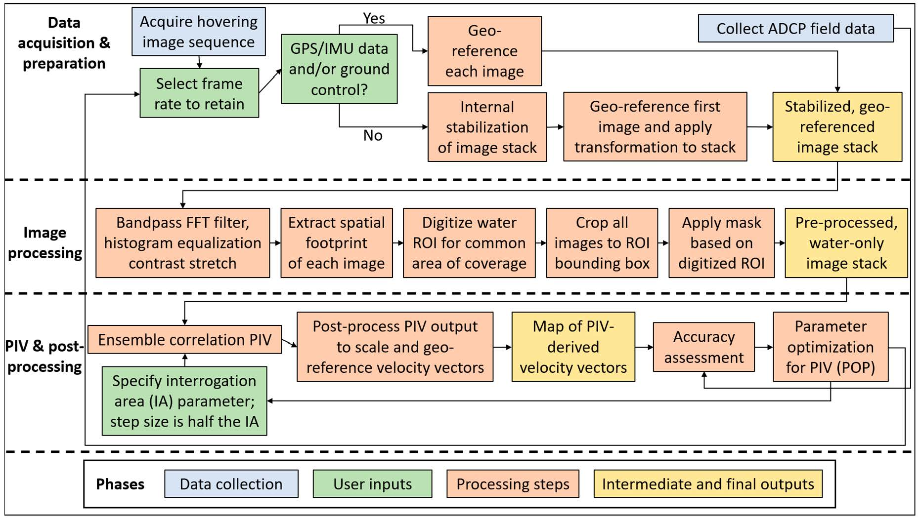
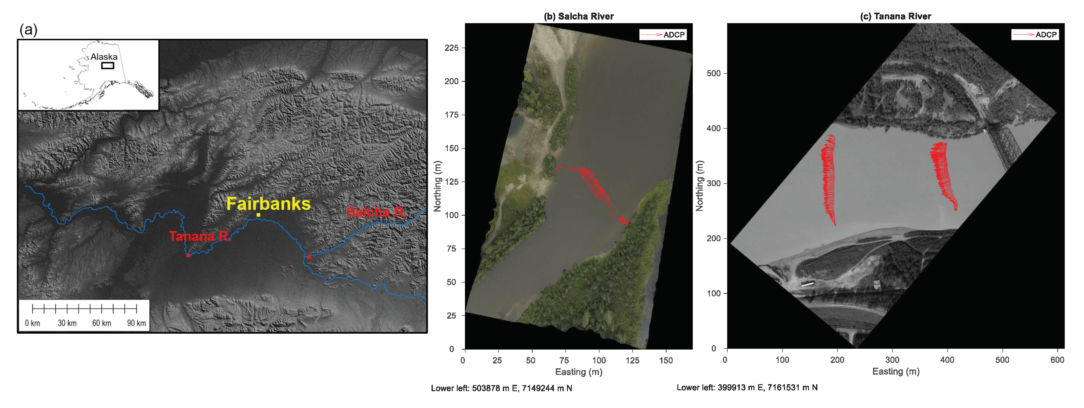
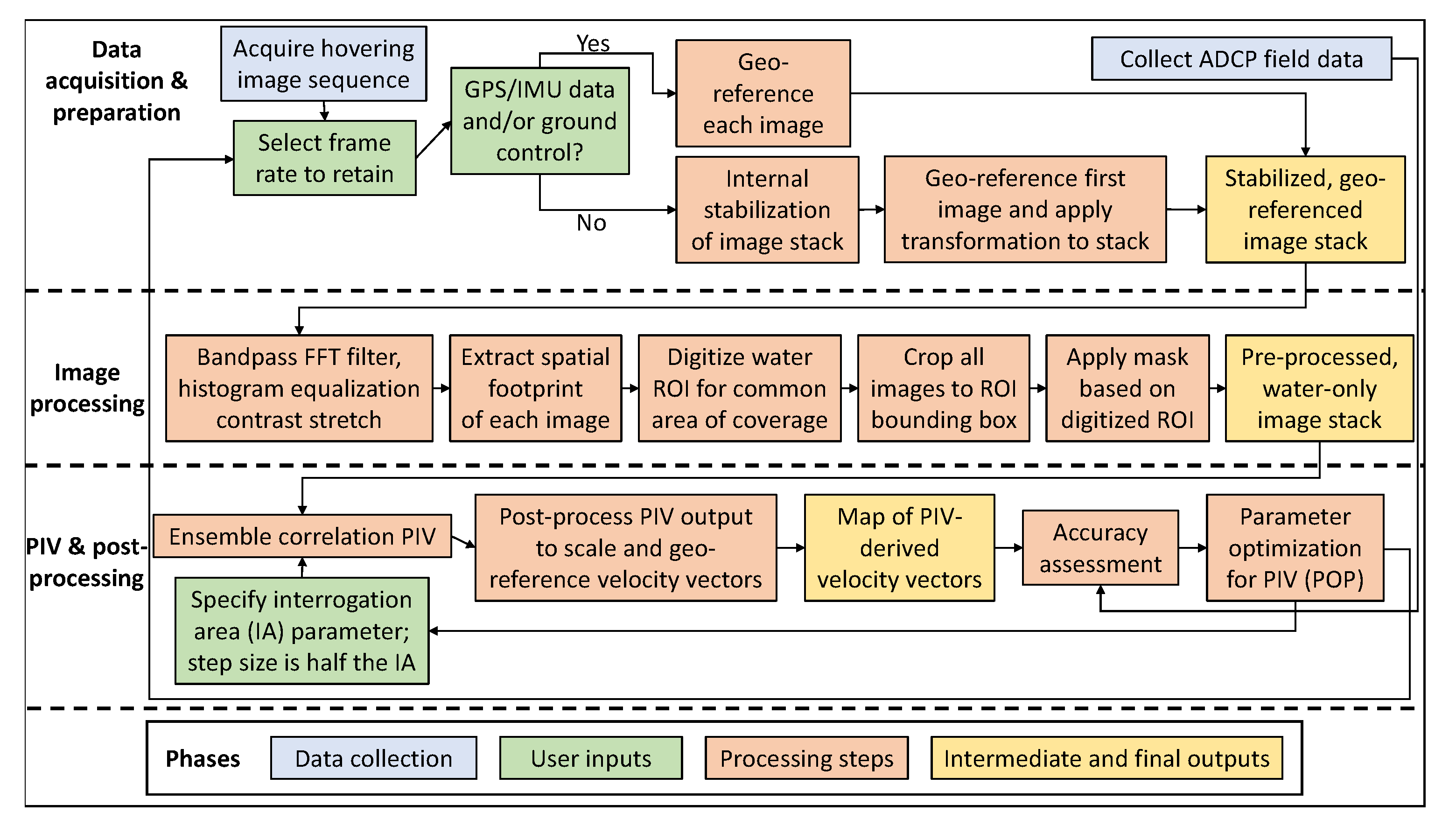
Table 1.
Basic hydraulic characteristics of the Salcha and Tanana Rivers at the time of data collection.
Table 1.
Basic hydraulic characteristics of the Salcha and Tanana Rivers at the time of data collection.
| River | Date of Data Collection | Discharge (m3/s) | Mean Wetted Width (m) | Mean Velocity (m/s) | Mean Depth (m) | Water Surface Slope | Drainage Area (km2) |
|---|---|---|---|---|---|---|---|
| Salcha | 8/31/2018 | 223 | 65 | 1.58 | 2.18 | 0.00046 | 5698 |
| Tanana | 7/24/2019 | 1722 | 190 | 1.77 | 5.12 | 0.00014 | 66,200 |
Table 2.
Characteristics of the sensors used to collect data from the Salcha and Tanana Rivers.
| Camera | Hasselblad A6D-100c | Zenmuse X5 |
|---|---|---|
| Sensor type | CMOS | CMOS |
| Lens (mm) | 50 mm | 15 mm |
| Diagonal field of view (degrees) | 70 | 72 |
| Number of image pixels | 11,600 × 8700 | 3840 × 2160 |
| Pixel size on detector array (m) | 4.6 | 4.5 |
| Frame rate (frames per second) | 1 | 29.97 |
| Image file size (megabytes) | 577 | 1.33 |
| Ground sampling distance/image length/swath width at the 197 m flying height used on the Salcha (m) | 0.0184/160/213 | 0.0592/128/227 |
| Ground sampling distance/image length/swath width at the 591 m flying height used on the Tanana (m) | 0.0543/473/631 | 0.178/383/682 |
| GPS/IMU integration | Yes | No |
| Approximate cost (US dollars) | 20,000 | 2000 |
| Site where deployed | Salcha | Tanana |
| Duration of hover sequence (s) | 68 | 68.5 |
| Number of images at maximum retained frame rate | 68 | 685 |
Table 3.
Summary of PIV results from the Salcha River 2018 data set. OP = Observed versus Predicted; RMSE = root mean squared error; bias is calculated as ADCP–PIV; RMSE and bias are normalized by the mean velocity recorded by the ADCP (1.58 m/s).
Table 3.
Summary of PIV results from the Salcha River 2018 data set. OP = Observed versus Predicted; RMSE = root mean squared error; bias is calculated as ADCP–PIV; RMSE and bias are normalized by the mean velocity recorded by the ADCP (1.58 m/s).
| Pixel Size (m) | Interrogation Area (pixels) | Step Size (pixels) | Vector Spacing (m) | OP | OP Intercept (m/s) | OP Slope | RMSE (m/s) | Mean Bias (m/s) | Normalized RMSE (%) | Normalized Mean Bias (%) |
|---|---|---|---|---|---|---|---|---|---|---|
| 0.018 | 128 | 64 | 1.15 | 0.158 | 0.212 | 0.074 | 1.169 | 0.860 | 74.2 | 54.6 |
| 0.05 | 128 | 64 | 3.2 | 0.941 | 0.157 | 0.952 | 0.224 | −0.098 | 14.2 | −6.2 |
| 0.1 | 128 | 64 | 6.4 | 0.961 | 0.287 | 0.920 | 0.244 | −0.184 | 15.5 | −11.7 |
| 0.2 | 128 | 64 | 12.8 | 0.965 | −0.485 | 1.305 | 0.249 | 0.026 | 15.8 | 1.7 |
| 0.018 | 712 | 356 | 6.4 | 0.903 | 0.389 | 0.918 | 0.336 | −0.263 | 21.3 | −16.7 |
| 0.05 | 256 | 128 | 6.4 | 0.922 | 0.210 | 0.966 | 0.281 | −0.167 | 17.8 | −10.6 |
| 0.1 | 128 | 64 | 6.4 | 0.961 | 0.287 | 0.920 | 0.244 | −0.184 | 15.5 | −11.7 |
| 0.2 | 64 | 32 | 6.4 | 0.924 | 0.323 | 0.912 | 0.266 | −0.193 | 16.9 | −12.3 |
Table 4.
Summary of PIV results from the Tanana River 2019 data set for the two parameter combinations illustrated in Figure 9. Pixel size is fixed at 0.15 m. OP = Observed versus Predicted; RMSE = root mean squared error; bias is calculated as ADCP–PIV; RMSE and bias are normalized by the mean velocity recorded by the ADCP (1.78 m/s).
| Frame Rate (Hz) | Interrogation Area (pixels) | Step Size (pixels) | Vector Spacing (m) | OP | OP Intercept (m/s) | OP Slope | RMSE (m/s) | Mean Bias (m/s) | Normalized RMSE (%) | Normalized Mean Bias (%) |
|---|---|---|---|---|---|---|---|---|---|---|
| 0.556 | 256 | 128 | 19.20 | 0.993 | 0.043 | 0.943 | 0.087 | 0.056 | 4.9 | 3.1 |
| 0.5 | 112 | 56 | 8.4 | 0.950 | 0.209 | 0.858 | 0.155 | 0.057 | 8.7 | 3.2 |
Table 5.
Guidelines for data collection to support PIV on sediment-laden rivers in Alaska.
| Sensor | Standard, nonvideo RGB camera capable of triggering at least once per second |
| Frame rate | 0.5–2 frames per second |
| Flying height | Sufficient to include both banks in the field of view so that image sequence can be stabilized |
| Pixel size | Application-driven, but typically greater than 5 cm; 15 cm sufficient for most cases |
| Hover duration | 8–16 s, depending on frame rate (duration can be shorter for higher frame rates) |
| Acquisition | Trackable features must be present (i.e., flows capable of transporting suspended sediment) Avoid sun glint, but sun cannot be so low as to have insufficient lighting Little or no wind and no rain or snow |
© 2020 by the authors. Licensee MDPI, Basel, Switzerland. This article is an open access article distributed under the terms and conditions of the Creative Commons Attribution (CC BY) license (http://creativecommons.org/licenses/by/4.0/).
Share and Cite
MDPI and ACS Style
Legleiter, C.J.; Kinzel, P.J. Inferring Surface Flow Velocities in Sediment-Laden Alaskan Rivers from Optical Image Sequences Acquired from a Helicopter. Remote Sens. 2020, 12, 1282. https://0-doi-org.brum.beds.ac.uk/10.3390/rs12081282
AMA Style
Legleiter CJ, Kinzel PJ. Inferring Surface Flow Velocities in Sediment-Laden Alaskan Rivers from Optical Image Sequences Acquired from a Helicopter. Remote Sensing. 2020; 12(8):1282. https://0-doi-org.brum.beds.ac.uk/10.3390/rs12081282
Chicago/Turabian StyleLegleiter, Carl J., and Paul J. Kinzel. 2020. "Inferring Surface Flow Velocities in Sediment-Laden Alaskan Rivers from Optical Image Sequences Acquired from a Helicopter" Remote Sensing 12, no. 8: 1282. https://0-doi-org.brum.beds.ac.uk/10.3390/rs12081282
Note that from the first issue of 2016, this journal uses article numbers instead of page numbers. See further details here.